The Number of Minimum $k$-Cuts:
Improving the Karger-Stein Bound

Abstract

Given an edge-weighted graph, how many minimum $k$-cuts can it have? This is a fundamental question in the intersection of algorithms, extremal combinatorics, and graph theory. It is particularly interesting in that the best known bounds are algorithmic: they stem from algorithms that compute the minimum $k$-cut.

In 1994, Karger and Stein obtained a randomized contraction algorithm that finds a minimum $k$-cut in $O(n^{(2-o(1))k})$ time. It can also enumerate all such $k$-cuts in the same running time, establishing a corresponding extremal bound of $O(n^{(2-o(1))k})$. Since then, the algorithmic side of the minimum $k$-cut problem has seen much progress, leading to a deterministic algorithm based on a tree packing result of Thorup, which enumerates all minimum $k$-cuts in the same asymptotic running time, and gives an alternate proof of the $O(n^{(2-o(1))k})$ bound. However, beating the Karger–Stein bound, even for computing a single minimum $k$-cut, has remained out of reach.

In this paper, we give an algorithm to enumerate all minimum $k$-cuts in $O(n^{(1.981+o(1))k})$ time, breaking the algorithmic and extremal barriers for enumerating minimum $k$-cuts. To obtain our result, we combine ideas from both the Karger–Stein and Thorup results, and draw a novel connection between minimum $k$-cut and extremal set theory. In particular, we give and use tighter bounds on the size of set systems with bounded dual VC-dimension, which may be of independent interest.

1 Introduction

We consider the $k\textsc{-Cut}$ problem: given an edge-weighted graph $G=(V,E,w)$ and an integer $k$, delete a minimum-weight set of edges so that $G$ has at least $k$ connected components. This problem is a natural generalization of the global min-cut problem, where the goal is to break the graph into $k=2$ pieces. This problem has been actively studied in theory of both exact and approximation algorithms, where each result brought new insights and tools on graph cuts.

Goldschmidt and Hochbaum gave the first polynomial-time algorithm for fixed $k$, with $O(n^{(1/2-o(1))k^{2}})$ runtime [GH94]. Since then, the exact exponent in terms of $k$ has been actively studied. The textbook minimum cut algorithm of Karger and Stein [KS96], based on random edge contractions, can be adapted to solve $k\textsc{-Cut}$ in $\widetilde{O}(n^{2(k-1)})$ (randomized) time. The deterministic algorithms side has seen a series of improvements since then [KYN07, Tho08, CQX18]. The fastest algorithm for general edge weights is due to Chekuri et al. [CQX18]. It runs in $O(mn^{2k-3})$ time and is based on a deterministic tree packing result of Thorup [Tho08]. Hence, the leading algorithms on the randomized and deterministic fronts utilize completely different approaches, but neither is able to break the $O(n^{(2-o(1))k})$ bound for the problem.

On the lower bounds side, a simple reduction from Max-Weight $(k-1)$-Clique to $k\textsc{-Cut}$ implies that the conjectured time lower bound $\tilde{\Omega}(n^{(1-o(1))k})$ for Max-Weight $(k-1)$-Clique [AWW14] also holds for $k\textsc{-Cut}$. Given the recent interest in fine-grained complexity, for the algorithmic problem of finding the minimum $k$-cut, should the true exponent in $n$ for $k\textsc{-Cut}$ be $k$, $2k$, or somewhere in between?

Another closely related, extremal question concerns the number of minimum $k$-cuts that a graph can have. The algorithms of Karger-Stein, Thorup, and Chekuri et al. can be adapted to enumerate all minimum $k$-cuts in $O(n^{(2-o(1))k})$ time, implying the same bound for the extremal number of minimum $k$-cuts in a graph. To this date, no proof of a better bound—algorithmic or otherwise—is known. On the other hand, there are some graphs (e.g., a cycle with $n$ vertices) where the number of minimum $k$-cuts is $\Omega(n^{k})$. Thus, the mathematical question remains: for the extremal number of minimum $k$-cuts of a graph, should the exponent of $n$ be $k$, $2k$, or somewhere in between?

In recent work [GLL18a], we improved on the algorithmic barrier of $O(n^{(2-o(1))k})$ for the case when the input graph has edge weights that are integers polynomially bounded in $n$. In particular, our deterministic algorithm runs in time $O(k^{O(k)}n^{(2\omega/3+o(1))k})$, where $\omega\leq 2.3738$ denotes the matrix multiplication constant [LG14, Wil12]. Aside from the unfortunate restriction to integer-weighted graphs, our algorithm suffers other disadvantages compared to the previous $k\textsc{-Cut}$ algorithms.

1. When edge weights are integers bounded by $n^{O(1)}$ (in particular, exponent independent of $k$), the reduction from Max-Weight $(k-1)$-Clique no longer holds. Consequently, our algorithm solves an easier variant of $k\textsc{-Cut}$ whose lower bound is only $\Omega(n^{(\omega/3-o(1))k})$ from Unweighted $k$-Clique, and not $\Omega(n^{(1-o(1))k})$.

2. The previous algorithms are “combinatorial”, where ours uses fast matrix-multiplication as a black-box. (See [WW10, ABW15] for discussion about combinatorial and matrix multiplication-based algorithms for $k$-Clique and other problems.) One concrete difference is that our algorithm inherently requires $n^{\Omega(k)}$ space, whereas all of the aforementioned $k\textsc{-Cut}$ algorithms require only $\text{poly}(n)$ space.

3. Our algorithm only finds one minimum $k$-cut and, unlike the previous algorithms, cannot be adapted to find all of them in the same asymptotic running time. (This is a common weakness with algorithms that use matrix multiplication.) Hence, it does not imply any improved bound on the extremal number of minimum $k$-cuts, even for integer-weights.

To summarize, beating either of the $O(n^{(2-o(1))k})$ algorithmic and extremal bounds has remained open for the general case. In this paper, we break these bounds for large enough $k$, and get the first true improvement over the Karger–Stein result for $k\textsc{-Cut}$, in both the algorithmic and extremal settings.

Theorem 1.1 (Enumeration Algorithm).

For any large enough constant $k$, there is a randomized algorithm that enumerates all minimum $k$-cuts in time $O(n^{1.981k})$ w.h.p.

Corollary 1.2 (Extremal Result).

For any large enough constant $k$, there are at most $O(n^{1.981k})$ many minimum $k$-cuts.

1.1 Our Techniques

We believe that an important component of the paper’s contributions are the techniques, which draw on different areas: some of them are perhaps surprising and suggesting directions for further investigation. As mentioned previously, the two leading approaches so far to $k\textsc{-Cut}$—random contractions and tree packing—utilize completely different techniques. Our algorithm is the first to incorporate both approaches, which gives us a broader collection of tools to draw from. In addition, we establish a novel connection to extremal set theory in the context of graph cut algorithms, which may be of independent interest. Finally, our actual $k\textsc{-Cut}$ algorithm resembles the bounded-depth branching algorithms commonly found in fixed-parameter tractable algorithms.

Our $k\textsc{-Cut}$ algorithm is conceptually simple at a high level. Let $S^{*}_{1},\ldots,S^{*}_{k}\subseteq V$ be an arbitrary minimum $k$-cut. We compute a set $\mathcal{A}\subseteq 2^{V}$ of potential subsets of vertices $A\subseteq V$ such that one of these sets is exactly $S^{*}_{i}$ for some $i$. We then branch on each computed set $A\in\mathcal{A}$ by guessing $A$ as one component in the targeted $k$-cut, and then recursively calling $(k-1)\textsc{-Cut}$ on $G\setminus A$. It is clear that this algorithm will return the correct $k$-cut on one of its branches. Naturally, to obtain an efficient algorithm, we want the size of $\mathcal{A}$ to be small to ensure a small branching factor, and furthermore, $\mathcal{A}$ should be computable efficiently.

A Simpler Case.

The actual set $\mathcal{A}$ is complicated to describe, so to strive for the simplest exposition that highlights most of our techniques, let us assume (with much loss of generality) that $\mathcal{A}:=\{A\subseteq V:w(\partial_{G}A)\leq\frac{1.49}{k}OPT\}$. (Here, any constant less than $1.5$ will do.) This set $\mathcal{A}$ works if there exists a component $S^{*}_{i}$ satisfying $w(\partial_{G}S^{*}_{i})\leq\frac{1.49}{k}OPT$. This may not always hold, since $\sum_{i}w(\partial_{G}S^{*}_{i})=2\,OPT$ and hence we can only get a bound of $w(\partial_{G}S^{*}_{i})\leq\frac{2}{k}OPT$ in general—but this is a simple case considered for the purposes of intuition. It remains to bound the size of $\mathcal{A}$, and the time to compute it.

1. The Size of $\mathcal{A}$: We can bound the size of $\mathcal{A}$ by $O(2^{k}n)$ using a well-known result in extremal set theory, discussed below. But assuming this bound, we pay a branching factor of $O(2^{k}n)$ to decrease $k$ by $1$, which is great, because if we can continue this process all the way to $k=0$, then our running time becomes $O(2^{k^{2}}n^{k+O(1)})$. (This bound is much better than the one in Theorem 1.1, but recall that we obtained it with much loss in generality.)

2. Computing $\mathcal{A}$: We run a modified Karger-Stein randomized contraction procedure $\text{poly}(n)$ times, and then take the $O(2^{k}n)$ sets $A$ with smallest boundary $w(\partial_{G}A)$. An argument similar to Karger and Stein’s original analysis shows that our computed set contains $\mathcal{A}$ w.h.p., which is good enough for our purposes.

We now sketch the proof of $|\mathcal{A}|\leq O(2^{k}n)$, highlighting its connection to extremal set theory. It will be useful to view each set $A\in\mathcal{A}$ also as the ($2$-)cut $(A,V\setminus A)$ in the graph $G$.

Figure 1.1: An example with $k=10$; we picked $3$ pairs of crossing cuts (i.e., $6$ cuts) each of weight $\frac{1.49}{k}OPT$. Because each of them gives $3$ new pieces, we get $k=10$ parts. But the cut edge weight totals $\frac{6\times 1.49}{k}OPT<OPT$, a contradiction.

For a contradiction, suppose that $|\mathcal{A}|>O(2^{k}n)$. Since $|\mathcal{A}|>2n$, a simple result in extremal set theory says that there exist two such sets $A_{1},A_{2}\in\mathcal{A}$ that cross. Hence, if we cut out the edges in $\partial_{G}A_{1}\cup\partial_{G}A_{2}$, we obtain a $4$-cut, not a $3$-cut. This means that we obtain $3$ new components for the price of $2\cdot\frac{1.49}{k}OPT=\frac{2.98}{k}OPT$. This amortizes to a cost of $\frac{2.98}{3k}OPT$ per additional component. If we can repeat this process—always finding two such crossing cuts whose removal introduces $3$ additional components—then we eventually obtain roughly $k$ components for roughly $(1-\varepsilon)OPT$, contradicting our choice of $OPT$. (See Figure 1.1.) In §3.2, we prove that this process is possible whenever $|\mathcal{A}|>O(2^{k}n)$, implying the desired extremal bound on $|\mathcal{A}|$.

The General Case:

Let’s try to remove the simplifying assumption we made. What if every component $S^{*}_{i}$ satisfies $w(S^{*}_{i})\geq\frac{1.5}{k}OPT$? We could try to take $\mathcal{A}:=\{A\subseteq V:w(\partial_{G}A)\leq\frac{2}{k}OPT\}$, which would certainly contain some $S^{*}_{i}$. We do take this approach, bounding the size of $\mathcal{A}$ (which is substantially more technical), but in this case, it is possible that $|\mathcal{A}|=\Omega(n^{2})$. Branching would result in an overhead of $\Omega(n^{2})$, leading to an $\Omega(n^{2k-O(1)})$ time algorithm, which is no good. Our solution is to still branch on each set in $\mathcal{A}$, but not start over completely in each recursive step. Rather, we keep track of a global measure of progress that amortizes our branching cost over the $k$ recursive calls. In particular, we maintain a nonnegative potential function such that every time we branch on a large set $\mathcal{A}$ (and thus pay an expensive branching factor), the potential function decreases by a lot. This ensures that we do not branch expensively too often.

Our measure of progress is obtained via the tree packing result of Thorup. For a fixed min $k$-cut $\mathcal{S}^{*}=\{S^{*}_{1},\ldots,S^{*}_{k}\}\subseteq V$, we start from a spanning tree $T$ that crosses $\mathcal{S}^{*}$ (i.e., connects $S^{*}_{i}\neq S^{*}_{j}$) at most $2k-2$ times, and run the previous branching procedure by guessing one component $S^{*}_{i}$ at a time. Our potential function is based on the current value of $k$ and the number of edges of the current tree crossing $\mathcal{S}^{*}$. Whenever we branch on an expensive set $\mathcal{A}$ (say, $|\mathcal{A}|=\Omega(n^{2})$), we ensure $\mathcal{A}$ contains some $S^{*}_{i}$ that cuts many edges in $T$, which decreases the potential function substantially.

Connection to VC-Theory:

Consider the set system $(V,\mathcal{A})$ with universe $V$ and subsets $\mathcal{A}$. The set theory result above (saying that any set system with more than $2n$ sets has a pair of crossing sets) implies that the dual VC dimension of $(V,\mathcal{A})$ is at least $2$ when $|\mathcal{A}|>2|V|$; there exist two sets $A_{1},A_{2}\in\mathcal{A}$ such that in their Venn diagram, all four cells are nonempty. (The dual VC dimension is the standard VC dimension of the dual set system.) In § 3.1 and §5, we prove an analogous result for the dual VC dimension $3$, which has not been studied to the best of our knowledge. We also prove better bounds when we want three sets $\mathcal{A}$ partially shattered (i.e., at least $x$ out of $8$ cells in the Venn diagram are nonempty for some $x<8$). This saves the branching cost and allows the global inductive analysis based on the potential function.

1.2 Other Related Work

The $k\textsc{-Cut}$ problem is NP-hard when $k$ is part of the input [GH94]. Karger and Stein gave a randomized Monte-Carlo algorithm with runtime $O(n^{(2-o(1))k})$, via random edge-contractions [KS96]. On the deterministic front, Thorup improved the $O(n^{4k+o(1)})$-time algorithm of [KYN07] to $\tilde{O}(n^{2k})$-time, based on tree packings [Tho08]. These approaches also can be used to enumerate all minimum $k$-cuts, and hence to show that there are at most $O(n^{2k})$ such cuts. Our work [GLL18a] gave a deterministic algorithm that runs in time roughly $O(k^{O(k)}n^{(2\omega/3)k})$ for bounded integer weights, where $\omega\leq 2.3738$ is the matrix-multiplication constant, but it did not bound the number of minimum $k$-cuts. Finally, better algorithms are known for small values of $k\in[2,6]$ [NI92, HO94, BG97, Kar00, NI00, NKI00, Lev00]. The Karger-Stein algorithm was recently extended to Hypergraph k-Cut [GKP17, CXY18], which also gave a bound on the number of minimum $k$-cuts. For the minimum cut ($k=2$), the number of and the structure of approximate min-cuts also have been studied [HW96, BG08].

Approximation algorithms.

The $k\textsc{-Cut}$ problem has several $2(1-1/k)$-approximations due to [SV95, NR01, RS08]; the more general Steiner $k$-cut problem also has the same approximation ratio [CGN06]. This approximation can be extended to a $(2-h/k)$-approximation in time $n^{O(h)}$ [XCY11]. Chekuri et al. [CQX18] studied the LP relaxation of [NR01] and gave alternate proofs for both approximation and exact algorithms with slightly improved guarantees. A fast $(2+\varepsilon)$-approximation algorithm was also recently given by Quanrud [Qua18]. On the hardness front, Manurangsi [Man17] showed that for any $\varepsilon>0$, it is NP-hard to achieve a $(2-\varepsilon)$-approximation in time $\text{poly}(n,k)$ assuming the Small Set Expansion Hypothesis.

FPT algorithms.

Kawarabayashi and Thorup gave the first $f(OPT)\cdot n^{2}$-time algorithm [KT11] for unweighted graphs. Chitnis et al. [CCH⁺16] used a randomized color-coding idea to give a better runtime, and to extend the algorithm to weighted graphs. Here, the FPT algorithm is parameterized by the cardinality of edges in the optimal $k\textsc{-Cut}$, not by the number of parts $k$. Our past work [GLL18b, GLL18a] gave a $1.81$-approximation for $k\textsc{-Cut}$ in FPT time $f(k)\cdot\text{poly}(n)$; this has since been simplified and improved to a $\frac{5}{3}$-approximation by Kawarabayashi and Lin [KL18].

2 Preliminaries

Notations.

Consider a weighted graph $G=(V,E,w)$. For any vertex set $S$, let $\partial_{G}S$ (or $\partial S$ if $G$ is clear from the context) denote the edges with exactly one endpoint in $S$. For a partition $\mathcal{S}=\{S_{1},\ldots,S_{r}\}$ of $V$, let $E_{G}(\mathcal{S}):=\bigcup_{S_{i}\in\mathcal{S}}\,\partial S_{i}$. For a collection of edges $F\subseteq E$, let $w(F):=\sum_{e\in F}w(e)$ be the sum of weights of edges in $F$. For a set of vertices $S\subseteq V$, we also define $w(S):=w(\partial S)$. In particular, for a $k\textsc{-Cut}$ solution $\{S_{1},\ldots,S_{k}\}$, the value of the solution is $w(E_{G}(S_{1},\ldots,S_{k}))$. Let $\kappa(G)$ be number of connected components of $G$.

Thorup’s Tree packing.

The algorithm starts from the following result of Thorup [Tho08].

Theorem 2.1 (Thorup’s Tree Packing).

Given a graph $G=(V,E,w)$ with $n$ vertices and $m$ edges, we can compute a collection $\mathcal{T}$ of $\tilde{O}(k^{3}m)$ trees in time $\tilde{O}(k^{3}m^{2})$ such that for every minimum $k$-cut $\mathcal{S}^{*}=\{S^{*}_{1},\dots,S^{*}_{k}\}$, $\mathbb{E}_{T\in\mathcal{T}}[|E_{T}(S^{*}_{1},\ldots,S^{*}_{k})|]\leq 2k-2$, where the expectation is taken over a uniform random tree $T\in\mathcal{T}$. In particular, there exists a tree $T\in\mathcal{T}$ with $|E_{T}(S^{*}_{1},\ldots,S^{*}_{k})|\leq 2k-2$.

Given a fixed minimum $k$-cut $\mathcal{S}^{*}=\{S^{*}_{1},\dots,S^{*}_{k}\}$, we say a tree $T$ is a T-tree if it crosses $\mathcal{S}^{*}$ at most $2k-2$ times. If we choose a T-tree $T\in\mathcal{T}$, we get the following problem: cut some $\leq 2k-2$ edges of $T$ and then merge the connected components into exactly $k$ components $S_{1},\ldots,S_{k}$ so that $E_{G}(S_{1},\ldots,S_{k})$ is minimized. Thorup’s algorithm accomplishes this task using brute force: try all possible $O(n^{2k-2})$ ways to cut and merge, and output the best one. This gives a runtime of $\widetilde{O}(n^{2k-2}m)$ [Tho08]. The natural question is: can we do better than brute-force?

Enumerating Small Cuts via Karger-Stein.

Our algorithm also uses a subroutine inspired by the Karger-Stein algorithm, which can generate all $\alpha$-minimum cuts in a graph, (i.e., those with cut value at most $\alpha$ times the min-cut in the graph) in time $\tilde{O}(n^{2\alpha})$. We note that a slight modification of this algorithm can generate all cuts of size at most $\alpha\cdot\frac{OPT_{H}}{h}$, where $OPT_{H}$ is the minimum $h$-cut value, in essentially the same run-time. The following lemma is proved in §A.1.

Lemma 2.2.

Let $OPT_{H}$ be the weight of the optimum minimum $h$-cut in $H=(V,E,w)$, and let $M:=\frac{OPT_{H}}{h}$. For any $\alpha\geq 0$, there are at most $2^{h}n^{2\alpha}$ many subsets $A\subseteq V$ with $w(\partial_{H}A)\leq\alpha M$. Moreover, we can output (a superset of) all such subsets in $O(2^{h}n^{2\alpha+O(1)})$ time, w.h.p.

3 A Refined Bound for Small Cuts

Lemma 2.2 above says that when $M=\frac{OPT}{k}$, there are at most $2^{k}\cdot n^{2\alpha}$ cuts of size $\alpha M$. The main theorem of this section, Theorem 3.4, improves this bound by a factor of $n^{\Omega(1)}$ for four different values of $\alpha=\nicefrac{{3}}{{2}}-\gamma,\nicefrac{{5}}{{3}}-\gamma,2-\gamma,\nicefrac{{7}}{{3}}-\gamma$ for arbitrarily small constant $\gamma>0$. This is then useful for our algorithm in §4.

Our proof strategy is the natural one: suppose $\alpha=2-\gamma$. Lemma 2.2 gives a bound of $2^{k}\cdot n^{4-2\gamma}$ cuts, whereas Theorem 3.4 below will show a bound of $O(2^{k}n^{3-1/4})$ cuts, which is much better. To prove it, we show that if there are more than $O(2^{k}n^{3-1/4})$ cuts of size $\alpha M$, there are $\approx\nicefrac{{k}}{{2}}$ of these cuts such that their removal yields $k$ components, witnessing a feasible solution of weight $\nicefrac{{k}}{{2}}\cdot\alpha M=(\nicefrac{{k(2-\gamma)}}{{2k}})\cdot OPT$, which is strictly less than $OPT$ when $k>\Theta(1/\gamma)$, yielding the contradiction.

The formal proof of Theorem 3.4 will consist of two parts. In §3.1, we will prove that if a set system has a large enough number of sets, there exist three sets whose Venn diagram has many nonempty regions. (If we require all regions to be nonempty, the definition is equivalent to the dual VC dimension; see §3.1 for details.) This implies that starting from the whole graph, in each iteration we can remove edges corresponding to three cuts and increase the number of connected components by many more than three (as many as seven). Finally, in §3.2 we will show that as long as the number of sets is large also in terms of $k$, we can iterate this process until we obtain a $k$-cut cheaper than $OPT$, leading to the contradiction.

3.1 Extremal Set Bounds

In this section, we show that if we have a “large” number of sets, then there exist some collection of three sets whose Venn diagram contains many non-empty regions. Using the contra-positive, given certain forbidden configurations, the number of sets (cuts) must be small. In this section, we merely state our bounds, deferring the proofs to §5. First, a classical bound:

Claim 3.1.

Given a set system $(X,\mathcal{R})$ on $|X|=n$ elements. If the number of sets $|\mathcal{R}|>2n-2$ then there exists two sets $A,B\in\mathcal{R}$ that cross: i.e., all four of $A\setminus B$, $B\setminus A$, $A\cap B$, and $X\setminus(A\cup B)$ are non-empty.

I.e., if there are more than $2n-2$ sets, then there exist a pair of sets $A,B$, such that all four regions in their Venn diagram are non-empty. We now show analogous results for intersections of three sets. Our main results show that if there are “many” sets, then there exist three sets whose Venn diagram has “many” non-empty regions.

Theorem 3.2 (7-ot-of-8 Regions).

Let $(X,\mathcal{R})$ be a set system with $|X|=n$. There exists a constant $c>0$ such that if $|\mathcal{R}|>cn^{3-1/4}$, then there exist three sets whose Venn diagram has $7$ out of $8$ non-empty regions.

Theorem 3.3 (All 8 Regions).

Let $(X,\mathcal{R})$ be a set system with $|X|=n$. There exists a constant $c>0$ such that if $|\mathcal{R}|>cn^{4-1/4}$, then there exist three sets whose Venn diagram has all $8$ regions being non-empty.

A few comments: firstly, Theorem 3.3 can be stated in terms of the dual VC dimension (see Definition 5.5): any set system $\mathcal{R}$ with $|\mathcal{R}|>cn^{4-1/4}$ has dual VC dimension at least $3$. Secondly, a polynomial bound of $O(n^{8})$ also follows from VC dimension theory, namely, the upper bound $O(n^{2^{d}})$ on set systems with dual VC dimension less than $d$. Finally, the bound cannot be improved below $\Omega(n^{3})$, since if $\mathcal{R}$ is all subsets of $X$ of size $3$, then $|\mathcal{R}|=\Omega(n^{3})$ but no three sets in $\mathcal{R}$ have all eight regions non-empty. As mentioned earlier, all proofs are in §5.

3.2 Number of Small Cuts

We can now use the extremal theorems to bound the number of small cuts in a graph. Fix an optimal $k$-cut $\mathcal{S}^{*}=\{S_{1}^{*},\ldots,S_{k}^{*}\}$ where the total weight of the cut edges is $OPT:=w(E(\mathcal{S}^{*}))$. Let $M:=\frac{OPT}{k}$, and define the normalized weight of the cut $\partial_{G}A$ to be

$$\bar{w}(A):=\frac{w(\partial_{G}A)}{\nicefrac{{M}}{{2}}}.$$ (3.1)

This normalization means the $\bar{w}(E(\mathcal{S}^{*}))=2k$, and hence the normalized cut value of an average part of $\mathcal{S}^{*}$ is $4$. We prove the main result of this section upper bounding the number of small cuts, improving Lemma 2.2 that gives $2^{k}\cdot n^{\bar{w}(A)}$. Note that this theorem is non-constructive, but these improved bounds the number of small sets (that we compute by a variant of Karger-Stein procedure) reduces the number of required branchings in our recursive main algorithm in §4, improving the overall running time.

Theorem 3.4 (Few Small Cuts).

Fix a small enough positive constant $\gamma>0$ and assume that $k>\Omega(1/\gamma)$. The graph $G$ has at most:

• $O(2^{k}n)$ subsets $A$ with $\bar{w}(A)\leq 3-\gamma$.

• $O(2^{k}n^{2})$ subsets $A$ with $\bar{w}(A)\leq 10/3-\gamma$.

• $O(2^{k}n^{3-1/4})$ subsets $A$ with $\bar{w}(A)\leq 4-\gamma$.

• $O(2^{k}n^{4-1/4})$ subsets $A$ with $\bar{w}(A)\leq 14/3-\gamma$.

Proof.

The proofs for all four statements follows the same outline. For the sake of a contradiction, we assume that the statement is false. We then construct a $k$-cut $\mathcal{S}^{\dagger}$ with $\bar{w}(\mathcal{S}^{\dagger})<2k$, and hence get a contradiction. We prove statement (1) here and defer the other proofs to Section A.2. We construct $\mathcal{S}^{\dagger}$ in two stages. In the first stage, we use an iterative process to get an $r_{0}$-cut $\mathcal{S}_{0}$ for some $r_{0}\in[k-2,k]$ such that $\bar{w}(E(\mathcal{S}_{0}))\leq r_{0}\cdot(2-\frac{2}{3}\gamma)$. In a second stage we then augment this to get a $k$-cut. In the following, let $\mathcal{A}^{1}$ be the set of subsets $A\subseteq V$ with $\bar{w}(A)<3-\gamma$, with $|\mathcal{A}^{1}|>c2^{k}n$ subsets for a large enough $c$.

For the first stage, let $\mathcal{S}$ be the current cut at some point in the algorithm, $r$ is a lower bound on the current number of components. We start with a single part $\mathcal{S}=\{V\}$, and hence $r\leftarrow 1$. In each iteration, we increase $r$ by some $r^{\prime}\in\{2,3\}$ and increase $\bar{w}(\mathcal{S})$ by $\leq r^{\prime}\cdot(2-\frac{2}{3}\gamma)$. If we can maintain this until $r\in[k-2,k]$, we have our desired cut $\mathcal{S}_{0}$. Each iteration is simple: while $r<k-2$, if there exists a subset $A\in\mathcal{A}^{1}$ that cuts two or more components in $\mathcal{S}$, then we cut the edges of $\partial_{G}A$ inside $\mathcal{S}$, and increase $r$ by $2$. Note that $\bar{w}(\mathcal{S})$ increases by at most $3-\gamma\leq 2\cdot(2-\frac{2}{3}\gamma)$. (Technically, the number of connected components can increase by more than $2$, but that only helps us, and it is still an $(r+2)$-cut.)

Otherwise, every subset $A\in\mathcal{A}^{1}$ either does not cut any component of $\mathcal{S}$, or cuts exactly one of them. Since we have $r$ components, there are $\leq 2^{r}$ subsets that do not cut any component. Moreover, for a given component $S\in\mathcal{S}$ and a subset $\varnothing\subsetneq X\subsetneq S$, there are $\leq 2^{r-1}$ many subsets $A\subseteq V$ such that $A\cap S=X$ and $A$ does not cut any component in $\mathcal{S}-\{S\}$. For each such subset $A\in\mathcal{A}^{1}$ that cuts one component $S\in\mathcal{S}$ with intersection $A\cap S=X$, add $A$ to a bucket labeled $(S,X)$—so each bucket has size $\leq 2^{r-1}$. As long as $|\mathcal{A}^{1}|>2^{r}+2^{r-1}\cdot 2n$, there are $>2^{r-1}\cdot 2n$ subsets cutting exactly one component of $\mathcal{S}$, so there are $>2n$ nonempty buckets. Consequently, there exists a component $S\in\mathcal{S}$ for which there are $>2|S|$ non-empty buckets $(S,X)$. Put another way, the sets in $A$ intersect $S$ in more then $2n$ distinct ways. Now we can use the (easy) extremal result from 5.2 to infer that this set system cannot be laminar, and there exist two nonempty buckets $(S,X_{1})$ and $(S,X_{2})$ such that $X_{1}$ and $X_{2}$ cross. Taking one subset from each bucket (call them $A_{1},A_{2}$) and cutting the edges $\partial_{G}A_{1}\cup\partial_{G}A_{2}$ inside $\mathcal{S}$ increases the number of components by at least $3$. Hence we can increase $r$ by $3$ at the expense of increasing $\bar{w}(\mathcal{S})$ by at most $2\cdot(3-\gamma)=3\cdot(2-\frac{2}{3}\gamma)$. Repeating this, we obtain our desired $r_{0}$-cut $\mathcal{S}_{0}$, for $r_{0}\in[k-2,k]$. This ends the first stage.

In the second stage of the construction, we iteratively augment $\mathcal{S}_{0}$ to a $k$-cut. We let $\mathcal{S}^{\dagger}$ be the current cut, initialized to $\mathcal{S}_{0}$: for $k-r_{0}$ iterations, we take a subset $A\in\mathcal{A}^{1}$ that cuts at least one component in $\mathcal{S}^{\dagger}$ and cut the edges of $\partial A$ inside $\mathcal{S}^{\dagger}$. (Since $|\mathcal{A}^{1}|>2^{k}$, such a set must exist.) Thus,

$$\bar{w}(\mathcal{S}^{\dagger}) \textstyle\leq(r_{0}-1)\cdot(2-\frac{2}{3}\gamma)+(k-r_{0})\cdot(3-\gamma)\leq k(2-\frac{2}{3}\gamma)<2(k-1)<2k$$

the second inequality using that preceding expression is maximized when $r_{0}=k-2$, and that $k>\frac{3}{2\gamma}$. This $k$-cut $\mathcal{S}^{\dagger}$ gives us the desired contradiction, and hence proves statement (1). The proofs of statements (2)-(4) follow the same outline, with the difference lying in the argument about how the sets in $\mathcal{A}^{i}$ intersect the components in $\mathcal{S}$. Indeed, we use the more sophisticated extremal bounds given by Theorems 5.3 and 5.4 instead of using the naive bound from 5.2. ∎

4 The LABEL:MinKCut Algorithm

In this section, we introduce the LABEL:MinKCut algorithm that achieves the bound from Theorem 1.1. The algorithm $\ref{MinKCut}(G,k,F,s)$ outputs all the minimum $k$-cuts of $G$ that can be achieved by cutting $s$ edges of the given forest $F$ (resulting in $s+\kappa(F)$ connected components of $G$) and reassembling them back to $k$ connected components. To distinguish from $k$ in recursive steps, let $k_{0}$ be the initial value of $k$ such that our final goal is to find minimum $k_{0}$-cuts. Since Thorup’s tree packing theorem (Theorem 2.1) gives a collection of $n^{O(1)}$ trees such that every for minimum $k_{0}$-cut in the original graph $G$ there exists a tree in the collection that intersects the $k_{0}$-cut at most $2k_{0}-2$ times, running $\ref{MinKCut}(G,k_{0},T,2k_{0}-2)$ for every $T$ in the family finds every minimum $k_{0}$-cut. We need the extra generality to handle the recursive calls: we allow LABEL:MinKCut to take in a forest $F$ (instead of a tree) and a parameter $s$ that may not be $2k-2$.

An important feature of our algorithm is that it is unchanged under scaling the weights. Hence for the sake of simplicity of the analysis, throughout this section, for each call to LABEL:MinKCut $(G,k,F,s)$, we will assume that the total weight of the optimal $k$-cut is $w(E(\mathcal{S}^{*}))=2k$. This choice ensures that $w(S)=\bar{w}(S)$ for all $S$, where $\bar{w}$ was defined in §3.2. Finally, let $\gamma>0$ be a small enough constant throughout this section, whose value will be specified at the end.

4.1 The LABEL:EnumCuts Helper Function

We use the function LABEL:EnumCuts which, given a graph $G$ and parameters $\beta$ and $N$, outputs all (2-)cuts in $G$ with weight at most $\beta$ (recall that we normalized weights so that $OPT=2k$). By Lemma 2.2, there are at most $2^{k}n^{\beta}$ such cuts, and they can be found in $O(2^{k}n^{\beta+O(1)})$ time. In some cases, we have better bounds on the number of such cuts using the (nonconstructive) Theorem 3.4; we pass such an improved bound to the algorithm via the parameter $N$, and hence the algorithm returns at most $N$ cuts.

Algorithm 1 LABEL:EnumCuts $(G,\beta,N)$

Input: weighted graph $G=(V,E)$ on $n$ vertices, $N\in\mathbb{N}\cup\{\infty\}$.

Output: W.h.p., the $N$ subsets $A\subseteq V$ satisfying $w(\partial_{G}A)\leq\beta$ that have the smallest values of $w(\partial_{G}A)$. If there are not $N$ such subsets $A$, then output (a superset of) all such subsets $A$.

Runtime: $O(2^{k}n^{\beta+O(1)})$

1:Run the algorithm of Lemma 2.2 with $\alpha:=\beta/2$ and let $\mathcal{P}$ be the output.

2:return the $N$ subsets $A\in\mathcal{P}$ with the smallest $w(\partial_{G}A)$, or the entire $\mathcal{P}$ if $|\mathcal{P}|\leq N$.

4.2 The Algorithm Description

Algorithm 2 LABEL:MinKCut $(G,k,F,s)$

Input: $G=(V,E)$ is an integer-weighted graph on $n$ vertices, $F$ is a forest, and $s+\kappa(F)\geq k$.

Output: (A superset of) valid partitions $\mathcal{S}\in\mathcal{P}_{F,s,k}$ (Definition 4.1) with weight equal to the minimum $k$-cut in $G$.

1:$z(k,s):=s-(1.75+\Theta(\gamma))k$

2:$\mathcal{P}\leftarrow\varnothing$ $\triangleright$ All partitions found will be stored in $\mathcal{P}$  

3:if $k<\Theta(1/\gamma)$ then

4:    $\mathcal{P}\leftarrow$ all minimum $k$-cuts, enumerated in $O(n^{2k})$ time with Karger-Stein, etc.

5:else if $z(k,s)<0$ then $\triangleright$ Brute force

6:    $\mathcal{P}\leftarrow$ all ways to delete $s$ edges in $F$ and merge into $k$ components. $\triangleright$ $O(k^{s+\kappa(F)}n^{s+O(1)})$ time

7:else$\triangleright$ Recursive algorithm

8:    $\mathcal{A}^{0}\leftarrow\{A\subseteq V:|\partial_{F}A|=0\}$ $\triangleright$ $2^{\kappa(F)}$ of them

9:    $\mathcal{A}^{1}\leftarrow\{A\subseteq V:|\partial_{F}A|=1\}$. $\triangleright$ $2^{\kappa(F)+1}n$ of them  

10:    $\mathcal{A}^{2}\leftarrow\ref{EnumCuts}(G,3-\gamma,\Theta(2^{k}n))\cap\{A\subseteq V:|\partial_{F}A|=2\}$ $\triangleright$ $\Theta(2^{k}n)$ bound from Thm 3.4

11:    $\mathcal{A}^{3}\leftarrow\ref{EnumCuts}(G,4-\gamma,\Theta(2^{k}n^{3-1/4}))\cap\{A\subseteq V:|\partial_{F}A|=3\}$ $\triangleright$ $\Theta(2^{k}n^{3-1/4})$ from Thm 3.4

12:    $\mathcal{A}^{4}\leftarrow\ref{EnumCuts}(G,\nicefrac{{14}}{{3}}-\gamma,\Theta(2^{k}n^{4-1/4}))\cap\{A\subseteq V:|\partial_{F}A|=4\}$ $\triangleright$ $\Theta(2^{k}n^{4-1/4})$ from Thm 3.4

13:    for $\ell\in[5,s]$ do

14:         $\mathcal{A}^{\ell}\leftarrow\ref{EnumCuts}(G,\beta_{\ell},\infty)\cap\{A\subseteq V:|\partial_{F}A|=\ell\}$, where $\triangleright$ $|\mathcal{A}^{\ell}|=O(2^{k}n^{\beta_{\ell}})$ by Lem 2.2

$$\textstyle\beta_{\ell}:=g_{k,s}^{-1}(\ell)\iff\ell=g_{k,s}(\beta_{\ell})\ \text{ (see (\ref{eq:g}))}$$

    

15:    for $\ell\in[0,s]$, $A\in\mathcal{A}^{\ell}$ do

16:         let $G^{\prime}\leftarrow G[V-A]$ and $F^{\prime}\leftarrow F[V-A]$

17:         let $s^{\prime}\leftarrow s-|\partial_{F}A|$

18:         Recursively call $\ref{MinKCut}(G^{\prime},k-1,F^{\prime},s^{\prime})$ and add its output to $\mathcal{P}$     

19:return $\{\mathcal{S}\in\mathcal{P}:w(E_{G}[\mathcal{S}])=\min_{\mathcal{S}^{\prime}\in\mathcal{P}}w(E_{G}[\mathcal{S}^{\prime}])\}$

The algorithm LABEL:MinKCut is formally given as pseudocode, but let us explain the main steps. The algorithm is recursive: at some stage, we are given a current graph $G$ (think of this as the original graph with some vertices carved away) and a forest $F$ (think of this as $T$ induced by the current graph). We want to delete $s$ edges from $F$, then combine the resulting pieces into a $k$-partition of $V(G)$ to obtain an optimal $k$-cut. The algorithm considers the ways in which a generic part $S_{i}^{*}$ from the optimal cut $\mathcal{S}^{*}=\{S_{1}^{*},S_{2}^{*},\ldots,S_{k}^{*}\}$ cuts the forest.

For $\ell=0,\dots,s$, the set $\mathcal{A}^{\ell}$ is supposed to contain candidates for $S^{*}_{i}$ that cut $F$ in $\ell$ edges. The algorithm tries each $A\in\mathcal{A}^{\ell}$ as one of the optimal parts, and recursively run LABEL:MinKCut $(G[V-A],k-1,F[V-A],s-\ell)$. Therefore if we are able to show that there exists $S^{*}_{i}$ and $\ell$ such that $S^{*}_{i}\in\mathcal{A}^{\ell}$, we will try $S^{*}_{i}$ and call LABEL:MinKCut $(G[V\setminus S^{*}_{i}],k-1,F[V\setminus S^{*}_{i}],s-\partial_{F}(S^{*}_{i}))$, and since $\mathcal{S}^{*}\setminus\{S^{*}_{i}\}$ is an optimal $(k-1)$-cut in $G[V\setminus S^{*}_{i}]$, the recursive algorithm will eventually output $\mathcal{S}^{*}$.

By naively setting $\mathcal{A}^{\ell}$ to be the set of all subsets $A\subseteq V$ that cross $F$ exactly $\ell$ times, $|\mathcal{A}^{\ell}|\leq 2^{O(k)}n^{\ell}$ for all $\ell$. Since branching on $A\in\mathcal{A}^{\ell}$ drops $s$ by $\ell$, together with the fact that $\log_{n}|\mathcal{A}^{\ell}|\leq\ell+o(1)$, we can think $s$ as a potential and easily argue that the total running time is $n^{s+O(1)}$. (I.e., For fixed $\ell$, we make $|A^{\ell}|\leq n^{\ell+o(1)}$ guesses to decrease the potential by $\ell$.) However, since $s$ could be $2k-2$ for a T-tree, we may not win anything.

To get faster running time, we further restrict $\mathcal{A}^{\ell}$ to subsets that induce cuts of small weights. For small $\ell=2,3,4$, we restrict to $\mathcal{A}^{2},\mathcal{A}^{3},\mathcal{A}^{4}$ to subsets whose cut weight in $G$ is at most $3-\gamma,4-\gamma,\nicefrac{{14}}{{3}}-\gamma$ respectively. The standard Karger-Stein bound (Lemma 2.2) only guarantees upper bounds worse than $O(2^{k}n^{\ell})$, but our new bounds on the small cuts (Theorem 3.4) bound their numbers by $O(2^{k}n),O(2^{k}n^{3-\nicefrac{{1}}{{4}}}),O(2^{k}n^{4-\nicefrac{{1}}{{4}}})$, so $\log_{n}|\mathcal{A}^{\ell}|<\ell$ for $\ell=2,3,4$. For $\ell\geq 5$, we set $\mathcal{A}^{\ell}$ more conservatively so that it contains sets of cut weight at most $\beta_{\ell}<\ell$, so $\log_{n}|\mathcal{A}^{\ell}|<\ell$ from the Karger-Stein bound. Our analysis will show that this choice of $\mathcal{A}^{\ell}$’s will make sure that $S^{*}_{i}$ is contained in one of them for correctness. Using a different potential function, it will also prove the desired running time.

Before we go further, let’s give a convenient definition:

Definition 4.1 (Valid Partitions).

Given a forest $F=(V,E_{F})$ with $\kappa(F)$ connected components, and two integers $k,s$ with $s\geq k-\kappa(F)$, a partition $\mathcal{S}=\{S_{1},\ldots,S_{k}\}$ of $V$ is $(F,s,k)$-valid if it is formed by deleting exactly $s$ edges in the forest $F$ and merging the resulting $s+\kappa(F)$ connected components of $F$ into $k$ components. Let $\mathcal{P}_{F,s,k}$ be all such $(F,s,k)$-valid partitions.

4.3 Overview of the Parameter Selection and Analysis

Suppose we are solving $k$-cut on $G$, where we want to delete a total of $s$ edges in the forest $F$. By our assumption about scaling the total weight, observe that the target minimum $k$-cut $\mathcal{S}^{*}=\{S^{*}_{1},\ldots,S^{*}_{k}\}$ satisfies $\sum_{i}w(\partial_{G}S_{i}^{*})=4k$ and $\sum_{i}|\partial_{F}S_{i}^{*}|=2s$. (This normalization happens at every recursive call.) Suppose we have some “good” optimal component $S_{i}^{*}$ that we’d like to guess, and then recurse on the graph $G[V\setminus S_{i}^{*}]$. What properties would we like $S_{i}^{*}$ to have? Here are some observations.

1. For brevity, define $w:=w(\partial_{G}S_{i}^{*})$, and $\ell:=|\partial_{F}S_{i}^{*}|$. Then by running LABEL:EnumCuts with parameter $w$, we can enumerate a set of $O(2^{k}n^{w})$ subsets $A\subseteq V$ such that one of them equals this targeted $S^{*}_{i}$. Then, by branching on each of these subsets, we pay a multiplicative branching overhead of $O(2^{k}n^{w})$. Moreover, we can use the extremal bounds of Theorem 3.4 to do even better: if $w<14/3-\gamma$, then we can enumerate a set much smaller than $O(2^{k}n^{w})$. (For example, if $w\leq 3-\gamma$, then our set has size only $O(2^{k}n)$, using Theorem 3.4.)

2. Secondly, we reduce the parameter $s$ in a recursive call by $\ell=|\partial_{F}S_{i}^{*}|$. Intuitively, a set $S_{i}^{*}$ with $\ell\gg w$ is a good candidate, since we pay a comparatively small branching factor for deleting many edges in $F$.

3. So let’s keep track of how much we gain relative to the brute-force algorithm. Namely, if we pay a branching cost of $n^{\beta}$ to delete $\ell$ edges (we ignore any constants or $f(k)$ in front of the $n^{\beta}$), then since brute-force requires $n^{\ell}$ time to guess the $\ell$ edges in $\partial_{F}S^{*}_{i}$, we are a factor $n^{\ell-\beta}$ “ahead” of brute force. In this case, we measure our gain as the quantity $\ell-\beta$. And we will never branch on a set with a negative gain.

4. Finally, when might we not be able to make any positive gain? Suppose half the $S_{i}^{*}$ have $(w=3,\ell=2)$ and the other half have $(w=5,\ell=5)$, which means that $s=1.75k$. It satisfies our condition $\sum_{i}w(\partial_{G}S_{i}^{*})=4k$ and $\sum_{i}|\partial_{F}S_{i}^{*}|=2s$, but the extremal bounds from Theorem 3.4 and Lemma 2.2 only guarantee us branching factors of $O(2^{k}n^{2})$ and $O(2^{k}n^{5})$ respectively—in both cases there is zero gain. Therefore, if $s\leq 1.75k$, then in the worst case, there may be no choice of set that gives us a positive gain, and we might as well do brute-force. Conversely, we will show below that as long as $s\geq(1.75+\Theta(\gamma))k$, positive gain is always possible.

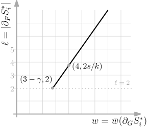
Figure 4.2: The line $\ell=g_{k,s}(w)$.

Now assume $s\geq(1.75+\Theta(\gamma))k$, and imagine the two-dimensional plane $\mathbb{R}^{2}$ where we plot the $(w,\ell)$ values for the different sets $S_{i}^{*}\in\mathcal{S}^{*}$ as points. The above discussion suggests a natural strategy of choosing a $S^{*}_{i}$, which is to draw a line with positive slope and choose $S^{*}_{i}$ corresponding to a point above the line. To guarantee the existence of a point above the line, we make sure that the lines pass the centroid of these $k$ points $(4,2s/k)$. Two points $(4,2s/k)$ and $(3-\gamma,2)$ (instead of $(3,2)$ for technical reasons) decide the following line.

$$\ell=g_{k,s}(w) :=\left(\left(\frac{2s}{k}-2\right)/\left(1+\gamma\right)\right)w+8/(1+\gamma)+\frac{s}{k}\left(2-8/(1+\gamma)\right)$$ (4.2)

$$=\left(\frac{2s}{k}-2-O(\gamma)\right)w+\left(8-\frac{6s}{k}+O(\gamma)\right).$$ (4.3)

See Figure 4.2. The line passes through the centroid $(4,2s/k)$, so we get the following statement, whose (easy) proof we omit:

Claim 4.2.

There exists a set $S^{*}_{i}$ such that $\ell\geq g_{k,s}(w)$.

(We handle the case $\ell<2$ separately, so only consider the segment from $\ell\geq 2$). Consider a $S^{*}_{i}$ whose $(w,\ell)$ point is above the line guaranteed by 4.2. Note that the line is above $(5,5)$ as long as $s\geq(1.75+\Theta(g))k$, and the slope is $\nicefrac{{2s}}{{k}}-2-O(\gamma)\geq 1.5-O(\gamma)$ so for large values of $w,\ell>5$, we have $w<\ell$, and the branching cost $O(n^{\beta})$ with $\beta=w$ by Lemma 2.2 is good. For small values, $\ell$ can be less than $w$, but our improved bounds Theorem 3.4 make sure that the branching factor is $O(n^{\beta})$ for $\beta<\ell$. In any case, our gain $\ell-\beta$ is strictly positive.

How do we analyze the performance of this algorithm? Suppose we run this process from $(k_{0},2k_{0}-2)$ and end up doing brute-force at the point $(k,s)$ with total gain $g$ over the entire process. This means that we have paid a total branching cost of $f(k)n^{(2k_{0}-2)-s-g}$ so far, leaving a forest $F$ with $\sum_{i}\ell\leq s$. We will then brute-force over the remaining $\leq s$ edges for a total running time of $f(k)n^{2k_{0}-2-g}$. Thus, to obtain the fastest $k_{0}$-cut possible, it is clear that our objective should be to maximize our total gain over the course of the process (which we can terminate at any point). Let us define the following quantity that measures how large $s$ is compared to $(1.75+\Theta(\gamma))k$.

$$z(k,s):=s-(1.75+\Theta(\gamma))k.$$ (4.4)

We can view $z$ as a budget that starts out as $(0.25-\Theta(\gamma))k_{0}$ and eventually becomes zero. We are interested in the amount of gain per unit of budget, which may depend on the current budget.

Recall that whenever $w\leq 14/3-\gamma$, our bounds in Theorem 3.4 provide better bounds than what is guaranteed in Lemma 2.2. We now formalize this below. Define the function

$$d(w):=\begin{cases}1&\text{if $w\leq 3-\gamma$},\\ 3-\nicefrac{{1}}{{4}}&\text{if $3-\gamma<w\leq 4-\gamma$},\\ 4-\nicefrac{{1}}{{4}}&\text{if $4-\gamma<w\leq\nicefrac{{14}}{{3}}-\gamma$, and}\\ w&\text{if $w>\nicefrac{{14}}{{3}}-\gamma$}.\end{cases}$$

By Theorem 3.4, if we branch on $(w,\ell)$, then the gain is $\ell-d(w)$ and the difference in budget is $z(k,s)-z(k-1,s-\ell)=\ell-(1.75+\Theta(\gamma))$. We now prove the lemma below that bounds the budget-gain ratio, whose proof is deferred to Appendix A.3.

Lemma 4.3.

Consider the current state $(k,s)$ with budget $z=z(k,s)=s-(1.75+\Theta(\gamma))k$, where $s\geq(1.75+\Theta(\gamma))k$, and $k\leq k_{0}$. Every point $(w,\ell)$ with $\ell\geq 2$ guaranteed by 4.2 satisfies

$$\frac{\ell-d(w)}{\ell-(1.75+\Theta(\gamma))}\geq\min\left(\frac{1}{9},\frac{4z}{6.5z+4.875k}(1-O(\gamma))\right)\geq\min\left(\frac{1}{9},\frac{4z}{6.5z+4.875k_{0}}(1-O(\gamma))\right).$$

Note that to handle the guessing of the coordinates $(w,\ell)$, the algorithm essentially guesses all values of $\ell$. Namely, for each integer value $\ell$, the algorithm enumerates all sets $A\subseteq V$ such that $(w(A),\ell)$ is on or above the line, which is good enough.

4.4 Correctness

We prove that $\ref{MinKCut}(G,k,F,s)$ finds every minimum $k$-cut that can be formed by deleting $s$ edges in $F$ and merging the $s+\kappa(F)$ connected components of $F$ into $k$ components. Fix any such minimum $k$-cut $\mathcal{S}^{*}$. If $s(k,s)<0$, then line 6 enumerates over all possible valid partitions, and hence $\mathcal{S}^{*}$ will be found. Otherwise, the following lemma shows that at least one component $S^{*}_{i}\in\mathcal{S}^{*}$ will be in $\mathcal{A}^{\ell}$ for some $\ell\in[0,s]$ so that we can recurse on $G\setminus S^{*}_{i}$ and eventually find $\mathcal{S}^{*}$.

Lemma 4.4.

If the else branch in LABEL:MinKCut is taken (i.e., $z(k,s)\geq 0\iff s\geq(1.75+\Theta(\gamma))k$), then there exists an $\ell\in[0,s]$ and $A\in\mathcal{A}^{\ell}$ such that $A\in\mathcal{S}^{*}$.

Proof.

If there exists $S^{*}_{i}$ whose $\ell$ is $0$ or $1$, $S^{*}_{i}\in\mathcal{A}^{\ell}$. When every $S^{*}_{i}$ has $\ell\geq 2$, by 4.2, there exists $S^{*}_{i}$ such that $\ell\geq g_{k,s}(w)\iff g^{-1}_{k,s}(\ell)\geq w$. If $\ell\geq 5$, $\beta_{\ell}=g^{-1}_{k,s}(\ell)\geq w$, and since $\mathcal{A}^{\ell}$ contains all cuts that crosses $F$ in $\ell$ edges and has weight at most $\beta_{\ell}$ in $G$, $S^{*}_{i}\in\mathcal{A}^{\ell}$. For $\ell=2,3,4$, let $\beta_{2}=3-\gamma$, $\beta_{3}=4-\gamma$, $\beta_{4}=14/3-\gamma$. Since $\ell\leq g_{k,s}(\beta_{\ell})\iff\beta_{\ell}\geq g_{k,s}^{-1}(\ell)$, so again $S^{*}_{i}\in\mathcal{A}^{\ell}$. ∎

4.5 Running Time

We now proceed to the running time analysis. Motivated by Lemma 4.3, we define the following potential function:

$$\Phi(k,s):=\begin{cases}\int_{t=0}^{z(k,s)}\min\left(\frac{1}{9},\frac{4t}{6.5t+4.875k_{0}}(1-\Theta(\gamma))\right)dt&\mbox{if }z(k,s)\geq 0\\ 1&\mbox{otherwise.}\end{cases}$$ (4.5)

The function has a discontinuity at $z(k,s)=0$, but this will be convenient later on. Below, we list the technical properties that we need for $\Phi$, whose routine proofs are deferred to Appendix A.3.

Lemma 4.5.

For values $(k,s)$ such that $z(k,s)\geq 0$, the function $\Phi(k,s)$ satisfies:

• $\Phi(k,s)\leq s$.

• $\Phi(k,s)\leq\Phi(k,s-1)+1$.

• $\Phi(k,s)\leq\min\{\Phi(k-1,s),\Phi(k-1,s-1)\}$.

• For all $(w,\ell)$ satisfying the condition in 4.2,

  $$\Phi(k,s)\leq\Phi(k-1,s-\ell)+\ell-d(w).$$

• $g_{k,s}^{-1}(s)\leq s-\Phi(k,s)+O(1)$.

The running time of LABEL:MinKCut is bounded by the following recursive analysis.

Lemma 4.6.

There exist $c_{1}=O(1)$ and $c_{2}=O(1/\gamma)$ such that Algorithm $\ref{MinKCut}(G,k,F,s)$ takes time

$$(c_{1}\,2^{k+s+\kappa(F)}))^{k}\cdot n^{s-\Phi(k,s)+c_{2}}.$$

Proof.

If $k<\Theta(1/\gamma)$, we take the if branch, and Karger-Stein takes time $O(n^{2k})=O(n^{O(1/\gamma)})$. This meets the bound for $c_{2}=O(1/\gamma)$, using that $\Phi(k,s)\leq s$ from Lemma 4.5.

If $s<(1.75+\Theta(\gamma))k$, we take the else if branch, and the enumeration on line 6 takes time

$$k^{s+\kappa(F)}n^{s+O(1)}\leq\big{(}2^{k+s+\kappa(F)}\big{)}^{k}\cdot n^{s-\Phi(k,s)+O(1)}.$$

Here, we use that if $z(k,s)<0$, then $\Phi(k,s)$ is defined to be $1$.

We now focus on the case $s\geq(1.75+\Theta(\gamma))k$, applying induction on $k$. Since all the recursive calls happen for each $A\in\mathcal{A}^{\ell}$ for some $\ell\in[0,s]$, we examine each $\mathcal{A}^{\ell}$ and bound the running time of the recursive calls based on $A\in\mathcal{A}^{\ell}$.

Recall that $\beta_{\ell}$ was defined to be $g_{k,s}^{-1}(\ell)$ for $\ell\geq 5$. Extend this definition so that $\beta_{0}=0,\beta_{1}=\beta_{2}=1,\beta_{3}=3-\nicefrac{{1}}{{4}},\beta_{4}=4-\nicefrac{{1}}{{4}}$. Observe the following:

1. $|\mathcal{A}^{\ell}|\leq O(2^{k}n^{\beta_{\ell}})$ by Lemma 2.2 and Theorem 3.4.

2. For every $A\in\mathcal{A}^{\ell}$ where $\ell\geq 0$, we define $s^{\prime}=s-|\partial_{F}A|$ and $F^{\prime}=F[V-A]$ in lines 16–17. This ensures that $s^{\prime}+\kappa(F^{\prime})\leq s+\kappa(F)$.

The number of recursive calls on line 18 is at most $|\mathcal{A}^{\ell}|$, and by induction, the recursive call corresponding to $A\in\mathcal{A}^{\ell}$ has runtime $(c_{1}2^{(k-1)+s^{\prime}+\kappa(F^{\prime})})^{k-1}\cdot n^{s^{\prime}-\Phi(k-1,s^{\prime})+c_{2}}$. The total time of these $|\mathcal{A}^{\ell}|\leq O(2^{k}n^{\beta_{\ell}})$ recursive calls for this value is $\ell$ is at most

$$O(2^{k}n^{\beta_{\ell}})\cdot(c_{1}2^{k+s+\kappa(F)})^{k-1}\cdot n^{s^{\prime}-\Phi(k-1,s^{\prime})+c_{2}}$$ (4.6)

Let us focus on the exponent of $n$ in this expression, $\beta_{\ell}+s^{\prime}-\Phi(k-1,s^{\prime})+c_{2}$. Lemma 4.5 shows that $\beta_{\ell}+s^{\prime}-\Phi(k-1,s^{\prime})\leq s-\Phi(k,s)$.

Substituting into (4.6), we get that for each $\ell\in[0,s]$, the recursive calls take total time

$$O(2^{k})\cdot(c_{1}2^{k+s+\kappa(F)})^{k-1}\cdot n^{s-\Phi(k,s)+c_{2}}.$$ (4.7)

Now to bound the time for the nonrecursive part of the algorithm. By the definition of LABEL:EnumCuts and Lemma 2.2, the runtime for lines 11 to 14 is dominated by the runtime for $\ref{EnumCuts}(G,\beta_{s},\infty)$, which is

$$n^{\beta_{s}+O(1)}\leq n^{s-\Phi(k,s)+c_{2}},$$ (4.8)

for large enough constant $c_{2}$, using item (6) of Lemma 4.5.

Using (4.7) to bound the time for recursive calls, and (4.8) for the non-recursive part, the total time of LABEL:MinKCut is at most

$$s\cdot O(2^{k})\cdot(c_{1}2^{k+s+\kappa(F)})^{k-1}\cdot n^{s-\Phi(k,s)+c_{2}}~{}~{}\leq~{}~{}(c_{1}2^{k+s+\kappa(F)})^{k}\cdot n^{s-\Phi(k,s)+c_{2}},$$

for large enough $c_{1}$. This completes the induction and finishes the lemma. ∎

Now using Thorup’s tree packing result from Theorem 2.1, we obtain an instance $(G,k_{0},F,s)$ with a single tree and hence $\kappa(F)=1$, where the optimal solution cuts this tree in at most $2k_{0}-2$ edges. We can try all choices of $s$ from $k_{0}-1$ to $2k_{0}-2$. By item (2) of Lemma 4.5, the value $s-\Phi(k_{0},s)$ is increasing in $s$, so the runtime will be maximum when $s=2k_{0}-2$. Our final running time is therefore

$$2^{O(k_{0}^{2})}\cdot n^{s-\Phi(k_{0},2k_{0}-2)+O(1)}.$$

It remains to compute $\Phi(k_{0},2k_{0}-2)$. If we let $f(t):=\min\left(\frac{1}{9},\frac{4t}{6.5t+4.875k_{0}}(1-\Theta(\gamma))\right)$, then the two terms inside the $\min(\cdot,\cdot)$ are equal when $t$ equals $T:=\frac{4.875}{29.5(1-\Theta(\gamma))}k_{0}$. That is, $f(t)=1/9$ for $t\geq\frac{4.875}{29.5(1-\Theta(\gamma))}k_{0}$ and $f(t)=\frac{4t}{6.5t+4.875k_{0}}(1-\Theta(\gamma))$ otherwise. Integrating $\Phi(k_{0},s)$ for $z=z(k_{0},s)<k_{0}T$, we obtain

$$\Phi(k_{0},s)=\int_{t=0}^{z}\frac{4t}{6.5t+4.875k_{0}}(1-\Theta(\gamma))=\frac{(1-\Theta(\gamma))}{1.625}(z/k_{0}-0.75\ln(4z/k_{0}+3)+0.75\ln 3)k_{0}.$$

Therefore, for a value of $s$ satisfying $z(k_{0},s)>k_{0}T$, we have

$$\Phi(k_{0},s)=\frac{(1-\Theta(\gamma))}{1.625}(T-0.75\ln(4T+3)+0.75\ln 3)k_{0}+\frac{1}{9}(z-k_{0}T).$$

Plugging in $s:=2k_{0}-2$, we obtain

$$\Phi(k_{0},2k_{0}-2) =\frac{1}{1.625}\cdot\left(\frac{4.875}{29.5}-0.75\ln\left(4\cdot\frac{4.875}{29.5}+3\right)+0.75\ln 3\right)k_{0}+\frac{1}{9}\left(0.25k_{0}-\frac{4.875}{29.5}k_{0}\right)-O(\gamma k_{0})$$

$$\approx(0.0192055688-O(\gamma))k_{0}.$$

Assuming that $k_{0}$ is large enough, set $\gamma>0$ so that

$$s-\Phi(k_{0},2k_{0}-2)+O(1)\approx(2k_{0}-2)-(0.0192055688-O(\gamma))k_{0}+O(1)\leq 1.981k_{0}.$$

Finally, plugging in this bound of $s-\Phi(k_{0},2k_{0}-2)+O(1)$ into Lemma 4.6 proves Theorem 1.1.

5 The Extremal Problem

In this section we will prove the extremal theorems (Theorems 3.2 and 3.3) from §3.2 about the size of certain set systems that do not have certain intersection patterns. The results of this section may be read independently of the other sections, if desired.

Since we will be talking about two kinds of sets, one over a universe $X$ and another over a small universe $[k]$, we use the vocabulary of range spaces commonly used in the computational and discrete geometry literature. A range space $(X,\mathcal{R})$ is just a set system over the ground set $X$, where the sets in $\mathcal{R}$ are called ranges. The following notion of representation will be useful to state our results formally and concisely: please refer to Figure 5.3 as well.

Definition 5.1 (Represent).

Let $X$ be a universe of elements. Let $k\in\mathbb{N}$ be a positive integer and $\mathcal{S}\subseteq 2^{[k]}$ be a set of subsets of $[k]$. For given ranges $R_{1},\ldots,R_{k}\subseteq X$ and subset $S\in\mathcal{S}$, we say that $R_{1},\ldots,R_{k}$ witnesses $(k,S)$ if there exists element $x\in X$ such that for all indices $i\in[k]$,

$$i\in S\iff x\in R_{i}.$$

We say that a $k$-tuple of ranges $(R_{1},\ldots,R_{k})$ $\alpha$-witnesses $(k,\mathcal{S})$ in $X$ if they witness at least an $\alpha$-fraction of subsets $S\in\mathcal{S}$. We drop the “in $X$” if the universe $X$ is clear from context.

Now consider a range space $(X,\mathcal{R})$. We say that $\mathcal{R}$ $\alpha$-represents $(k,\mathcal{S})$ in $X$ if there exists subsets $R_{1},\ldots,R_{k}\in\mathcal{R}$ that $\alpha$-witness $\mathcal{S}$.

Figure 5.3: A Venn diagram representation of three ranges $R_{1},R_{2},R_{3}$ on a universe $X$ of $8$ elements. The tuple $(R_{1},R_{2},R_{3})$ $\nicefrac{{5}}{{8}}$-witnesses $(3,2^{[3]})$, $\nicefrac{{4}}{{7}}$-witnesses $(3,2^{[3]}\backslash\{\varnothing\})$, and $1$-witnesses $(3,\{\varnothing,\{1\},\{3\},\{1,2\},\{1,2,3\}\})$.

Again, Figure 5.3 may be useful in understanding the notion. Readers familiar with the notion of VC-dimension will recognize that if some range space $(X,\mathcal{R})$ $1$-represents the set system $(k,2^{[k]})$, this corresponds to the dual range space $(\mathcal{R},\mathcal{R}^{*})$ having VC dimension at least $k$. The notion of witnesses and representation we define above is therefore a more refined notion than the usual notion of (dual) shattering. While we do not need familiarity with any of these connections, we refer to, e.g., [Mat99, §5.1] for more details on VC dimension and dual shatter functions.

Claim 5.2.

Let $(X,\mathcal{R})$ be a range space with $|X|=n$. If $|\mathcal{R}|>2n-2$ then there exist two ranges in $\mathcal{R}$ that cross.

In this section, we prove Theorems 3.2 and 3.3 on extremal set bounds. First, let us restate them in terms of the above notation.

Theorem 5.3 ($\nicefrac{{7}}{{8}}$-representation).

Let $(X,\mathcal{R})$ be a range space with $|X|=n$. There exists a positive constant $c$ such that if $|\mathcal{R}|>cn^{3-1/4}$, then $\mathcal{R}$ $\nicefrac{{7}}{{8}}$-represents $(3,2^{[3]})$.

Theorem 5.4 ($1$-representation).

Let $(X,\mathcal{R})$ be a range space with $|X|=n$. There exists a positive constant $c$ such that if $|\mathcal{R}|>cn^{4-1/4}$, then $\mathcal{R}$ $1$-represents $(3,2^{[3]})$.

We can rephrase Theorem 5.4 in terms of the concept dual VC dimension from VC dimension theory. The following is a simple, equivalent definition of dual VC dimension in terms of our notion of representation:

Definition 5.5 (Dual VC dimension).

A range space $(X,\mathcal{R})$ has dual VC dimension $d$ if $d$ is the largest integer such that $\mathcal{R}$ $1$-represents $(d,2^{[d]})$.

Thus, 5.4 implies the following extremal bound concerning range spaces of dual VC dimension at least $3$:

Corollary 5.6.

Let $(X,\mathcal{R})$ be a range space with $|X|=n$. There exists a positive constant $c$ such that if $|\mathcal{R}|>cn^{4-1/4}$, then $\mathcal{R}$ has dual VC dimension at least $3$.

We first develop some basic tools in §5.1 to give weaker results; the proofs of the above theorems then appear in §5.2. Before we proceed, here are some standard notions and a basic result about the maximum number of sets in a laminar set system.

Definition 5.7 (Crossing Sets).

Let $X$ be a universe of elements. We say that two ranges $A,B\subseteq X$ cross in $X$ if $(A,B)$ $1$-witnesses $(2,2^{[2]})$ in $X$. That is, there is at least one element in each of the sets $A\backslash B$, $B\backslash A$, $A\cap B$, and $\overline{A\cup B}$.

Definition 5.8 (Cutting Sets).

Let $X$ be a universe of elements. We say that range $A$ cuts range $B$ if there is an element in each of the sets $A\cap B$ and $B\backslash A$.

Using these definitions, we can easily prove Claim 5.2 restated below.

See 5.2

Proof.

Fix an arbitrary element $x\in X$. Let $\mathcal{R}^{\prime}$ be the set $\{R:R\in\mathcal{R},x\notin R\}\cup\{\overline{R}:R\in\mathcal{R},x\in R\}$, so that $(X\backslash\{x\},\mathcal{R}^{\prime})$ is a range space. We have $|\mathcal{R}^{\prime}|\geq|\mathcal{R}|/2$, since for every pair of ranges $R,\overline{R}$ satisfying $\{R,\overline{R}\}\cap\mathcal{R}\neq\varnothing$, one of $R,\overline{R}$ is in $\mathcal{R}^{\prime}$. Since $|\mathcal{R}^{\prime}|\geq|\mathcal{R}|/2>n-2=|X\backslash\{x\}|-1$, $\mathcal{R}^{\prime}$ is not a laminar set of ranges, so there exist $A,B\in\mathcal{R}^{\prime}$ such that $A\backslash B$, $B\backslash A$, and $A\cap B$ are nonempty. Since $x\in\overline{A\cup B}$, the sets $A,B$ cross in $X$. It is easy to see that any of $(A,\overline{B})$, $(\overline{A},B)$, and $(\overline{A},\overline{B})$ also cross in $X$. Since for one of these pairs, both ranges are in $R$, the claim follows. ∎

5.1 Warm-up

In this section, we prove simpler results while developing some basic machinery. The ideas here are similar to those used, e.g., in proofs of the Sauer-Shelah theorem about the VC dimension of set systems.

Lemma 5.9 (Extension Lemma).

Let $(X,\mathcal{R})$ be a range space with $|X|=n$. Suppose the following statement is true, for some fixed constant $c$, nonnegative integers $d,k,r$, and subset $\mathcal{S}\subseteq 2^{[k]}$ with $r<|\mathcal{S}|$:

• If $|\mathcal{R}|>cn^{d}$, then $\mathcal{R}$ $(\nicefrac{{r}}{{|\mathcal{S}|}})$-represents $(k,\mathcal{S})$.

Then there exists constant $c^{\prime}$ depending on $c,d$ such that the following statement is also true:

• If $|\mathcal{R}|>c^{\prime}n^{d+1}$, then $\mathcal{R}$ $(\nicefrac{{r+1}}{{|\mathcal{S}|}})$-represents $(k,\mathcal{S})$.

Proof.

It suffices to prove statement (2) for $n$ large enough: by setting $c^{\prime}\geq 2^{n_{0}}$ for some $n_{0}\geq 0$, the statement is true for all $n\leq n_{0}$, since $|\mathcal{R}|>c^{\prime}n^{d+1}$ is impossible if $|X|\leq n_{0}$.

We apply induction for large enough $n$. Pick an arbitrary $x\in X$, and let $\mathcal{R}_{\textup{both}}$ be the set of all $R$ satisfying $R\not\ni x$, $R\in\mathcal{R}$, and $R\cup\{x\}\in\mathcal{R}$.

First, suppose that $|\mathcal{R}_{\textup{both}}|>cn^{d}$. Then, by the assumption in the lemma, there exists a $r/|\mathcal{S}|$-witness $(R_{1},R_{2},\ldots,R_{k})$ for $(k,\mathcal{S})$. If $(R_{1},R_{2},\ldots,R_{k})$ also $(r+1)/|\mathcal{S}|$-witnesses $(k,\mathcal{S})$, then we are done; otherwise, let $S^{*}\in\mathcal{S}$ be a subset not witnessed by $(R_{1},R_{2},\ldots,R_{k})$. For each $i\in[k]$, define $R^{\prime}_{i}$ to be $R_{i}$ if $x\notin S^{*}$, and $R_{i}\cup\{x\}$ otherwise; note that $R^{\prime}_{i}\in\mathcal{R}$ always. Then, every subset $S\in\mathcal{S}$ witnessed by $(R_{1},R_{2},\ldots,R_{k})$ is also witnessed by $(R_{1}^{\prime},R_{2}^{\prime},\ldots,R_{k}^{\prime})$, and moreover, $S^{*}$ is now witnessed by $(R_{1}^{\prime},R_{2}^{\prime},\ldots,R_{k}^{\prime})$. Therefore, $(R_{1}^{\prime},R_{2}^{\prime},\ldots,R_{k}^{\prime})$ $(r+1)/|\mathcal{S}|$-represents $(k,\mathcal{S})$.

Otherwise, suppose that $|\mathcal{R}_{\textup{both}}|\leq cn^{d}$. Define $\mathcal{R}_{\textup{one}}$ to be the set of all $R$ satisfying $R\not\ni x$ and exactly one of $R\in\mathcal{R}$ and $R\cup\{x\}\in\mathcal{R}$; observe that $|\mathcal{R}_{\textup{one}}|+2\cdot|\mathcal{R}_{\textup{both}}|=|\mathcal{R}|$, and that $(X\backslash x,\mathcal{R}_{\textup{one}}\uplus\mathcal{R}_{\textup{both}})$ is a range space with $|X\backslash x|=n-1$. If there exists a $(r+1)/|\mathcal{S}|$-witness for $\mathcal{R}_{\textup{one}}\uplus\mathcal{R}_{\textup{both}}$, then clearly, this tuple also $(r+1)/|\mathcal{S}|$-witnesses $\mathcal{R}$, so assume not. Applying induction on the contrapositive of statement (2) gives $|\mathcal{R}_{\textup{one}}\uplus\mathcal{R}_{\textup{both}}|\leq c^{\prime}(n-1)^{d+1}$. Therefore,

$$|\mathcal{R}|=|\mathcal{R}_{\textup{one}}\uplus\mathcal{R}_{\textup{both}}|+|\mathcal{R}_{\textup{both}}| \leq c^{\prime}(n-1)^{d+1}+cn^{d}$$

$$\leq c^{\prime}n^{d+1}-c^{\prime}\cdot Cn^{d}+cn^{d},$$

for some constant $C\geq 0$ depending on $d$, and assuming that $n$ is large enough. Setting $c^{\prime}\geq c/C$ gives

$$|\mathcal{R}|\leq c^{\prime}n^{d+1}-c^{\prime}\cdot Cn^{d}+cn^{d}\leq c^{\prime}n^{d+1},$$

so the assumption of statement (2) is false, completing the induction. ∎

Lemma 5.10.

Let $(X,\mathcal{R})$ be a range space with $|X|=n$. There exists constants $c_{1},c_{2},c_{3},c_{4}$ such that:

• If $|\mathcal{R}|>c_{1}n$, then $\mathcal{R}$ $\nicefrac{{5}}{{8}}$-represents $(3,2^{[3]})$.

• If $|\mathcal{R}|>c_{2}n^{2}$, then $\mathcal{R}$ $\nicefrac{{6}}{{8}}$-represents $(3,2^{[3]})$.

• If $|\mathcal{R}|>c_{3}n^{3}$, then $\mathcal{R}$ $\nicefrac{{7}}{{8}}$-represents $(3,2^{[3]})$.

• If $|\mathcal{R}|>c_{4}n^{4}$, then $\mathcal{R}$ $1$-represents $(3,2^{[3]})$.

Proof.

We first prove (1). Let $c_{1}:=16$. Since $|\mathcal{R}|>16n$, there exists $A,B$ that cross, by Claim 5.2. If $C$ is any set other than the union of some subset of $\{A\backslash B,B\backslash A,A\cap B,\overline{A\cup B}\}$, then $(A,B,C)$ is a $\nicefrac{{5}}{{8}}$-witness for $(3,2^{[3]})$. There are at most $2^{4}=16$ such unions and $|\mathcal{R}|>16n\geq 16$, so there is such a choice for $C$.

This serves as the base case: we can now use the Extension Lemma above: Statement (2) follows from (1) and an application of Lemma 5.9 with $d:=1$, $k:=3$, $r:=5$, and $\mathcal{S}:=2^{[3]}$. Likewise, statement (3) follows from (2) with $d:=2$ and $r:=6$, and statement (4) follows from (3) with $d:=3$ and $r:=7$. ∎

Observe that statement (4) of Lemma 5.10 is weaker than Theorem 5.4 by an $n^{1/4}$ factor. If we were to stick to the proof strategy in Lemma 5.10, we would want to prove improved statements (1) to (3) in order to get an improved statement (4). However, statements (1) and (2) of Lemma 5.10 are tight, and become false if we replace $|\mathcal{R}|\geq c_{d}n^{d}$ with $|\mathcal{R}|\geq c_{d}n^{d-\varepsilon}$ for $d=1,2$ and some $\varepsilon>0$. For example, if $\mathcal{R}$ is all ranges of size $2$ in $X$, then $\mathcal{R}$ has size $\binom{n}{2}$ but still does not $\nicefrac{{6}}{{8}}$-represent $(3,2^{[3]})$. However, statement (3) does not suffer from a simple, matching lower bound, and indeed, as promised by Theorem 5.3, the bound can be improved by $n^{1/4}$. Our main focus will be to prove this improved upper bound on statement (3), from which the improved statement (4) from Theorem 5.4 will follow.

5.2 Proof of the Extremal Theorems

The main idea behind our improved proofs is prove statements that give a finer-grained control over the occupied regions of the Venn diagrams. Since some regions of the Venn diagram are “easy” to achieve (say the intersection of all sets, or the complement of their union), we seek results that show that with enough sets, there exist three sets such that many of the “difficult” regions are occupied.

For example, the first structure lemma shows that with linear number of sets, one can have four Venn diagram regions be occupied. Note that statement (1) of Lemma 5.10 already showed how to achieve five out of eight regions. But the lemma below ensures that the four occupied regions do not include the “easy” regions $[3]$ or $\varnothing$; this makes the proof considerably more technical. (We defer its somewhat unedifying proof to §5.2.1.)

Lemma 5.11 (First Structure Lemma).

Let $(X,\mathcal{R})$ be a range space with $|X|=n$. There exists positive constant $c$ such that if $|\mathcal{R}|>cn$, then $\mathcal{R}$ $\nicefrac{{4}}{{6}}$-represents $(3,2^{[3]}\backslash\{\varnothing,[3]\})$.

Corollary 5.12.

Let $(X,\mathcal{R})$ be a range space with $|X|=n$. There exists positive constant $c$ such that if $|\mathcal{R}|\geq cn^{2}$, then $\mathcal{R}$ $\nicefrac{{5}}{{6}}$-represents $(3,2^{[3]}\backslash\{\varnothing,[3]\})$.

Proof.

Start with Lemma 5.11 and apply the Extension Lemma 5.9 with parameters $d:=1$, $k:=3$, $r:=4$, and $\mathcal{S}:=2^{[3]}\backslash\{\varnothing,[3]\}$. ∎

The next structure lemma is again in the same vein: the statement is similar to statement (2) of Lemma 5.10, and in fact seems quantitatively worse. (It requires a large number of ranges, and also that ranges have small size.) But again it does not require the “easy” set $\varnothing$ to be represented; we will use this flexibility soon.

Lemma 5.13 (Second Structure Lemma: Small Sizes).

Let $(X,\mathcal{R})$ be a range space with $|X|=n$, and let $\varepsilon\leq 1$ be a positive constant. Suppose that every range $R\in\mathcal{R}$ satisfies $|R|\leq n^{\varepsilon}$. Then, there exists positive constant $c$ such that if $|\mathcal{R}|\geq cn^{2+3\varepsilon}$, then $\mathcal{R}$ $(\nicefrac{{6}}{{7}})$-represents $(3,2^{[3]}\backslash\{\varnothing\})$.

Proof.

The idea of the proof is very natural: since the ranges are small, we can pick a range $A$ and restrict our attention to the intersections of other ranges with $A$. If there are many distinct intersections in this small sub-universe, we inductively get our result. Else there are few distinct intersections, so on average there are a lot of ranges $R$ that give the same intersections $R\cap A$. Now we can argue about how the other ranges intersect $A$ and $\overline{A}$ to prove the result.

For convenience, define $s:=n^{\varepsilon}$. Suppose that $|\mathcal{R}|\geq cn^{2+3\varepsilon}=cn^{2}s^{3}$; we will set the constant $c$ later. Consider a complete graph $G=(X,E)$ whose vertices are the elements of $X$. We abuse notation, sometimes referring to an edge $(u,v)\in E$ as the two-element set $\{u,v\}\subseteq X$. Call an edge $e=\{u,v\}$ light if $e$ is contained in $\leq cs^{3}$ many ranges in $\mathcal{R}$, and heavy otherwise. Also, call a range in $\mathcal{R}$ light if it contains a light edge, and heavy otherwise.

While there exists a light range, remove it from $\mathcal{R}$, after which some ranges that were previously heavy may become light. We claim that we can remove at most $\binom{n}{2}\cdot cs^{3}$ ranges from this iterative operation. For each light range removed, charge it to an arbitrary edge inside it that was light when the range was removed. The first time an edge $e$ is charged, it must be light, so $e$ is contained in at most $cs^{3}$ ranges before it is first charged. Every charge to $e$ reduces the number of ranges containing $e$ by $1$, so edge $e$ is charged at most $cs^{3}$ times. There are $\binom{n}{2}$ edges, leading to at most $\binom{n}{2}\cdot cs^{3}$ charges, completing the claim.

Since $|\mathcal{R}|\geq cn^{2}s^{3}>\binom{n}{2}\cdot cs^{3}$, there are still ranges left, all of which are heavy; we now work with only these remaining ranges. Let $A$ be a (remaining heavy) range of maximal size. For each subset $S\subseteq A$, declare a bucket labeled with $S$. For each range $R$ with $R\cap A\neq\varnothing$, add it into the bucket labeled with $R\cap A$. Let $\mathcal{R}_{A}\subseteq 2^{A}$ be the set of labels on nonempty buckets, and let $\mathcal{R}_{A}^{+}\subseteq 2^{A}$ be the set of labels on buckets of size at least $3$.

First, suppose that $|\mathcal{R}_{A}^{+}|>2s\geq 2(|A|-2)$. Then, there exists nonempty buckets $B_{1},B_{2}\in\mathcal{R}_{A}^{+}$ that cross. Pick a range $R_{1}\in B_{1}$ with $R_{1}\neq B_{1}$; we can find such a range since bucket $B_{1}$ has size at least $2$. Pick a range $R_{2}\in B_{2}$ with $R_{2}\neq B_{2}$ and $R_{2}\backslash A\neq R_{1}\backslash A$; we can find such a range since bucket $B_{2}$ has size at least $3$. Now consider the tuple $(R_{1},R_{2},A)$. Since $B_{1},B_{2}$ cross, $(R_{1},R_{2},A)$ $1$-represents $(3,\{\{3\},\{1,3\},\{2,3\},\{1,2,3\}\})$. Moreover, by choice of $R_{1},R_{2}$ inside buckets $B_{1},B_{2}$, $(R_{1},R_{2},A)$ also $2/3$-represents $(3,\{\{1\},\{2\},\{1,2\}\})$. Thus, $(R_{1},R_{2},A)$ $\nicefrac{{6}}{{7}}$-represents $(3,2^{[3]}\backslash\{\varnothing\})$.

From now on, assume that $|\mathcal{R}_{A}^{+}|\leq 2s$. By Lemma 5.10 on range space $(A,\mathcal{R}_{A})$, there exists constant $c_{3}$ such that if $|\mathcal{R}_{A}|>c_{3}\cdot|A|^{3}$, then there exists $(A_{1},A_{2},A_{3})$ that $\nicefrac{{7}}{{8}}$-witnesses $(3,2^{[3]})$ in $A$. In particular, if this is the case, then $(A_{1},A_{2},A_{3})$ $\nicefrac{{6}}{{7}}$-witnesses $(3,2^{[3]}\backslash\{\varnothing\})$ in $A$. For each $A_{i}$, let $R_{i}\in\mathcal{R}$ be a range in bucket $A_{i}$. Then, $(R_{1},R_{2},R_{3})$ $\nicefrac{{6}}{{7}}$-witnesses $(3,2^{[3]}\backslash\{\varnothing\})$ in $R$, as desired.

Therefore, we can assume that the number of nonempty buckets, $|\mathcal{R}_{A}|$, is at most $c_{3}\cdot|A|^{3}\leq c_{3}s^{3}$. Call a bucket frequent if it has at least $((c-2c_{3})/2)s^{2}$ ranges inside it.

Claim 5.14.

For every $e\in G[A]$, there is a frequent bucket containing $e$.

Proof.

For each edge $e$ in $G[A]$, since $e$ is heavy, it is contained in at least $cs^{3}$ many ranges. Since $|\mathcal{R}_{A}\backslash\mathcal{R}_{A}^{+}|\leq|\mathcal{R}_{A}|\leq c_{3}s^{3}$, at most $c_{3}s^{3}\cdot 2$ ranges belong to a bucket in $\mathcal{R}_{A}\backslash\mathcal{R}_{A}^{+}$. This leaves at least $(c-2c_{3})s^{3}$ ranges that belong to buckets in $\mathcal{R}_{A}^{+}$, and since $|\mathcal{R}_{A}^{+}|\leq 2s$, there must be a frequent bucket (in $\mathcal{R}_{A}^{+}$) containing $e$. This proves the claim. ∎

Figure 5.4: The construction of $B_{1},B_{2},B_{3},u,v,w$.

Of all frequent buckets, let $B_{1}$ be (the label of) the frequent bucket with maximum value of $|B_{1}|$. We know that $B_{1}\neq A$, since the bucket labeled $A$ only has one range, namely $A$, so it is not frequent. Fix two vertices $u\in B_{1}$ and $v\in A\backslash B_{1}$, and let $B_{2}$ be a frequent bucket containing edge $(u,v)$; note that $B_{2}\neq B_{1}$. Since $B_{1}$ is the frequent bucket with maximum $|B_{1}|$, $B_{1}$ is not contained in $B_{2}$, so there is a vertex $w$ in $B_{1}\backslash B_{2}$. Let $B_{3}$ be a frequent bucket containing edge $(v,w)$. See Figure 5.4.

Observe that $(B_{1},B_{2},B_{3})$ $3/4$-witnesses $(3,\{\{1,3\},\{2,3\},\{1,2\},\{1,2,3\}\})$ in $A$. Namely, $w\in B_{1}\cap\overline{B_{2}}\cap B_{3}$ and $v\cap\overline{B_{1}}\cap B_{2}\cap B_{3}$ fulfill $\{1,3\}$ and $\{2,3\}$ respectively, and $u\in B_{1}\cap B_{2}$ fulfills either $\{1,2\}$ or $\{1,2,3\}$.

Claim 5.15.

There exist ranges $R_{1},R_{2},R_{3}\in\mathcal{R}$ such that $R_{i}\cap A=B_{i}$ for each $i\in[3]$ and $(R_{1}\backslash A,R_{2}\backslash A,R_{3}\backslash A)$ $1$-witnesses $(3,\{\{1\},\{2\},\{3\}\})$ in $X\backslash A$.

Proof.

For each $i\in[3]$, pick a random range from the frequent bucket $B_{i}$. For $i\in[3]$, define event $\textsf{Bad}_{i}$ to be the event that $R_{i}\backslash A\subseteq\bigcup_{j\neq i}(R_{j}\backslash A)$. It is clear that if no event $\textsf{Bad}_{i}$ holds, then $(R_{1}\backslash A,R_{2}\backslash A,R_{3}\backslash A)$ $1$-witnesses $(3,\{\{1\},\{2\},\{3\}\})$ in $X\backslash A$.

To bound $\Pr[\textsf{Bad}_{1}]$, fix ranges $R_{2},R_{3}$. Since all ranges $R$ in bucket $B_{1}$ satisfy $R\cap A=B_{1}$, the values $R\backslash A$ are all distinct. By Corollary 5.12, there exists constant $c_{2}$ such that if at least $c_{2}|R_{2}\cup R_{3}|^{2}$ many such values $R\backslash A$ are contained in $R_{2}\cup R_{3}$, then there exist ranges $R_{1}^{\prime},R_{2}^{\prime},R_{3}^{\prime}$ in bucket $B_{1}$ such that $(R_{1}^{\prime}\backslash A,R_{2}^{\prime}\backslash A,R_{3}^{\prime}\backslash A)$ $\nicefrac{{5}}{{6}}$-represents $(3,2^{[3]}\backslash\{\varnothing,[3]\})$ in $X\backslash A$. Since $R^{\prime}_{1}\cap R^{\prime}_{2}\cap R^{\prime}_{3}\supseteq B_{1}\neq\varnothing$, $(R_{1}^{\prime},R_{2}^{\prime},R_{3}^{\prime})$ $\nicefrac{{6}}{{7}}$-represents $(3,2^{[3]}\backslash\{\varnothing\})$ in $X$, proving the lemma. Therefore, we may assume that there are less than $c_{2}|R_{2}\cup R_{3}|^{2}\leq c_{2}(2s)^{2}$ many values $R\backslash A$ for range $R$ in bucket $B_{1}$ that satisfy $R\backslash A\subseteq R_{2}\cup R_{3}$. The frequent bucket $B_{1}$ has at least $((c-2c_{3})/2)s^{2}$ ranges, so as long as we have

$$((c-2c_{3})/2)s^{2}>3c_{2}(2s)^{2}\iff c>24c_{2}^{2}+2c_{3},$$

we have

$$\Pr[\textsf{Bad}_{1}\text{ given choice of }R_{2},R_{3}]=\Pr[R_{1}\subseteq R_{2}\cup R_{3}\text{ given choice of }R_{2},R_{3}]<\frac{1}{3}.$$

Since $R_{2},R_{3}$ are arbitrary ranges, we have $\Pr[\textsf{Bad}_{1}]<1/3$. Repeating the argument for the other two buckets gives $\Pr[\textsf{Bad}_{i}]<1/3$ for all $i\in[3]$. Thus, the probability of a bad event is strictly less than $1$, so there is a satisfying choice of $R_{1},R_{2},R_{3}$. ∎

Thus, the choice of $(R_{1},R_{2},R_{3})$ in Claim 5.15 both $3/4$-witnesses $(3,\{\{1,3\},\{2,3\},\{1,2\},\{1,2,3\}\})$ in $A$ and $1$-witnesses $(3,\{\{1\},\{2\},\{3\}\})$ in $X\setminus A$, so it is a $\nicefrac{{6}}{{7}}$-witness for $(3,2^{[3]}\backslash\{\varnothing\})$, proving the lemma. ∎

Recall that the Second Structure Lemma 5.13 required the sets to have small sizes. We now give the easy extension to handle all sizes of sets.

Lemma 5.16 (Second Structure Lemma: General Sizes).

Let $(X,\mathcal{R})$ be a range space with $|X|=n$. There exists a positive constant $c$ such that if $|\mathcal{R}|>cn^{3-1/4}$, then $\mathcal{R}$ $\nicefrac{{6}}{{7}}$-represents $(3,2^{[3]}\backslash\{\varnothing\})$.

Proof.

Set $\varepsilon:=\nicefrac{{1}}{{4}}$. Call a range in $\mathcal{R}$ small if its size is at most $n^{\varepsilon}$, and large otherwise, and let $\mathcal{R}_{\textup{small}}$ and $\mathcal{R}_{\textup{large}}$ be the small and large ranges, respectively. If $|\mathcal{R}_{\textup{small}}|>(c/2)n^{3-\varepsilon}$, then applying Lemma 5.13 on $\mathcal{R}_{\textup{small}}$ proves the lemma, assuming that $c$ is large enough. Otherwise, $|\mathcal{R}_{\textup{large}}|>(c/2)n^{3-\varepsilon}$. If so, there is some element $x\in X$ that is in more than $(c/2)n^{3-\varepsilon}\cdot n^{\varepsilon}/n=(c/2)n^{2}$ many large ranges. Let $\mathcal{R}_{\textup{large}}^{x}$ be these large ranges; by Corollary 5.12, if $c$ is large enough, then there is tuple $(R_{1},R_{2},R_{3})$ of ranges in $\mathcal{R}^{\prime}$ that $\nicefrac{{5}}{{6}}$-witnesses $(3,2^{[3]}\backslash\{\varnothing,[3]\})$. Since $x\in R_{1}\cap R_{2}\cap R_{3}$, the tuple $\nicefrac{{6}}{{7}}$-witnesses $(3,2^{[3]}\backslash\{\varnothing\})$, as desired. ∎

Having proved the structure lemmas, we can turn to proving the main theorems of this section. We first prove Theorem 5.3, restated below. (This improves on statement (3) of Lemma 5.10.)

See 5.3

Proof.

Set $c:=2c^{\prime}$, where $c^{\prime}$ is the constant in Lemma 5.16, and suppose that $|\mathcal{R}|>cn^{3-1/4}$. Following the proof of Claim 5.2, fix an arbitrary element $x\in X$, and let $\mathcal{R}^{\prime}$ be the set $\{R:R\in\mathcal{R},x\notin R\}\cup\{\overline{R}:R\in\mathcal{R},x\in R\}$, so that $(X\backslash\{x\},\mathcal{R}^{\prime})$ is a range space. We have $|\mathcal{R}^{\prime}|\geq|\mathcal{R}|/2>c^{\prime}n^{3-1/4}$, since for every pair of ranges $R,\overline{R}$ satisfying $\{R,\overline{R}\}\cap\mathcal{R}\neq\varnothing$, one of $R,\overline{R}$ is in $\mathcal{R}^{\prime}$. By the Second Structure Lemma 5.16, there exists ranges $R_{1},R_{2},R_{3}$ such that $(R_{1},R_{2},R_{3})$ $\nicefrac{{6}}{{7}}$-witnesses $(3,2^{[3]}\backslash\{\varnothing\})$ in $X\backslash\{x\}$. Since $x\in\overline{R_{1}\cup R_{2}\cup R_{3}}$, $(R_{1},R_{2},R_{3})$ also $\nicefrac{{7}}{{8}}$-witnesses $(3,2^{[3]})$ in $X$. Finally, one of the eight tuples obtained by taking or not taking the complement of each $R_{i}$ gives a tuple of ranges in $\mathcal{R}$ that also $\nicefrac{{7}}{{8}}$-witnesses $(3,2^{[3]})$, proving the theorem. ∎

An application of the Extension Lemma to the above result proves Theorem 5.4, restated below.

See 5.4

Proof.

Starting with Theorem 5.3, apply the Extension Lemma 5.9 with parameters $d:=3-1/4$, $k:=3$, $r:=7$, and $\mathcal{S}:=2^{[3]}$. ∎

5.2.1 Deferred Proofs

Proof of Lemma 5.11.

The proof has many cases; see Figure 5.5 for a visualization of some of the cases.

We induct on $n$, with the case $n=1$ being trivial as long as $c\geq 2$, since $|\mathcal{R}|>2n$ is impossible if $|X|=1$.

Figure 5.5: Illustration of some of the cases for the proof of Lemma 5.11.

Assuming that $c\geq 2$, we have $|R|>2n$, so there exist ranges $A,B\in\mathcal{R}$ that cross. Let $A,B$ be the two crossing sets with minimum $|A\cap B|$. Fix arbitrary elements $a\in A\backslash B$, $b\in B\backslash A$, and $d\in\overline{A\cup B}$.

1. If no range $R\in\mathcal{R}$ contains $d$, then remove $d$ from $X$ and apply induction. More formally, set $X^{\prime}:=X\backslash\{d\}$; since $(X^{\prime},\mathcal{R})$ is still a range space, we have $|\mathcal{R}|\leq c|X^{\prime}|$ by induction, so $|\mathcal{R}|\leq c|X|$.

2. If some range $C\ni d$ satisfies $C\not\supseteq A\cap B$, then the set $(A,B,C)$ works, i.e., it $\nicefrac{{4}}{{6}}$-represents $(3,2^{[3]}\backslash\{\varnothing,[3]\})$. This is because $a$ fulfills either $\{1\}$ or $\{1,3\}$, $b$ fulfills either $\{2\}$ or $\{2,3\}$, $d$ fulfills $\{3\}$, and there is some element $c^{\prime}\in(A\cap B)\backslash C$ that fulfills $\{1,2\}$.

3. If some range $C\ni d$ cuts $A\backslash B$, then the set $(A,B,C)$ works, because $b$ fulfills either $\{2\}$ or $\{2,3\}$, $d$ fulfills $\{3\}$, and there are elements $c_{1}\in(A\backslash B)\cap C$ and $c_{2}\in(A\backslash B)\backslash C$ that fulfill $\{1,3\}$ and $\{1\}$, respectively.

4. If some range $C\ni d$ cuts $B\backslash A$, then the set $(A,B,C)$ works by a symmetric argument.

If any element $d\in\overline{A\cup B}$ satisfies (2), (3), or (4), then we are done, so we may assume that none of them do. This implies the following assumption:

Assumption 5.17.

For any range $C\not\subseteq A\cup B$, the intersection $C\cap(A\cup B)$ is one of $A$, $B$, $A\cap B$, and $A\cup B$.

We now focus on ranges $C\subseteq A\cup B$.

1. If some range $C\subseteq A\cup B$ cuts $A\backslash B$ and satisfies $C\not\supseteq A\cap B$, then the set $(A,B,C)$ works, because $b$ fulfills either $\{2\}$ or $\{2,3\}$, and there are elements $c_{1}\in(A\backslash B)\cap C$, $c_{2}\in(A\backslash B)\backslash C$, and $c_{3}\in(A\cap B)\backslash C$ fulfilling $\{1,3\}$, $\{1\}$, and $\{1,2\}$, respectively.

2. If some range $C\subseteq A\cup B$ cuts $B\backslash A$ and satisfies $C\not\supseteq A\cap B$, then the argument is symmetric.

If any range $C\subseteq A\cup B$ satisfies (5) or (6), then we are done, so we may assume that none of them do. This implies the following assumption:

Assumption 5.18.

Every range $C\subseteq A\cup B$ either contains $A\cap B$, or the intersection $C\cap(A\triangle B)$ is one of $\varnothing$, $A\backslash B$, $B\backslash A$, and $A\triangle B$.

We first treat the latter case in Assumption 5.18 below.

1. There are at most $2(|A\cap B|-2)$ ranges $C\subseteq A\cup B$ satisfying $C\cap(A\triangle B)=\varnothing\iff C\subseteq A\cap B$. Otherwise, by Claim 5.2, there exist two crossing $C_{1},C_{2}$ in $A\cap B$, contradicting the assumption that $A$ and $B$ are the two crossing sets with minimum $|A\cap B|$.

2. If there are more than $2(|A\cap B|-2)$ ranges $C\subseteq A\cup B$ satisfying $C\cap(A\triangle B)=A\backslash B\iff A\backslash B\subseteq C\subseteq A$, then by Claim 5.2, there exist two such $C_{1},C_{2}$ that cross. Then, $(C_{1},C_{2},B)$ works, since $a$ fulfills $\{1,2\}$, $b$ fulfills $\{3\}$, and there are elements $c_{1}\in C_{1}\backslash C_{2}$ and $c_{2}\in C_{2}\backslash C_{1}$ which are inside $A\cap B$, and which fulfill $\{1,3\}$ and $\{2,3\}$, respectively.

3. If there are more than $2(|A\cap B|-2)$ ranges $C\subseteq A\cup B$ satisfying $C\cap(A\triangle B)=B\backslash A\iff B\backslash A\subseteq C\subseteq B$, then the argument is symmetric to case (8).

4. If there are more than $2(|A\cap B|-2)$ ranges $C\subseteq A\cup B$ satisfying $C\cap(A\triangle B)=A\triangle B\iff C\supseteq A\triangle B$, then we apply Claim 5.2 for these ranges $C$, obtaining $C_{1},C_{2}$ that cross inside $A\cap B$. By Assumption 5.17, any range $C^{\prime}\not\subseteq A\cup B$ satisfies $C^{\prime}\cap(A\cup B)\in\{A,B,A\cap B,A\cup B\}$. First, suppose there exists such a range $C^{\prime}$ such that $C^{\prime}\cap(A\cup B)\neq A\cup B$. Then, $(C_{1},C_{2},C^{\prime})$ works, because some element $d\in C\backslash(A\cup B)$ fulfills $\{3\}$, there are elements $c_{1}\in C_{1}\backslash C_{2}$ and $c_{2}\in C_{2}\backslash C_{1}$ fulfilling $\{1,3\}$ and $\{2,3\}$, respectively, and one of $a,b$ fulfills $\{1,2\}$, since $C^{\prime}$ cannot contain both $a$ and $b$.

   Otherwise, every range $C^{\prime}\not\subseteq A\cup B$ satisfies $C^{\prime}\cap(A\cup B)=A\cup B$. Let $\mathcal{R}_{\textup{out}}:=\{C^{\prime}\backslash(A\cup B):C^{\prime}\in\mathcal{R},\,C^{\prime}\not\subseteq A\cup B\}$ and $\mathcal{R}_{\textup{in}}:=\{C:C\in\mathcal{R},\,C\subseteq A\cup B\}$. Since every $C^{\prime}\not\subseteq A\cup B$ has the same value of $C^{\prime}\cap(A\cup B)$, the sets $C^{\prime}\backslash(A\cup B)$ are distinct; in particular, $|\mathcal{R}_{\textup{out}}|=|\mathcal{R}|-|\mathcal{R}_{\textup{in}}|$. If either $\mathcal{R}_{\textup{out}}$ or $\mathcal{R}_{\textup{in}}$ $\nicefrac{{4}}{{6}}$-represents $(3,2^{[3]}\backslash\{\varnothing,[3]\})$ in $\overline{A\cup B}$ or $A\cup B$, respectively, then so does $\mathcal{R}$ and we are done, so assume otherwise. By induction on the contrapositive statement for $(\overline{A\cup B},\mathcal{R}_{\textup{out}})$ and $(A\cup B,\mathcal{R}_{\textup{in}})$, we have $|\mathcal{R}_{\textup{out}}|\leq c\cdot|\overline{A\cup B}|$ and $\mathcal{|}\mathcal{R}_{\textup{in}}|\leq c\cdot|A\cup B|$. Therefore,

   $$|\mathcal{R}|=|\mathcal{R}_{\textup{out}}|+|\mathcal{R}_{\textup{in}}|\leq c\cdot|\overline{A\cup B}|+c\cdot|A\cup B|=cn,$$

   so the assumption of Lemma 5.11 is false, completing the induction.

If any of cases (7) to (10) holds, then we are done, so assume otherwise. This means that there are at most $8(|A\cap B|-2)$ many ranges $C\subseteq A\cup B$, whose intersection $C\cap(A\cup B)$ is one of $A$, $B$, $A\cap B$, and $A\cup B$. By Assumption 5.18, all remaining ranges $C\subseteq A\cup B$ must contain $A\cap B$. In addition, by Assumption 5.17, any range $C\not\subseteq A\cup B$ has intersection $C\cap(A\cup B)$ in one of $A$, $B$, $A\cap B$, and $A\cup B$, so in particular, $C$ also contains $A\cap B$. Therefore, there are $\geq|\mathcal{R}|-8(|A\cap B|-2)$ many ranges in $\mathcal{R}$ that contain $A\cap B$; define $\mathcal{R}_{\textup{cont}}:=\{C\backslash(A\cap B):C\in\mathcal{R},\,C\supseteq A\cap B\}$ to be these ranges with $A\cap B$ removed. If $\mathcal{R}_{\textup{cont}}$ $\nicefrac{{4}}{{6}}$-represents $(3,2^{[3]}\backslash\{\varnothing,[3]\})$, then so does $\mathcal{R}$ and we are done, so assume otherwise. By induction on the contrapositive statement for $(\overline{A\cap B},\mathcal{R}_{\textup{cont}})$, we have $|\mathcal{R}_{\textup{cont}}|\leq c\cdot|\overline{A\cap B}|$. Therefore,

$$|\mathcal{R}|\leq 8(|A\cap B|-2)+|\mathcal{R}_{\textup{cont}}|\leq 8|A\cap B|+c\cdot|\overline{A\cap B}|\leq cn$$

as long as $c\geq 8$, so the assumption of Lemma 5.11 is false, completing the induction. Thus, setting $c:=8$ concludes the lemma. ∎

Appendix A Deferred Proofs

A.1 Proof of Lemma 2.2

Following Karger-Stein’s arguments, we prove Lemma 2.2 restated below.

See 2.2

Proof.

The algorithm is simple: start with the original graph, and while there are more than $h$ vertices left, contract a random edge selected proportional to its weight. When there are $h$ vertices remaining, consider all $2^{h}$ possible subsets of these $h$ vertices. For each subset $A^{\prime}$, map it back to a subset $A$ in the original graph (by taking all vertices in $V$ that were contracted into a vertex of $A^{\prime}$), and if $\partial_{H}A\leq\alpha M$, then add it to our collection of cuts. Repeat this process $O(n^{2\alpha}\log n)$ times.

To see correctness, consider an iteration with more than $h$ vertices remaining, and let $H^{\prime}=(V^{\prime},E^{\prime})$ be the remaining graph. Considering the $h-1$ vertices with smallest degree, and the rest of $V^{\prime}$, when un-contracted, gives us a $h$-cut of weight, whose weight must be at least $OPT_{H}$. Therefore, if $\overline{d}$ is the average degree of $G^{\prime}$ and $\overline{d_{h-1}}$ is the average degree of the $(h-1)$ smallest-degree vertices in $G^{\prime}$, then

$$\frac{OPT_{H}}{h}\leq\frac{OPT_{H}}{h-1}\leq\overline{d_{h-1}}\leq\overline{d}=\frac{2w(E^{\prime})}{|V^{\prime}|}.$$ (A.9)

Consider a cut $\partial_{H}A$ of size $\leq\alpha M$ that we want to preserve, and let $C\subseteq E$ be the edges in this cut. The probability that an edge in $C$ is contracted on this iteration is

$$\frac{w(C)}{w(E^{\prime})}~{}~{}\stackrel{{\scriptstyle(\ref{eq:3})}}{{\leq}}~{}~{}\frac{w(C)\cdot 2h}{OPT_{H}\cdot|V^{\prime}|}~{}~{}\leq~{}~{}\frac{\alpha M\cdot 2h}{hM\cdot|V^{\prime}|}~{}~{}\leq~{}~{}\frac{2\alpha}{|V^{\prime}|}.$$

Thus, the probability that $C$ survives for all iterations is at least

$$\prod_{r=h+1}^{n}\left(1-\frac{2\alpha}{r}\right)\geq\frac{1}{n^{2\alpha}}.$$

Repeating the algorithm $O(n^{2\alpha}\log n)$ times produces all $\alpha M$-cuts w.h.p., as desired. (The bound also holds for non-integer values of $\alpha$, using generalized binomial coefficients [Knu73, KS96].) Observe that the algorithm does not need to know $OPT_{H}$ or $M$. ∎

A.2 Proofs from §3.2

We give the proof of the statements (2)-(4) of Theorem 3.4. We first recall the statement of the theorem.

See 3.4

Proof of Theorem 3.4.

Recall that the proof of statement (1) is given in §3.2.

For statement (2), we proceed similarly to statement (1), aiming at a $k$-cut $\mathcal{S}^{\dagger}$ with $w_{G}(\mathcal{S}^{\dagger})<2(k-1)$. This time, we greedily construct an $r_{0}$-cut $\mathcal{S}_{0}$ for some $r_{0}\in[k-3,k]$ such that $w(\mathcal{S}_{0})\leq r_{0}\cdot(2-(3/5)\gamma)$.

Let $\mathcal{A}^{2}$ be the set of subsets $A\subseteq V$ with $w_{G}(A)<10/3-\gamma$; we initialize $\mathcal{S}\leftarrow\{V\}$ and $r\leftarrow 1$. In each iteration, our goal is to increase $r$ by some $r^{\prime}\in\{2,5\}$ and increase $w_{G}(\mathcal{S})$ by $\leq r^{\prime}\cdot(2-(3/5)\gamma)$. While $r<k-3$, if there exists a subset $A\in\mathcal{A}^{2}$ that cuts two or more components in $\mathcal{S}$, then greedily cut the edges $\partial_{G}A$ inside $\mathcal{S}$; $r$ increases by $2$ and $w_{G}(\mathcal{S})$ increases by at most $10/3-\gamma\leq 2\cdot(2-(3/5)\gamma)$. Otherwise, similarly to case (1), we bucket every subset $A\in\mathcal{A}^{2}$ cutting one component in $\mathcal{S}$. As long as $|\mathcal{A}^{2}|>2^{r}+2^{r-1}\cdot c_{2}n^{2}$, where $c_{2}$ is the constant in Lemma 5.10, there exists one component $S\in\mathcal{S}$ such that there are $>c_{2}n^{2}$ many nonempty buckets $(S,X)$. By Lemma 5.10, there exist nonempty buckets $(S,X_{1}),(S,X_{2}),(S,X_{3})$ such that $(X_{1},X_{2},X_{3})$ $\nicefrac{{6}}{{8}}$-witnesses $(3,2^{[3]})$; take a subset in each bucket (call them $A_{1},A_{2},A_{3}$) and cut the edges $\partial_{G}A_{1}\cup\partial_{G}A_{2}\cup\partial_{G}A_{3}$ inside $\mathcal{S}$; $r$ increases by $5$ and $w_{G}(\mathcal{S})$ increases by at most $3\cdot(10/3-\gamma)=5\cdot(2-(3/5)\gamma)$.

At the end, we obtain our desired $r_{0}$-cut $\mathcal{S}_{0}$. Finally, to augment it to a $k$-cut, we proceed identically to case (1), obtaining cut $\mathcal{S}^{\dagger}$. Thus,

$$w(\mathcal{S}^{\dagger}) \leq\textstyle(r_{0}-1)\cdot(2-\frac{3}{5}\gamma)+(k-r_{0})\cdot(\frac{10}{3}-\gamma)\leq\textstyle(2-\frac{3}{5}\gamma)\cdot(k-1)+{O(1)}<2(k-1)<2k,$$

again using that $k\geq\Omega(1/\gamma)$.

For statement (3), we proceed similarly, aiming at a $k$-cut $\mathcal{S}^{\dagger}$ with $w_{G}(\mathcal{S}^{\dagger})<2(k-1)$. This time, we greedily construct an $r_{0}$-cut $\mathcal{S}_{0}$ for some $r_{0}\in[k-3,k]$ such that $w(\mathcal{S}_{0})\leq r_{0}\cdot(2-(1/2)\gamma)$.

Let $\mathcal{A}^{2}$ be the set of subsets $A\subseteq V$ with $w_{G}(A)<4-\gamma$; we initialize $\mathcal{S}$ and $r$ identically to case (1). In each iteration, our goal is to increase $r$ by some $r^{\prime}\in\{2,5\}$ and increase $w_{G}(\mathcal{S})$ by $\leq r^{\prime}\cdot(2-(1/2)\gamma)$. While $r<k-3$, if there exists a subset $A\in\mathcal{A}^{2}$ that cuts two or more components in $\mathcal{S}$, then greedily cut the edges $\partial_{G}A$ inside $\mathcal{S}$; $r$ increases by $2$ and $w_{G}(\mathcal{S})$ increases by at most $4-\gamma\leq 2\cdot(2-(1/2)\gamma)$. Otherwise, similarly to case (1), we bucket every subset $A\in\mathcal{A}^{2}$ cutting one component in $\mathcal{S}$. As long as $|\mathcal{A}^{2}|>2^{r}+2^{r-1}\cdot cn^{3-1/4}$, where $c$ is the constant in Theorem 5.3, there exists one component $S\in\mathcal{S}$ such that there are $>cn^{3-1/4}$ many nonempty buckets $(S,X)$. By Theorem 5.3, there exist nonempty buckets $(S,X_{1}),(S,X_{2}),(S,X_{3})$ such that $(X_{1},X_{2},X_{3})$ $\nicefrac{{7}}{{8}}$-witnesses $(3,2^{[3]})$; take a subset in each bucket (call them $A_{1},A_{2},A_{3}$) and cut the edges $\partial_{G}A_{1}\cup\partial_{G}A_{2}\cup\partial_{G}A_{3}$ inside $\mathcal{S}$; $r$ increases by $6$ and $w_{G}(\mathcal{S})$ increases by at most $3\cdot(4-\gamma)=6\cdot(2-(1/2)\gamma)$.

At the end, we obtain our desired $r_{0}$-cut $\mathcal{S}_{0}$. Finally, to augment it to a $k$-cut, we proceed identically to case (1), obtaining cut $\mathcal{S}^{\dagger}$. Thus,

$$w(\mathcal{S}^{\dagger}) \leq\textstyle(r_{0}-1)\cdot(2-\frac{1}{2}\gamma)+(k-r_{0})\cdot(4-\gamma)\leq(2-\frac{1}{2}\gamma)(k-1)+{O(1)}<2(k-1)<2k.$$

using that $k\geq\Omega(1/\gamma)$.

For statement (4), we again proceed similarly, aiming at a $k$-cut $\mathcal{S}^{\dagger}$ with $w_{G}(\mathcal{S}^{\dagger})<2(k-1)$. This time, we greedily construct an $r_{0}$-cut $\mathcal{S}_{0}$ for some $r_{0}\in[k-3,k]$ such that $w(\mathcal{S}_{0})\leq r_{0}\cdot(2-(3/7)\gamma)$.

Let $\mathcal{A}^{3}$ be the set of subsets $A\subseteq V$ with $w_{G}(A)<14/3-\gamma$; we initialize $\mathcal{S}$ and $r$ identically to case (1). In each iteration, our goal is to increase $r$ by some $r^{\prime}\in\{3,7\}$ and increase $w_{G}(\mathcal{S})$ by $\leq r^{\prime}\cdot(2-(3/7)\gamma)$. While $r<k-3$, if there exists a subset $A\in\mathcal{A}^{3}$ that cuts three or more components in $\mathcal{S}$, then greedily cut the edges $\partial_{G}A$ inside $\mathcal{S}$; $r$ increases by $3$ and $w_{G}(\mathcal{S})$ increases by at most $14/3-\gamma\leq 3\cdot(2-(3/7)\gamma)$. Unlike cases (1) and (2), we have to separately handle the case when a subset cuts exactly two components in $\mathcal{S}$; we will do this next.

For arbitrary subsets $A,S\subseteq V$, let us define $w_{S}(A):=(2/M)\cdot w(\partial_{G}A\cap E[S])$, i.e., $2/M$ times the weight of the cut $\{A\cap S,S\backslash A\}$ inside $G[S]$; note that if $S_{1},S_{2}\subseteq V$ are disjoint, then $w_{S_{1}}(A)+w_{S_{2}}(A)\leq w_{G}(A)$ for all $A\subseteq V$. First, suppose that $A$ cuts exactly two components $S_{1},S_{2}\in\mathcal{S}$, and that $w_{S_{1}}(A)\geq 8/3-(4/7)\gamma$. Then,

$$\textstyle w_{S_{1}}(A)+w_{S_{2}}(A)\leq w_{G}(A)\implies w_{S_{2}}(A)\leq w_{G}(A)-w_{S_{1}}(A)\leq(\frac{14}{3}-\gamma)-(\frac{8}{3}-\frac{4}{7}\gamma)=2-\frac{3}{7}\gamma.$$

In this case, we greedily cut the edges in $\partial_{G}A\cap E[S]$; $r$ increases by $1$ and $w_{G}(\mathcal{S})$ increases by at most $1\cdot(2-(3/7)\gamma)$. Therefore, we can assume that for each $A$ cutting exactly two components $S_{1},S_{2}\in\mathcal{S}$, we have $w_{S_{1}}(A),w_{S_{2}}(A)\leq 8/3-(4/7)\gamma$.

For each subset $A\in\mathcal{A}^{3}$ that cuts exactly two components $S_{1},S_{2}\in\mathcal{S}$ with intersections $A\cap S_{1}=X_{1},A\cap S_{2}=X_{2}$, add $A$ to a bucket labeled with the pair of pairs $((S_{1},X_{1}),(S_{2},X_{2}))$. By the same observations before, each bucket has size $\leq 2^{r-2}$. Now, suppose there are $>2^{r-2}\cdot 4n^{2}$ many subsets $A\in\mathcal{A}^{3}$ that cut exactly two components in $\mathcal{S}$. Then, there are $>4n^{2}$ many nonempty buckets, which means that $>\sqrt{4n^{2}}=2n$ many distinct tuples $(S,X)$ are present as a pair in a nonempty bucket. In other words, there are $>2n$ pairs $(S,X)$ such that there exists subset $A\in\mathcal{A}^{3}$ with $A\cap S=X$. Following case (1), we conclude that there exist $A_{1},A_{2}\in\mathcal{A}^{3}$ such that $A_{1}\cap S$ and $A_{2}\cap S$ cross. Cut the edges $(\partial_{G}(A_{1})\cup\partial_{G}(A_{2}))\cap E[S]$; $r$ increases by $3$ and $w_{G}(\mathcal{S})$ increases by at most $2\cdot(8/3-(4/7)\gamma)\leq 3\cdot(2-(3/7)\gamma)$.

Therefore, we can assume that there are $\leq 2^{r-2}4n^{2}$ many subsets $A\in\mathcal{A}^{3}$ that cut exactly two components in $\mathcal{S}$. For the subsets $A\in\mathcal{A}^{3}$ cutting exactly one component in $\mathcal{S}$, we bucket identically to cases (1) and (2). As long as $|\mathcal{A}^{3}|>2^{r}+2^{r-2}4n^{2}+2^{r-1}\cdot cn^{4-1/4}$, where $c$ is the constant in Theorem 5.4, there exists one component such that there are $>cn^{4-1/4}$ many nonempty buckets $(S,X)$. By Theorem 5.4, there exist nonempty buckets $(S,X_{1}),(S,X_{2}),(S,X_{3})$ such that $(X_{1},X_{2},X_{3})$ $1$-witnesses $(3,2^{[3]})$; take a subset in each bucket (call them $A_{1},A_{2},A_{3}$) and cut the edges $\partial_{G}A_{1}\cup\partial_{G}A_{2}\cup\partial_{G}A_{3}$ inside $\mathcal{S}$; $r$ increases by $7$ and $w_{G}(\mathcal{S})$ increases by at most $3\cdot(14/3-\gamma)=7\cdot(2-(3/7)\gamma)$.

At the end, we obtain our desired $r_{0}$-cut $\mathcal{S}_{0}$. Finally, to augment it to a $k$-cut, we proceed identically to cases (1) and (2), obtaining cut $\mathcal{S}^{\dagger}$. Thus,

$$w(\mathcal{S}^{\dagger}) \leq\textstyle(r_{0}-1)\cdot(2-\frac{3}{7}\gamma)+(k-r_{0})\cdot(\frac{14}{3}-\gamma)\leq(2-\frac{3}{7}\gamma)\cdot(k-1)+{O(1)}<2(k-1)<2k,$$

using $k\geq\Omega(1/\gamma)$. This completes the proof. ∎

A.3 Proofs from §4

We prove the following lemmas in §4 that are restated below. See 4.3

Proof.

We analyze the value of the expression of the left hand side $D:=\frac{\ell-d(w)}{\ell-(1.75+\Theta(\gamma))}$ for different values of $w$.

• $w\leq 3-\gamma$: Since $d(w)=1$ and $\ell\geq 2$, so $D\geq 1-O(\gamma)$.

• $3-\gamma\leq w\leq 4-\gamma$: Since $d(w)=3-\nicefrac{{1}}{{4}}$ and $\ell\geq 3$, $D\geq\nicefrac{{0.25}}{{1.25}}-O(\gamma)=\nicefrac{{1}}{{5}}-O(\gamma)$.

• $4-\gamma\leq w\leq 14/3-\gamma$: Since $d(w)=4-\nicefrac{{1}}{{4}}$ and $\ell\geq 4$, $D\geq\nicefrac{{0.25}}{{2.25}}-O(\gamma)=\nicefrac{{1}}{{9}}-O(\gamma)$.

• $w>14/3-\gamma$: Since $\ell$ is the above the line defined in (4.3), we have $\ell\geq(\nicefrac{{2s}}{{k}}-2-O(\gamma))w+(8-\nicefrac{{6s}}{{k}})$. Now we have $s\geq(1.75+\Theta(\gamma))k$, and $w>\nicefrac{{14}}{{3}}-\gamma$, we have $\ell\geq 5$.

  Hence, let us consider the case where the integer $\ell=5+j$ for $j\in\mathbb{Z}_{\geq 0}$. Moreover, the value of $D$ is the smallest when $w$ is as large as possible, so we can imagine that (4.3) is tight. Hence,

  $$\textstyle(5+j)=(2s/k-2-O(\gamma))w+(8-6s/k)\implies w=\frac{\nicefrac{{6s}}{{k}}+(j-3)}{2(\nicefrac{{s}}{{k}}-1)-O(\gamma)}.$$

  Moreover since $d(w)=w$ for these settings of $w$,

  $$D =\frac{\ell-w}{\ell-1.75+\Theta(\gamma)}=\frac{(5+j)-\frac{\nicefrac{{6s}}{{k}}+(j-3)}{2(\nicefrac{{s}}{{k}}-1)-O(\gamma)}}{(5+j)-1.75+\Theta(\gamma)}$$

  $$=\frac{4z+j(2s-k)}{6.5z+4.875k+j(2s-2k)}(1-O(\gamma)).$$

  Since $s\geq 1.75k$, the final expression is smallest when $j=0$, which gives us the first inequality in the lemma. The second inequality is immediate since $k\leq k_{0}$. ∎

See 4.5

Proof.

Recall the definitions of $z(k,s)$ from (4.4), $\Phi(k,s)$ from (4.5), and $g_{k,s}(w)$ from (4.2). Define $f(t):=\min\left(\frac{1}{9},\frac{4t}{6.5t+4.875k_{0}}(1-\Theta(\gamma))\right)$, the term to be integrated in $\Phi(k,s)$. Since $f(t)\leq 1$ for all $t\geq 0$,

$$\Phi(k,s)\leq\int_{t=0}^{z(k,s)}1=z(k,s)=s-(1.75+\Theta(\gamma))k\leq s,$$

proving the first item. Moreover,

$$\Phi(k,s)-\Phi(k,s-1)=\int_{t=z(k,s-1)}^{z(k,s)}f(t)\leq\int_{t=z(k,s-1)}^{z(k,s)}1=z(k,s)-z(k,s-1)=1,$$

proving the second. Since

$$z(k,s)\leq z(k-1,s-1)\leq z(k-1,s),$$

and the potential $\Phi(k,s)$ integrates a nonnegative function $f(t)$ from $0$ to $z(k,s)\geq 0$, so it is monotone in $z(k,s)$. This proves the third item.

For the fourth item, note that $\ell\geq 2$ and $\Phi(k-1,s-\ell)\leq\Phi(k,s)$. If $z(k-1,s-\ell)\geq 0$,

$$\Phi(k,s)-\Phi(k-1,s-\ell) =\int_{t=z(k-1,s-\ell)}^{z(k,s)}f(t)dt$$

$$\leq(z(k,s)-z(k-1,s-\ell))\cdot f(z(k,s))$$

$$=(\ell-(1.75+\Theta(\gamma)))\cdot f(z(k,s)),$$

where the inequality uses the fact that $f$ is monotone. By Lemma 4.3, the last term is bounded by $\ell-d(w)$ as desired.

In the case $z(k-1,s-\ell)<0\iff z(k,s)<\ell-(1.75+\Theta(\gamma))$,

• If $\Phi(k,s)\leq 1$, then $\Phi(k,s)\leq 1+\ell-d(w)$ since $\ell\geq d(w)$.

• If $\Phi(k,s)>1$, it implies $z(k,s)\geq 9\Phi(k,s)>9$, and $z(k-1,s-\ell)<0\Leftrightarrow z(k,s)\leq\ell-(1.75+\Theta(\gamma))$ implies $\ell\geq 10$ and $d(w)\leq\nicefrac{{8}}{{9}}\cdot\ell$, so

  $$\Phi(k,s)\leq\frac{1}{9}\cdot z(k,s)\leq\frac{1}{9}\cdot(\ell-1.75)\leq\ell-d(w).$$

Lastly, for the fifth item, we compute

$$g_{k,s}^{-1}(\ell)=\frac{k}{2s-2k}\ell+\frac{6s-8k}{2s-2k}\leq\frac{k}{2(1.75+\Theta(\gamma))k-2k}\ell+3\leq\frac{1}{1.5}\ell+3.$$

On the other hand,

$$s-\Phi(k,s)\geq s-\int_{t=0}^{z(k,s)}\frac{1}{9}=s-\frac{1}{9}(s-1.75k-\Theta(\gamma))\geq\frac{8}{9}s.$$

Therefore, $g_{k,s}^{-1}(s)\leq s-\Phi(k,s)+3$, as desired. ∎

References

- [ABW15] Amir Abboud, Arturs Backurs, and Virginia Vassilevska Williams. If the current clique algorithms are optimal, so is Valiant’s parser. In Foundations of Computer Science (FOCS), 2015 IEEE 56th Annual Symposium on, pages 98–117. IEEE, 2015.
- [AWW14] Amir Abboud, Virginia Vassilevska Williams, and Oren Weimann. Consequences of faster alignment of sequences. In International Colloquium on Automata, Languages, and Programming, pages 39–51. Springer, 2014.
- [BG97] Michel Burlet and Olivier Goldschmidt. A new and improved algorithm for the -cut problem. Oper. Res. Lett., 21(5):225–227, 1997.
- [BG08] András A Benczúr and Michel X. Goemans. Deformable polygon representation and near-mincuts. In Building Bridges, pages 103–135. Springer, 2008.
- [CCH+16] Rajesh Chitnis, Marek Cygan, MohammadTaghi Hajiaghayi, Marcin Pilipczuk, and Michał Pilipczuk. Designing FPT algorithms for cut problems using randomized contractions. SIAM J. Comput., 45(4):1171–1229, 2016.
- [CGN06] Chandra Chekuri, Sudipto Guha, and Joseph Naor. The Steiner -cut problem. SIAM J. Discrete Math., 20(1):261–271, 2006.
- [CQX18] Chandra Chekuri, Kent Quanrud, and Chao Xu. Lp relaxation and tree packing for minimum -cuts. arXiv preprint arXiv:1808.05765, 2018.
- [CXY18] Karthekeyan Chandrasekaran, Chao Xu, and Xilin Yu. Hypergraph k-cut in randomized polynomial time. In Proceedings of the Twenty-Ninth Annual ACM-SIAM Symposium on Discrete Algorithms, pages 1426–1438. Society for Industrial and Applied Mathematics, 2018.
- [GH94] Olivier Goldschmidt and Dorit S. Hochbaum. A polynomial algorithm for the -cut problem for fixed . Math. Oper. Res., 19(1):24–37, 1994.
- [GKP17] Mohsen Ghaffari, David R Karger, and Debmalya Panigrahi. Random contractions and sampling for hypergraph and hedge connectivity. In Proceedings of the Twenty-Eighth Annual ACM-SIAM Symposium on Discrete Algorithms, pages 1101–1114. SIAM, 2017.
- [GLL18a] Anupam Gupta, Euiwoong Lee, and Jason Li. Faster exact and approximate algorithms for -cut. In Foundations of Computer Science (FOCS), 2018 IEEE 59th Annual Symposium on, 2018.
- [GLL18b] Anupam Gupta, Euiwoong Lee, and Jason Li. An FPT algorithm beating 2-approximation for k-cut. In Proceedings of the Twenty-Ninth Annual ACM-SIAM Symposium on Discrete Algorithms, SODA 2018, New Orleans, LA, USA, January 7-10, 2018, pages 2821–2837, 2018.
- [HO94] Jianxiu Hao and James B. Orlin. A faster algorithm for finding the minimum cut in a directed graph. J. Algorithms, 17(3):424–446, 1994. Third Annual ACM-SIAM Symposium on Discrete Algorithms (Orlando, FL, 1992).
- [HW96] Monika Henzinger and David P. Williamson. On the number of small cuts in a graph. Information Processing Letters, 59(1):41–44, 1996.
- [Kar00] David R. Karger. Minimum cuts in near-linear time. J. ACM, 47(1):46–76, 2000.
- [KL18] Ken-ichi Kawarabayashi and Bingkai Lin. A nearly -approximation FPT algorithm for min-k-cut. Manuscript, 2018.
- [Knu73] Donald E Knuth. The Art of Computer Programming, Volume 1: Fundamental Algorithms. Addison-Wesley Publishing Company, 1973.
- [KS96] David R. Karger and Clifford Stein. A new approach to the minimum cut problem. Journal of the ACM (JACM), 43(4):601–640, 1996.
- [KT11] Ken-ichi Kawarabayashi and Mikkel Thorup. The minimum -way cut of bounded size is fixed-parameter tractable. In Foundations of Computer Science (FOCS), 2011 IEEE 52nd Annual Symposium on, pages 160–169. IEEE, 2011.
- [KYN07] Yoko Kamidoi, Noriyoshi Yoshida, and Hiroshi Nagamochi. A deterministic algorithm for finding all minimum -way cuts. SIAM J. Comput., 36(5):1329–1341, 2006/07.
- [Lev00] Matthew S Levine. Fast randomized algorithms for computing minimum 3, 4, 5, 6-way cuts. In Proceedings of the eleventh annual ACM-SIAM symposium on Discrete algorithms, pages 735–742. Society for Industrial and Applied Mathematics, 2000.
- [LG14] François Le Gall. Powers of tensors and fast matrix multiplication. In Proceedings of the 39th international symposium on symbolic and algebraic computation, pages 296–303. ACM, 2014.
- [Man17] Pasin Manurangsi. Inapproximability of Maximum Edge Biclique, Maximum Balanced Biclique and Minimum -Cut from the Small Set Expansion Hypothesis. In 44th International Colloquium on Automata, Languages, and Programming (ICALP 2017), volume 80 of Leibniz International Proceedings in Informatics (LIPIcs), pages 79:1–79:14, 2017.
- [Mat99] Jiří Matoušek. Geometric discrepancy, volume 18 of Algorithms and Combinatorics. Springer-Verlag, Berlin, 1999. An illustrated guide.
- [NI92] Hiroshi Nagamochi and Toshihide Ibaraki. Computing edge-connectivity in multigraphs and capacitated graphs. SIAM J. Discrete Math., 5(1):54–66, 1992.
- [NI00] Hiroshi Nagamochi and Toshihide Ibaraki. A fast algorithm for computing minimum 3-way and 4-way cuts. Math. Program., 88(3, Ser. A):507–520, 2000.
- [NKI00] Hiroshi Nagamochi, Shigeki Katayama, and Toshihide Ibaraki. A faster algorithm for computing minimum 5-way and 6-way cuts in graphs. J. Comb. Optim., 4(2):151–169, 2000.
- [NR01] Joseph Naor and Yuval Rabani. Tree packing and approximating -cuts. In Proceedings of the Twelfth Annual ACM-SIAM Symposium on Discrete Algorithms (Washington, DC, 2001), pages 26–27. SIAM, Philadelphia, PA, 2001.
- [Qua18] Kent Quanrud. Fast and deterministic approximations for -cut. arXiv preprint arXiv:1807.07143, 2018.
- [RS08] R. Ravi and Amitabh Sinha. Approximating -cuts using network strength as a Lagrangean relaxation. European J. Oper. Res., 186(1):77–90, 2008.
- [SV95] Huzur Saran and Vijay V. Vazirani. Finding -cuts within twice the optimal. SIAM Journal on Computing, 24(1):101–108, 1995.
- [Tho08] Mikkel Thorup. Minimum -way cuts via deterministic greedy tree packing. In Proceedings of the fortieth annual ACM symposium on Theory of computing, pages 159–166. ACM, 2008.
- [Wil12] Virginia Vassilevska Williams. Multiplying matrices faster than Coppersmith–Winograd. In Proceedings of the forty-fourth annual ACM symposium on Theory of computing, pages 887–898. ACM, 2012.
- [WW10] Virginia Vassilevska Williams and Ryan Williams. Subcubic equivalences between path, matrix and triangle problems. In Foundations of Computer Science (FOCS), 2010 51st Annual IEEE Symposium on, pages 645–654. IEEE, 2010.
- [XCY11] Mingyu Xiao, Leizhen Cai, and Andrew Chi-Chih Yao. Tight approximation ratio of a general greedy splitting algorithm for the minimum -way cut problem. Algorithmica, 59(4):510–520, 2011.