Intermediate statistics in the Landau diamagnetism problem

Abstract

In the present study we investigate how the magnetization and other thermodynamic quantities in the Landau diamagnetism problem depend on the deforming parameter of two model developing intermediate statistics: $q$-fermions and F-anyons (F-type systems). An important observation in the present study is the fact that for F-anyons statistics the magnetization shows a more strong response with respect to magnetic fields in relation to magnetization for $q$-fermions statistics in the same range of field. This may be verified experimentally, for instance, in superconductors which are perfect diamagnetic materials with strong magnetic susceptibility, by adjusting impurities or pressure if one assumes that the deforming parameter relates with such tuning quantities.

I Introduction

In recent years, several fields of physics such as cosmology and condensed matter have intensified researches into the study of quantum groups and quantum algebras, mainly due to the large number of possible applications lei ; wil ; che ; ien ; ler ; fuc ; bie ; mac , as well as rational field theories, fractional quantum Hall effect, high-temperature (high-T_c) superconductors, noncommutative geometry, quantum theory of super algebras and so on rpv ; chai ; col ; sou ; lav5 . All existing proposals for quantum groups suggest the idea of deforming a classical object, which may be, for example, an algebraic group, or a Lie group, in what is always thought to preserve the understanding of the various representations that the objects can admit arik ; jim .

In the literature we find intermediate statistical (or fractional statistical) studies describing the anyons (or quasifermions) aro ; sen ; ach ; ach1 ; per ; lav ; rov1 ; aba ; aba1 ; aba3 ; aba4 ; nar2 , which is one of versions of nonstandard quantum statistics gen ; gre ; pol , as well as non-extensive statistics tsa . Let us recall the usual argument that tells us we should restrict to boson and fermions. We take two identical particles described by the wavefunction $\psi(\vec{r_{1}},\vec{r_{2}})$. Since the particles are identical, all probabilities must be the same if the particles are exchanged wil . This tells us that $|\psi(\vec{r_{1}},\vec{r_{2}})|^{2}=|\psi(\vec{r_{2}},\vec{r_{1}})|^{2}$ so that, upon exchange, the wavefunctions differ by a global phase only

$$\psi(\vec{r_{1}},\vec{r_{2}})=\exp(i\pi\alpha)\psi(\vec{r_{2}},\vec{r_{1}}).$$ (1)

This gives the two familiar possibilities of bosons $(\alpha=0)$ or fermions $(\alpha=1)$. Mathematically, we can normally state that for spatial dimensions $d\geq 3$, the exchange of particles must be described by a representation of the permutation group, and in $d=2$ dimensions, exchanges are described by a representation of the braid group. This later case is the realm of the intermediate statistics that usually describes anyons. However, one should recall that in general fermions can obey more general exclusion principle such as the Pauli-Haldane exclusion principle, which allows the existence of anyons or fractional statistics in arbitrary $d$ dimensions haldane .

In this paper, we shall address the issues of fractional statistics of $q$-fermions and F-anyons ($F$-type systems) and explore a comparison among them. Whereas the former case does not respect an exclusion principle in general, the latter respects at least the Pauli exclusion principle. We shall focus our attention on the study of the Landau diamagnetism problem lan , which continues to raise issues of great relevance today oze ; omer , mainly due to the inherent quantum nature of the problem. It can also be used as a phenomenon to illustrate the essential role of quantum mechanics on the surface and perimeter, the dissipation of the statistical mechanics of non-equilibrium, and others. In the present study we present how the magnetization and other thermodynamic quantities in the Landau diamagnetism problem depend on the deforming parameter of two model developing intermediate statistics.

The paper is organized as follows. In Sec. II we introduce the algebra of the $q$-fermions and F-anyons, where we describe $q$-deformed occupation numbers. In Sec. IV we develop the Landau diamagnetism problem working with both types of $q$-deformation and in Sec. V we make our final comments.

II $q$-fermions Algebra

Let us now turn our attention to thermodynamics and statistical mechanics of fermions based on $q$-deformed algebra. We have following deformed anticommutation relations

$$f_{i}f_{i}^{\dagger}+qf_{i}^{\dagger}f_{i}=q^{-\hat{N_{i}}},$$ (2)

$$[\hat{N},f]=-f,\qquad[\hat{N},f^{\dagger}]=f^{\dagger}\qquad f^{2}\neq 0,$$ (3)

where $f$ and $f^{\dagger}$ are the deformed fermionic annihilation and creation operators and $\hat{N}$ is the fermion number operator. Also, $q$ is the model deformation parameter. This algebra cannot be reduced to the following standard fermion oscillator algebra due to the relation $f^{2}\neq 0$:

$$ff^{\dagger}+f^{\dagger}f=1.$$ (4)

In a theory based on this $q$-fermion algebra, the number operator $N$ eigenvalues are not restricted to the values $n=0,1$ and the Pauli principle of exclusion is not satisfied. We will now introduce the following definition of fermion basic number aba2 ; aba5 ; aba6 ; nar ; nar1 ; nar3 ; vis ; chai ; lav1 ; erns ; flo

$$f_{i}^{\dagger}f_{i}=[n_{i}]_{F}=\frac{q^{-n_{i}}-(-1)^{n_{i}}q^{n_{i}}}{q+q^{-1}}.$$ (5)

The $q$-Fock space spanned by the orthonormalized eigenstates $|n\rangle$ is constructed according to

$${|n\rangle}=\frac{(f^{\dagger})^{n}}{\sqrt{[n]!}}{|0\rangle},\qquad\qquad f{|0\rangle}=0.$$ (6)

The actions of $f$, $f^{\dagger}$ and $N$ on the states $|n\rangle$ in the $q$-Fock space are known to be

$$f^{\dagger}{|n\rangle}=[n+1]^{1/2}{|n+1\rangle},\qquad f{|n\rangle}=[n]^{1/2}{|n-1\rangle},\qquad N{|n\rangle}=n{|n\rangle}.$$ (7)

To calculate the $q$-deformed occupation number $n_{i}^{(q)}$ we begin with the Hamiltonian of deformed fermion oscillators,

$${\hat{\cal H}}_{q}=\sum_{i}{(\epsilon_{i}-\mu)}{\hat{N_{i}}},$$ (8)

where $\mu$ is the chemical potential, $\epsilon_{i}$ is the energy of a particle in the state $i$ and $\hat{N_{i}}$ is the fermion number operator. It should be noted that this Hamiltonian is deformed and depends implicitly on the deformation parameter $q$, since the number operator is deformed by means of Eq.(5).

The mean value of the $q$-deformed occupation number $n_{i}^{(q)}$ can be calculated and is given by

$$[n_{i}]\equiv\langle[n_{i}]\rangle=\frac{{\rm Tr}(\exp(-\beta{\hat{\cal H}}_{q})f_{i}^{\dagger}f_{i})}{\Xi},$$ (9)

where we apply the cyclic property of the trace ams ; amg2 , to obtain

$$[n_{i}]=\frac{\exp\Big{(}-\beta(\epsilon_{i}-\mu)\Big{)}tr\Bigg{(}\exp\Big{(}-\beta\displaystyle\sum_{n_{j}}{(\epsilon_{j}-\mu)n_{j}f_{i}f_{i}^{\dagger}}\Big{)}\Bigg{)}}{tr\Bigg{(}\exp\Big{(}-\beta\displaystyle\sum_{n_{j}}{(\epsilon_{j}-\mu)n_{j}}\Big{)}\Bigg{)}},$$ (10)

and by definition $f_{i}f_{i}^{\dagger}=[1+n_{i}]=q^{-n_{i}}-q[n_{i}]$, gives

$$[n_{i}]=\exp(-\beta(\epsilon_{i}-\mu))[1+n_{i}]\,\,\rightarrow\,\,\frac{[n_{i}]}{[1+n_{i}]}=z\exp(-\beta\epsilon_{i}).$$ (11)

Thus, $n_{i}^{(q)}$, with the positivity condition satisfied, is given by

$$n_{i}^{(q)}=\frac{1}{2|\ln{q}|}\left|\ln\left(\frac{|z^{-1}\exp(\beta\epsilon_{i})-q^{-1}|}{z^{-1}\exp(\beta\epsilon_{i})+q}\right)\right|,$$ (12)

which is the fermionic distribution function for all $q$ in the interval $0<q<1$.

III F-Anyons algebra

To describe an intermediate statistic (or interpolation theory) for F-anyons (or F-type systems), let us now consider the algebra defined as flo

$$ff^{\dagger}+q^{-1}f^{\dagger}f=q^{-N},\qquad 0\leq q\leq 1$$ (13)

plus the commutation relations

$$[\hat{N},f]=-f,\qquad[\hat{N},f^{\dagger}]=f^{\dagger}.$$ (14)

Since this algebra is not related to basic numbers ext , the rules of ordinary derivatives prevail. We will also see that F-anyons obey the Pauli exclusion principle, and that although $q$-fermions and F-anyons depend on the same deforming parameter $q$, their respective $q$-deformed fermionic distributions are different and returns to the ordinary fermionic distribution in the limit $q\to 1$.

Let us introduce the operator $f^{\dagger}f=\hat{N}$, and assume that the action in the Fock state is described by nar1

$$\hat{N}{|n\rangle}=\alpha_{n}{|n\rangle},\qquad\hat{N}f^{\dagger}+q^{-1}f^{\dagger}\hat{N}=f^{\dagger}q^{-N},$$ (15)

where the eigenvalue depends on $n$ and the relation follows from Eq.(13). We may set

$$f{|n\rangle}=C_{n}{|n-1\rangle},\qquad f^{\dagger}{|n\rangle}C_{n}^{{}^{\prime}}{|n+1\rangle},$$ (16)

where the constants $C_{n}$, $C_{n}^{{}^{\prime}}$ can be determined. As a consequence we obtain the recurrence relation,

$$\alpha_{n+1}=q^{-n}-q^{-1}\alpha_{n},$$ (17)

where $\alpha_{0}$ is defined as the ground state, so

$$\alpha_{n}=0,1,0,q^{-2},0,q^{-4},\cdots\qquad=\frac{1-(-1)^{n}}{2}q^{-n+1}.$$ (18)

The action $f$ and $f^{\dagger}$ on the Fock states yields the results

$$f^{\dagger}{|0\rangle}=\sqrt{\alpha_{1}}{|1\rangle}={|1\rangle},\qquad f^{\dagger}f^{\dagger}{|0\rangle}=\sqrt{\alpha_{1}}\sqrt{\alpha_{2}}{|2\rangle}=0,$$ (19)

such that the possible states are ${|0\rangle},{|1\rangle}$ only.

Now, we will start with the same Hamiltonian given by Eq.(8) and represent the $q$-deformed occupation number in the form $n_{i,q}$

$$\hat{n}=\frac{{\rm Tr}(\exp(-\beta{\hat{\cal H}}_{q})\hat{N})}{\Xi}=\frac{{\rm Tr}(\exp(-\beta{\hat{\cal H}}_{q})f_{i}^{\dagger}f_{i})}{\Xi}.$$ (20)

Proceeding as before, and using Eq.(17), we find

$$\frac{1-(-1)^{n}}{2}=\left(\frac{q^{-1}}{z^{-1}\exp(\beta\epsilon_{i})+q^{-1}}\right).$$ (21)

We may rewite this to obtain the $n_{i,q}$ in the form

$$n_{i,q}=\frac{2}{\pi}\arcsin\left(\sqrt{\frac{q^{-1}}{{z^{-1}\exp(\beta\epsilon_{i})+q^{-1}}}}\right).$$ (22)

The Eq.(22) is not written in a form that facilitates its application in the determination of thermodynamic quantities. However, there is a simplification for the case of the F-type systems. We recall that the Fock states are reduced to $n=0,1$ only. We also note that $\sin^{2}(n\pi/2)=0,1$ and hence can be replaced by $n$ without losing generality. Thus, we arrive at the simplified form

$$n_{i,q}=\frac{q^{-1}}{{z^{-1}\exp(\beta\epsilon_{i})+q^{-1}}}.$$ (23)

In Fig. 1 we can see how $n_{i}^{(q)}$ and $n_{i,q}$ depends on the values of $q$, and that as $q\to 1$ we recover the ordinary fermion distribution function for finite values of temperature.

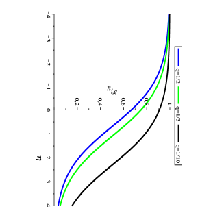
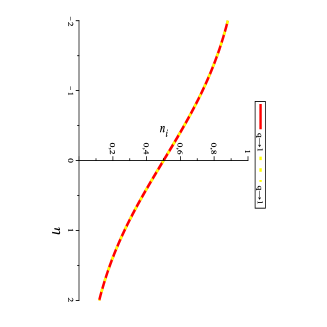
Figure 1: $n_{i}^{(q)}$ (left) and $n_{i,q}$ (center) as a function of $\eta=\beta(\epsilon_{i}-\mu)$ and overlap of $n_{i}^{(q)}$ with $n_{i,q}$ (right) as $q\to 1$.

In the sequence we will apply the two cases of deformation given by the Eqs.(12), (23) to the Landau diamagnetism problem, obtaining generalized thermodynamic quantities.

IV $q$-deformed Landau diamagnetism

To explain the phenomenon of diamagnetism, we have to take into account the interaction between the external magnetic field and the orbital motion of electrons. Disregarding the spin, the Hamiltonian of a particle of mass m and charge e in the presence of a magnetic field H is given by sal

$${\cal H}=\frac{1}{2m}\left({\bf p}-\frac{e}{c}{\bf A}\right)^{2},$$ (24)

where A is the vector potential associated with the magnetic field H and c is the speed of light in CGS units.

IV.1 $q$-Fermions application

Let us start formalizing the statistical mechanical problem by using the logarithm of the grand partition function $\Xi^{(q)}$, given in the form

$$\ln\Xi^{(q)}=\frac{2eHL^{3}}{hc(2\pi)}\displaystyle\sum_{n}^{\infty}\displaystyle\int_{-\infty}^{\infty}k_{z}\left[\frac{1}{2|\ln(q)|}\left|\ln\left(\frac{|a|}{qb}\right)\ln\left(\frac{c}{b}\right)+{\rm Li}_{2}\left(\frac{|a|}{qb}\right)+{\rm Li}_{2}\left(\frac{c}{b}\right)\right|\right],$$ (25)

where $a=\exp(\beta\epsilon_{n})-z$, $b=\exp(\beta\epsilon_{n})+zq$, $c=\exp(\beta\epsilon_{n})(q^{2}+1)$, $k_{z}=-\infty,\cdots,\infty$, $\epsilon_{n}=\frac{\hbar^{2}k_{z}^{2}}{2m}+\hbar\omega\left(n+\frac{1}{2}\right)$, $\omega=\frac{eH}{mc}$ and ${\rm Li}_{2}$ is dilogarithm function,

$${\rm Li}_{2}(x)=-\displaystyle\int_{0}^{x}dt{\frac{\ln(t)}{1-t}}.$$ (26)

As we know the Landau diamagnetism problem is solved in the limit of high temperatures $(z\ll 1)$. Thus, we will carry it out a Taylor expansion until second order of Eq.(25), which allows us the analysis of the insertion of the $q$-deformation. After performing some calculations we obtain

$$\ln\Xi^{(q)}=\frac{zHC}{\sinh(\gamma)}Q_{1}-\frac{z^{2}HC\sqrt{2}}{8\sinh(2\gamma)}Q_{2},\qquad\mbox{where}\qquad C=\frac{eL^{3}}{hc\lambda_{T}},$$ (27)

$$Q_{1}=\left|\frac{q-q^{-1}}{2\ln(q)}\right|,\qquad Q_{2}=\left|\frac{q^{2}-q^{-2}}{4\ln(q)}\right|,$$ (28)

$\lambda_{T}={h}/\sqrt{2\pi m\kappa_{B}T}$ is the thermal wavelength, $\gamma=\beta\mu_{B}H$ and $\mu_{B}=\frac{e\hbar}{2mc}$ is Bohr magneton. In the sequence we have the $q$-deformed thermodynamic quantities. We first obtain the number of particles $N$ and the internal energy $U$ by the following equations

$$N^{(q)}=z\frac{\partial}{\partial z}\ln{\Xi^{(q)}}=\frac{zHC}{\sinh(\gamma)}Q_{1}-\frac{z^{2}HC\sqrt{2}}{4\sinh(2\gamma)}Q_{2}.$$ (29)

and

$$U^{(q)}=-\frac{\partial}{\partial\beta}\ln\Xi^{(q)}=\frac{zC\mu_{B}H^{2}\coth(\gamma)}{\sinh(\gamma)}Q_{1}-\frac{z^{2}C\mu_{B}H^{2}\sqrt{2}\coth(2\gamma)}{4\sinh(2\gamma)}Q_{2}.$$ (30)

The grand potential $\phi^{(q)}$ is obtained as

$$\phi^{(q)}=-\frac{1}{\beta}\ln\Xi^{(q)}=-\left[\frac{zHC}{\beta\sinh(\gamma)}Q_{1}-\frac{z^{2}HC\sqrt{2}}{8\beta\sinh(2\gamma)}Q_{2}\right],$$ (31)

from which we can determine the entropy

$$S^{(q)}=-\frac{\partial\phi^{(q)}}{\partial T}=\kappa_{B}\left\{\frac{zHC(1+\gamma\coth(\gamma))}{\sinh(\gamma)}Q_{1}-\frac{z^{2}HC\sqrt{2}(1+2\gamma\coth(2\gamma))}{8\sinh(2\gamma)}Q_{2}\right\}.$$ (32)

Also, applying the definition of the Langevin function we write

$${\cal L}(\gamma)=\coth(\gamma)-\frac{1}{\gamma},\qquad{\cal L}(2\gamma)=\coth(2\gamma)-\frac{1}{2\gamma}.$$ (33)

Now deriving the Eq.(31) with respect to the magnetic field, using $N^{(q)}$ to eliminate the chemical potential and inserting the Langevin functions in Eq.(33) we obtain the magnetization

$$M^{(q)}=-\frac{\partial\phi^{(q)}}{\partial H}=-N^{(q)}\mu_{B}\left\{\frac{z\sqrt{2}\sinh(\gamma)(q^{2}+1){\cal L}(2\gamma)-8|q|\sinh(2\gamma){\cal L}(\gamma)}{z\sqrt{2}\sinh(\gamma)(q^{2}+1)-8|q|\sinh(2\gamma)}\right\}.$$ (34)

IV.2 $F$-Anyons application

Now starting with Eq.(23), we write the logarithm of the grand partition function $\Xi_{q}$. The procedures performed in the sequence will be the same as for the $q$-fermions case. Therefore,

$$\ln\Xi_{q}=\frac{2eHL^{3}}{hc(2\pi)}\displaystyle\sum_{n}^{\infty}\displaystyle\int_{-\infty}^{\infty}k_{z}\ln[1+zq^{-1}\exp(-\beta\epsilon_{n})],$$ (35)

that by considering the limit of high temperatures $(z\ll 1)$ we find

$$\ln\Xi_{q}=\frac{zHC}{q\sinh(\gamma)}-\frac{z^{2}HC\sqrt{2}}{8q^{2}\sinh(2\gamma)},\qquad\mbox{where}\qquad C=\frac{eL^{3}}{hc\lambda_{T}},$$ (36)

from which, we get in the sequence the number of particles

$$N_{q}=z\frac{\partial}{\partial z}\ln{\Xi_{q}}=\frac{zHC}{q\sinh(\gamma)}-\frac{z^{2}HC\sqrt{2}}{4q^{2}\sinh(2\gamma)},$$ (37)

the internal energy

$$U_{q}=-\frac{\partial}{\partial\beta}\ln\Xi_{q}=\frac{zC\mu_{B}H^{2}\coth(\gamma)}{q\sinh(\gamma)}-\frac{z^{2}C\mu_{B}H^{2}\sqrt{2}\coth(2\gamma)}{4q^{2}\sinh(2\gamma)},$$ (38)

and the grand potential

$$\phi_{q}=-\frac{1}{\beta}\ln\Xi_{q}=-\left[\frac{zHC}{q\beta\sinh(\gamma)}-\frac{z^{2}HC\sqrt{2}}{4q^{2}\beta\sinh(2\gamma)}\right].$$ (39)

Now with Eq.(39) we can also determine the entropy

$$S_{q}=-\frac{\partial\phi_{q}}{\partial T}=\kappa_{B}\left\{\frac{zHC(1+\gamma\coth(\gamma))}{q\sinh(\gamma)}-\frac{z^{2}HC\sqrt{2}(1+2\gamma\coth(2\gamma))}{8q^{2}\sinh(2\gamma)}\right\}.$$ (40)

As in the previous section, by deriving the Eq.(39) with respect to the magnetic field, using $N_{q}$ to eliminate the chemical potential and inserting the Langevin functions in Eq.(33) we obtain the magnetization

$$M_{q}=-\frac{\partial\phi_{q}}{\partial H}=N_{q}\mu_{B}\left\{\frac{z\sqrt{2}\sinh(\gamma)(q^{2}+1){\cal L}(2\gamma)-4q\sinh(2\gamma){\cal L}(\gamma)}{z\sqrt{2}\sinh(\gamma)-4q\sinh(2\gamma)}\right\}.$$ (41)

The Figs. 2 and 3 show that the magnetization curves are dependent on the values of the parameter $q$. Noticed that even with the same values for the two cases of $q$-deformation, the behaviors are quite different. However, it is worth noting that for the case that we have the limit $q\to 1$ the behaviors are identical, as expected.

We can also observe that as the value of $q$ approaches zero (greater insertion of the $q$-deformation) the behaviors of the curves are similar in both cases. The black curves call attention for the distinct behaviors in the range $0-2Oe$ of the magnetic field, and above this value follow the other curves in a similar fashion. Another important fact, with respect to these curves ($q=0.1$), is that for F-anyons statistics the magnetization, Fig. 3 (center), shows a more strong response with respect to magnetic field in relation to the magnetization for $q$-fermions statistics in the same range of field. This fact may be used to verify such behavior experimentally, for instance, in superconductors which are perfect diamagnetic materials and have strong magnetic susceptibility, by inserting impurities, or changes in pressure or temperature.

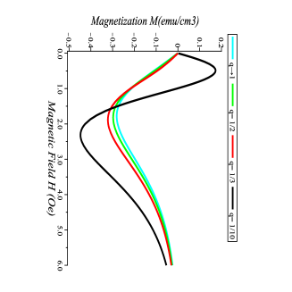
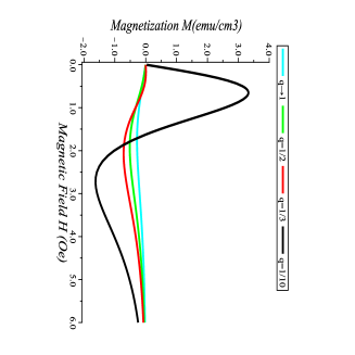
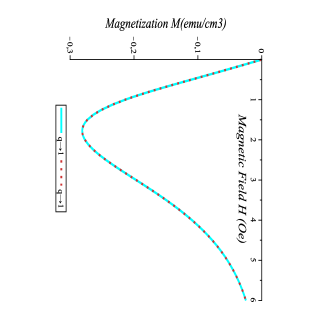
Figure 2: $q$-deformed magnetization as a function of magnetic field H for several choices of $q$. $M^{(q)}$ (left), $M_{q}$ (center) and overlap of $M^{(q)}$ with $M_{q}$ (right).

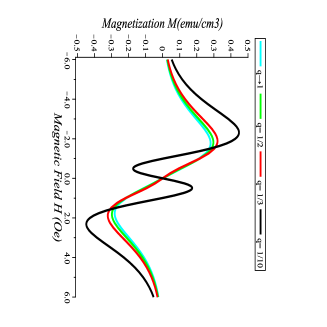
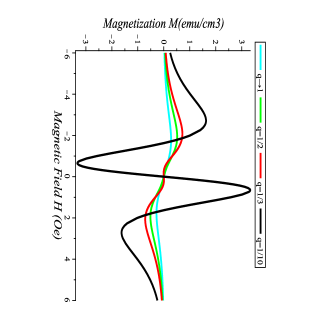
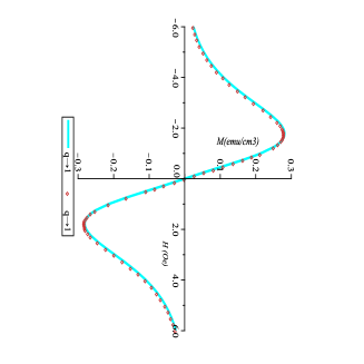
Figure 3: $q$-deformed magnetization as a function of magnetic field H for several choices of $q$. $M^{(q)}$ (left), $M_{q}$ (center) and overlap of $M^{(q)}$ with $M_{q}$ (right).

V Conclusions

We investigate generalized fermions through two $q$-deformed models: $q$-fermions and F-anyons. An interesting fact is that the Pauli exclusion principle is still valid for F-anyons, whereas for the $q$-fermions model it has to be enforced by hand, explicitly or implicitly nar .

Other observations with respect to the $q$-fermions and F-anyons are in order. As in the former case, we have the definition of the basic number we could have made the derivatives through the Jackson derivatives (JD), such as bri1 ; bri2 ; Marinho:2018gce . We did not decide for such an application, because when obtaining $q$-deformed grand partition function for high temperature, we can perform calculations with ordinary derivatives to obtain the same results as those from JD. On the other hand, the F-anyons only allow the application of the usual derivatives, because, as we have seen, their algebra does not have a defined basic number. Thus, the application of ordinary derivatives is applied straightforwardly to obtain thermodynamic quantities. Further related issues can be addressed in more general algebras such as hybrid algebras Marinho:2019zny .

Finally, regardless of the model, we have seen that the parameter $q$ modifies the statistics, and that in the limit $q\to 1$ we have the standard fermionic statistics, as expected. Of course, the fact that the Landau diamagnetism problem is solved in the limit of high temperatures at first order, causes the models to be very well tractable. However, differently from what we find in the literature sal we have expanded the problem up to second order to get better expressions that explicitly show the effect of the deformed statistics. An important observed fact is that for F-anyons statistics the magnetization, Fig. 3 (center), shows a more strong response with respect to magnetic field in relation to the magnetization for $q$-fermions statistics in the same range of field. The results reported here may be verified experimentally, for instance, in superconductors by inserting impurities, or changes in pressure or temperature if one assumes these tuning quantities are related with the $q$-deformation parameter.

References

- (1) J. M. Leinaas and J. Myrheim, Nuovo Cimento B 37, 1 (1977).
- (2) F. Wilczek, Fractional Statistics and Anyon Superconductivity, World Scientific, Singapore, (1990).
- (3) S.S. Chern, et al., Physics and Mathematics of Anyons, World Scientific, Singapore, (1991).
- (4) R. Iengo, K. Lechener, Phys. Reports 213, 179-269 (1992).
- (5) A. Lerda and S. Sciuto, Nucl. Phys. B 401, 613 (1993).
- (6) J. Fuchs, Affine Lie Algebras and Quantum Groups, Cambridge University Press (1992).
- (7) L.C. Biedenharn, M.A. Lohe, Quantum Group Symmetry and -Tensor Algebras, World Scientific, Singapore, (1995).
- (8) A. Macfarlane, J. Phys. A: Math. Gen. 22, 4581 (1989).
- (9) R. Pharthasarathy, K.S. Viswanathan, J. Phys. A: Math. Gen. 24, 613-617 (1991).
- (10) M. Chaichian, R. Gonzales Felipe, C. Montonen, J. Phys. A: Math. Gen. 26, 4017 (1993).
- (11) L.P. Colatto, J.L. Matheus-Valle, J. Math. Phys. 37, 6121 (1996).
- (12) J. de Souza, E.M.F. Curado, M.A.R. Monteiro, J. Phys. A: Math. Gen. 39, 10415-10425 (2006).
- (13) G. Gervino, A. Lavagno, D. Pigato, J. Phys. Conf. Series 306, 012070 (2011).
- (14) M. Arik, D.D.Coon, J. Math. Phys. 17, 524 (1976).
- (15) M. Jimbo, Lett. Math. Phys. 10, 63-69 (1985).
- (16) D. Arovas, R. Schrieffer, F. Wilczek, and A. Zee, Nucl. Phys. B 251, 117 (1985).
- (17) D. Sen, Nucl. Phys. B 360, 397-408 (1991).
- (18) R. Acharya and P. Narayana Swamy, J. Phys. A 27, 7247 (1994).
- (19) R. Acharya and P. Narayana Swamy, J. Phys. A 37, 2527 (2004).
- (20) W. A. Perkins, Int. J. Theor. Phys. 41, 823 (2002).
- (21) A. Lavagno, P.N. Swamy, Physica A 389, 993-1001 (2010);
- (22) A. Rovenchak, Eur. Phys. J. B 87, 175 (2014).
- (23) A. Algin, D. Irk and G. Topcu, Phys. Rev. E. 91, 062131 (2015).
- (24) A. Algin, A.S. Arikan, E. Dil, Physica A 416, 499-517 (2014).
- (25) A. Algin, M. Senay, Phys. Rev. E. 85, 041123 (2012).
- (26) A. Algin, M. Senay, Physica A 447, 232-246 (2016).
- (27) P. N. Swamy, Int. J. Mod. Phys. B 20, 697-713 (2006).
- (28) G. Gentile, Nuovo Cimento 17, 493 (1940).
- (29) H. S. Green, Phys. Rev. 90, 270 (1953).
- (30) A. P. Polychronakos, Phys. Lett. B 365, 202 (1996).
- (31) C. Tsallis, J. Stat. Phys. 52, 479 (1988).
- (32) F. D. M. Haldane, Phys. Rev. Lett. 67, 937 (1991)
- (33) L. Landau, Z. Phys. 64, 629 (1930).
- (34) S.F.Özeren, et al, Eur. Phys. J.B. 2, 101-106 (1998).
- (35) Ö.F. Dayi., A. Jellal, Phys. Lett. A 287, 349-355 (2001).
- (36) A. Algin, M. Arik and A.S. Arikan, Phys. Rev. E. 65, 026140 (2002).
- (37) A. Algin, M. Senay, Phys. Rev. E 85, 041123 (2012).
- (38) A. Algin, Int. J. Theor. Phys. 50, 1554-1568 (2011).
- (39) P. N. Swamy, Int. J. Mod. Phys. B 20, 2537-2550 (2006).
- (40) P. N. Swamy, Eur. Phys. J. B 50, 291 (2006).
- (41) P. N. Swamy, Mod. Phys. Lett. B 15, 915-920 (2001).
- (42) K. S. Viswanathan, R. Parthasarathy, and R. Jagannathan, J. Phys. A 25, L335 (1992).
- (43) A. Lavagno, N.P. Swamy, Phys. Rev. E 65, 036101 (2002).
- (44) T. Ernst, The History of -calculus and a new method. (Dep. Math., Uppsala Univ. 1999-2000).
- (45) E.G. Floratos, J. Phys. Math. 24, 4739 (1991).
- (46) H. Exton, -Hypergeometric Functions and Applications, John Wiley and Sons, New York, (1983).
- (47) A.M. Scarfone, P.N. Swamy, J. Stat. Mech. Theor. Exp. P02055, 02 (2009).
- (48) A.M. Gavrilik, A.P. Rebesh, Mod. Phys. Lett. B 25, 1150030 (2012).
- (49) S.R.A. Salinas, Introdution to Statistical Physics, Springer-Verlag, NY (2001)
- (50) F.A. Brito, A.A. Marinho, Physica A 390, 2497-2503 (2011).
- (51) A.A. Marinho, F.A. Brito, C. Chesman, Physica A 411, 74-79 (2014).
- (52) A. A. Marinho and F. A. Brito, J. Math. Phys. 60, no. 1, 012101 (2019) doi:10.1063/1.5040016 [arXiv:1805.03229 [cond-mat.stat-mech]].
- (53) A. A. Marinho and F. A. Brito, arXiv:1904.07843 [cond-mat.stat-mech].