Sparse Matrix to Matrix Multiplication: A Representation and Architecture for Acceleration

Abstract

Accelerators for sparse matrix multiplication are important components in emerging systems. In this paper, we study the main challenges of accelerating Sparse Matrix Multiplication (SpMM). For the situations that data is not stored in the desired order (row/column order), we propose a compact high performance sparse format, which allows for random access to a dataset with low memory access overhead. We show that using this format results in a 14-49 times speedup for SpMM. Next, we propose a high performance systolic architecture for SpMM, which uses a mesh of comparators to locate the useful (non-zero) computation. This design maximizes data reuse by sharing the input data among a row/column of the mesh. We also show that, with similar memory access assumptions, the proposed architecture results in a 9-30 times speedup in comparison with the state of the art.

I Introduction

In emerging data-inference applications the data-set is often large and sparse. Hardware accelerators can benefit from sparse formats for these datasets as those store only the non-zero elements, reducing the required storage and bandwidth. A common kernel in this context is sparse matrix multiplication (SpMM). This is used in many applications such as graph analysis, including breadth first search [8] and graph clustering [18], in addition to its scientific applications in algebraic multi-grid solving [3] and quantum modeling [17]. While there are many accelerators suggested in the literature for sparse matrix to vector (SpMV) multiplication [13, 10, 7], there are only a few proposed accelerators for SpMM. Accelerating SpMM cannot always be simplified to SpMV acceleration. As the second operand of SpMM is a two dimensional matrix rather than a vector. This poses additional challenges:

Accessing data in two different orders: In SpMM, the first dataset (the multiplicand) is accessed in row order and the other (the multiplier) is accessed in column order. However, sparse data formats store the non-zeros in one order, say row-order. Accessing data in the other orders has a high cost in the number of memory accesses (MA) and it might not be practical to store the large datasets in both orders. For instance, suppose matrix $A$ is stored in row order and appears as the first operand in $A\times B$. In another matrix multiplication, the same matrix $A$ might appear as the second operand, where it needs to be stored in column order.

Complexity of the SpMM algorithm: Designing a high performance SpMM algorithm is challenging. SpMM algorithms should skip operations on zero elements. However, in unstructured sparse datasets, location of zeros is arbitrary. This makes it non-trivial to locate the non-zeros without incurring an overhead that overwhelms the benefit of skipping zeros. This challenge will be elaborated in Section II.

The first challenge, which is a special case of accessing sparse data in non-trivial patterns, has not been studied in the literature thus far. There are various high performance sparse formats proposed in the literature [12, 16, 4, 7]. However, most of these are proposed for SpMV acceleration, and therefore, they do not address the non-trivial access challenge. On the architecture front, to the best of our knowledge, there is only one work to design a systolic-like structure for SpMM, the FPIC design [11]. In a conventional matrix multiplier (MM), there is a mesh of multiplier and accumulator (MAC) nodes and input data is shared among a row or a column of those nodes. This maximizes the reusability of data.

The previous FPIC SpMM design [11] does not have data sharing along the rows and columns, and each MAC node reads all its arguments directly from the inputs. To reduce memory bandwidth, these inputs are buffered at the rows and columns. This buffering limits the size of the SpMM unit and the lack of scalability increases the overall latency when it targets large matrices.

In addressing the above gaps, this paper makes the following contributions: (i) We propose the Indexed Compressed Row Storage (InCRS) format, a new row-based sparse format with reduced memory access for arbitrary access patterns. We show how using InCRS can speedup SpMM when the dataset is not stored in the desired order. (ii) We propose a high performance and scalable systolic SpMM. In the proposed architecture, input is shared among a row or a column of the nodes and allows for maximum data reuse.

We evaluate our design on a range of large and sparse datasets. Using InCRS format when the second dataset is not stored in row-order, can speedup SpMM $\approx$ 14-49 times. Further, our systolic SpMM can speedup matrix multiplication 9-30 times in comparison with the state of the art FPIC design.

II Complexity of Non-Trivial Data Access in Sparse Formats

In matrix multiplication the first matrix is accessed in row order and the second in column order. Since the second matrix might be accessed in row order in another application, e.g., being the first operand of another matrix multiplication, we assume all matrices are stored in one order, which we assume is row order (assuming column order is fine too, and will just switch the direction of our solution). Sparse formats store the non-zeros in one order, say row order, and accessing data in other orders is complex. For instance, to read one column of data stored in a row-based format, many of the non-zeros of each row are accessed to locate the elements of that column. In the following, we briefly study popular unstructured sparse formats and their cost of random data access.

II-A Popular Unstructured Sparse Formats

1. ELLPACK: One matrix stores the non-zero values of row $i$ in its $i^{th}$ row and another matrix stores the column indices of the non-zeroes [14].

2. List of lists (LiL): A vector stores pointers to the beginning of each row. Then the non-zeros of each row are stored in a separate linked list.

3. Co-ordinate list (COO) and 4) Single linear list (SLL): The non-zero values and their row and column indices are stored sequentially.

4. Jagged diagonal (JAD): JAD is not row or a column order. It first sorts the rows of the matrix in descending order based on their number of non-zeros. Then it stores the non-zero values and their column indices starting with the first non-zeros of all the rows, then the second non-zeros of the rows and so on. One vector ($jadPtr$) stores pointers to the non-zeros of the first row [6].

5. Compressed row storage (CRS): CRS stores the non-zero values and their column indices in two vectors. Another vector provides pointers to the first non-zero of each row. Compressed column storage (CCS) is the transpose of CRS, where the matrix is stored in column order.

II-B Cost of Non-Trivial Data Access

Table I compares the complexity of reading one arbitrary element in sparse formats, where $M$ and $N$ are the number of rows and columns. $D$ is the density, i.e., the ratio of the number of non-zeros to the dataset size. Note that in conventional dense format, a single memory access is enough to read an arbitrary element.

TABLE I: Complexity of locating one data in sparse formats.

Formats	MA complexity	Avg # of MA
ELLPACK,	Access all the NZa before the	$\frac{1}{2}.N.D$
LiL,CRS	desired element in each row.
JAD	Search through the NZs of a row, one by	$N.D$
	one. Unlike in CRS, the NZs of a row
	are not stored sequentially. Thus, locate
	each one of them using $jadPtr$.
COO,	There is no pointer. Access all the	$\frac{1}{2}.M.N.D$
SLL	NZs located before the desired element.

As Table I shows, CRS has amongst the least memory access requirements while it is also amongst the most compact formats. Further, previous work [9] has shown that CRS incurs the lowest number of memory accesses in many linear algebra operations. However, CRS still incurs a high number of memory accesses in comparison with the conventional dense format. Next, we propose a low-overhead improvement for accessing arbitrary data in CRS.

III Accelerating Non-Trivial Data Access in Sparse Formats

Suppose matrix $B$ is the second operand in an SpMM operation, then, SpMM needs to access elements of the columns of $B$ in order. To read element $B[i][j]$ in CRS format, first the beginning of row $i$ is located, then all non-zero elements in that row ($B[i][:]$) and before column $j$ are accessed until $B[i][j]$ is located. This incurs an average of $\approx\frac{1}{2}.N.D$ memory accesses, which could be large for large datasets. For instance, for the Docword dataset from the NIPS 2013 challenge [15] with 12k columns and 4% density, on average 240 memory accesses are required to locate one arbitrary element. This makes reading a matrix in column order too slow.

We propose to augment CRS by storing some information about the non-zeros in each row. Suppose we want to locate element $B[i][j]$. If we knew how many non-zeros exist before $B[i][j]$ in row $i$, say $n_{i,j}$ elements, then we could start from the beginning of the row $i$ and skip $n_{i,j}$ elements to locate $B[i][j]$ at the $(n_{i,j}+1)^{th}$ location in the row. We propose the Indexed CRS (InCRS) format, which augments the CRS format with such information.

III-A Indexed CRS (InCRS) Format

InCRS divides each row into sections of $S$ elements, which are sub-divided into blocks of $b$ elements. It stores information on the number of non-zeros inside the sections and blocks. To access $B[i][j]$, this information is used to find the number of non-zeros that exist before the respective block to locate that block. This information is represented using counter-vectors, which are the addition to CRS. Each counter-vector is designed to be single word and stores information of one section. Therefore, to access the counter-vector of a section, only one memory access is required.

Figure 1 shows an example of a row with 24 columns. In this setup, the row is divided to sections of 8 elements ($S=8$) and each section is divided to blocks of 2 elements ($b=2$). The first part of the counter-vector stores the total number of non-zeros that exist in the previous sections of that row and the rest of it stores information about the number of non-zeros inside each block in that section. In this example, the counter-vector indicates that there are between 5 to 7 number of non-zeros(NZs) located in row $i$ and before column $j=13$.

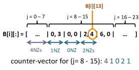
Figure 1: Example of a counter-vector for a section of a row.

To locate $B[i][j]$, we first locate its counter-vector. $B[i][j]$ belongs to the section number $\lfloor{\frac{j}{S}\rfloor}$ and block number $\lfloor\frac{j\%S}{b}\rfloor$, where $\lfloor\frac{x}{y}\rfloor$ represents integer quotient of dividing $x$ by $y$, and $x\%y$ is the remainder of this division. Using the counter-vector, we find the number of non-zeros located before the $B[i][j]$’s block. For this, we add the number of non-zeros that exist before $B[i][j]$’s section (first part of the counter-vector) to the number of the non-zeros that exist in the blocks inside this section but before $B[i][j]$’s block. We then use this offset from the beginning of row $i$ to locate $B[i][j]$’s block and search through the elements of that block to locate $B[i][j]$. This means we can limit our search for the element $B[i][j]$ to only its block, which requires an average of $\approx\frac{b}{2}$ memory accesses. Recall that the counter-vector of each section is a single word and requires only one memory access. Therefore the average of overall memory accesses to locate a random element in this format is $\approx\frac{b}{2}+1$.

III-B Implementation of InCRS

In our implementation, the section size is 256 elements ($S=256$) and the blocks are 32 elements ($b=32$). In this implementation each counter-vector has 64 bits, where 8 $\times$ 6 bits are used for storing the non-zeros inside the 8 blocks. The remaining 16 bits of the counter-vector store the number of non-zeros before this section. This is based on the assumption that each row has maximum of 65k non-zeros, which is reasonable for a sparse dataset. Note that these parameters can be adjusted for a given dataset.

III-C Accelerating SpMM Data Access

As mentioned before, the CRS format requires on average $\approx\frac{1}{2}.N.D$ accesses to locate $B[i][j]$ and InCRS reduces this to around $\frac{b}{2}+1$, which means the memory access reduces by a factor of $\frac{N.D}{b+2}$. This is the estimated reduction factor of memory accesses for reading one column of the dataset. Table II shows this estimated factor for the 5 large and sparse datasets that we used in our experiments. The datasets are further discussed in Section V. The memory access ratio indicates that the datasets with a larger number of non-zeros in each row benefit more from using InCRS.

TABLE II: Cost and benefit of InCRS compared to CRS.

Dataset	Dimension	$D$	NZs per row	MA	Storage
	($M\times N$)		(min, avg, max)	ratio	ratio
Amazon	300 $\times$10k	14%	(501, 1400, 2011)	42	0.99
Belcastro	370 $\times$ 22k	6%	(1, 1300, 6787)	39	0.97
Docword	700 $\times$ 12k	4%	(2, 480, 906)	14	0.95
Norris	1200 $\times$ 3.6k	1%	(3, 360, 795)	11	0.98
Mks	3.5k $\times$ 7.5k	1.5%	(18, 150, 957)	3	0.88

The main cost of this improvement is the additional storage required for the counter-vectors. In our design, we require a 64bit counter-vector for each section (256 elements) of a row. Thus, this extra storage is $\frac{1}{S}.N.M$ words. Since the storage required for CRS is $\approx 2.M.N.D$ words, the ratio of the storage required for CRS format to the storage for InCRS format is $\approx\frac{2D.S}{2D.S+1}$, which we refer to as storage ratio in Table II. As the Table shows, for these datasets, the storage required for CRS varies between 0.99 and 0.88 of the storage required to store the same datasets in InCRS format. It is clear that by reducing the size of the blocks the storage overhead (small $b$ is needed to fit the counter-vector in a word) and the expected benefit both increase.

IV Systolic SpMM Architecture

In the previous section we proposed using the InCRS format to accelerate accessing the matrix elements for SpMM. In this section, we assume that data can be accessed fast enough and we focus on the SpMM architecture.

IV-A Main Challenges of Implementing SpMM

Figure 2a depicts a $3\times 3$ conventional systolic matrix multiplier, which we refer to as conventional MM.

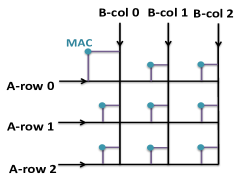
(a) Conventional systolic MM.

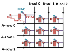
(b) The proposed systolic SpMM.

Figure 2: $3\times 3$ systolic matrix multiplier.

Each node in this mesh consumes two operands per cycle, either zero or non-zero, and performs a multiply-accumulate (MAC) on the pair. This gets more complicated in an SpMM architecture, since the nodes receive the data in sparse format. Each node in the SpMM case receives two sparse vectors (row of $A$ and column of $B$ in $A\times B$) and compares the indices, before MAC operations. Algorithm 1 describes one cycle of the sparse dot product algorithm that each node of the mesh performs. Here, $c$ is the final product of the node. Vectors $a_{index}$ and $a_{val}$ hold the indices and values of nonzero elements in vector $a$, a row of matrix $A$. Similarly, vectors $b_{index}$ and $b_{val}$ hold the indices and values for vector $b$, a column of matrix $B$.

Algorithm 1 One cycle of index-matching and MAC operation at SpMM mesh nodes.

if ($a_{index}[i]$ = $b_{index}[j]$) then

    $c\leftarrow c+a_{val}[i]\times b_{val}[j]$

    $i\leftarrow i+1$

    $j\leftarrow j+1$

else if ($a_{index}[i]>b_{index}[j]$) then

    $j\leftarrow j+1$

else

    $i\leftarrow i+1$

end if

In this comparison, if the indices are equal, MAC is performed on the operands and both counters $i$ and $j$ are incremented. When the counter of an operand is incremented, that operand is consumed and a new data can be read from the input. When the indices do not match, only the operand with smaller index is consumed while the operand with larger index is kept, i.e., either counter $i$ or $j$ is incremented. This asymmetric operand consumption results in a slower movement of operands than in conventional MM. Moreover, it results in stalling when the inputs are shared, i.e. the input is passed along multiple nodes along a row/column of the mesh.

FPIC is the state of the art $8\times 8$ systolic-like architecture proposed in [11]. In that work, because of the discussed complexity in sharing the operands along a row/column, each node of the systolic architecture reads and compares the operands independently. This results in a high bandwidth requirement to memory, which is avoided in the FPIC design by buffering the input data. In this design, each node of the mesh reads from 8 possible buffers along the row, and from 8 possible buffers along the column, i.e. $8\times 8=64$ buffers are used for reading data from matrix $A$ and 64 buffers to read data from matrix $B$. Each of these buffers is 32-element wide.

The main disadvantage of this design is that this buffering method limits the mesh size. In this work, they fixed the mesh size to $8\times 8$ and to scale the design, they suggest to use multiple $8\times 8$ units. In the following, we propose a synchronized mesh of comparators that overcomes the above-mentioned challenges.

IV-B Proposed Synchronized Mesh

As mentioned above, the main advantages of the conventional systolic MM are: i) fast operand consumption, ii) sharing operands among a row or a column of nodes maximizing data reuse. We achieve this by a synchronized movement of the input data through the mesh of the comparators (Figure 2b). Each node of this mesh has a comparator, a buffer of operands and a flag, which are located before the MAC unit.

Comparison process of the nodes

Algorithm 2 One cycle of index-matching and MAC operation at each node of the proposed synchronized mesh.

1:if ($a_{index}[i]$ = $b_{index}[j]$) then

2:    $c\leftarrow c+a_{val}[i]\times b_{val}[j]$

3:    $reset(buffer_{op},flag_{op})$

4:else if ($a_{index}[i]>b_{index}[j]$) then

5:    if ($flag_{op}$= $A$) then

6:         $(matched,val)\leftarrow search(b_{index}[j],buffer_{op})$

7:         if ($matched$) then

8:             $c\leftarrow c+val\times b_{val}[j]$

9:         end if

10:    else

11:         reset $buffer_{op}$

12:         $flag_{op}\leftarrow A$

13:    end if

14:    $buffer_{op}\leftarrow[a_{index[i]},a_{val[i]}]$

15:else

16:    if ($flag_{op}$= $B$) then

17:         $(matched,val)\leftarrow search(a_{index}[i],buffer_{op})$

18:         if ($matched$) then

19:             $c\leftarrow c+val\times a_{val}[i]$

20:         end if

21:    else

22:         reset $buffer_{op}$

23:         $flag_{op}\leftarrow B$

24:    end if

25:    $buffer_{op}\leftarrow[b_{index[j]},b_{val[j]}]$

26:end if

27:$i\leftarrow i+1$

28:$j\leftarrow j+1$

As algorithm 2 describes, at each node, the comparator reads in two new operands, one along the row and one along the column, and compares their indices. If they match, the MAC operation is performed on them. If they do not match, it buffers the operand with the larger index (lines 14 and 25) and sets the $flag_{op}$ to indicate which operand ($A$ or $B$) has been buffered. The use of operand buffers allows for keeping the data moving and prevent stalling. Also, it allows for always consuming two operands (lines 27 and 28) rather than one or two operands per cycle at each node. This is possible since in the cases that operands’ indices do not match, the operand with larger index is buffered instead of stalling, thus its counter still increments. Note that the buffer is not always occupied. It is flushed in some cases, e.g., when the indices of the operands match.

When the indices of the new operands do not match, the $flag_{op}$ is checked. If the operand with the smaller index can be matched with an operand residing inside the buffer, which is determined by checking the $flag_{op}$ at lines 5 and 16, the $buffer_{op}$ is searched. Here, $search(x,buffer)$ means searching $x$ among the operand indices stored in the $buffer$. The Boolean variable $matched$, indicates if the match was successful, and $val$, the value of the matched operand. Since the operand indices are sorted, $search$ operation requires at most $log_{2}(Depth_{buffer})$ comparisons. Considering small size of the buffers (32 elements here), we can use content addressable memories (CAM) to further accelerate $search$.

Synchronization

To prevent stalling, reading the rows and columns is synchronized at the end of each round of $R$ elements. This means that, at the $k^{th}$ round, each row or column accesses operands with indices between $k\times R$ and $(k+1)\times R$, then they wait for the rest of the rows and columns to finish the round. On starting a new round all the operand buffers are reset since any remaining buffer operands are no longer needed. This way, the operand buffers need to be at most $R$-element in size ($Depth_{op}=R$) to prevent any stall. In this work, we set $R$ to 32 elements. However, there is a trade off as larger $R$ allows for faster movement of the data because of less synchronization, at the cost of larger buffer overhead and search of the buffer elements.

Overall, the main advantages of this architecture are maximizing the data reuse and fast consumption of the operands. It also has a simple data access, avoiding extra buffering at the input ports, which makes the design scalable. The main drawbacks are the extra buffering and the search process through the buffer elements at each node. In the following, we evaluate this design and compare it with FPIC and conventional MM.

V Experiments

We evaluated acceleration of SpMM memory access when using the InCRS format. Then, we evaluated the proposed systolic SpMM architecture.

V-A Methodology

In the first set of experiments, our goal is to evaluate memory access acceleration when using the InCRS format for SpMM operation. For this, we used the Gem5 [2] tool, which allows for simulating the memory hierarchy. Table III summarizes the simulation parameters, which contains the typical values of memory size and other parameters.

TABLE III: Gem5 simulation parameters.

CPU	Single core @ 1GHz frequency
L1 Data Cache	32kB, 2-way associative, LRU, Block Size=64
L1 Instruction Cache	32kB, 2-way associative, LRU
Hit Latency	2
L2 Cache	1MB, 8-way associative, LRU, Block Size=64
Hit Latency	20
Prefetching	Stride prefetching with degree 4.

In the second set of the experiments, we assume memory access is fast enough and the required data is ready at each clock cycle. Here, we aim to evaluate the latency of the SpMM algorithms. For this, we used cycle accurate simulation to model the accelerator’s behavior.

V-B SpMM Memory Access Acceleration using InCRS

As mentioned in Section III-C, the gain from using the InCRS format depends on the number of non-zeros per row. Therefore, we have selected datasets with a different average number of non-zeros per row ranging from 150 to 1400 per row (Table II)[5, 15]. We select datasets such as graph and network applications, as well as bag of words and user ratings that are used by inference applications.

We resized our target datasets because of the slow simulation speed in the experiments. We simplified the first operand (in SpMM) to a vector since the focus of this work is the column-order memory access to the second operand. Also, simplifying this part of the computation is fair because row-order access to a matrix is the same for the CRS and the InCRS formats. To resize the second operand, we randomly removed a number of rows from the datasets. At the end, the resized datasets were larger than at-least twice the L2 size to avoid eliminating the possible L2 cache miss effects. Table II reports the sizes of the second operand after they are resized. We did not change or remove any of the columns of the second operand, since the columns’ lengths and distributions of non-zeros are important factors in this comparison.

Figure 3 summarizes the benefits of replacing CRS format by InCRS for SpMM.

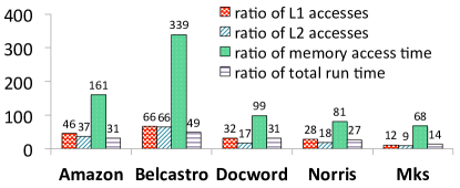
Figure 3: CRS vs. InCRS memory access ratio

This figure shows the number of cache accesses, total memory access time, and total run time when using CRS format normalized to the same parameters when using InCRS. As the figure shows, the number of cache accesses decrease for all the datasets with InCRS. The ratios of memory access reduction for different datasets are close to our estimations in Table II. For instance, the L1 access is decreased 49 and 31 times for Belcastro and Docword datasets, which is close to our estimation of 39 and 14 times reduction, respectively, in Table II. Here, the average cache miss latency was 11k-22k cycles for L1 and 75k-91k cycles for L2.

The third column in Figure 3 shows the ratio of the overall time spent on memory accesses. As a result of memory access speedup, the overall execution time of SpMM decreases noticeably for all the datasets. For instance, SpMM on Docword is around 31 times faster if we use InCRS instead of CRS.

V-C Evaluation of the Systolic SpMM Architecture

We compare the performance of our proposed architecture with the conventional MM and the FPIC work [11] performing $A\times A^{T}$ on a set of large and sparse datasets with a range of different densities (Table IV).

TABLE IV: Datasets used in the order of their densities.

Dataset	Amazon	Docword	Mks	Norris
$D$	14%	4%	1.5%	1%
Dimension	$1.5k\times 10k$	$1.5k\times 12k$	$7.5k\times 7.5k$	$3.6k\times 3.6k$
Dataset	Arenas	Bates	Gleich	Sch
$D$	0.85%	0.11%	0.095%	0.057%
Dimension	$1k\times 1k$	$2.5k\times 2.5k$	$2.6k\times 2.6k$	$3.6k\times 3.9k$

The FPIC unit size is fixed to $8\times 8$ in [11] and to scale this design, the authors suggest to use multiple units. Since they do not provide details about how to schedule the computation among the multiple units, we assume the best case scenario, which is perfect load balancing among the units. Based on that, to estimate the latency of the computation when using $k_{FPIC}$ numbers of the $8\times 8$ units, we performed the computation using a single unit and divided the latency of the computation by $k_{FPIC}$.

Our design is different from FPIC in terms of the required bandwidth and buffers. To perform a fair comparison, we fix each of those two parameters one at a time and sweep the other one. As the focus of the following experiments is memory access and index-matching of SpMM, for simplicity we assume a single cycle latency for all operations including MAC and comparisons. This is the same for the conventional MM, FPIC, and the proposed SpMM.

Similar input bandwidth: The left side of equation 1 is the required bandwidth for our proposed design with a mesh of $N_{synch}\times N_{synch}$ nodes. The right side is the bandwidth required by FPIC, where $k_{FPIC}$ is the number of $8\times 8$ units, and $W_{tot}$ is the matrix elements’ widths. Here, we assume the index width is 16 bits and value width is 32 bits.

$${2\times N_{synch}}\times W_{tot}=2\times 8\times k_{FPIC}\times W_{tot}$$ (1)

Similar buffer sizes: The left side of equation 2 indicates the number of 32-element buffers required for the proposed method and the right side indicates this number for FPIC.

$$N_{synch}^{2}=2\times 8^{2}\times k_{FPIC}\vspace{-6pt}$$ (2)

Figure 4a shows that assuming the same input bandwidth, the synchronized mesh performs SpMM 2.5-20 times faster than FPIC for the high density dataset and 4-58 times faster for the sparser dataset. The main disadvantage of this design in comparison with FPIC is its higher overall buffer size. However, Figure 4b shows that even with the same overall buffer size and, consequently, lower bandwidth usage, the synchronized mesh still performs SpMM faster than FPIC for both the low and the high density datasets.

In the last set of experiments, we fixed the parameters for our design: $N_{synch}$ is set to 64, resulting in 4096 MAC nodes, which is  60% of floating point DSP slices available on the new Xilinx FPGA (Virtex Ultra Scale XCVU9P [1]). The rest of the parameters are set accordingly (Table V). Here, we selected reasonable values for our parameters based on FPGA resources and we performed cycle-accurate simulation to evaluate the design. In the future, we will study the parameter selection process in more detail and implement the design on FPGA.

TABLE V: SpMM design parameters.

Designs	#Units, $N\times N$	BW	#MACs	Buffer
		(kb/cycles)		(kB)
This work	1, $64\times 64$	6	4096	768
FPIC-same BW	8, $8\times 8$	6	512	192
FPIC-same buffer	32, $8\times 8$	24	2048	768
Conv. MM	1, 96$\times$96	6	9216	-

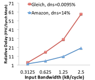
(a)

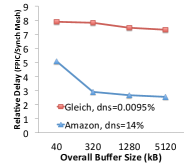
(b)

Figure 4: Comparison of the overall latency

Figure 5 compares the overall latency of the three designs for datasets with 0.057% to 14% density. Overall, our architecture’s acceleration increases as the density decreases. For this range of densities, the proposed architecture performs SpMM 1.5-39 times faster in comparison with the conventional MM and 2-30 times faster in comparison with FPIC. The lower performance of “FPIC-same-BW” design is a result of low DSP utilization and input BW (blue cell in Table V).

The red cells in Table V highlight the high resource requirement that might not be practical. For instance, the overall good performance of the conventional MM in these experiments is a result of large $N_{conv}$, which is set based on the $N_{conv}=\frac{W_{tot}}{W_{val}}\times N_{synch}$ equation assuming the same input BW for this design and the proposed SpMM. However, implementing this size of mesh is possible only if there are enough DSP resources available on the host FPGA.

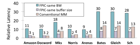
Figure 5: Latency of the different architectures normalized to the latency of the proposed synchronized mesh.

VI Conclusion

Matrix multiplication is a key kernel in inference applications, which often have large and sparse data sets. Thus, there is strong interest in accelerating this important operation with sparse data representations. We studied the main challenges of accelerating Sparse Matrix Multiplication (SpMM) including non-trivial data access and designing a systolic architecture. We proposed a modification to sparse formats to accelerate access to a dataset when the dataset is not stored in the desired order (row/column order). Our experiments show that the proposed InCRS format speeds up SpMM 14-49 times due to fewer memory accesses. Next, we proposed a high performance systolic SpMM architecture, which accelerates the computation and maximizes the data reuse by performing synchronized movement of the data through the architecture. We showed that, with similar memory access assumptions, the proposed architecture performs SpMM 9-30 times faster than the state of the art FPIC architecture.

References

- [1] UltraScale+ FPGAs, 2019. https://www.xilinx.com/support/documentation/ selection-guides/ultrascale-plus-fpga-product-selection-guide.pdf.
- [2] N. Binkert, B. Beckmann, G. Black, S. K. Reinhardt, A. Saidi, A. Basu, J. Hestness, D. R. Hower, T. Krishna, S. Sardashti, et al. The gem5 simulator. ACM SIGARCH Computer Architecture News, 39(2):1–7, 2011.
- [3] W. Briggs, V. Henson, and S. McCormick. A multigrid tutorial 2nd ed. Siam, Philadelphia, 2000.
- [4] A. Buluc, S. Williams, L. Oliker, and J. Demmel. Reduced-bandwidth multithreaded algorithms for sparse matrix-vector multiplication. In IPDPS. IEEE, 2011.
- [5] T. A. Davis and Y. Hu. The university of florida sparse matrix collection. TOMS, 38(1):1, 2011.
- [6] J. Dongarra, A. Lumsdaine, X. Niu, R. Pozo, and K. Remington. LAPACK working note 74: A sparse matrix library in C++ for high performance architectures. Technical report, University of Tennessee, 1994.
- [7] J. Fowers, K. Ovtcharov, K. Strauss, E. S. Chung, and G. Stitt. A high memory bandwidth fpga accelerator for sparse matrix-vector multiplication. In FCCM. IEEE, 2014.
- [8] J. R. Gilbert, S. Reinhardt, and V. B. Shah. A unified framework for numerical and combinatorial computing. Computing in Science & Engineering, 10(2), 2008.
- [9] P. A. Golnari and S. Malik. Evaluating matrix representations for error-tolerant computing. In DATE. IEEE, 2017.
- [10] S. Jain-Mendon and R. Sass. A case study of streaming storage format for sparse matrices. In ReConFig. IEEE, 2012.
- [11] E. Jamro, T. Pabiś, P. Russek, and K. Wiatr. The algorithms for fpga implementation of sparse matrices multiplication. Computing and Informatics, 33(3):667–684, 2015.
- [12] R. Kannan. Efficient sparse matrix multiple-vector multiplication using a bitmapped format. In HiPC. IEEE, 2013.
- [13] S. Kestur, J. D. Davis, and E. S. Chung. Towards a universal fpga matrix-vector multiplication architecture. In FCCM. IEEE, 2012.
- [14] D. R. Kincaid, T. C. Oppe, and D. M. Young. ITPACKV 2D user’s guide. Report CNA, UT Austin, 1989.
- [15] M. Lichman. UCI machine learning repository, 2013.
- [16] W. Liu and B. Vinter. Csr5: An efficient storage format for cross-platform sparse matrix-vector multiplication. In Proceedings of the 29th ACM on International Conference on Supercomputing. ACM, 2015.
- [17] E. H. Rubensson, E. Rudberg, and P. Sałek. Sparse matrix algebra for quantum modeling of large systems. In International Workshop on Applied Parallel Computing. Springer, 2006.
- [18] S. Van Dongen. Graph clustering via a discrete uncoupling process. SIAM Journal on Matrix Analysis and Applications, 30(1):121–141, 2008.