A hybrid particle volume-of-fluid method for curvature estimation in multiphase flows

Abstract

We present a particle method for estimating the curvature of interfaces in volume-of-fluid simulations of multiphase flows. The method is well suited for under-resolved interfaces, and it is shown to be more accurate than the parabolic fitting that is employed in such cases. The curvature is computed from the equilibrium positions of particles constrained to circular arcs and attracted to the interface. The proposed particle method is combined with the method of height functions at higher resolutions, and it is shown to outperform the current combinations of height functions and parabolic fitting. The algorithm is conceptually simple and straightforward to implement on new and existing software frameworks for multiphase flow simulations thus enhancing their capabilities in challenging flow problems. We evaluate the proposed hybrid method on a number of two- and three-dimensional benchmark flow problems and illustrate its capabilities on simulations of flows involving bubble coalescence and turbulent multiphase flows.

.tifpng.pngconvert #1 .tif

1 Introduction

Bubbles and drops are critical components of important industrial applications such as boiling and condensation [23], bubble column reactors [20], electrochemical cells [9] and physical systems involving air entrainment in plunging jets [24] and liquid jet atomization [26]. Simulations of such processes are challenged by the multiple scales of bubbles and their surface tension. Since the pioneering work of Brackbill et al. [11] in modeling surface tension with the Eulerian representation, a number of advances have been made [30], using level-sets [37] and volume-of-fluid methodologies (VOF) [33] to describe the interface and compute the surface tension.

The reconstruction of the interface in VOF methods is prone to inaccuracies that were shown to be eliminated in certain cases through a parabolic reconstruction of interfaces [31] and the balancing of pressure gradients with surface tension. The interface curvature estimation was further improved by the method of height functions [13] that employs the discrete volume fraction field. The algorithm chooses a coordinate plane and integrates the volume fraction in columns perpendicular to the plane to obtain a function representing the distance from the interface to the plane. A well-defined height corresponds to a column crossing the interface exactly once such that its endpoints are on the opposite sides of the interface. The curvature is then estimated by finite differences on the plane which allows for high-order convergence [38]. However, the method requires that the heights are available on a sufficiently large stencil which imposes strong restrictions on the resolution: five cells per radius for circles and eight cells for spheres [29]. Modifications of the method aim to weaken this requirement by fitting an analytical function to the known values [31, 10, 14]. Heuristic criteria define whether the method of height functions or its modifications are applied in every cell. The first complete implementation of such approach was given by the generalized height-function (GHF) method [29] which used parabolic fitting to heights from mixed directions and to centroids of the interface fragments. A similar approach was later implemented by [26]. An alternative approach is the mesh-decoupled height function method [27] allowing for arbitrary orientation of the columns. Each height is computed from the intersection of the column, and the fluid volume reconstructed by polyhedrons. However, in three dimensions the procedure involves complex and computationally expensive geometrical routines for triangulation of the shapes and still requires at least three cells per radius. The method of parabolic reconstruction directly from the volume fractions [15] has a high-order convergence rate without restrictions on the minimal resolution in two dimensions. However, the extension of this algorithm to three dimensions is not straightforward.

We introduce a new method for computing the curvature in the volume-of-fluid framework which allows for solving transport problems with bubbles and drops at low resolution up to one cell per radius. The method relies on a reconstruction of the interface, and it is applicable, but not limited, to the volume-of-fluid methods. The curvature estimation is obtained by fitting circular arcs to the reconstructed interface. A circular arc is represented by a string of particles. The fitting implies an evolution of the particles under constraints with forces attracting them to the interface.

We remark that the present approach is related to the concept of active contours [22]. The key differences include the imposition of hard constraints (particles belong to circular arcs) and the use of attraction forces based on the interface reconstruction. Our approach is also different from the finite particle method [41] which uses particles to construct a smooth representation of the volume fraction field: the particles are assigned with weights computed by averaging the volume fraction over neighboring cells, but their positions remain constant. On the other hand, out method only uses the positions of particles determined through an equilibration process. We note that the present algorithm is more accurate than the generalized height-function method [29, 26] up to a resolution of four cells per curvature radius in three dimensions and even at a resolution of one cell per radius provides the relative curvature error below 10%.

The paper is organized as follows. Section 2 describes the method for curvature estimation and the model of flows with surface tension as an application. Section 3 reports results on test cases involving spherical interfaces. Section 4 presents applications to turbulent flows and bubble coalescence. Section 5 concludes the study.

2 Numerical methods

In this section, we describe a standard numerical model for two-component incompressible flows with surface tension and introduce our particle method for estimating the interface curvature.

2.1 VOF method for multiphase flows with surface tension

We consider the numerical model describing two-component incompressible flows with surface tension available in the open-source solver Basilisk [1, 29]. The system consists of the Navier-Stokes equations for the mixture velocity $\bm{u}$ and pressure $p$

$$\nabla\cdot\bm{u} =0,$$ (1)

$$\rho\Big{(}\frac{\partial\bm{u}}{\partial t}+(\bm{u}\cdot\nabla)\,\bm{u}\Big{)} =-\nabla p+\nabla\cdot\mu(\nabla\bm{u}+\nabla\bm{u}^{T})+\bm{f}_{\sigma}+\rho\bm{g}$$ (2)

and the advection equation for the volume fraction $\alpha$

$$\frac{\partial\alpha}{\partial t}+(\bm{u}\cdot\nabla)\,\alpha=0$$ (3)

with density $\rho=(1-\alpha)\rho_{1}+\alpha\rho_{2}$, dynamic viscosity $\mu=(1-\alpha)\mu_{1}+\alpha\mu_{2}$, gravitational acceleration $\bm{g}$ and constant material parameters $\rho_{1}$, $\rho_{2}$, $\mu_{1}$ and $\mu_{2}$. The surface tension force is defined as $\bm{f}_{\sigma}=\sigma\kappa\nabla\alpha$ with the surface tension coefficient $\sigma$ and interface curvature $\kappa$. A finite volume discretization is based on Chorin’s projection method for the pressure coupling [12] and the Bell-Colella-Glaz scheme [8] for convective fluxes. The advection equation is solved using the volume-of-fluid method PLIC with piecewise linear reconstruction [43] where the normals are computed using the mixed Youngs-centered scheme which is a combination of Youngs’ scheme and the height functions. The approximation of the surface tension force is well-balanced [18] (i.e. the surface tension force is balanced by the pressure gradient if the curvature is uniform) and requires face-centered values of the curvature, which are computed as the average over the neighboring cells. We refer to [4] for further details about the algorithm.

To compute the cell-centered interface curvature, we use the proposed algorithm described in the following sections. Our implementation of the curvature estimator is available online and can be directly used in Basilisk for simulations of multiphase flows with surface tension. We also provide a visual web-based demonstration of the method and a reference implementation in Python.

2.2 Particles for estimating the curvature from line segments

This section introduces a particle method for estimating the curvature of an interface represented by a set of line segments, which are given by the piecewise linear reconstruction of the interface as described in the next section. The particles are constrained to circular arcs and equilibrate on the interface due to attraction forces.

Consider a set of $N_{L}$ line segments $[\bm{a}_{l},\bm{b}_{l}],\;l=1,\dots,N_{L}$ with endpoints $\bm{a}_{l},\bm{b}_{l}\in\mathbb{R}^{2}$. One is distinguished as the target line segment $[\bm{a}^{*},\bm{b}^{*}]$ at which the curvature is to be estimated. The union of all line segments is denoted as

$$L=\bigcup_{l=1}^{N_{L}}\,[\bm{a}_{l},\bm{b}_{l}].$$ (4)

Given an odd number $N$, we introduce a string of $N$ particles $\bm{x}_{i}\in\mathbb{R}^{2},\;i=1,\dots,N$ and denote the index of the central particle as $c=(N+1)/2$. The particles are constrained to circular arcs, which leads to parametrization of their positions

$$\bm{x}_{i}(\bm{p},\phi,\theta)=\begin{cases}\bm{p}+\sum\limits_{j=1}^{i-c}h_{p}\bm{e}\big{(}\phi+(j-\frac{1}{2})\,\theta\big{)}&\qquad i>c,\\ \bm{p}&\qquad i=c,\\ \bm{p}-\sum\limits_{j=1}^{c-i}h_{p}\bm{e}\big{(}\phi-(j-\frac{1}{2})\,\theta\big{)}&\qquad i<c,\end{cases}$$ (5)

where $\bm{p}$ is the origin, $\phi$ is the rotation angle, $\theta$ is the bending angle, $h_{p}={H_{p}h}/(N-1)$ is the distance between neighboring particles and $\bm{e}(\psi)=\cos{\psi}\,\bm{e}_{x}+\sin{\psi}\,\bm{e}_{y}$. Parameter $H_{p}$ defines the length of the string relative to the mesh step $h$. Values of $N$ and $H_{p}$ are chosen in Section 2.7. The curvature of the circular arc is related to the bending angle as

$$\kappa(\theta)=\frac{2\sin\tfrac{\theta}{2}}{h_{p}}.$$ (6)

We define the force attracting a particle at position $\bm{x}$ to the nearest point on the interface

$$\bm{f}(\bm{x})=\eta\,(\operatorname*{arg\,min}_{\bm{y}\in L}|\bm{y}-\bm{x}|-\bm{x}),$$ (7)

where $\eta\in[0,\,1]$ is a relaxation factor. Figure 1 illustrates the parametrisation of positions and computation of forces.

Further derivations use vector notation of the form $\bm{X}=[\bm{x}_{i},\;i=1,\dots,N]$, where $\bm{x}_{i}$ is component $i$ of $\bm{X}$. The scalar product is defined as $\bm{X}\cdot\bm{Y}=\sum\limits_{i=1}^{N}\bm{x}_{i}\cdot\bm{y}_{i}$. In this notation, the positions and forces combine to

$$\bm{X}(\bm{p},\phi,\theta) =[\bm{x}_{i}(\bm{p},\phi,\theta),\;i=1,\dots,N],$$ (8)

$$\bm{F}(\bm{p},\phi,\theta) =[\bm{f}(\bm{x}_{i}(\bm{p},\phi,\theta)),\;i=1,\dots,N].$$ (9)

(a)           (b)

Figure 1: (a) All particles belong to a circle, and their positions are defined by the central particle $\bm{p}$, the orientation angle $\phi$ and the bending angle $\theta$. (b) Line segments represent the interface, and the force acts on each particle towards the nearest point on the interface.

The particles evolve until equilibration according to the following iterative procedure. Initially, the particles are arranged along the target line segment $[\bm{a}^{*},\bm{b}^{*}]$. The central particle is placed at the segment center $\bm{p}^{0}=(\bm{a}^{*}+\bm{b}^{*})/2$, the rotation angle $\phi^{0}$ is given by vector $\bm{b}^{*}-\bm{a}^{*}$, and the bending angle is zero $\theta^{0}=0$. Iteration $m+1$ consists of three steps, each correcting one parameter:

Step 1

Compute positions and forces, correct $\bm{p}$ by the force on the central particle and subtract the change of positions from the forces

$$\bm{X}^{m}=\bm{X}(\bm{p}^{m},\phi^{m},\theta^{m}),\quad\bm{F}^{m}=\bm{F}(\bm{p}^{m},\phi^{m},\theta^{m})$$

$$\bm{p}^{m+1}=\bm{p}^{m}+\bm{f}_{c}^{m}$$

$$\bm{X}^{*}=\bm{X}(\bm{p}^{m+1},\phi^{m},\theta^{m}),\quad\bm{F}^{*}=\bm{F}^{m}-(\bm{X}^{*}-\bm{X}^{m}).$$

Step 2

Correct $\phi$ by projection of force on derivative and subtract the change of positions from the forces

$$\bm{D}_{\phi}=\frac{\partial\bm{X}}{\partial\phi}(\bm{p}^{m+1},\phi^{m},\theta^{m})$$

$$\phi^{m+1}=\phi^{m}+\frac{\bm{F}^{*}\cdot\bm{D}_{\phi}}{\bm{D}_{\phi}\cdot\bm{D}_{\phi}}$$

$$\bm{X}^{**}=\bm{X}(\bm{p}^{m+1},\phi^{m+1},\theta^{m}),\quad\bm{F}^{**}=\bm{F}^{*}-(\bm{X}^{**}-\bm{X}^{*}).$$

Step 3

Correct $\theta$ by projection of force on derivative

$$\bm{D}_{\theta}=\frac{\partial\bm{X}}{\partial\theta}(\bm{p}^{m+1},\phi^{m+1},\theta^{m})$$

$$\theta^{m+1}=\theta^{m}+\frac{\bm{F}^{**}\cdot\bm{D}_{\theta}}{\bm{D}_{\theta}\cdot\bm{D}_{\theta}}.$$

Expressions for derivatives $\frac{\partial\bm{X}}{\partial\phi}$ and $\frac{\partial\bm{X}}{\partial\theta}$ are provided in Section A3, and a proof of convergence is given in Section A4.

The iterations are repeated until

$$E_{m}=\frac{\max_{i}|\bm{x}_{i}^{m}-\bm{x}_{i}^{m-1}|_{\infty}}{\eta\,h}<\varepsilon_{p}\quad\text{or}\quad m>m_{\text{max}},$$ (10)

where $E_{m}$ is the maximum difference after iteration $m$, $h$ is the mesh step, $\eta$ is the relaxation parameter from (7), $\varepsilon_{p}$ is the convergence tolerance and $m_{\text{max}}$ is the maximum number of iterations. Values for these parameters are chosen in Section 2.4. Finally, the curvature is computed from the bending angle $\theta$ using relation (6).

Steps 2 and 3 are defined to provide the correction of positions which minimizes the distance to forces. With linear approximation in terms of  $\phi^{m+1}-\phi^{m}$, this leads to a minimization problem

$$\big{\|}\bm{F}^{*}-(\phi^{m+1}-\phi^{m})\bm{D}_{\phi}\big{\|}_{2}\rightarrow\text{min}$$ (11)

and gives the optimal correction

$$\phi^{m+1}=\phi^{m}+\frac{\bm{F}^{*}\cdot\bm{D}_{\phi}}{\bm{D}_{\phi}\cdot\bm{D}_{\phi}}.$$ (12)

The same procedure is applied to the bending angle $\theta$. We note that using the same principle for Step 1 would correspond to correcting the origin $\bm{p}$ by the mean force $\frac{1}{N}\sum_{i=1}^{N}\bm{f}_{i}^{m}$ instead of $\bm{f}_{c}^{m}$. However, simulations on the test case with a static droplet introduced in Section 3.2 showed that this would result in stronger spurious flows and lack of equilibration.

We also observe that, for the chosen initial conditions and forces, Step 1 trivializes to $\bm{p}^{m}=\bm{p}^{0}$ since the origin already belongs to a line segment, which results in zero force $\bm{f}_{c}$. However, we still include this step in the algorithm to allow for modifications of the attraction force. One such modification, described in Section A1, consists in replacing the line segments with circular arcs and recovers the exact curvature if the endpoints of all line segments belong to a circle.

2.3 Particles for estimating the curvature from volume fraction field

We estimate the interface curvature from a discrete volume fraction field defined on a uniform Cartesian mesh. Our method uses a piecewise linear reconstruction of the interface, which is available as part of the PLIC technique for solving the advection equation. Following [7], we compute the interface normals with the mixed Youngs-centered method on a $3\times 3\times 3$ stencil in 3D (or $3\times 3$ in 2D). To define the orientation, we assume that the normals have the direction of anti-gradient of the volume fraction. Then, the interface is reconstructed in each cell independently by a polygon (or line segment) cutting the cell into two parts according to the estimated normal and the given volume fraction [34].

In two dimensions, the interface is represented as a set of line segments. To estimate the curvature in one interfacial cell, we collect the line segments from a $5\times 5$ stencil centered at the target cell. The stencil of this size includes all line segments that can be reached by the particles if the string length is $H_{p}\leq 4$. We apply the algorithm from Section 2.2 to these line segments and compute the curvature.

In three dimensions, the reconstructed interface is a set of planar convex polygons. In this case, we compute the mean curvature as the average over $N_{s}$ cross sections and thus reduce the problem to the two-dimensional case. The algorithm to estimate the mean curvature in a cell consists of the following steps:

Step 1

Collect a set $P$ of polygons from a $5\times 5\times 5$ stencil centered at the target cell. Determine the unit normal $\bm{n}$ of the target polygon and the center $\bm{x}_{c}$ as the mean over its vertices.

Step 2

Compute the curvature $\kappa_{j}$ in each cross section $j=0,\dots,N_{s}-1$:

• Define a plane passing through $\bm{x}_{c}$ and containing vectors $\bm{n}$ and

  $$\bm{\tau}=\cos(\pi j/N_{s})\bm{\tau}_{1}+\sin(\pi j/N_{s})\bm{\tau}_{2},$$

  where $\bm{\tau}_{1}=\bm{n}\times\bm{e}$, $\bm{\tau}_{2}=\bm{n}\times\bm{\tau}_{1}$ and $\bm{e}$ is one of the unit vectors $\{\bm{e}_{x},\bm{e}_{y},\bm{e}_{z}\}$ providing the minimal $|\bm{n}\cdot\bm{e}|$.

• Intersect each polygon in $P$ with the plane and collect non-empty intersections in a set of line segments $\{[\bm{a}_{l},\bm{b}_{l}]\}$.

• Construct a set $\{[\hat{\bm{a}}_{l},\hat{\bm{b}}_{l}]\}$ from $\{[\bm{a}_{l},\bm{b}_{l}]\}$ by computing local two-dimensional coordinates of the endpoints

  $$\hat{\bm{x}}=\big{(}(\bm{x}-\bm{x}_{c})\cdot\bm{\tau},(\bm{x}-\bm{x}_{c})\cdot\bm{n}\big{)}\in\mathbb{R}^{2},$$

  where $\bm{x}=\bm{a}_{l}$ or $\bm{x}=\bm{b}_{l}$.

• Apply the procedure from Section 2.2 to $\{[\hat{\bm{a}}_{l},\hat{\bm{b}}_{l}]\}$ and compute the curvature $\kappa_{j}$.

Step 3

Compute the mean curvature

$$\kappa=\frac{1}{N_{s}}\sum_{j=0}^{N_{s}-1}{\kappa_{j}}.$$ (13)

Figure 2 illustrates the algorithm. This approach of cross-sections allows us to estimate the mean curvature in three dimensions by using the particle method formulated for line segments on a plane.

(a)                   (b)

Figure 2: Curvature estimation in three dimensions in case $N_{s}=2$. (a) Interface polygons with the cross sections. (b) One cross section in local two-dimensional coordinates.

2.4 Convergence of iterations

The iterative algorithm in Section 2.2 is guaranteed to converge for a sufficiently small relaxation factor as shown in Section A4. Here we demonstrate the convergence on the test case of estimating the curvature of a sphere introduced in Section 3.1. The convergence tolerance is set to $\varepsilon_{p}=10^{-5}$ which is three orders of magnitude smaller than the typical curvature error. Figure 3 shows the number of iterations required to satisfy the convergence criterion (10) depending on the relaxation factor. We choose the relaxation factor of $\eta=0.5$ for which the equilibration takes 10-20 iterations as seen from the convergence history in Figure 3. All further computations are performed with $\eta=0.5$, $\varepsilon_{p}=10^{-5}$ and $m_{\text{max}}=20$.

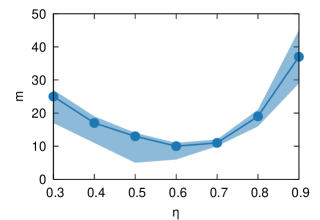
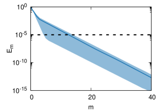
Figure 3: Equilibration of particles on a sphere at resolution $R/h=4$. The number of iterations required to reach the convergence criterion (10) with $\varepsilon_{p}=10^{-5}$ depending on the relaxation factor $\eta$ (top) and the convergence history for the difference after one iteration with $\eta=0.5$ (bottom). The lines show the median and the shades show the 10% and 90% percentiles over the interfacial cells.

2.5 Generalized height-function method

We compare our method with the generalized height-function method for curvature estimation implemented in Basilisk  [1, 29]. The algorithm attempts to compute the curvature in each interfacial cell with a series of techniques depending on the resolution. In three dimensions they can be outlined as follows

• Evaluate the height function along a preferred coordinate plane chosen based on the interface normal. The heights are obtained by summation over columns that span up to 13 cells. If consistent heights are available on the $3\times 3$ stencil, compute the curvature from them with finite differences.

• Collect heights from mixed directions in the $3\times 3\times 3$ stencil. If found six consistent heights, compute the curvature from a paraboloid fitted to them.

• If the curvature is already defined in one of the neighboring cells in the $3\times 3\times 3$ stencil, copy the curvature from the neighbor.

• Collect centroids of interfacial cells in the $3\times 3\times 3$ stencil. If found six centroids, compute the curvature from a paraboloid fitted to them.

• If all techniques fail, set the curvature to zero.

We refer to the documentation of Basilisk for further details of the algorithm. As clearly seen from the above description, the generalized height-function method, while providing an algorithm applicable at all resolutions, involves four different sources of curvature: heights, parabolic fitting to heights from mixed directions, values of curvature from neighboring cells and parabolic fit to centroids of the piecewise linear interface. Such procedure is complex for implementation and lacks robustness (e.g. depends on the presence of neighboring interfacial cells for parabolic fitting).

2.6 Combined particle and height-function method

As shown in Section 3, the error of our method asymptotically approaches a constant. To achieve second-order convergence, we follow the idea of the generalized height-function method and switch to standard heights at high resolutions. Our combined method therefore consists of two steps

• Evaluate the height function along a preferred coordinate plane chosen based on the interface normal. If consistent heights are available on a $3\times 3$ stencil, compute the curvature from them with finite differences.

• Otherwise, compute the curvature using the proposed particle method as described in Section 2.3.

Overall, the logic of the algorithm has greatly simplified compared to the generalized height function method. At the same time, as we demonstrate in the following sections, the combined method provides better accuracy at low resolutions and second-order convergence for well-resolved interfaces.

2.7 Sensitivity to parameters

Estimation of the interface curvature in three dimensions depends on three parameters: the number of particles per string $N$, the number of cross sections $N_{s}$ and the string length $H_{p}$. We set the parameters to $N=7$, $N_{s}=3$ and $H_{p}=4$. Then, we vary each parameter independently and examine their influence by estimating the curvature of a sphere at various resolutions following the test case in Section 3.1. The figures present the median error over 100 samples for the center from a uniform distribution over the octant of the cell, i.e. each coordinate is sampled from the range $[0,h/2]$. As seen from Figure 4, the number of particles has a minor influence on the result. Nevertheless, we observe that $N=3$ provides a two times larger error for bubbles at resolutions about one cell per radius. The influence of $N_{s}$ in Figure 5 is also small which is expected for a sphere. However, more complex shapes such as those observed during the bubble coalescence in Section 4.3, require at least $N_{s}=3$ as shown in Figure 7. Figure 6 shows a stronger influence of the string length $H_{p}$. Increasing the value from $H_{p}=2$ to $H_{p}=4$ reduces the error by a factor of ten.

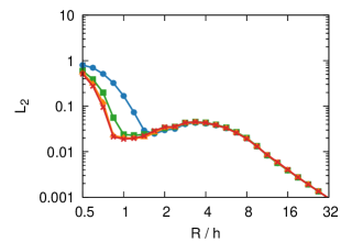
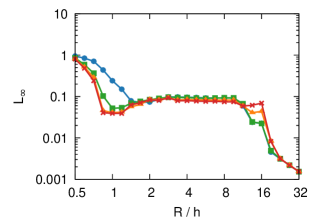
Figure 4: Curvature error for a sphere in $L_{2}$ and $L_{\infty}$ norms depending on the resolution for various values of the number of particles $N=3$ , $5$ , $7$  and $9$ .

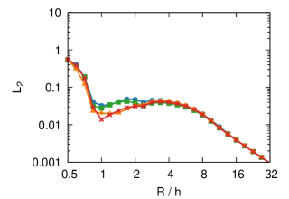
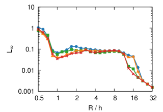
Figure 5: Curvature error for a sphere in $L_{2}$ and $L_{\infty}$ norms depending on the resolution for various values of the number of cross sections $N_{s}=1$ , $2$ , $3$  and $4$ .

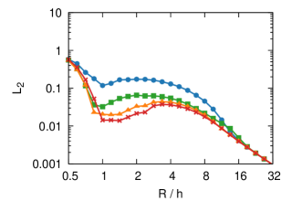
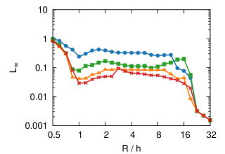
Figure 6: Curvature error for a sphere in $L_{2}$ and $L_{\infty}$ norms depending on the resolution for various values of the particle string length $H_{p}=2$ , $3$ , $4$  and $5$ .

            $N_{s}=1$             $N_{s}=2$             $N_{s}=3$             $N_{s}=4$

Figure 7: Isosurfaces of the volume fraction with $R/h=19.2$ at $t/T=0.08$ depending on the number of cross sections $N_{s}=1$, $2$, $3$ and $4$.

2.8 Computational cost

We compare the computational cost of our method to that of the generalized height-function method on the test case with a Taylor-Green vortex introduced in Section 4.1. The formulation is modified to consider 890 spherical bubbles at resolution $R/h=4$ on a mesh of $256^{3}$ cells. The initial positions of bubbles are distributed uniformly in the domain. The computations have been performed in parallel with 512 cores on Piz Daint supercomputer, where each compute node is equipped with a 12-core CPU Intel® Xeon® E5-2690 v3. Table 1 reports the runtime for both methods. About 5% of the cells contain interface fragments and require the curvature estimation. The time spent on the curvature estimation with the present method amounts to 125 ms per step or 31.1% of total time, while GHF takes 33 ms per step or 10.2% of total time. Therefore, our method is about four times more computationally expensive than GHF.

The cost of our method depends on the number of iterations and the number of particles per cell, which is controlled by parameters $N$, $N_{s}$ and $\varepsilon_{p}$. Estimation of curvature for a given volume fraction field consists of two parts: extraction of line segments and iterations. Extraction of the line segments from neighboring cells takes about 40% of the time and scales linearly with $N_{s}$. Iterations for equilibration of particles take about 60% of the time and scale linearly with $N_{s}\,N$.

	present	GHF
total time, per step	403 ms	329 ms
curvature estimation time, per step	125 ms	33 ms
curvature estimation time, to total time	31.1%	10.2%
cells containing interface, to all cells	5.17%	5.04%
cells with curvature from height functions, to all cells	0.69%	0.65%

Table 1: Runtime of the Taylor-Green vortex with 890 bubbles at resolution $R/h=4$ on a mesh of $256^{3}$. The benchmark is executed on Piz Daint with 512 cores. The runtime of one time step is averaged over all steps, and the number of interfacial cells is measured at the final time $t=10$.

3 Test cases

We examine the capabilities of the proposed method on two and three-dimensional benchmark problems: curvature of a sphere, a static droplet and a translating droplet. The volume fraction is initialized by the exact volume cut by a sphere (circle) [36].

3.1 Curvature

The volume fraction field represents a single sphere (circle) of radius $R$. We vary the number of cells per radius $R/h$ and consider 100 samples for the center from a uniform distribution over the octant (quadrant) of the cell, i.e. sampling each coordinate from the range $[0,h/2]$. We compute the relative curvature error in $L_{2}$ and $L_{\infty}$ norms

$$L_{2}(\kappa) =\Big{(}\frac{1}{|I|}\sum_{i\in I}\Big{(}\frac{\kappa_{i}-\kappa_{\text{ex}}}{\kappa_{\text{ex}}}\Big{)}^{2}\Big{)}^{1/2},$$ (14)

$$L_{\infty}(\kappa) =\max_{i\in I}\Big{|}\frac{\kappa_{i}-\kappa_{\text{ex}}}{\kappa_{\text{ex}}}\Big{|},$$ (15)

where $I$ is the indices of cells containing the interface (i.e. cells $i$ for which $0<\alpha_{i}<1$) and $\kappa_{\text{ex}}$ is the exact curvature (i.e. $\kappa_{\text{ex}}=2/R$ for sphere and $\kappa_{\text{ex}}=1/R$ for circle).

Figure 10 shows the error in comparison to GHF. At low resolutions, our method is more accurate in terms of the $L_{2}$-error up to eight cells per radius in 3D (and four cells in 2D) and at resolutions below two cells per radius the error is a factor of ten smaller. The method of particles alone as described in Section 2.3 does not converge at high resolutions, and the maximum error saturates at about 10%. The combined method from Section 2.6 switches to height functions at high resolutions and therefore converges with second order. Figures 8-9 show examples of final configuration of particles at resolutions below two cells per radius.

Figure 8: Line segments of the interface (black) and positions of particles (orange) from one selected cell for a circle at resolutions $R/h=0.59,\;0.71,\;0.84,\;1.0\;\text{and}\;1.19$. The central particle is highlighted by a thicker edge.

Figure 9: Polygons of the interface, cross sections (black) in case $N_{s}=2$ and positions of particles (orange) from one selected cell for a sphere at resolutions $R/h=0.59,\;0.71,\;0.84,\;1.0\;\text{and}\;1.19$.

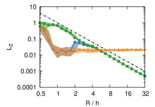
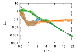
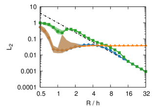
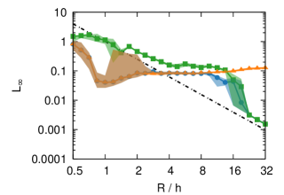
Figure 10: Curvature error for a circle (top) and sphere (bottom) in $L_{2}$ and $L_{\infty}$ norms depending on the resolution: particles only , combined particles and heights , GHF  and second-order convergence . The lines show the median and the shades show the 10% and 90% percentiles for random positions of the center.

3.2 Static droplet

We apply the model described in Section 2.1 for a spherical (circular) droplet in equilibrium. The initial velocity is zero and the volume fraction field represents a single sphere (circle) of radius $R$. We assume that both components have the same density and viscosity such that $\rho_{1}=\rho_{2}=\rho$ and $\mu_{1}=\mu_{2}=\mu$. This leaves one dimensionless parameter, the Laplace number characterizing the ratio between the surface tension, inertial and viscous forces

$$\text{La}=\frac{2\sigma\rho R}{\mu^{2}},$$ (16)

which we set to $\text{La}=1200$. We solve the problem on a mesh of $128^{3}$ cells (or $128^{2}$ cells in 2D) placing the droplet center in the corner and imposing the symmetry conditions on the adjacent boundaries. The other boundaries are free-slip walls. We vary the number of cells per radius $R/h$ and advance the solution until time $T=\rho(2R)^{2}/\mu$.

In the exact solution, the velocity remains zero and the pressure experiences a jump at the interface given by the Laplace pressure $p_{L}=\sigma\kappa_{\text{ex}}$. The numerical solutions develop spurious currents due to an imbalance between the pressure gradient and surface tension. We compute the magnitude of the spurious velocity in the $x$-direction

$$U_{\text{max}}=\max_{i\in C}|u_{x,i}|,$$ (17)

the corresponding Weber number

$$\text{We}_{\text{max}}=\frac{2\rho R{U}_{\text{max}}^{2}}{\sigma}$$ (18)

and the pressure jump

$$\Delta p=\max_{i\in C}p_{i}-\min_{i\in C}p_{i},$$ (19)

where $C$ is the indices of all cells.

Figures 11-12 show the values of $\text{We}_{\text{max}}$ and the relative pressure jump $\Delta p/p_{L}$ at $t=T$ depending on the resolution. The evolution of $\text{We}_{\text{max}}$ for two selected resolutions is shown in Figure 13. We observe that the solutions from GHF convergence with time to a zero spurious flow in most cases. This demonstrates the existence of a volume fraction field for which the method of height functions provides a uniform curvature field. In other cases, such as $R/h=2$ and $26.9$ in 3D, the spurious flow does not converge to zero. Meanwhile, our method of particles more accurately predicts the pressure jump at low resolutions below $R/h=4$ cells in 3D (and 3.36 cells in 2D) and provides lower magnitude of the spurious flow in cases such as $R/h=2$ in 3D shown in Figure 13.

We note, however, that the equilibration of a static droplet is largely of theoretical interest as the equilibrium shape is symmetric and aligned with the mesh directions. Such conditions are incompatible with advection and therefore rarely observed in practically relevant simulations. The spurious flow occurs in a more realistic scenario such as the translating droplet case discussed in Section 3.3.

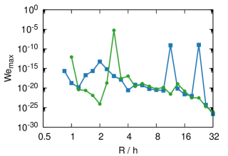
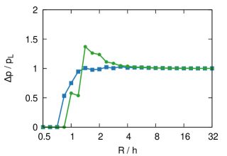
Figure 11: Velocity error and the pressure jump for a static droplet in 2D depending on the resolution: present  and GHF .

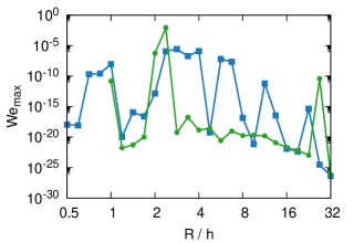
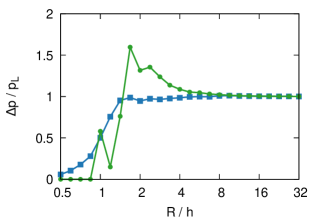
Figure 12: Velocity error and the pressure jump for a static droplet in 3D depending on the resolution: present  and GHF .

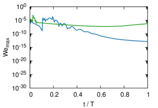
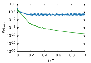
Figure 13: Evolution of the velocity error for a static droplet in 3D at resolutions $R/h=2$ (left) and $4$ (right): present  and GHF .

3.3 Translating droplet

We extend the previous case by adding a uniform initial velocity field $\bm{u}(\bm{x},0)=\bm{U}=U\bm{l}/|\bm{l}|$ where $\bm{l}=(1,\;0.8,\;0.6)$ in 3D and $\bm{l}=(1,\;0.8)$ in 2D. The additional parameter of the problem is the Weber number

$$\text{We}=\frac{2\rho RU^{2}}{\sigma},$$ (20)

which we set to $\text{We}=0.1$ while keeping $\text{La}=1200$. We solve the problem in a periodic domain on a mesh of $128^{3}$ cells (or $128^{2}$ cells in 2D). We vary the number of cells per radius $R/h$ and advance the solution until time $T=2R/U$.

The magnitude of the spurious flow is computed relative to the initial velocity as the maximum over all cells

$$U_{\text{max}}=\max_{i\in C}|u_{x,i}-U_{x}|$$ (21)

and definitions of $\text{We}_{\text{max}}$ and $\Delta p$ follow (18) and (19). Figures 14-15 show $\text{We}_{\text{max}}$ and the relative pressure jump $\Delta p/p_{L}$ depending on the resolution. The quantities are averaged over $t\in[T/2,T]$ and the evolution of $\text{We}_{\text{max}}$ for two selected resolutions is shown in Figure 16. Our method provides lower magnitudes of the spurious flow than GHF and more accurate values of the pressure jump at resolutions below $R/h=2.82$ cells in 3D (and $R/h=2$ cells in 2D), and at higher resolutions the error is comparable to GHF. We note that more accurate estimates of curvature in Section 3.1 are observed at similar resolutions.

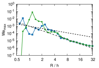
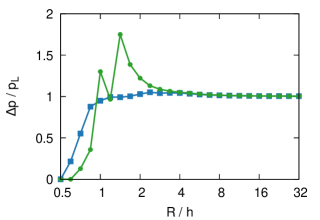
Figure 14: Velocity error and the pressure jump for a translating droplet in 2D depending on the resolution: present  and GHF . Convergence with first  and second  order.

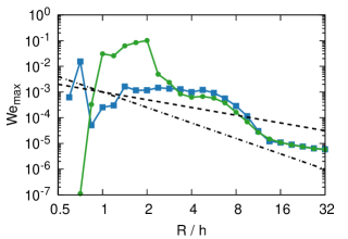
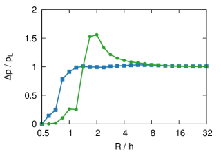
Figure 15: Velocity error and the pressure jump for a translating droplet in 3D depending on the resolution: present  and GHF . Convergence with first  and second  order.

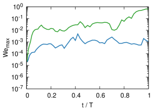
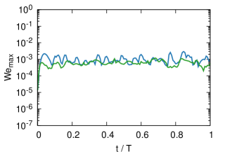
Figure 16: Evolution of the velocity error for a translating droplet in 3D at resolutions $R/h=2$ (left) and $4$ (right): present  and GHF .

4 Applications

4.1 Taylor-Green vortex with bubble

The Taylor-Green vortex is a classical benchmark for the capabilities of flow solvers to simulate single-phase turbulent flows [40]. Here we extend the formulation by adding a gaseous phase. The problem is solved in a periodic domain $[0,2\pi]^{3}$ with the initial velocity

$$\begin{split}u_{x}&=\sin x\;\cos y\;\cos z,\\ u_{y}&=-\cos x\;\sin y\;\cos z,\\ u_{z}&=0\end{split}$$ (22)

and a single bubble of radius $R=0.1$ placed at $(2,2,2)$. Parameters of the problem are the Reynolds number $\text{Re}=\rho_{1}/\mu_{1}$ and the Weber number $\text{We}=2\rho_{1}R/\sigma$. Here we choose $\text{Re}=800$ and $\text{We}=2$. The density and viscosity ratios are set to $\rho_{2}/\rho_{1}=0.01$ and $\mu_{2}/\mu_{1}=0.01$.

Figure 17 shows the trajectory of the bubble at various resolutions in comparison to GHF. Both methods converge to the same solution with the mesh refinement. However, at lower resolutions $R/h\leq 3.06$ our method provides qualitatively more accurate trajectories, while in GHF the trajectory is dominated by the spurious flow. Snapshots of the vorticity magnitude and the bubble shape are shown for both methods at $R/h=3.06$ in Figure 18

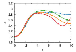
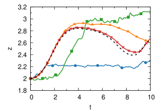
Figure 17: Trajectory of the bubble center of mass in the $z$-direction at various resolutions $R/h=$ $1.53$ , $2.04$ , $3.06$  and $4.08$ : present (left) and GHF (right). The dashed line  on the right shows the trajectory at $R/h=4.08$ from the present method.

Figure 18: Isosurfaces of the volume fraction and the magnitude of vorticity (increasing values from blue to red) with $R/h=2.04$ at $t=1.0,\;3.5,\;6.0\;\text{and}\;8.5$. At such resolution GHF (bottom) produces a solution with stronger spurious flow near the bubble than our method (top).

4.2 Taylor-Green vortex with elongated droplet

To evaluate our method on non-spherical shapes, we consider the Taylor-Green vortex with a droplet initially elongated in the $z$-direction. We use the same initial conditions (22) for the velocity field and define the volume fraction to describe a single elliptical droplet with $R=0.1$

$$\Big{(}\frac{x-2}{R}\Big{)}^{2}+\Big{(}\frac{y-2}{R}\Big{)}^{2}+\Big{(}\frac{z-2}{5R}\Big{)}^{2}=1.$$ (23)

The density and viscosity ratios are set to $\rho_{2}/\rho_{1}=10$ and $\mu_{2}/\mu_{1}=10$. Other parameters of the problem are kept the same: the Reynolds number $\text{Re}=\rho_{1}/\mu_{1}=800$ and the Weber number $\text{We}=2\rho_{1}R/\sigma=2$.

The deformation of the droplet is characterized by the gyration tensor

$$\frac{1}{V}\int(\bm{x}-\bm{x}_{c})\otimes(\bm{x}-\bm{x}_{c})\,\alpha\,dV,$$ (24)

where $V=\int{\alpha\,dV}$ and $\bm{x}_{c}=\frac{1}{V}\int{\bm{x}\alpha\,dV}$. For an elliptical droplet, the principal components $\lambda_{1}<\lambda_{2}<\lambda_{3}$ of the gyration tensor relate to semi-axes $R_{1}<R_{2}<R_{3}$ of the ellipsoid as $R_{i}=\sqrt{5\lambda_{i}},\;i=1,2,3$. Figure 19 shows the trajectory of the droplet center of mass in the $z$-direction and the smallest semi-axis $R_{1}$ of the ellipsoid of gyration at various resolutions in comparison to GHF. Snapshots of the vorticity magnitude and the bubble shapes are shown in Figures 20-21 for both methods at resolutions $R/h=1.53$ and $4.08$. Both methods converge to the same solution with the mesh refinement. The oscillation of the droplet is indicated by $R_{1}(t)$ which starts at $R_{1}=0.1$ according the initial conditions and reaches the first maximum at $t=1.2$ when the droplet approaches a spherical shape shown in Figure 21. Due to inertia, the droplet further deforms to an oblate shape corresponding to a minimum of $R_{1}$ at $t=1.5$. At the lowest resolution $R/h=1.53$, our method captures the formation of the oblate shape at $t=1.8$ which is delayed compared to the finest resolution. However, with GHF the oblate shape is not captured. At the next resolution $R/h=2.04$, GHF computes the trajectory more accurately than our method.

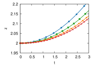
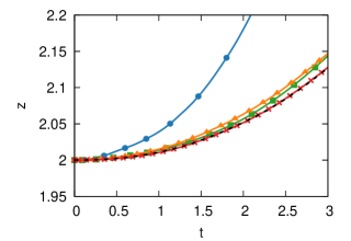
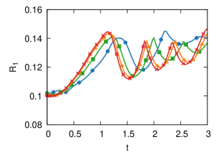
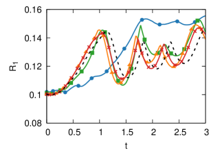
Figure 19: Trajectory of the droplet center of mass in the $z$-direction and the smallest semi-axis of the ellipsoid of gyration at various resolutions $R/h=$ $1.53$ , $2.04$ , $3.06$  and $4.08$ : present (left) and GHF (right). The dashed line  on the right shows the results at the finest resolution $R/h=4.08$ by the present method.

Figure 20: Isosurfaces of the volume fraction and the magnitude of vorticity (increasing values from blue to red) with resolution $R/h=1.53$ at $t=$0.0, 0.3, 0.6, 0.9, 1.2, 1.5 and 1.8: present method (top) and GHF (bottom). Unlike GHF, our method captures the oblate shape at $t=1.5$.

Figure 21: Isosurfaces of the volume fraction and the magnitude of vorticity (increasing values from blue to red) with resolution $R/h=4.08$ at $t=$0.0, 0.3, 0.6, 0.9, 1.2, 1.5 and 1.8: present method (top) and GHF (bottom).

4.3 Coalescence of bubbles

Coalescence of bubbles and drops is an actively studied phenomenon commonly found in nature and industry [5, 35]. Here we consider coalescence of two spherical bubbles. The problem is solved in a periodic domain $[0,1]^{3}$ with zero initial velocity and two tangent bubbles of radius $R=0.15$ placed along the $x$-axis. The only parameter of the problem is the Ohnesorge number

$$\text{Oh}=\frac{\mu_{1}}{\sqrt{\rho_{1}R\sigma}},$$ (25)

which we set to $\text{Oh}=0.007$. The density and viscosity ratios are set to $\rho_{2}/\rho_{1}=0.01$ and $\mu_{2}/\mu_{1}=0.01$.

We refer to [35] for a detailed experimental study of bubble coalescence. The process starts with the formation of a neck connecting the bubbles which then propagates along the bubble surface. Figures 22-23 show the isosurfaces of the volume fraction with different resolutions at $t/T=0.08$ and $0.18$, where $T=\sqrt{\rho_{1}R^{3}/\sigma}$ is the capillary time.

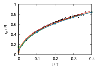
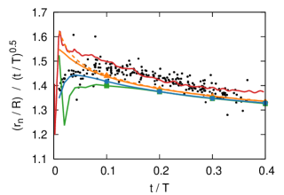
Figure 31: Evolution of the coalescence neck radius relative to the bubble radius (left) and the coalescence neck radius divided by $\sqrt{t}$ (right). Gerris in the axisymmetric formulation with adaptive mesh refinement with the equivalent resolution $R/h=307.2$  and $R/h=614.4$ , Basilisk with proposed method for curvature at $R/h=38.4$  and Aphros at $R/h=153.6$ . Experiment [35] (dots) and boundary integral [35]  without scaling of time.

We found that shapes from our simulations match well the experimental results (see Figures 22, 23 and 29) when a factor of 1.2 is applied to the values of time reported in [35]. We note that the simulations using the boundary integral method [35] capture the shapes reported in experiments without mentioning any such factor. We performed additional simulations using Gerris [29] (see Figure 31) and again matching shapes obtained by these simulations and those obtained experimentally required the adjustment by the factor of 1.2, in agreement with Basilisk and our own software. This discrepancy may be attributed to the use of an inviscid boundary integral method in [35] and the viscous simulations employed in Gerris, Basilisk and our own software. Furthermore, we match the results of another experimental study [39] without scaling of time as shown in Section A2 and Figures 32-33.

The evolution of the neck radius is presented in Figure 24 in comparison to the experimental data reported in [35]. We observe that the present method agrees well with experimental data while this is not the case for simulations using the generalized height function method, in particular at later times (see Figure 23). The generalized height-function method introduces spurious disturbances of the interface near the coalescence neck. Furthermore, its solution does not converge with mesh refinement. The reason for this is that the initial shape has effectively infinite curvature at the coalescence neck as refining the mesh increases the curvature resolved on the mesh. As seen from Figure 25, increasing the resolution reduces the percentage of cells where height functions are not defined and the curvature is estimated using particles. Nevertheless, more accurate estimation of curvature in such cells benefits the overall accuracy.

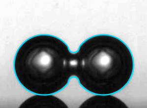
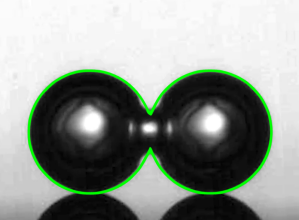
Figure 22: Isosurfaces of volume fraction at $t/T=0.08$ depending on resolution $R/h=9.6$ (top), $19.2$ (middle) and $38.4$ (bottom): present (left) and GHF (right). Experimental image [35] overlapped with contours from the finest mesh of each method. The time value for the experimental image is multiplied by 1.2.

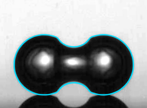
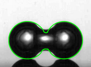
Figure 23: Isosurfaces of volume fraction at $t/T=0.18$ depending on resolution $R/h=9.6$ (top), $19.2$ (middle) and $38.4$ (bottom): present (left) and GHF (right). Experimental image [35] overlapped with contours from the finest mesh of each method. The time value for the experimental image is multiplied by 1.2.

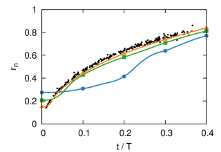
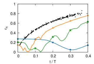
Figure 24: Evolution of the neck radius depending on the resolution $R/h=9.6$ , $19.2$ , $38.4$ : present (left) and GHF (right) compared to experiment [35] (dots).

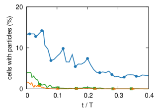
Figure 25: Percentage of interfacial cells where the curvature is computed with particles for $R/h=9.6$ , $19.2$ , $38.4$ .

4.4 Breakup of air sheet in shear flow

The following test case demonstrates the deformation and breakup of an air sheet in shear flow. The domain $[0,2]\times[0,1]\times[0,1]$ is periodic in the $x$- and $z-$directions and no-slip conditions are imposed on the boundaries in the $y$-direction. The initial velocity profile is simple shear $u_{x}=(y-0.5)U/D$ and $u_{y}=u_{z}=0$, where $D=0.05$ is the thickness of the sheet and $U=0.2$ is the velocity difference. The initial volume fraction

$$\alpha=\begin{cases}1,&\big{|}\,0.1\sin(\pi x)\sin(2\pi z)+0.5-y\big{|}<\frac{D}{2}\\ 0,&\text{otherwise}\end{cases}$$ (26)

is shown in Figure 26. Parameters of the problem are the Reynolds number $\text{Re}=\rho_{1}UD/\mu_{1}$ and the Weber number $\text{We}=\rho_{1}U^{2}D/\sigma$. Here we choose $\text{Re}=80$ and $\text{We}=0.64$. The density and viscosity ratios are set to $\rho_{2}/\rho_{1}=0.01$ and $\mu_{2}/\mu_{1}=0.01$.

Initial deformations of the air sheet develop further in the shear flow. This leads to tearing of the interface starting in four distinct locations. Figure 27 shows the shapes computed with both methods of curvature estimation at various resolutions. Both methods converge to the same solution with mesh refinement. At lower resolutions, GHF shows more tearing of the interface, while with the present method the interface remains stable.

\begin{overpic}[unit=1mm,scale={0.172}]{shear/view/scheme/a_0000.png} \put(0.0,22.0){\includegraphics[width=56.9055pt]{shear/view/scheme/scheme.pdf}} \end{overpic}

Figure 26: Initial volume fraction representing an air sheet. Arrows indicate the direction of the shear.

\begin{overpic}[unit=1mm,scale={0.172}]{shear/view/bap128/a_0017.png} \put(1.0,26.0){present, $D/h=3.2$} \end{overpic}

\begin{overpic}[unit=1mm,scale={0.172}]{shear/view/ba128/a_0017.png} \put(1.0,26.0){GHF, $D/h=3.2$} \end{overpic}

\begin{overpic}[unit=1mm,scale={0.172}]{shear/view/bap256/a_0017.png} \put(1.0,26.0){present, $D/h=6.4$} \end{overpic}

\begin{overpic}[unit=1mm,scale={0.172}]{shear/view/ba256/a_0017.png} \put(1.0,26.0){GHF, $D/h=6.4$} \end{overpic}

\begin{overpic}[unit=1mm,scale={0.172}]{shear/view/bap512/a_0017.png} \put(1.0,26.0){present, $D/h=12.8$} \end{overpic}

\begin{overpic}[unit=1mm,scale={0.172}]{shear/view/ba512/a_0017.png} \put(1.0,26.0){GHF, $D/h=12.8$} \end{overpic}

Figure 27: Shapes of the air sheet at $t=1.7$ computed with present method (left) and GHF (right) at resolutions $D/h=$3.2 (top), 6.4 (middle) and 12.8 (bottom).

5 Conclusion

We have presented a new method for estimating the curvature of the interface by fitting circular arcs to its piecewise linear reconstruction. The circular arcs are represented as strings of particles which evolve under constraints and forces attracting them to the interface.

The application of the method on a number of benchmark problems shows a significant improvement in the accuracy of computing the curvature of interfaces at low resolutions over the generalized height-function method [29] implemented in Basilisk [1]. The present method is more accurate at resolutions up to four cells per curvature radius and even with one cell per radius provides the relative curvature error below 10%. We also demonstrate the capabilities of this hybrid method on a number of applications including multiphase vortical flows and bubble coalescence. Further applications include the bubble dynamics in electrochemical cells [19] and a plunging jet with air entrainment [21].

The present technique restricts the particles to circular arcs and computes the attraction force from the nearest point on the interface. However, the method allows for modifications of the constraints and forces. For instance, the force can be computed directly from the volume fraction using the area cut by the string of particles. Forces defined from the intersection with the reconstructed volume can lead to an approach similar to the mesh-decoupled height functions [27]. Finally, the property of recovering the exact curvature mentioned in Section A1 can contribute to the existence of volume fraction fields providing a uniform curvature field and, therefore, exact equilibration of a static droplet. Such modifications constitute the subject of future work.

6 Acknowledgements

This research is funded by grant no. CRSII5_173860 of the Swiss National Science Foundation. The authors acknowledge the use of computing resources from CSCS (projects s754 and s931). We thank Professor Georges-Henri Cottet (Grenoble, France) for several helpful discussions regarding this work.

Appendix A

A1 Attraction to circular arcs

The attraction force (7) can be modified to include a dependency on the current estimate of curvature. One such modification consists in replacing the line segments with circular arcs. This formulation recovers the exact curvature if the endpoints of all line segments belong to a circle. To define the force at position $\bm{x}$, we find the nearest point $\bm{y}\in L$ on the interface and the corresponding line segment $[\bm{a}_{l},\bm{b}_{l}]$. Then we find a factor $\delta$ such that

$$\bm{x}_{L}(\bm{x},\kappa)=\bm{y}+\delta\bm{n}_{l}$$ (27)

belongs to a circular arc of curvature $\kappa$ through the endpoints $\bm{a}_{l}$ and $\bm{b}_{l}$, where $\kappa$ is a known estimation of curvature and $\bm{n}_{l}$ is the unit normal of $[\bm{a}_{l},\bm{b}_{l}]$. Such $\delta$ is given by

$$\delta=\sqrt{\tfrac{1}{\kappa^{2}}-d^{2}}-\sqrt{\tfrac{1}{\kappa^{2}}-w^{2}}=\frac{\kappa(w^{2}-d^{2})}{\sqrt{1-\kappa^{2}d^{2}}+\sqrt{1-\kappa^{2}w^{2}}},$$ (28)

where $d=|\bm{y}-\bm{c}_{l}|$, $w=|\bm{a}_{l}-\bm{c}_{l}|$ and $\bm{c}_{l}=(\bm{a}_{l}+\bm{b}_{l})/2$. Finally, the force is defined as

$$\bm{f}(\bm{x},\kappa)=\eta\;\big{(}\bm{x}_{L}(\bm{x},\kappa)-\bm{x}\big{)},$$ (29)

where $\eta\in[0,\,1]$ is a relaxation parameter. Figure 28 illustrates the computation of forces after replacing the line segments with circular arcs.

Figure 28: Line segments represent the interface and circular arcs of curvature $\kappa$ pass through their endpoints. The force acts on each particle towards the circular arc from the nearest line segment.

A2 Coalescence of bubbles with SIMPLE-based solver

The method for curvature estimation is also implemented as part of our in-house multiphase flow solver Aphros. We use a finite volume discretization based on the SIMPLE method for the pressure coupling [28, 17] and the second-order scheme QUICK [25] for convective fluxes. The advection equation is solved using the volume-of-fluid method PLIC with piecewise linear reconstruction [7], where the normals are computed using the mixed Youngs-centered scheme which is a combination of Youngs’ scheme and the height functions. The cell-centered interface curvature $\kappa$ is computed from the volume fraction using the proposed method. Our approximation of the surface tension force is well-balanced [18] (i.e. the surface tension force is balanced by the pressure gradient if the curvature is uniform) and requires face-centered values of the curvature which are taken from the neighboring cell with minimal $|\alpha-\tfrac{1}{2}|$.

The algorithm is implemented on top of Cubism [42, 2], an open-source C++ framework for distributed parallel solvers on structured grids. To solve the linear systems, we use the GMRES method [32] for the momentum equation and the preconditioned conjugate gradient method [6] for the pressure correction implemented in the Hypre library [3, 16].

One functionality of our code is the ability to describe static contact angles of $0$ and $180$ degrees. This feature is implemented using ghost cells. Assuming that $\alpha=1$ is the volume fraction inside the bubble or droplet, we fill two layers of ghost cells adjacent to boundaries with values $\alpha=0$ and $\alpha=1$ for the contact angles of $180$ and $0$ degrees respectively. Based on such volume fraction field, we estimate the normals and curvature in all domain cells with the usual algorithm. This allows us to describe the evolution of the two bubbles after coalescence presented in Section 4.3 at later stages as well and include the detachment from the solid wall and oscillations. The problem formulation is closer to the experimental conditions than in Section 4.3. The bubbles are initially placed near a solid wall with the imposed contact angle of 180 degrees and the gravitational acceleration is considered with the Eötvös number of $\text{Eo}=\rho gR^{2}/\sigma=0.061$. Results of the simulation compared to the experimental images are shown in Figure 29.

Furthermore, the evolution of the coalescence neck radius on the coarsest resolution is more accurate than in Basilisk as shown in Figures 24 and 30. This is attributed to differences in the algorithm for computation of interface normals and the way the estimates of curvature are transferred from cells to faces (average over neighbors in Basilisk, and the cell with the minimal $|\alpha-\tfrac{1}{2}|$ in Aphros).

We have also considered another experimental study of bubble coalescence [39]. Initially, both bubbles are positioned along the $z$-axis and have elliptical shapes. One bubble with semi-axes $R_{x}=R_{y}=1.08\,R$ and $R_{z}=1.0\,R$ is positioned above the other bubble with semi-axes $R_{x}=R_{y}=0.92\,R$ and $R_{z}=0.97\,R$, where $R$ is their characteristic size. The Ohnesorge number $\text{Oh}=\frac{\mu_{1}}{\sqrt{\rho_{1}R\sigma}}$ is set to $\text{Oh}=0.007$. The experimental images overlaid with the results of the simulation are shown in Figure 32 and the evolution of coalescence neck is presented in Figure 33. In this case, our results agree with the experimental data without scaling of time.

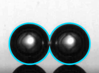
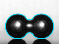
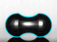
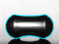
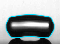
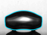
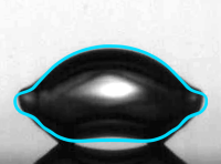
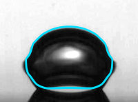
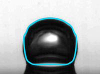
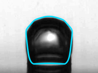
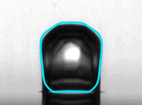
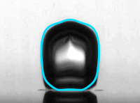
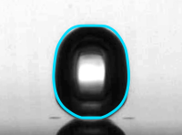
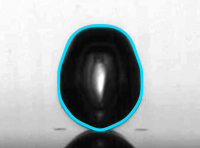
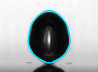
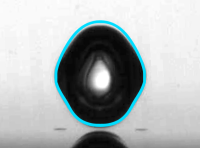
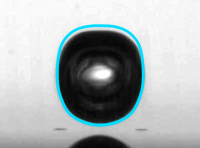
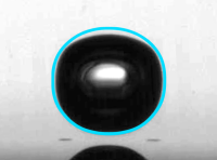
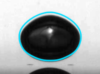
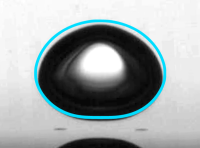
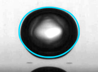
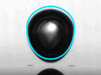
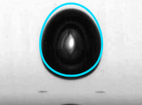
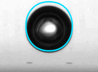
Figure 29: Snapshots from experiment [35] overlaid by the projections of the shapes from the simulation by Aphros with resolution $R/h=76.8$ (blue lines) at times $t/T=$ 0, 0.13, 0.26, 0.4, 0.53, 0.66, 0.79, 0.92, 1.1, 1.2, 1.3, 1.4, 1.6, 1.7, 1.8, 2.1, 2.4, 2.6, 2.9, 3.2, 3.7, 4.2, 4.7 and 5.3. The time values for the experimental images are multiplied by 1.2.

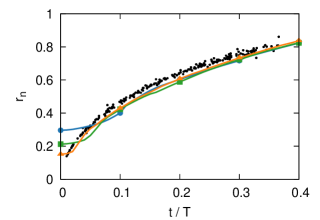
Figure 30: Evolution of the coalescence neck radius relative to the bubble radius depending on the resolution $R/h=9.6$ , $19.2$  and $38.4$  produced by Aphros compared to experiment [35] (dots).

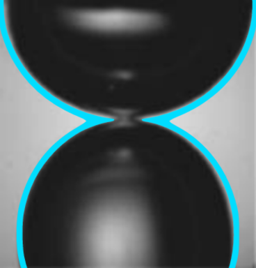
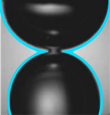
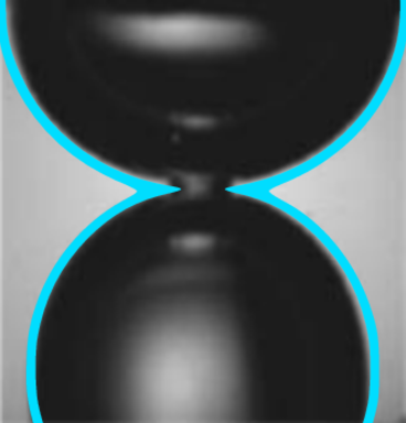
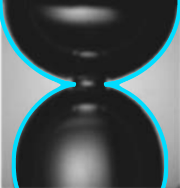
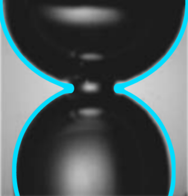
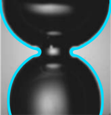
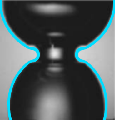
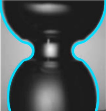
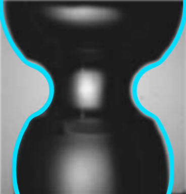
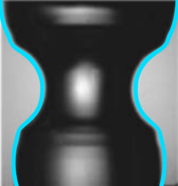
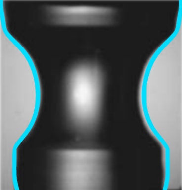
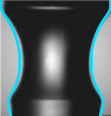
Figure 32: Snapshots from experiment [39] overlaid by the projections of the shapes from the simulation by Aphros with resolution $R/h=76.8$ (blue lines) at times $t/T=$0, 0.0061, 0.012, 0.018, 0.031, 0.043, 0.061, 0.08, 0.12, 0.17, 0.21 and 0.27. Experimental images reprinted from [39], with the permission from AIP Publishing.

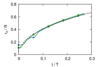
Figure 33: Evolution of the coalescence neck radius relative to the bubble radius depending on the resolution $R/h=38.4$  and $76.8$  produced by Aphros compared to experiment [39] (dots).

A3 Derivatives of particle positions

The algorithm in Section 2.2 requires derivatives of particle positions (5) with respect to angles $\phi$ and $\theta$ which are given as

$$\frac{\partial\bm{x}_{i}}{\partial\phi}=\begin{cases}\sum\limits_{j=1}^{i-c}h_{p}\bm{e}\big{(}\phi+(j-\frac{1}{2})\,\theta+\frac{\pi}{2}\big{)}&\qquad i>c,\\ \bm{0}&\qquad i=c,\\ -\sum\limits_{j=1}^{c-i}h_{p}\bm{e}\big{(}\phi-(j-\frac{1}{2})\,\theta+\frac{\pi}{2}\big{)}&\qquad i<c,\end{cases}$$ (30)

$$\frac{\partial\bm{x}_{i}}{\partial\theta}=\begin{cases}\sum\limits_{j=1}^{i-c}h_{p}\big{(}j-\frac{1}{2}\big{)}\,\bm{e}\big{(}\phi+(j-\frac{1}{2})\,\theta+\frac{\pi}{2}\big{)}&\qquad i>c,\\ \bm{0}&\qquad i=c,\\ \sum\limits_{j=1}^{c-i}h_{p}\big{(}j-\frac{1}{2}\big{)}\,\bm{e}\big{(}\phi-(j-\frac{1}{2})\,\theta+\frac{\pi}{2}\big{)}&\qquad i<c,\end{cases}$$ (31)

The following recurrence relations are useful for the implementation:

$$\bm{x}_{i}=\begin{cases}\bm{x}_{i-1}+h_{p}\bm{e}\big{(}\phi+(i-c-\frac{1}{2})\,\theta\big{)}&\quad i>c,\\ \bm{p}&\quad i=c,\\ \bm{x}_{i+1}-h_{p}\bm{e}\big{(}\phi-(c-i-\frac{1}{2})\,\theta\big{)}&\quad i<c,\end{cases}$$ (32)

$$\frac{\partial\bm{x}_{i}}{\partial\phi}=\begin{cases}\frac{\partial\bm{x}_{i-1}}{\partial\phi}+h_{p}\bm{e}\big{(}\phi+(i-c-\frac{1}{2})\,\theta+\frac{\pi}{2}\big{)}&\quad i>c,\\ \bm{0}&\quad i=c,\\ \frac{\partial\bm{x}_{i+1}}{\partial\phi}-h_{p}\bm{e}\big{(}\phi-(c-i-\frac{1}{2})\,\theta+\frac{\pi}{2}\big{)}&\quad i<c,\end{cases}$$ (33)

$$\frac{\partial\bm{x}_{i}}{\partial\theta}=\begin{cases}\frac{\partial\bm{x}_{i-1}}{\partial\theta}+h_{p}(i-c-\frac{1}{2})\,\bm{e}\big{(}\phi+(i-c-\frac{1}{2})\,\theta+\frac{\pi}{2}\big{)}&\quad i>c,\\ \bm{0}&\quad i=c,\\ \frac{\partial\bm{x}_{i+1}}{\partial\theta}+h_{p}(c-i-\frac{1}{2})\,\bm{e}\big{(}\phi-(c-i-\frac{1}{2})\,\theta+\frac{\pi}{2}\big{)}&\quad i<c,\end{cases}$$ (34)

A4 Proof of convergence of iterations

We show that iterations in Section 2.2 can be formulated as steps of the gradient descent minimizing an energy function. Given the initial conditions, the central particle $\bm{x}_{c}$ already belongs to a line segment. Therefore, the corresponding force is zero $\bm{f}^{m}_{c}=0$, and Step 1 trivializes such that $\bm{p}^{m}=\bm{p}^{0}$, $\bm{X}^{*}=\bm{X}^{m}$ and $\bm{F}^{*}=\bm{F}^{m}$. In the following, the argument $\bm{p}$ is omitted. We define the energy in terms of the remaining parameters $\phi$ and $\theta$

$$E(\phi,\theta)=\frac{1}{2}\sum_{i=1}^{N}\min_{\bm{y}\in L}|\bm{y}-\bm{x}_{i}(\phi,\theta)|^{2}.$$ (35)

The energy can be expressed as a superposition

$$E(\phi,\theta)=\hat{E}(\phi,\theta,\bm{Y}_{\text{min}}(\phi,\theta))$$ (36)

of two functions

$$\hat{E}(\phi,\theta,\bm{Y})=\frac{1}{2}\sum_{i=1}^{N}|\bm{y}_{i}-\bm{x}_{i}(\phi,\theta)|^{2}$$ (37)

$$\bm{Y}_{\text{min}}(\phi,\theta)=[\operatorname*{arg\,min}_{\mathbf{y}\in L}|\bm{y}-\bm{x}_{i}(\phi,\theta)|,\;i=1,\dots,N].$$ (38)

Derivatives of $\hat{E}$ read

$$\frac{\partial\hat{E}}{\partial\phi}(\phi,\theta,\bm{Y})=-(\bm{Y}-\bm{X}(\phi,\theta))\cdot\frac{\partial\bm{X}}{\partial\phi}(\phi,\theta)$$

$$\frac{\partial\hat{E}}{\partial\theta}(\phi,\theta,\bm{Y})=-(\bm{Y}-\bm{X}(\phi,\theta))\cdot\frac{\partial\bm{X}}{\partial\theta}(\phi,\theta).$$

In this notation, the force defined by (7) and (9) transforms to

$$\bm{F}(\phi,\theta)=\eta\,\big{(}\bm{Y}_{\text{min}}(\phi,\theta)-\bm{X}(\phi,\theta)\big{)}.$$ (39)

Taking into account

$$\bm{F}^{*}\cdot\bm{D}_{\phi}=-\eta\frac{\partial\hat{E}}{\partial\phi}(\phi^{m},\theta^{m},\bm{Y}^{m})$$

$$\bm{F}^{*}\cdot\bm{D}_{\theta}=-\eta\Big{[}\frac{\partial\hat{E}}{\partial\theta}(\phi^{m+1},\theta^{m},\bm{Y}^{m})-\big{(}\bm{X}(\phi^{m+1},\theta^{m})-\bm{X}(\phi^{m},\theta^{m})\big{)}\Big{]}\,,$$

corrections in Step 2 and Step 3 can be expressed as

$$\phi^{m+1}=\phi^{m}-\frac{\eta}{\|\bm{D}_{\phi}\|^{2}}\frac{\partial\hat{E}}{\partial\phi}(\phi^{m},\theta^{m},\bm{Y}^{m})$$ (40)

$$\theta^{m+1}=\theta^{m}-\frac{\eta}{\|\bm{D}_{\theta}\|^{2}}\frac{\partial\hat{E}}{\partial\theta}(\phi^{m+1},\theta^{m},\bm{Y}^{m})\,-$$ (41)

$$-\frac{1-\eta}{\|\bm{D}_{\theta}\|^{2}}\big{(}\bm{X}(\phi^{m+1},\theta^{m})-\bm{X}(\phi^{m},\theta^{m})\big{)}\cdot\bm{D}_{\theta}\,,$$

where $\bm{F}^{*}=\bm{F}(\phi^{m},\theta^{m})$, $\bm{D}_{\phi}=\frac{\partial\bm{X}}{\partial\phi}(\phi^{m},\theta^{m})$, $\bm{D}_{\theta}=\frac{\partial\bm{X}}{\partial\theta}(\phi^{m+1},\theta^{m})$ and $\bm{Y}^{m}=\bm{Y}_{\text{min}}(\phi^{m},\theta^{m})$. The second correction can be rewritten

$$\theta^{m+1}=\theta^{m}-\frac{\eta}{\|\bm{D}_{\phi}\|^{2}}\frac{\partial\hat{E}}{\partial\theta}(\phi^{m+1},\theta^{m},\bm{Y}^{m})\,+$$ (42)

$$+\frac{(1-\eta)\eta\,\tilde{\bm{D}}_{\phi}\cdot\bm{D}_{\theta}}{\|\bm{D}_{\phi}\|^{2}\|\bm{D}_{\theta}\|^{2}}\frac{\partial\hat{E}}{\partial\phi}(\phi^{m},\theta^{m},\bm{Y}^{m})$$

in terms of the finite difference

$$\tilde{\bm{D}}_{\phi}=\frac{\bm{X}(\phi^{m+1},\theta^{m})-\bm{X}(\phi^{m},\theta^{m})}{\phi^{m+1}-\phi^{m}}.$$ (43)

Function $\hat{E}(\phi,\theta,\bm{Y})$ is smooth on a compact set $[0,2\pi]\times[0,2\pi]\times L^{N}$, and therefore its gradient is Lipschitz continuous. In particular, for a constant $\lambda>0$

$$\begin{split}\Big{|}\frac{\partial\hat{E}}{\partial\phi}(\phi+\Delta\phi,\theta,\bm{Y})-\frac{\partial\hat{E}}{\partial\phi}(\phi,\theta,\bm{Y})\Big{|}\leq\lambda\,\Delta\phi,\\ \Big{|}\frac{\partial\hat{E}}{\partial\theta}(\phi,\theta+\Delta\theta,\bm{Y})-\frac{\partial\hat{E}}{\partial\theta}(\phi,\theta,\bm{Y})\Big{|}\leq\lambda\,\Delta\theta.\end{split}$$ (44)

This implies that

$$\big{|}\Delta E-(E_{\phi}\Delta\phi+E_{\theta}\Delta\theta)\big{|}\leq\lambda(\Delta\phi^{2}+\Delta\theta^{2}),$$ (45)

where $\Delta\phi=\phi^{m+1}-\phi^{m}$, $\Delta\theta=\theta^{m+1}-\theta^{m}$, $\Delta E=\hat{E}(\phi^{m+1},\theta^{m+1},\bm{Y}^{m})-\hat{E}(\phi^{m},\theta^{m},\bm{Y}^{m})$, $E_{\phi}=\frac{\partial\hat{E}}{\partial\phi}(\phi^{m},\theta^{m},\bm{Y}^{m})$ and $E_{\theta}=\frac{\partial\hat{E}}{\partial\theta}(\phi^{m+1},\theta^{m},\bm{Y}^{m})$. Therefore, the change of the energy after both corrections is bounded as

$$\Delta E\leq E_{\phi}\Delta\phi+E_{\theta}\Delta\theta+\lambda(\Delta\phi^{2}+\Delta\theta^{2}).$$ (46)

We show that for a sufficiently small $\eta>0$,

$$E_{\phi}\Delta\phi+E_{\theta}\Delta\theta+\lambda(\Delta\phi^{2}+\Delta\theta^{2})\leq 0,$$ (47)

which, given (40) and (42), is equivalent to

$$-\bm{v}^{T}\bm{A}\bm{v}+\lambda\eta\,|\bm{A}\bm{v}|^{2}\leq 0,$$ (48)

where

$$\bm{A}=\begin{bmatrix}\frac{1}{\|\bm{D}_{\phi}\|^{2}}&0\\ -\frac{(1-\eta)\,\tilde{\bm{D}}_{\phi}\cdot\bm{D}_{\theta}}{\|\bm{D}_{\phi}\|^{2}\|\bm{D}_{\theta}\|^{2}}&\frac{1}{\|\bm{D}_{\theta}\|^{2}}&\end{bmatrix}\quad\bm{v}=\begin{bmatrix}E_{\phi}\\ E_{\theta}\end{bmatrix}.$$ (49)

This follows from a stronger inequality

$$-\bm{v}^{T}\bm{A}\bm{v}+\lambda\eta\,\|\bm{A}\|^{2}|\bm{v}|^{2}\leq 0$$ (50)

or, in terms of a symmetric matrix,

$$\bm{v}^{T}\Big{(}\frac{\bm{A}+\bm{A}^{T}}{2}-\lambda\eta\,\|\bm{A}\|^{2}\bm{I}\Big{)}\bm{v}\geq 0,$$ (51)

which states that the matrix is positive semi-definite. As seen from (30-31), derivatives $\bm{D}_{\phi}$ and $\bm{D}_{\theta}$ are uniformly bounded away from zero and infinity. Therefore, it is sufficient to show that matrix $\frac{\bm{A}+\bm{A}^{T}}{2}$ is positive definite in the limiting case $\eta\rightarrow 0$

$$\frac{\bm{A}+\bm{A}^{T}}{2}=\begin{bmatrix}\frac{1}{\|\bm{D}_{\phi}\|^{2}}&-\frac{1}{2}\frac{{\bm{D}}_{\phi}\cdot\bm{D}_{\theta}}{\|\bm{D}_{\phi}\|^{2}\|\bm{D}_{\theta}\|^{2}}\\ -\frac{1}{2}\frac{{\bm{D}}_{\phi}\cdot\bm{D}_{\theta}}{\|\bm{D}_{\phi}\|^{2}\|\bm{D}_{\theta}\|^{2}}&\frac{1}{\|\bm{D}_{\theta}\|^{2}}&\end{bmatrix}$$ (52)

as the finite difference $\tilde{\bm{D}}_{\phi}$ from (43) uniformly converges to $\bm{D}_{\phi}$. The above is equivalent to

$$\frac{\,({\bm{D}}_{\phi}\cdot\bm{D}_{\theta})^{2}}{\,\|\bm{D}_{\phi}\|^{2}\|\bm{D}_{\theta}\|^{2}}<4,$$ (53)

which always holds for a scalar product. This shows that corrections of parameters $\phi$ and $\theta$ reduce the energy

$$\hat{E}(\phi^{m+1},\theta^{m+1},\bm{Y}^{m})\leq\hat{E}(\phi^{m},\theta^{m},\bm{Y}^{m}).$$ (54)

Finally, definition (38) implies that

$$\hat{E}(\phi^{m+1},\theta^{m+1},\bm{Y}_{\text{min}}(\phi^{m+1},\theta^{m+1}))\leq\hat{E}(\phi^{m+1},\theta^{m+1},\bm{Y}^{m}).$$ (55)

Combining the last two inequalities, we arrive at

$$\hat{E}(\phi^{m+1},\theta^{m+1},\bm{Y}^{m+1})\leq\hat{E}(\phi^{m},\theta^{m},\bm{Y}^{m})$$ (56)

or, in the original notation (36),

$$E(\phi^{m+1},\theta^{m+1})\leq E(\phi^{m},\theta^{m}).$$ (57)

Together with $E\geq 0$, this guarantees convergence of iterations.

References

References

- [1] Basilisk. http://basilisk.fr/.
- [2] Cubism: Parallel block processing library. https://gitlab.ethz.ch/mavt-cse/Cubism.
- [3] HYPRE: Scalable linear solvers. https://computation.llnl.gov/projects/hypre-scalable-linear-solvers-multigrid-methods.
- [4] Aniszewski, W., Zaleski, S., Popinet, S., and Saade, Y. Planar Jet Stripping of Liquid Coatings: Numerical Studies. arXiv e-prints (Jul 2019), arXiv:1907.07659.
- [5] Anthony, C. R., Kamat, P. M., Thete, S. S., Munro, J. P., Lister, J. R., Harris, M. T., and Basaran, O. A. Scaling laws and dynamics of bubble coalescence. Physical Review Fluids 2, 8 (2017), 083601.
- [6] Ashby, S. F., and Falgout, R. D. A parallel multigrid preconditioned conjugate gradient algorithm for groundwater flow simulations. Nuclear Science and Engineering 124, 1 (1996), 145–159.
- [7] Aulisa, E., Manservisi, S., Scardovelli, R., and Zaleski, S. Interface reconstruction with least-squares fit and split advection in three-dimensional cartesian geometry. Journal of Computational Physics 225, 2 (2007), 2301–2319.
- [8] Bell, J. B., Colella, P., and Glaz, H. M. A second-order projection method for the incompressible navier-stokes equations. Journal of Computational Physics 85, 2 (1989), 257–283.
- [9] Boissonneau, P., and Byrne, P. An experimental investigation of bubble-induced free convection in a small electrochemical cell. Journal of Applied Electrochemistry 30, 7 (2000), 767–775.
- [10] Bornia, G., Cervone, A., Manservisi, S., Scardovelli, R., and Zaleski, S. On the properties and limitations of the height function method in two-dimensional cartesian geometry. Journal of Computational Physics 230, 4 (2011), 851–862.
- [11] Brackbill, J. U., Kothe, D. B., and Zemach, C. A continuum method for modeling surface tension. Journal of computational physics 100, 2 (1992), 335–354.
- [12] Chorin, A. J. Numerical solution of the navier-stokes equations. Mathematics of computation 22, 104 (1968), 745–762.
- [13] Cummins, S. J., Francois, M. M., and Kothe, D. B. Estimating curvature from volume fractions. Computers & structures 83, 6-7 (2005), 425–434.
- [14] Diwakar, S., Das, S. K., and Sundararajan, T. A quadratic spline based interface (quasi) reconstruction algorithm for accurate tracking of two-phase flows. Journal of Computational Physics 228, 24 (2009), 9107–9130.
- [15] Evrard, F., Denner, F., and van Wachem, B. Estimation of curvature from volume fractions using parabolic reconstruction on two-dimensional unstructured meshes. Journal of Computational Physics 351 (2017), 271–294.
- [16] Falgout, R. D., and Yang, U. M. hypre: A library of high performance preconditioners. In International Conference on Computational Science (2002), Springer, pp. 632–641.
- [17] Ferziger, J. H., and Peric, M. Computational methods for fluid dynamics. Springer Science & Business Media, 2012.
- [18] Francois, M. M., Cummins, S. J., Dendy, E. D., Kothe, D. B., Sicilian, J. M., and Williams, M. W. A balanced-force algorithm for continuous and sharp interfacial surface tension models within a volume tracking framework. Journal of Computational Physics 213, 1 (2006), 141–173.
- [19] Hashemi, S. M. H., Karnakov, P., Hadikhani, P., Chinello, E., Litvinov, S., Moser, C., Koumoutsakos, P., and Psaltis, D. A versatile and membrane-less electrochemical reactor for the electrolysis of water and brine. Energy & Environmental Science (2019).
- [20] Jakobsen, H. A., Lindborg, H., and Dorao, C. A. Modeling of bubble column reactors: progress and limitations. Industrial & engineering chemistry research 44, 14 (2005), 5107–5151.
- [21] Karnakov, P., Wermelinger, F., Chatzimanolakis, M., Litvinov, S., and Koumoutsakos, P. A high performance computing framework for multiphase, turbulent flows on structured grids. In Proceedings of the Platform for Advanced Scientific Computing Conference (2019), ACM.
- [22] Kass, M., Witkin, A., and Terzopoulos, D. Snakes: Active contour models. International journal of computer vision 1, 4 (1988), 321–331.
- [23] Kharangate, C. R., and Mudawar, I. Review of computational studies on boiling and condensation. International Journal of Heat and Mass Transfer 108 (2017), 1164–1196.
- [24] Kiger, K. T., and Duncan, J. H. Air-entrainment mechanisms in plunging jets and breaking waves. Annual Review of Fluid Mechanics 44 (2012), 563–596.
- [25] Leonard, B. P. A stable and accurate convective modelling procedure based on quadratic upstream interpolation. Computer methods in applied mechanics and engineering 19, 1 (1979), 59–98.
- [26] Ling, Y., Zaleski, S., and Scardovelli, R. Multiscale simulation of atomization with small droplets represented by a lagrangian point-particle model. International Journal of Multiphase Flow 76 (2015), 122–143.
- [27] Owkes, M., and Desjardins, O. A mesh-decoupled height function method for computing interface curvature. Journal of Computational Physics 281 (2015), 285–300.
- [28] Patankar, S. V., and Spalding, D. B. A calculation procedure for heat, mass and momentum transfer in three-dimensional parabolic flows. In Numerical Prediction of Flow, Heat Transfer, Turbulence and Combustion. Elsevier, 1983, pp. 54–73.
- [29] Popinet, S. An accurate adaptive solver for surface-tension-driven interfacial flows. Journal of Computational Physics 228, 16 (2009), 5838–5866.
- [30] Popinet, S. Numerical models of surface tension. Annual Review of Fluid Mechanics 50 (2018), 49–75.
- [31] Renardy, Y., and Renardy, M. Prost: a parabolic reconstruction of surface tension for the volume-of-fluid method. Journal of computational physics 183, 2 (2002), 400–421.
- [32] Saad, Y., and Schultz, M. H. Gmres: A generalized minimal residual algorithm for solving nonsymmetric linear systems. SIAM Journal on scientific and statistical computing 7, 3 (1986), 856–869.
- [33] Scardovelli, R., and Zaleski, S. Direct numerical simulation of free-surface and interfacial flow. Annual review of fluid mechanics 31, 1 (1999), 567–603.
- [34] Scardovelli, R., and Zaleski, S. Analytical relations connecting linear interfaces and volume fractions in rectangular grids. Journal of Computational Physics 164, 1 (2000), 228–237.
- [35] Soto, Á. M., Maddalena, T., Fraters, A., Van Der Meer, D., and Lohse, D. Coalescence of diffusively growing gas bubbles. Journal of Fluid Mechanics 846 (2018), 143–165.
- [36] Strobl, S., Formella, A., and Pöschel, T. Exact calculation of the overlap volume of spheres and mesh elements. Journal of Computational Physics 311 (2016), 158–172.
- [37] Sussman, M., Fatemi, E., Smereka, P., and Osher, S. An improved level set method for incompressible two-phase flows. Computers & Fluids 27, 5-6 (1998), 663–680.
- [38] Sussman, M., and Ohta, M. High-order techniques for calculating surface tension forces. In Free Boundary Problems. Springer, 2006, pp. 425–434.
- [39] Thoroddsen, S., Etoh, T., Takehara, K., and Ootsuka, N. On the coalescence speed of bubbles. Physics of Fluids 17, 7 (2005), 071703.
- [40] Van Rees, W. M., Leonard, A., Pullin, D., and Koumoutsakos, P. A comparison of vortex and pseudo-spectral methods for the simulation of periodic vortical flows at high reynolds numbers. Journal of Computational Physics 230, 8 (2011), 2794–2805.
- [41] Wenzel, E. A., and Garrick, S. C. Finite particle methods for computing interfacial curvature in volume of fluid simulations. Atomization and Sprays 28, 2 (2018).
- [42] Wermelinger, F., Rasthofer, U., Hadjidoukas, P. E., and Koumoutsakos, P. Petascale simulations of compressible flows with interfaces. Journal of computational science 26 (2018), 217–225.
- [43] Weymouth, G. D., and Yue, D. K.-P. Conservative volume-of-fluid method for free-surface simulations on cartesian-grids. Journal of Computational Physics 229, 8 (2010), 2853–2865.