The Theory of Weak Revealed Preference

Abstract

We offer a rationalization of the weak generalized axiom of revealed preference (WGARP) for both finite and infinite data sets of consumer choice. We call it maximin rationalization, in which each pairwise choice is associated with a “local” utility function. We develop its associated weak revealed-preference theory. We show that preference recoverability and welfare analysis à la Varian (1982) may not be informative enough, when the weak axiom holds, but when consumers are not utility maximizers. We clarify the reasons for this failure and provide new informative bounds for the consumer’s true preferences.

JEL Classification: C60, D10.
Keywords: consumer choice; revealed preference; rationalization; maximin rationalization; reference-dependent utility; law of demand.

1.  Introduction

Rooted in the seminal work of Samuelson (1938), the weak (generalized) axiom of revealed preference (WGARP) has been seen as a minimal, normatively appealing, and potentially empirically robust consistency condition of choice. WGARP states that, for any pair of observations $x^{t}$ and $x^{s}$, when a consumer chooses $x^{t}$ with $x^{s}$ being affordable, it must be that $x^{t}$ is at least as expensive when she chooses $x^{s}$. While a natural condition of choice consistency, no behavioral justification for WGARP has been given. The main contribution of this paper is to provide a new notion of rationality that is equivalent to WGARP, and to develop a comprehensive revealed-preference theory based on this notion. The proposed notion brings to the forefront the concept of reference points, as a framing relevant to each pairwise comparison. Indeed, the consumer acts as if any pairwise comparison colors her preferences over all possible choices she makes. The importance of our theoretical development is that it allows us to recover preferences, and to do welfare analysis on the basis of WGARP-consistent data sets that cannot be generated by standard utility maximization.

Standard utility maximization requires, in addition to WGARP-consistency, transitivity of preferences, against which there is abundant experimental and field evidence (Quah (2006)). The potential lack of robustness of the transitivity requirement on preferences motivated the seminal work of Kihlstrom et al. (1976), which essentially proposes to rewrite the entire theory of demand on the basis of WGARP alone. More recently, practitioners have recognized some difficulties surrounding the computational complexity of using standard utility maximization in setups of empirical interest (e.g., stochastic utility maximization is NP-hard to check, Kitamura and Stoye (2018)). In response, there has been a renewed interest in using WGARP as a minimalist version of the standard model of rationality, in works such as Blundell et al. (2008), Hoderlein and Stoye (2014), Cosaert and Demuynck (2018), and Cherchye et al. (2019). All these contributions are concerned with the use of WGARP to test rationality, the recovery of preferences, and the performance of welfare analysis.

We find that a data set is consistent with WGARP if and only if it can be rationalized by a maximin preference function. We say that a data set $O^{T}=\{p^{t},x^{t}\}_{t\in\mathbb{T}}$ (a collection of prices and commodity bundles) is weakly rationalized by a preference function $r:X\times X\to\mathbb{R}$ if, for all $t$, $r(x^{t},x)\geq 0$ for any $x\in X$ that is affordable at prices $p^{t}$ (and wealth $p^{t}x^{t}$).

We now define a maximin preference function. Let $U$ be a finite index set, and $\Delta(U)$ the probability simplex on $U$. A reference point consists of two arbitrary price-commodity bundle pairs $((p^{i},x^{i}),(p^{j},x^{j}))$ where $i,j\in U$. Then, $u_{ij}:X\mapsto\mathbb{R}$ denotes a reference-dependent utility function. Note that each utility function has a double subscript, indicating the two situations in the reference point. We require that the order of such situations not matter (i.e., the reference-point pair refers to the bilateral comparison between choices $i$ and $j$: $u_{ij}=u_{ji}$). We say that a data set is weakly rationalized by a maximin preference function if for any $x,y\in X$, we can write $r(x,y)$ as:

$$r(x,y) =\max_{\mu\in\Delta(U)}\min_{\lambda\in\Delta(U)}\sum_{i\in U}\sum_{j\in U}\lambda_{i}\mu_{j}(u_{ij}(x)-u_{ij}(y)).$$

Also, fixing a situation indexed by $i$, consisting of the price-bundle $(p^{i},x^{i})$, we require that for all reference points involving $i\in U$, it must be that $u_{ij}(x^{i})\geq u_{ij}(y)$ for all $y\in X$ such that $p^{i}x^{i}\geq p^{i}y$. In this sense, the choice involved in the price-bundle $(p^{i},x^{i})$ can be “rationalized” according to the reference-dependent utility functions $u_{ij}$ for all $j\in U$.

Maximin rationalization can be interpreted as an aggregation of preferences of an individual with multiple utility functions that are heterogeneous, due to reference dependence. If this consumer is asked to make up her mind about how to compare any pair of observations, how would she aggregate her different preferences if her behavior is consistent with WGARP? We show that this consumer has a preference function that is the maximum over the minimal difference among the local utilities of the two bundles. This consumer is cautious, in that she first looks at the smallest differences between utilities, and only then maximizes among them.

Alternatively, when focusing on the bilateral comparison between bundles $x$ and $y$, which can be colored by their interactions with each situation or reference point $((p^{i},x^{i}),(p^{j},x^{j}))$, where the consumer commits to be pairwise consistent, the maximin preference function $r(x,y)$ admits a game-theoretic interpretation. It can be interpreted as the outcome of two adversarial selves within the decision maker: (i) The former self, with a payoff function in their zero-sum game equal to $u_{ij}(x)-u_{ij}(y)$, and choosing mixed-strategy $\mu\in\Delta(U)$ over the choice situations; (ii) the latter self, with the negative of those payoffs, and choosing mixed-strategy $\lambda\in\Delta(U)$. This is similar to the self-equilibrium notion in Kőszegi and Rabin (2006). The adversarial self captures the idea that this consumer is aware that her preferences may change strongly but wants to remain consistent in certain pairwise situations.

Whatever the interpretation, it follows that maximin rationalization implies that the preference function is bounded above (resp., below) by the maximum (resp., minimum) of differences of utilities of any two bundles over reference points. This maximin aggregation of local utilities extends a partial, reflexive, and asymmetric order (the direct revealed-preference relation under WGARP) to a complete, reflexive, and asymmetric order on the grand-commodity set. In fact, we show that the maximin preference function is skew-symmetric, a key property of nontransitive consumers, first proposed by Shafer (1974) (i.e., $r(x,y)=-r(y,x)$ for all $x,y\in X$). In addition, for a given $x,y\in X$, the maximin is attained at a particular reference point, meaning that the model is locally equivalent to one where the consumer maximizes a utility function. Indeed,

$$r(x,y)=u_{i^{*}j^{*}}(x)-u_{i^{*}j^{*}}(y),$$

for some $i^{*},j^{*}\in U$.

The classical notion of rationalization by a utility function states that a data set $O^{T}$ can be rationalized by a utility function $u:X\to\mathbb{R}$ if $u(x^{t})\geq u(x)$ for all $x\in X$ such that $x$ is affordable at prices $p^{t}$ (and wealth $p^{t}x^{t}$). Afriat (1967) and Varian (1982) show that the classical notion of rationality is equivalent to the Generalized Axiom of Revealed Preference (GARP). In the current work, we show that a data set that satisfies WGARP, but perhaps not GARP, is consistent with a local notion of rationalization. Of course, classical utility maximization is a special case of maximin rationalization when there is a (global) utility function $u$ that is capable of rationalizing the data set $O^{T}$. In that case, $r(x,y)=u(x)-u(y)$ for all $x,y\in X$; in other words, $u=u_{ij}$ for all $i,j\in U$.

Equipped with the equivalence between maximin rationalization and WGARP, we answer the four fundamental questions of nonparametric demand analysis posed by Varian (1982):

• (i) (Consistency) When is behavior consistent with maximin rationalization?

• (ii) (Recoverability/Welfare) How can we recover preferences or make welfare inferences on the basis of observed behavior?

• (iii) (Forecasting/Counterfactuals) How can we forecast what demand will be at a new price? and

• (iv) (Shape constraints) When is observed behavior consistent with maximizing a preference function that has specific shape constraints?

The foregoing discussion has already sketched the answer to item (i) , and stated the equivalence between WGARP and maximin rationalization (Theorem 1). Along similar lines, we also show that the strict version of maximin rationalization is equivalent to WARP (Theorem 2).

Next, we turn to item (ii), which we believe is one of our core contributions. We show that applying the tools developed by Varian (1982) to recover the preferences of a consumer that satisfies WGARP, but who fails GARP, may be ineffective. Formally, the bounds provided for preferences using the toolkit in Varian (1982) for these cases may provide uninformative bounds on preferences. Thus, the revealed-preference theory for WGARP developed herein is not a corollary of the one for GARP. Specifically, we provide in Theorem 3 such new informative bounds based on the notion of maximin rationalization for data sets consistent with WGARP. Our key innovation is to consider subsets of $O^{T}$, consisting of pairs of observations, where we can apply Varian’s tools to recover local preferences that are combined to get bounds on the true global preferences.

In addition, we clarify the reasons behind the failure of Varian’s approach to recover preferences. In fact, WGARP alone cannot ensure that every possible commodity bundle $x\in X$ can be supported, by some price, as the maximizer of a (maximin) preference function. Varian’s approach implicitly assumes this condition, which holds only when GARP holds.

In Figure 1, we observe an instance of this problem. There are three commodity bundles, depicted as budget shares, ($x^{t}$ for $t=\{1,2,3\}$, with $L=3$ goods), which satisfy WGARP, but not GARP. Then, we consider an out-of-sample bundle ($x^{T+1}$). We note that the new bundle cannot be chosen, under any price, if the consumer remains consistent with WGARP (i.e., WGARP fails in the extended data set $O^{T}\cup\{p^{T+1},x^{T+1}\}$ for all possible prices). The reason is that all bundles in $O^{T}$ are strictly and directly revealed preferred to $x^{T+1}$. This is a consequence of $x^{T+1}$ being affordable at the prices at which the original commodity bundles were chosen. Nonetheless, for every possible price, $x^{T+1}$ is revealed preferred to at least one of the original commodity bundles. If we apply Varian’s tools to this simple example, we cannot reject the hypothesis that $x^{T+1}$ is the worst possible bundle in $X$. But that would be an absurd conclusion, since it dominates bundles such as $0$.

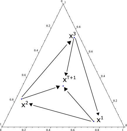
Figure 1: WGARP is satisfied but GARP fails

As for item (iii), the question about counterfactual bounds on demand turns out to have a simple answer. In fact, the answers for WGARP and GARP are analogous. We can build counterfactual bounds for demand consistent with WGARP with a direct modification of the approach by Varian (1982). Evidently, WGARP is a weaker condition than GARP, and provides less informative bounds to demand for a new price. At the same time, such bounds are easier to compute, and possibly more robust, in that they require only local consistency. We provide Afriat-like inequalities for WGARP that facilitate testing this condition using modern linear/integer programming techniques. These inequalities seem to be new to the literature.

In contrast to item (iii), item (iv) –i.e., the question concerning shape constraints on the preference function– has an answer that is remarkably different from the classical work by Afriat (1967) and Varian (1982). In fact, we observe that convexity of preferences is a testable shape constraint in finite data sets: there are data sets satisfying WGARP that cannot be rationalized by preference functions that are quasiconcave in the first argument. This means that these data sets cannot be rationalized by convex preferences. This finding provides a counterexample to Samuelson’s eternal darkness, which refers to the impossibility of testing convexity of preferences in the case of utility maximization. (Incidentally, the lack of convexity of some preference functions is precisely the reason that recovering preferences can no longer use the tools in Varian (1982).) Congruent with our analysis, John (2001) provides necessary and sufficient conditions for quasiconcavity of the preference function. And following Brown and Calsamiglia 2007; Allen and Rehbeck 2018, we next focus on the study of a quasilinear restriction on the local utilities in the maximin preference function representation, and show in Theorem 4 that this restriction is associated with the law of demand. This characterization may be of interest in its own right, due to the importance of the law of demand in both theoretical and applied literatures.

The direct predecessors of our work are the contributions of Kim and Richter (1986) and Quah (2006). Both works provide rationalizations of demand correspondences (or functions) consistent with WGARP (or WARP) with additional conditions on the invertibility of demand. The current work generalizes their results in two respects: (i) it provides a rationalization of WGARP/WARP for finite data sets, and (ii) for the case of infinite data sets, it relaxes a key invertibility assumption in both papers, i.e., we do not require that the set of prices at which any commodity bundle be chosen is nonempty.

This paper’s findings should be helpful for practitioners of revealed preferences since, from an empirical perspective, WGARP is significantly easier to work with than Varian’s GARP. In applications, it is common for practitioners to use WGARP as a synonymous of GARP. However, this is only true if price variation is limited, as shown in Cherchye et al. (2018). For example, it may happen that a finite data set of prices and observed consumption choices is consistent with WGARP, but cannot be rationalized by a utility function. If this occurs, the interpretation of the direct revealed-preference relation is unclear, yet we show that meaningful welfare analysis is possible.

The plan of the paper is as follows. After the central notions of revealed-preference theory are reviewed in section 2, sections 3 to 6 deal in turn with the questions posed on items (i) to (iv) discussed above. Section 7 extends the analysis to infinite data sets. Section 8 is a brief review of related literature, and section 9 concludes. Proofs are collected in an appendix.

2.  Preliminaries

Suppose that a consumer chooses bundles consisting of $L\geq 2$ goods in a market. We assume that we have access to a finite number of observations, denoted by $T$, on the prices and chosen quantities of these goods, where observations are indexed by $\mathbb{T=}\left\{1,\ldots,T\right\}$. Let $x^{t}\in X\equiv\mathbb{R}_{+}^{L}\setminus\{0\}$ denote the bundle of goods at time $t\in\mathbb{T}$, which was bought at prices $p^{t}\in P\equiv\mathbb{R}_{++}^{L}$. We impose Walras’ law throughout: wealth at time $t$ is equivalent to $p^{t}x^{t}\in W\equiv\mathbb{R}_{++}$, for all $t\in\mathbb{T}$. We write $O^{T}=\{p^{t},x^{t}\}_{t\in\mathbb{T}}$ to denote all price-quantity observations, and refer to $O^{T}$ as the data. In practice, the data $O^{T}$ describe a single consumer that is observed over time.

2.1. Revealed-Preference Axioms

We begin by recalling some key definitions in the revealed-preference literature.

Definition 1.

(Direct revealed preferred relations) We say that $x^{t}$ is directly revealed preferred to $x^{s}$, written $x^{t}\succeq^{R,D}x^{s}$, when $p^{t}x^{t}\geq p^{t}x^{s}$. Also, $x^{t}$ is strictly and directly revealed preferred to $x^{s}$, written $x^{t}\succ^{R,D}x^{s}$, when $p^{t}x^{t}>p^{t}x^{s}$.

If $x^{t}$ is directly revealed preferred to $x^{s}$, this means that the consumer chose $x^{t}$ and not $x^{s}$, when both bundles were affordable. If $x^{t}$ is strictly and directly revealed preferred to $x^{s}$, then she could also have saved money by choosing $x^{s}$. These definitions only compare pairs of bundles. We can extend them to compare any subset of bundles by using the transitive closure of the direct relation:

Definition 2.

(Revealed preferred relations) We say that $x^{t}$ is revealed preferred to $x^{s}$, written $x^{t}\succeq^{R}x^{s}$, when there is a chain $(x^{1},x^{2},\ldots,x^{n})\in\mathbb{T}$ with $x^{1}=x^{t}$ and $x^{n}=x^{s}$ such that $x^{1}\succeq^{R,D}x^{2}\succeq^{R,D}\ldots\succeq^{R,D}x^{n}$. Also, $x^{t}$ is strictly revealed preferred to $x^{s}$, written $x^{t}\succ^{R}x^{s}$, when at least one of the directly revealed relations in the revealed preferred chain is strict.

Hence, the revealed preferred relation $\succeq^{R}$ is the transitive closure of the direct revealed-preference relation $\succeq^{R,D}$. Next, we use these binary relations to define axioms that characterize different types of rational consumer behavior. We begin with Samuelson’s (1938) weak axiom of revealed preference:

Axiom 1.

(WARP) The weak axiom of revealed preference (WARP) holds if there is no pair of observations $s,t\in\mathbb{T}$ such that $x^{t}\succeq^{R,D}x^{s}$, and $x^{s}\succeq^{R,D}x^{t}$, with $x^{t}\neq x^{s}$.

Kihlstrom et al. (1976) introduces a generalized version of WARP:

Axiom 2.

(WGARP) The weak generalized axiom of revealed preference (WGARP) holds if there is no pair of observations $s,t\in\mathbb{T}$ such that $x^{t}\succeq^{R,D}x^{s}$, and $x^{s}\succ^{R,D}x^{t}$.

Samuelson (1948) shows how WARP can be used to construct a set of indifference curves in the two-dimensional ($L=2$) case, but also recognizes that WARP is not enough to characterize rationality in the multi-dimensional ($L>2$) case. Responding to this challenge, Houthakker (1950) introduces the strong axiom of revealed preference (SARP), which makes use of transitive comparisons between bundles as implied by the revealed preferred relation:

Axiom 3.

(SARP) The strong axiom of revealed preference (SARP) holds if there is no pair of observations $s,t\in\mathbb{T}$ such that $x^{t}\succeq^{R}x^{s}$, and $x^{s}\succeq^{R,D}x^{t}$, with $x^{t}\neq x^{s}$.

Varian (1982) notes that SARP requires single-valued demand functions, and argues that it is empirically more convenient to work with demand correspondences and “flat” indifference curves. To accomodate these properties, Varian introduces the generalized axiom of revealed preference (GARP):

Axiom 4.

(GARP) The generalized axiom of revealed preference (GARP) holds if there is no pair of observations $s,t\in\mathbb{T}$ such that $x^{t}\succeq^{R}x^{s}$ and $x^{s}\succ^{R,D}x^{t}$.

In the two-dimensional ($L=2$) case, the following equivalences are known:

Theorem A. (Equivalence of axioms) Let $L=2$. Consider a finite data set $O^{T}=\{p^{t},x^{t}\}_{t\in\mathbb{T}}$:

• The data $O^{T}$ satisfies SARP if and only if $O^{T}$ satisfies WARP (Rose 1958).

• The data $O^{T}$ satisfies GARP if and only if $O^{T}$ satisfies WGARP (Banerjee and Murphy 2006).

2.2. Revealed-Preference Characterizations

In this section, we recall the main results from the revealed-preference literature that are needed in order to introduce our contribution. Consider the following definitions of rationalization:

Definition 3.

(Utility rationalization) Consider a data set $O^{T}=\{p^{t},x^{t}\}_{t\in\mathbb{T}}$ and a utility function $u:X\mapsto\mathbb{R}$. For all $x\in X$ and all $t\in\mathbb{T}$ such that $p^{t}x\leq p^{t}x^{t}$,

• the data $O^{T}$ is weakly rationalized by $u$ if $u(x^{t})\geq u(x)$.

• the data $O^{T}$ is strictly rationalized by $u$ if $u(x^{t})>u(x)$ whenever $x\neq x^{t}$.

Afriat’s (1967) fundamental theorem is well known:

Theorem B. (Afriat’s theorem, Varian 1982) Consider a finite data set $O^{T}=\{p^{t},x^{t}\}_{t\in\mathbb{T}}$. The following statements are equivalent:

1. The data $O^{T}$ can be weakly rationalized by a locally nonsatiated utility function.

2. The data $O^{T}$ satisfies GARP.

3. There exist numbers $U^{t}$ and $\lambda^{t}>0$ for all $t\in\mathbb{T}$ such that the Afriat inequalities:

   $$U^{t}-U^{s}\geq\lambda^{t}p^{t}(x^{t}-x^{s}),$$

   hold for all $s,t\in\mathbb{T}$.

4. There exist numbers $V^{t}$ for all $t\in\mathbb{T}$ such that the Varian inequalities:

   $$\text{if }p^{t}(x^{t}-x^{s}) \geq 0\text{ then, }V^{t}-V^{s}\geq 0,$$

   $$\text{if }p^{t}(x^{t}-x^{s}) > 0\text{ then, }V^{t}-V^{s}>0,$$

   hold for all $s,t\in\mathbb{T}$.

5. The data $O^{T}$ can be weakly rationalized by a continuous, strictly increasing, and concave utility function.

There are several interesting features of Afriat’s theorem. Statements (ii), (iii), and (iv) give testable conditions that are easy to implement in practice (See, e.g., Demuynck and Hjertstrand 2019). Perhaps the most interesting theoretical implication of Afriat’s theorem is that statements (i) and (v) are equivalent, which means that continuity, monotonicity, and concavity are nontestable properties. In other words, separate violations of any of these properties cannot be detected in finite data sets.

Varian (1982) shows that the numbers $U^{t}$ and $\lambda^{t}$ in statement (iii) can be interpreted as measures of the utility level and marginal utility level of income at observation $t\in\mathbb{T}$. Analogously, Demuynck and Hjertstrand (2019) shows that the numbers $V^{t}$ in statement (iv) can be interpreted as measures of the utility levels at the observed demands.

Matzkin and Richter (1991) provides an analogous result for strict rationalization, by showing that SARP is a necessary and sufficient condition for a data set $O^{T}$ to be strictly rationalized by a continuous, strictly increasing, and strictly concave utility function:

Theorem C. (Matzkin and Richter 1991) Consider a finite data set $O^{T}=\{p^{t},x^{t}\}_{t\in\mathbb{T}}$. The following statements are equivalent:

1. The data $O^{T}$ can be strictly rationalized by a locally nonsatiated utility function.

2. The data $O^{T}$ satisfies SARP.

3. There exist numbers $U^{t}$ and $\lambda^{t}>0$ for all $t\in\mathbb{T}$ such that the inequalities

   $$\text{if }x^{t} \neq x^{s}\text{ then, }U^{t}-U^{s}>\lambda^{t}p^{t}\left(x^{t}-x^{s}\right),$$

   $$\text{if }x^{t} = x^{s}\text{ then, }U^{t}-U^{s}=0,$$

   hold for all $s,t\in\mathbb{T}$.

4. There exist numbers $V^{t}$ for all $t\in\mathbb{T}$ such that the inequalities:

   $$\text{if }x^{t} \neq x^{s}\text{ and }p^{t}(x^{t}-x^{s})\geq 0\text{ then, }V^{t}-V^{s}>0,$$

   $$\text{if }x^{t} = x^{s}\text{ then, }V^{t}-V^{s}=0,$$

   hold for all $s,t\in\mathbb{T}$.

5. The data $O^{T}$ can be strictly rationalized by a continuous, strictly increasing and strictly concave utility function.

Matzkin and Richter’s (1991) theorem mirrors Afriat’s, in the sense that it shows that continuity, monotonicity, and strict concavity are nontestable properties. Although much is known about the types of consumer behavior that characterize finite data sets satisfying SARP and GARP, there are no analogous characterizations for WARP and WGARP. The current paper, starting with the next section, fills this gap.

3.  Characterizations of WGARP and WARP

In this section, we provide revealed-preference characterizations, analogous to the ones in Afriat’s and Matzkin and Richter’s theorems, for WGARP and WARP. We begin by introducing the maximin preference model, which, to the best of our knowledge, is a new model of consumer behavior.

3.1. The Maximin Preference Model

We start with some preliminaries.

Definition 4.

(Preference function) A preference function is a mapping $r:X\times X\to\mathbb{R}$, that maps ordered pairs of commodity bundles to real numbers.

A preference function is a numerical representation of a consumer’s preferences. If $r(x,y)\geq 0$ then the consumer prefers bundle $x$ to $y$. Similarly, if $r(x,y)>0$, we say that $x$ is strictly preferred to $y$.

In what follows, we focus on a particular representation of $r$, namely the maximin model. Let $U$ be a finite index set that enumerates a collection of reference points. We define a reference point as a pair of observations, consisting of two price vectors and the corresponding vectors of commodity bundles $((p^{i},x^{i}),(p^{j},x^{j}))\in(P\times X)^{2}$ for $i,j\in U$. We consider a collection of reference-dependent utility functions $u_{ij}:X\to\mathbb{R}$, with the property that if $p^{i}x^{i}\geq(>)p^{i}y$ for all $y\in X$, then it must be the case that $u_{ij}(x^{i})\geq(>)u_{ij}(y)$, for all $i,j\in U$. We assume that the reference-dependent utility functions are independent of permutations of the indices in the subscript, so that $u_{ij}=u_{ji}$ for all $i,j\in U$. Let $\Delta(U)$ be the probability simplex defined on $U$.

Definition 5.

(Maximin (strict) preference model) We say that the preference function $r(x,y)$ is a maximin (strict) preference function if, for any $x,y\in X$, it can be written as:

$$r(x,y) =\max_{\mu\in\Delta(U)}\min_{\lambda\in\Delta(U)}\sum_{i\in U}\sum_{j\in U}\lambda_{i}\mu_{j}(u_{ij}(x)-u_{ij}(y)),$$

where, for any reference point indexed by $i,j\in U$, the ’local’ utility function, $u_{ij}$, is continuous, strictly increasing, and (strictly) concave.

The maximin preference function assigns a numerical value to the comparison of any pair of commodity bundles $x,y\in X$, by aggregating over local preferences that are defined for any reference point in the set $U$. More specifically, the aggregation is a maximin function, which in the first dimension takes the maximal difference between the utility gains of $x$ over $y$, and in the second dimension, takes the minimal value of that difference, over the different ’local’ utility functions.

The maximin aggregation structure is appealing because the preference function effectively extends the incomplete direct revealed preference relation when it is asymmetric (i.e., when WGARP holds) to the commodity space $X$. As such, this representation provides us with an interpretation of the direct revealed preference relation when rationality –GARP– fails, but WGARP is satisfied.

For any reference point indexed by $i,j\in U$, the local utility function, $u_{ij}$, is continuous, strictly increasing, and (strictly) concave. Moreover, the maximin is achieved at a particular reference point. Thus, for any pairwise comparison, a consumer behaves as if they are rational. However, note from the definition of $u_{ij}$ that, for any distinct pairwise comparison that is not a permutation, the preferences may change, in which case, preferences are not stable across all observations. In the maximin (strict) preference model, a consumer still behaves locally “as if she were rational” in that behavior according to this model rules out binary inconsistencies. More precisely, we show that a data set $O^{T}$ satisfies (WARP) WGARP if and only if the maximin (strict) preference model (strictly) rationalizes the data.

As a special case, when all local utility functions are the same, i.e., $u_{ij}=u$ for all $i,j\in U$, the maximin preference model reduces to standard utility maximization. Then, $r(x,y)=u(x)-u(y)$ for all $x,y\in X$. As such, traditional utility maximization is a case of global rationality, as opposed to the new notion of local rationality introduced here.

Next, we present some properties of the preference function. We begin with a property that turns out to be key in our characterizations of WARP and WGARP:

Definition 6.

(Skew-symmetry) We say that a preference function $r:X\times X\mapsto\mathbb{R}$ is skew-symmetric if $r(x,y)=-r(y,x)$ for all $x,y\in X$.

Skew-symmetry means that the preference function $r$ induces a preference order on $X$ that is complete and asymmetric. Note that, when a data $O^{T}$ satisfies WGARP, then the direct preference relation is an (incomplete) asymmetric relation on $X$, the preference function $r$ extends it if it is a maximin function. We have the following result:

Lemma 1.

If $r$ is a maximin preference function, then for any $x,y\in X$, we have:

$$r(x,y) =\max_{\mu\in\Delta(U)}\min_{\lambda\in\Delta(U)}\sum_{i\in U}\sum_{j\in U}\lambda_{i}\mu_{j}(u_{ij}(x)-u_{ij}(y))$$

$$=\min_{\lambda\in\Delta(U)}\max_{\mu\in\Delta(U)}\sum_{i\in U}\sum_{j\in U}\lambda_{i}\mu_{j}(u_{ij}(x)-u_{ij}(y)),$$

and moreover, $r$ is skew-symmetric.

The proof of this lemma is omitted, as it follows directly from the classical von Neumann’s minimax theorem. It is easy to see that the maximin preference function is skew-symmetric, making this model a variant of the general nontransitive consumer model, considered in Shafer (1974).

The next definition lists some additional important properties of preference functions, which will connect with the maximin preference model in the following section:

Definition 7.

Consider a preference function $r:X\times X\rightarrow\mathbb{R}$. We say that:

1. $r$ is continuous if for all $y\in X$ and any sequence $\left\{x^{n}\right\}$ of elements in $X$ that converges to $x\in X$ it must be that $\lim_{n\rightarrow\infty}r\left(x^{n},y\right)=r\left(x,y\right)$.

2. $r$ is locally nonsatiated if for any $x,y\in X$ such that $r\left(x,y\right)=0$ and for any $\epsilon>0$, there exists a $y^{\prime}\in B(y,\epsilon)$ such that $r\left(x,y^{\prime}\right)<0$.

3. $r$ is strictly increasing if for all $x,y,z\in X$, $x\geq z$ implies $r(x,y)>r(z,y)$.

4. $r$ is quasiconcave if for all $x,y,z\in X$ and any $0\leq\lambda\leq 1$ we have $r\left(x^{\lambda},y\right)\geq\min\left\{r\left(x,y\right),r\left(z,y\right)\right\}$, where $x^{\lambda}=\lambda x+\left(1-\lambda\right)z$, and strictly quasiconcave if, for any $0<\lambda<1$, the inequality is strict whenever $x\neq z$.

5. $r$ is concave if for all $x,y,z\in X$ and any $0\leq\lambda\leq 1$ we have $r\left(x^{\lambda},y\right)\geq\lambda r\left(x,y\right)+\left(1-\lambda\right)r\left(z,y\right)$, and strictly concave if, for any $0<\lambda<1$, the inequality is strict whenever $x\neq z$.

6. $r$ is piecewise concave if there is a sequence of concave functions in the first argument $f_{t}\left(x,y\right)$ for $t\in\mathbb{K}$ in a compact set such that $r\left(x,y\right)=\max_{t\in\mathbb{K}}\left\{f_{t}\left(x,y\right)\right\}$, and strictly piecewise concave if there is a similar sequence of strictly concave functions.

Some remarks are in order: Continuity is a technical condition that is convenient to ensure existence of a maximum in the constrained maximization of the preference function. Local nonsatiation rules out thick indifference curves: if we take an arbitrarily small neighborhood of a bundle that is indifferent to a given bundle $x$, the neighborhood contains bundles that are dominated by $x$. Strict monotonicity simply means that "more is better". Quasiconcavity says that for a fixed reference point $y\in X$, a mixture of two bundles $x,z\in X$ is at least as good as the worst of the two bundles, according to the preference function. Concavity is a cardinal version of quasiconcavity. Quasiconcavity and concavity are important properties because they ensure well-behaved optimization problems. More precisely, quasiconcavity guarantees that a function defined on a compact set has a convex set of maxima points, while a strictly concave function defined on a compact set always has a unique global maximum.

Piecewise concavity and its strict version are new properties, which turn out to be especially important for our characterizations of WGARP/WARP. The property says that for a fixed $y\in X$, a mixture of two bundles $x,z\in X$ is at least as good as the worst one of the two bundles, but only if $x,z$ are close enough. In other words, this is a local version of concavity, implying local quasiconcavity.

3.2. Preference Function Rationalization

We now introduce the notion of (strict) rationalization by a preference function, which is analogous to utility rationalization in Definition 3:

Definition 8.

(Preference function rationalization) Consider a data set $O^{T}=\{p^{t},x^{t}\}_{t\in\mathbb{T}}$ and a preference function $r:X\times X\mapsto\mathbb{R}$. For all $x\in X$ and all $t\in\mathbb{T}$ such that $p^{t}x\leq p^{t}x^{t}$,

• the data $O^{T}$ is weakly rationalized by $r$ if $r(x^{t},x)\geq 0$.

• the data $O^{T}$ is strictly rationalized by $r$ if $r(x^{t},x)>0$ whenever $x\neq x^{t}$.

The next definition introduces the concept of rationalization in terms of the maximin preference model:

Definition 9.

(Maximin preference rationalization) The data $O^{T}$ is weakly (strictly) rationalized by a maximin (strict maximin) preference function $r$ if $r$ is a maximin (strict maximin) preference function as stated in Definition 5, and $O^{T}$ is weakly (strictly) rationalized by $r$ as stated in Definition 8.

In the subsequent two sections, we show that WGARP (WARP) is a necessary and sufficient condition for a data set $O^{T}$ to be rationalized by the maximin (strict maximin) preference model.

3.3. WGARP

The next theorem provides a revealed-preference characterization of WGARP for finite data sets. This result mirrors Afriat’s theorem in terms of preference function rationalization (as opposed to utility rationalization):

Theorem 1.

Consider a finite data set $O^{T}=\{p^{t},x^{t}\}_{t\in\mathbb{T}}$. The following statements are equivalent:

1. The data $O^{T}$ can be weakly rationalized by a locally nonsatiated and skew-symmetric preference function.

2. The data $O^{T}$ satisfies WGARP.

3. There exist numbers $R^{t,s}$ and $\lambda_{ts}^{t}>0$ for all $s,t\in\mathbb{T}$ with $R^{t,s}=-R^{s,t}$ and $\lambda_{ts}^{t}=\lambda_{st}^{t}$ such that inequalities:

   $$R^{t,s}\geq\lambda_{ts}^{t}p^{t}(x^{t}-x^{s}),$$

   hold for all $s,t\in\mathbb{T}$.

4. There exist numbers $W^{t,s}$ for all $s,t\in\mathbb{T}$ with $W^{t,s}=-W^{s,t}$ such that inequalities:

   $$\text{if }p^{t}(x^{t}-x^{s})\geq 0\text{ then, }W^{t,s}\geq 0,$$

   $$\text{if }p^{t}(x^{t}-x^{s})>0\text{ then, }W^{t,s}>0,$$

   hold for all $s,t\in\mathbb{T}$.

5. The data $O^{T}$ can be weakly rationalized by a maximin preference function.

6. The data $O^{T}$ can be weakly rationalized by a continuous, strictly increasing, piecewise concave, and skew-symmetric preference function.

The equivalence of statements (i) and (vi) shows that, if the data can be weakly rationalized by any nontrivial preference function at all, it can, in fact, be weakly rationalized by a preference function that satisfies continuity, monotonicity, and piecewise concavity. Put differently, separate violations of these three properties cannot be detected in finite data sets.

The numbers $R^{t,s}$ and $\lambda^{t}_{st}$ in statement (iii) have a similar interpretation as in Afriat’s theorem for each reference point; that is, if we consider $t,s\in\mathbb{T}$, then $R^{t,s}$ is a measure of the utility difference $u_{ts}(x^{t})-u_{ts}(x^{s})$ for that particular pairwise data set, while $\lambda^{t}_{st}$ is a measure of the marginal utility level of income at observation $t\in\mathbb{T}$ for the pairwise data set.

3.4. WARP

The next theorem provides a revealed-preference characterization of WARP for finite data sets, and mirrors Matzkin and Richter’s (1991) theorem:

Theorem 2.

Consider a finite data set $O^{T}=\{p^{t},x^{t}\}_{t\in\mathbb{T}}$. The following statements are equivalent:

1. The data $O^{T}$ can be strictly rationalized by a locally nonsatiated and skew-symmetric preference function.

2. The data $O^{T}$ satisfies WARP.

3. There exist numbers $R^{t,s}$ and $\lambda_{ts}^{t}>0$ for all $s,t\in\mathbb{T}$ with $R^{t,s}=-R^{s,t}$ and $\lambda_{ts}^{t}=\lambda_{st}^{t}$ such that inequalities:

   $$\text{if }x^{t} \neq x^{s}\text{ then, }R^{t,s}>\lambda_{ts}^{t}p^{t}\left(x^{t}-x^{s}\right),$$

   $$\text{if }x^{t} = x^{s}\text{ then, }R^{t,s}=0,$$

   hold for all $s,t\in\mathbb{T}$.

4. There exist numbers $W^{t,s}$ for all $s,t\in\mathbb{T}$ with $W^{t,s}=-W^{s,t}$ such that inequalities:

   $$\text{if }x^{t} \neq x^{s}\text{ and }p^{t}(x^{t}-x^{s})\geq 0\text{ then, }W^{t,s}>0,$$

   $$\text{if }x^{t} = x^{s}\text{ then, }W^{t,s}=0,$$

   hold for all $s,t\in\mathbb{T}$.

5. The data $O^{T}$ can be strictly rationalized by a maximin strict preference function.

6. The data $O^{T}$ can be strictly rationalized by a continuous, strictly increasing, piecewise strictly concave, and skew-symmetric preference function.

Analogous to Theorem 1, this result shows that separate violations of continuity, monotonicity, and strict piecewise concavity cannot be detected in finite data sets.

4.  Recoverability of Preferences

In this section, we tackle the question of when one can use the direct revealed-preference relation elicited from the observed consumer behavior in order to make inferences about her true preferences. We begin by showing that recovering preferences using WGARP does not follow as a trivial corollary of the original approach proposed by Varian (1982). We next propose an alternative method to recover bounds of preferences using WGARP.

4.1. Varian’s Approach to Recover Bounds on Preferences Using WGARP

At this point, it is useful to briefly recall the classical approach from Varian (1982), which finds upper and lower bounds to the true preferences of a consumer. The object of interest is the true preference of the consumer, captured by the strict upper contour set of a commodity bundle $x$ according to the true preference function $r$:

Definition 10.

(Set of strictly better alternatives) We define the set of strictly better alternatives than a (possibly unobserved) commodity bundle $x\in X$ as:

$$U_{r}(x)=\{y\in X:r(y,x)>0\},$$

for the true preference function $r$.

Varian (1982) defines the supporting set of prices for any new commodity bundle $x\in X$ so that the extended data set, $O^{T}\cup\{p,x\}$, satisfies GARP as:

$$S(x)=\{p\in P:O^{T}\cup\{p,x\}\text{\>satisfies GARP}\}.$$

Varian then uses the set $S(x)$ to create upper and lower bounds for the set of interest $U_{r}(x)$. We need to define two new sets. The revealed worse set is

$$RW(x)=\{y\in X:\forall p\in S(x),x\succ^{{R,D}}_{O^{T}\cup\{(p,x)\}}y\}$$

for $\succ^{R,D}$, defined on the extended data set $O^{T}\cup\{(p,x)\}$. The nonrevealed worse set $NRW(x)$ is the complement of $RW(x)$. The revealed preferred set is

$$RP(x)=\{y\in X:\forall p\in S(y),y\succ^{R,D}_{O^{T}\cup\{(p,y)\}}x\}.$$

Varian (1982) shows that, in the case of utility maximization (i.e., $r(x,y)=u(x)-u(y)$), for some $u:X\to\mathbb{R}$ and all $x,y\in X$) we have:

$$RP(x)\subseteq U_{r}(x)\subseteq NRW(x).$$

One would be tempted to use the same construction for WGARP by replacing the definition of the supporting set $S(x)$ with one where the extended data set satisfies WGARP. Of course, when the data consists of two goods (i.e., $L=2$), this does not cause any problems since, in such a case, WGARP and GARP are equivalent (See Theorem A). However, if $L>2$, as we show, performing such an exercise is generally not advisable. In particular, we illustrate this by means of an example that, in some cases, yields an uninformative upper bound set $NRW(x)$.

We begin the elaboration of these points by using an example in Keiding and Tvede (2013):

Example 1.

(Keiding and Tvede 2013, Example 1, p.467) Consider a data set $O^{3}$ with prices $p^{1}=(4\>1\>5)^{\prime}$, $p^{2}=(5\>4\>1)^{\prime}$, $p^{3}=(1\>5\>4)^{\prime}$, and bundles $x^{1}=(4\>1\>1)^{\prime}$, $x^{2}=(1\>4\>1)^{\prime}$, $x^{3}=(1\>1\>4)^{\prime}$. It is easy to verify that this data set satisfies WGARP. The objective is to recover the preferences of this consumer for a new commodity bundle, $x^{T+1}$, given this observed behavior. Suppose that the unobserved commodity bundle is:

$$x^{T+1}=\frac{1}{3}(x^{1}+x^{2}+x^{3})=(2\>2\>2)^{\prime}.$$

If the analyst were to use the methods in Varian (1982), she would need to recover all prices $p^{T+1}$ for which the extended data set $O^{3}\cup(p^{T+1},x^{T+1})$ satisfies WGARP. In this extended data set, we have $p^{t}(x^{t}-x^{T+1})=2>0$, for all $t=1,2,3$. However, there is no $p\in P$ for which $p(x^{T+1}-x^{t})<0$, for all $t=1,2,3$. This implies that this extended data set fails WGARP. This presents a problem, if we want to recover preferences using Varian’s (1982) approach, because it implicitly assumes that the analyst can always find at least one such vector of prices.

In this example, Varian’s supporting set is empty, i.e., $S(x^{T+1})=\emptyset$. Moreover, it directly follows that any monotonically dominated bundle such as $x^{-}=(1\>1\>1)$ cannot be ruled out from the set $U_{r}(x)$. Consequently, the upper bound of $U_{r}(x^{T+1})$ is uninformative, i.e., $NRW(x^{T+1})=X\setminus{x^{T+1}}$. Thus, any analysis based on this approach is problematic, since the data set $O^{3}$ can be rationalized by a preference function that is strictly increasing (in the first argument). In other words, Varian’s method to bound preferences does not yield any valuable information in this example.

Yet the method proposed by Varian (1982) to recover preferences for GARP is often useful. Our analysis simply says that recoverability of preferences in terms of WGARP does not follow as a trivial corollary of Varian’s results. We can also clarify the source of this failure. Consider Example 1 again, and note that the original data satisfies WGARP, which implies that there is a preference function $r$ that rationalizes the data. Moreover, we have that $r(x_{1},x_{2})>0$, $r(x_{2},x_{3})>0$, and $r(x_{3},x_{1})>0$. In addition, we know that the new bundle, $x^{T+1}$, is a convex combination of the observed bundles. Given the equivalence between GARP and convexity of preferences, if we followed Varian’s approach then we would be implicitly assuming that preferences are convex. But, in our case, convexity of preferences is implied by the assumption that the preference function is quasiconcave in its first argument, in which case, we must have $r(x^{T+1},x^{T+1})=0\geq\min_{t=1,2,3}\{r(x^{t},x^{T+1})\}$. This implies that $x^{T+1}$ must be revealed to be weakly better than at least one of the three observed bundles $x^{1},x^{2}$, and $x^{3}$. However, note that, for all $t=1,2,3$, we have $p^{t}(x^{t}-x^{T+1})=2>0$. This implies that, if the consumer is maximizing a quasiconcave preference function, then all observed commodity bundles must be strictly preferred to the new bundle, i.e., $r(x^{t},x^{T+1})>0$ for all $t=1,2,3$. Hence, the extended data set $O^{3}\cup\{p,x^{T+1}\}$ cannot be weakly rationalized by a quasiconcave and skew-symmetric preference function.

Interestingly, this example also shows that quasiconcavity of the preference function is, in fact, a testable property in finite data sets. As such, this is also a counterexample to Samuelson’s eternal darkness conjecture, that any finite data set always can be rationalized by a convex preference relation. Summarizing these results, the lack of convexity of preferences, which can be inferred from behavior consistent with WGARP, limits the applicability of the tools developed in the classical treatment by Varian (1982). In section 6.1, we will return to the study of the testable implications of convexity.

4.2. A New Approach to Recover Bounds on Preferences Using WGARP

In this subsection, we use the new notion of maximin preference rationalization as a way to provide new informative bounds of the true preferences. We show that these new bounds escape the problems associated with Varian’s approach.

We have shown, in the proof of Theorem 1, that, without loss of generality, we can identify the index set of reference point situations $U$ with the set of observations $\mathbb{T}$, so that we have a local true utility $u_{s,t}$ for all $s,t\in\mathbb{T}$, in which case the true global preferences for any $x^{\prime},x\in X$ are given by:

$$r(x^{\prime},x)=\max_{\mu\in\Delta(\mathbb{T})}\min_{\lambda\in\Delta(\mathbb{T})}\sum_{t\in\mathbb{T}}\sum_{s\in\mathbb{T}}\lambda_{s}\mu_{t}(u_{st}(x^{\prime})-u_{st}(x)).$$

We have also shown that any data set $O^{T}$ satisfying WGARP can be broken into $T^{2}$ pairwise data sets $O^{2}_{st}=\{(p^{t},x^{t}),(p^{s},x^{s})\}$, and have argued that each one of these data sets satisfies GARP. Define the ’local’ (Varian) support set as $S_{st}(x)$ for any $x\in X$. For a data set of $T$ observations, note that we have a collection of $T^{2}$ such ’local’ support sets, and that everyone of these sets is never empty:

Definition 11.

(WGARP-robust revealed preferred set) For each $s,t\in\mathbb{T}$ let

$$RP_{st}(x)=\{y\in X:\forall p\in S_{st}(y),py>px\}$$

be the pairwise revealed preferred set. We define the (WGARP-)robust revealed preferred set as:

$$RP^{W}(x)=\cup_{s\in\mathbb{T}}\cap_{t\in\mathbb{T}}RP_{st}(x).$$

Next, we argue that the robust revealed preferred set is a lower bound of $U_{r}(x)$ for all $x\in X$. If $x^{\prime}\in RP^{W}(x)$, this implies that $x^{\prime}\in RP_{st}(x)$ for all $t\in\mathbb{T}$ and for some $s^{*}\in\mathbb{T}$. Thus, it must be the case that, for $s^{*}$ and for all $t\in\mathbb{T}$, $u_{s^{*}t}(x^{\prime})>u_{s^{*}t}(x)$. This means that $r(x^{\prime},x)\geq\min_{\mu}\sum_{t}\mu_{t}(u_{s^{*}t}(x^{\prime})-u_{s^{*}t}(x))>0$. Hence, we can conclude that, if $x^{\prime}\in RP^{W}(x)$, then $r(x^{\prime},x)>0$, which is the same as saying that $RP^{W}(x)\subseteq U_{r}(x)$.

Definition 12.

(WGARP-robust (non)revealed worse set) For each $s,t\in\mathbb{T}$, let

$$RW_{st}(x)=\{y\in X:\forall p\in S_{st}(x),px>py\}$$

be the pairwise revealed worse set. Let $NRW_{st}(x)$ be the complement of $RW_{st}(x)$. We define the (WGARP-)robust nonrevealed worse set as

$$NRW^{W}(x)=\cap_{s\in\mathbb{T}}\cup_{t\in\mathbb{T}}NRW_{st}(x).$$

From this definition, it directly follows that, if $r(x^{\prime},x)>0$, then $x^{\prime}\in NRW^{W}(x)$. To see this, note that, if $r(x^{\prime},x)>0$, then there must be some $t^{*}\in\mathbb{T}$ such that $u_{st^{*}}(x^{\prime})>u_{st^{*}}(x)$ for all $s\in\mathbb{T}$. This implies, by Varian 1982, that $x^{\prime}\in NRW_{st^{*}}(x)$ for all $s\in\mathbb{T}$. By Definition 12, we must have that $x^{\prime}\in NRW^{W}(x)$. Hence, we can conclude that $U_{r}(x)\subseteq NRW^{W}(x)$. The following theorem summarizes these results, confirming that the bounds recovered using Varian’s approach in this context are not sharp:

Theorem 3.

The upper contour set of the true preferences at any given $x\in X$ is:

$$RP^{W}(x)\subseteq U_{r}(x)\subseteq NRW^{W}(x).$$

Moreover, (i) the upper bound, $NRW(x)$, recovered using Varian’s approach is not sharp, i.e., $NRW^{W}(x)\subseteq NRW(x)$ for all $x\in X$ (with strict containment for some $x\in X$); and (ii) the lower bound, $RP(x)$, recovered using Varian’s approach is not sharp, i.e., $RP(x)\subseteq RP^{W}(x)$ for all $x\in X$ (with strict containment for some $x\in X$).

We note that, in the context of Example 1, $NRW^{W}(x^{T+1})$ does not contain the dominated commodity $x^{-}=(1\>1\>1)$. In fact, $NRW^{W}(x^{T+1})$ excludes all commodity bundles that are monotonically dominated by $x^{T+1}$, which is a desirable property, lacking in Varian’s analogous set $NRW(x^{T+1})=X\setminus{x^{T+1}}$. Similar statements can be made about the $RP^{W}(x^{-})$ set.

Theorem 3 has some important implications. The first part shows that the new method of using subsets of data sets for bound computation yields informative bounds. The second part highlights that a naive application of the methodology in Varian (1982), when the assumption of convex preferences does not hold, is problematic.

5.  Demand Counterfactuals

In this section, we show how to perform counterfactual analysis. That is, for a new (possibly unobserved) price vector $p^{T+1}$ we propose a simple method to provide a bound for the demanded bundle under WGARP. This method is a simplification of the procedure for the same purpose under GARP, proposed by Varian (1982).

Definition 13.

(W-Demand Set) We define the W-demand set, or the set of all commodity bundles compatible with WGARP, by

$$D(p^{T+1})=\{x\in X:O^{T}\cup\{p^{T+1},x\}\text{ satisfies WGARP and }p^{T+1}x=1\}.$$

The W-demand set for a new price-vector can be formulated as a linear program by making use of the following result:

Corollary 1.

The bundle $x^{T+1}\in X$ is in $D(p^{T+1})$ if and only if it satisfies:

1. $p^{T+1}x^{T+1}=1$,

2. $p^{t}x^{T+1}\geq p^{t}x^{t}$, for all $t\in\mathbb{T}$, for which $p^{T+1}x^{t}\leq p^{T+1}x^{T+1}$,

3. $p^{t}x^{T+1}>p^{t}x^{t}$, for all $t\in\mathbb{T}$, for which $p^{T+1}x^{t}<p^{T+1}x^{T+1}$.

The first condition is a normalization of wealth and imposes Walras’ law. The second condition imposes the restriction that, if the observed bundles are cheaper than the new bundle at the new prices, then the new bundle cannot be affordable at the observed prices. The third condition strengthens the second, for the case of a strict inequality. Note that, if the new bundle is cheaper at the new prices than the observed bundles, then the second and third conditions are redundant as WGARP is trivially satisfied for the extended data set.

Recently, Adams (2019) highlights some technical difficulties in the construction of the W-demand set, when predictions are made at more than a single price regime. For that case, Adams (2019) proposes a mixed integer linear programming (MILP) problem, which can be simplified for the case of WGARP using the results in Theorem 1. In particular, the inequalities in statement (iv) of Theorem 1 are useful for this purpose.

Cherchye et al. (2015) shows how the Varian inequalities in statement (iv) in Theorem B can be formulated as a MILP problem. This MILP problem can be modified in a straightforward way to check whether the inequalities in statement (iv) in Theorem 1 have a solution. Specifically, it follows from Theorem 4 in Cherchye et al. (2015) that statement (iv) in our Theorem 1 holds if and only if there exist numbers $R^{t,s}\in(-1,1)$, with $R^{t,s}=-R^{s,t}$, and binary variables $B^{t,s}\in\{0,1\}$ such that, for all observations $s,t\in\mathbb{T}$, the following linear inequalities (in $p$ and $x$) hold:

$$R^{t,s} <B^{t,s},$$

$$(B^{t,s}-1) \leq R^{t,s},$$

$$p^{t}(x^{t}-x^{s}) <B^{t,s}A^{t},$$

$$(B^{t,s}-1)A^{s} \leq p^{s}(x^{t}-x^{s}).$$

As a final remark, in contrast to recoverability of preferences for data sets consistent with WGARP, the construction of demand counterfactuals is just a simplification of the procedure outlined in Varian (1982). The main reason is that the construction of the W-demand set does not depend on duality arguments, which fail when quasiconcavity of the preference function does not hold.

6.  Shape Constraints: Concave Rationalization and the Law of Demand

We have shown, in sections 3.3 and 3.4, that WGARP (WARP) is a necessary and sufficient condition for a data set to be rationalized by a continuous, strictly increasing, skew-symmetric, and piecewise (strictly) concave preference function. In this section, we consider conditions that are necessary and sufficient for a data set to be rationalized under stronger shape restrictions.

6.1. Concave Rationalization

John (2001) provides conditions under which a data set can be weakly rationalized by a continuous, strictly increasing, skew-symmetric, and concave preference function:

Theorem D. (John 2001) Consider a data set $O^{T}=\{p^{t},x^{t}\}_{t\in\mathbb{T}}$. The following statements are equivalent:

1. The data $O^{T}$ can be weakly rationalized by a locally nonsatiated, concave, and skew-symmetric preference function.

2. There exist numbers $R^{t,s}$ and $\lambda^{t}>0$ for all $s,t\in\mathbb{T}$ with $R^{t,s}=-R^{s,t}$ such that the inequalities:

   $$R^{t,s}\geq\lambda^{t}p^{t}(x^{t}-x^{s}),$$

   hold for all $s,t\in\mathbb{T}$.

3. The data $O^{T}$ can be weakly rationalized by a continuous, strictly increasing, concave, and skew-symmetric preference function.

John (2001) provides additional testable conditions, which he shows are equivalent to condition (ii). By comparing John’s (2001) results with our Theorem 1, it is easy to see that his results imply any of the conditions in our theorem, but not vice versa. In particular, note that, in contrast to statement (iii) in Theorem 1, the indices $\lambda^{t}$ are constant across all pairs $s,t\in\mathbb{T}$. This ensures that John’s rationalizing preference function is indeed concave.

Of course, by Afriat’s theorem and the equivalence between WGARP and GARP (See Theorem A), concavity is a nontestable property when $L=2$. However, by Theorem 1 and Theorem D, when $L>2$, concavity is a testable property. This raises the question of whether it is at all possible to further strenghthen the results in Theorem 1, by showing that WGARP is equivalent to weak rationalization by means of a quasiconcave preference function. However, from the discussion in section 4.1, Example 1 shows that this is not the case. In fact, this is a counterexample showing that the data cannot be rationalized by a quasiconcave preference function. Thus, with a finite number of observations, Example 1 shows that quasiconcavity is a testable property.

6.2. The Law of Demand and Quasilinear Preference Functions

This subsection derives necessary and sufficient conditions for a data set to be rationalized by a continuous, strictly increasing, skew-symmetric, concave, and quasilinear preference function. Interestingly, we show that one such condition is the law of demand, and consequently, this is equivalent to rationalization by a maximin quasilinear preference function. Before presenting these results, we briefly recall the revealed-preference characterization for quasilinear-utility maximization.

6.2.a.  The Quasilinear Utility Maximization Model

First, we consider the definition of quasilinear utility maximization:

Definition 14.

(Quasilinear utility maximization) Consider a locally nonsatiated utility function $u(x)$. We say that a consumer facing prices $p\in P$ and income $w\in W$ is a quasilinear utility maximizer if she solves

$$\max_{x\in X}u(x)+w-px\iff\max_{x\in X,y\in\mathbb{R}}u(x)+y\>\>s.t.\>px+y\leq w.$$

As in standard applications of quasilinear utility maximization, we allow the numeraire $y$ to be negative in order to avoid technicalities related to corner solutions. Consider the following definition of quasilinear utility rationalization for a finite data set $O^{T}$:

Definition 15.

(Quasilinear utility rationalization) Consider a data set $O^{T}$ and a utility function $u:X\to\mathbb{R}$. For all $x\in X$, the data $O^{T}$ is rationalized by a locally nonsatiated and quasilinear utility function $u$ if, for all $t\in\mathbb{T}$:

$$u(x^{t})-p^{t}x^{t}\geq u(x)-p^{t}x.$$

Brown and Calsamiglia (2007) shows that the axiom of the strong law of demand is a necessary and sufficient condition for a data set to be rationalized by a continuous, strictly increasing, concave, and quasilinear utility function.

Axiom 5.

(Strong law of demand) The strong law of demand holds if, for all distinct choices of indices $(1,2,3,\ldots,n)\in\mathbb{T}$:

$$p^{1}(x^{1}-x^{2})+p^{2}(x^{2}-x^{3})+\cdots+p^{n}(x^{n}-x^{1})\leq 0.$$

The next theorem recalls the revealed-preference characterization of quasilinear utility maximization from Brown and Calsamiglia (2007) and Allen and Rehbeck (2018):

Theorem E. (Brown and Calsamiglia 2007; Allen and Rehbeck 2018) Consider a finite data set $O^{T}=\{p^{t},x^{t}\}_{t\in\mathbb{T}}$. The following statements are equivalent:

1. The data $O^{T}$ can be rationalized by a locally nonsatiated and quasilinear utility function.

2. The data $O^{T}$ satisfies the strong law of demand.

3. There exist numbers $U^{t}$ for all $t\in\mathbb{T}$ such that the inequalities:

   $$U^{t}-U^{s}\geq p^{t}(x^{t}-x^{s}),$$

   hold for all $s,t\in\mathbb{T}$.

4. The data $O^{T}$ can be rationalized by a continuous, strictly increasing, concave, and quasilinear utility function.

6.2.b.  The Law of Demand and the Quasilinear Preference Function Maximization Model

In this subsection, we provide analogous results for the quasilinear preference function model, and show that the law of demand is a necessary and sufficient condition for a data set to be rationalized by a continuous, strictly increasing, concave, skew-symmetric, and quasilinear preference function. The axiom of the law of demand is formally defined as:

Axiom 6.

(Law of demand) The law of demand holds if, for all observations $s,t\in\mathbb{T}$:

$$(p^{t}-p^{s})(x^{t}-x^{s})\leq 0.$$

For any sequence consisting of only two (distinct) observations $s,t\in\mathbb{T}$, it is easy to see that the strong law of demand and the law of demand are equivalent. Thus, in a sense, for the quasilinear model, the relation between the law of demand and the strong law of demand mirrors the relation between WGARP (WARP) and GARP (SARP). Before stating our revealed-preference characterization of the law of demand, we introduce the maximin quasilinear preference function, which is a particular representation of a quasilinear preference function:

Definition 16.

(Maximin quasilinear preference model) We say that the preference function $r(x,y)$ is a maximin quasilinear preference function if, for any $x,y\in X$, it can be written as:

$$r(x,y) =\max_{\mu\in\Delta(U)}\min_{\lambda\in\Delta(U)}\sum_{i\in U}\sum_{j\in U}\lambda_{i}\mu_{j}(u_{ij}(x)-u_{ij}(y)),$$

where, for any reference point indexed by $i,j\in U$, the ’local’ utility function $u_{i,j}$ is continuous, strictly increasing, concave, and quasilinear.

The next two definitions detail the notion of rationalization, in terms of the quasilinear preference function, and in the specific case of the maximin quasilinear preference function model:

Definition 17.

(Quasilinear preference function rationalization) Consider a data set $O^{T}$ and a preference function $r:X\times X\to\mathbb{R}$. For all $x\in X$ and all $t\in\mathbb{T}$, the data $O^{T}$ is rationalized by a locally nonsatiated and quasilinear preference function $r$ if

$$r(x^{t},x)-p^{t}(x^{t}-x)\geq 0.$$

Definition 18 (Maximin quasilinear preference rationalization).

The data $O^{T}$ is rationalized by a maximin quasilinear preference function $r$ if $r$ is a maximin quasilinear preference function as stated in Definition 16, and $O^{T}$ is rationalized by a locally nonsatiated and quasilinear preference function $r$ as stated in Definition 17.

The next theorem provides a revealed-preference characterization of the law of demand for finite data sets:

Theorem 4.

Consider a finite data set $O^{T}=\{p^{t},x^{t}\}_{t\in\mathbb{T}}$. The following statements are equivalent:

1. The data $O^{T}$ can be rationalized by a locally nonsatiated, skew-symmetric, and quasilinear preference function.

2. The data $O^{T}$ satisfies the law of demand.

3. There exist numbers $R^{t,s}$, for all $s,t\in\mathbb{T}$, with $R^{t,s}=-R^{s,t}$, such that inequalities:

   $$R^{t,s}\geq p^{t}(x^{t}-x^{s}),$$

   hold for all $s,t\in\mathbb{T}$.

4. The data $O^{T}$ can be rationalized by a maximin quasilinear preference function.

5. The data $O^{T}$ can be rationalized by a continuous, strictly increasing, concave, skew-symmetric, and quasilinear preference function.

7.  Infinite Data Sets: Characterizations of WGARP, WARP and the Law of Demand

Thus far, our results have been derived under the assumption that the researcher only observes a finite number of choices. In the original formulation of revealed-preference theory, Samuelson (1938) and Houthakker (1950) implicitly assume that the entire demand function, or a demand correspondence, is observed. In this section, we show that our main results from the previous sections can be transported to the case of infinite data sets, namely, when we observe a demand correspondence $\textbf{x}:P\times W\to 2^{X}\setminus{\emptyset}$, where $w\in W\equiv\mathbb{R}_{++}$ denotes wealth. We focus on compact sets of prices and consumption bundles, where, by abusing notation slightly, we denote $P\subset\mathbb{R}^{L}_{++}$ and $X\subset\mathbb{R}^{L}_{+}\setminus{0}$, as the sets of prices and consumption bundles, respectively. We continue to assume Walras’ law, so that $x\in\textbf{x}(p,w)$, $px=w$. We define the image of x as $\mathbf{X}=\cup_{p\in P,w\in W}\mathbf{x}(p,w)$. A central assumption throughout this section is that we can write the demand correspondence as a data set consisting of an infinite number of demand observations, which we denote by $O^{\infty}=\{p,x\}_{p\in P,x\in\textbf{X}:x\in\textbf{x}(p,px)}$.

7.1. WGARP and WARP

We begin by providing revealed-preference characterizations for WGARP and WARP. In doing so, we define the direct preference relations for infinite data sets as:

Definition 19.

(Direct Revealed Preferences) We say that $x\in\mathbf{X}$ is directly revealed preferred to $y\in\mathbf{X}$, written $x\succeq^{R,D}y$, when $px\geq py$ such that $x\in\mathbf{x}(p,px)$. Also, $x\in\mathbf{X}$ is directly revealed preferred to $y\in\mathbf{X}$, written $x\succ^{R,D}y$ when $px>py$ and $x\in\mathbf{x}(p,px)$.

Under this definition, the data $O^{\infty}$ satisfies WGARP if there is no pair $x,y\in\mathbf{X}$ such that $x\succeq^{R,D}y$ and $y\succ^{R,D}x$. Analogously, the data $O^{\infty}$ satisfies WARP if there is no pair $x,y\in\mathbf{X}$ such that $x\succeq^{R,D}y$ and $y\succeq^{R,D}x$.

We begin by generalizing the maximin rational preference function to the case of infinite data sets. For this, we need some preliminaries. For any reference point in the data set $O^{\infty}$, we rearrange the observations into a vector $o=(p^{\prime}\>a^{\prime}\>q^{\prime}\>b^{\prime})^{\prime}\in\mathbf{O}^{2}$, with $\mathbf{O}\subseteq P\times\mathbf{X}$ and $x\in\textbf{x}(p,px)$, such that each reference point can be thought as a column vector. In addition, we define $o_{1}=(p^{\prime}\>a^{\prime})^{\prime}$ and $o_{2}=(q^{\prime}\>b^{\prime})^{\prime}$, such that $o=(o_{1}^{\prime}\>o_{2}^{\prime})^{\prime}$.

We assume that the set of reference points O is compact, i.e., closed and bounded. There are several examples satisfying this condition; for instance, when there are a finite number of reference points, or when the demand correspondence that generates the data set is compact-valued. Hence, in the latter case, compactness of O follows from assuming that $\textbf{x}(p,px)$ is a compact set, which ensures that the entire set $P\times\mathbf{X}$ is compact.

We consider a reference-dependent utility function, $u_{\bullet}:\mathbf{O}^{2}\times X\to\mathbb{R}$, that rationalizes the data. That is, for every pair $o=(o_{1}^{\prime}\>o_{2}^{\prime})^{\prime}\in\mathbf{O}^{2}$ and for all $y\in X$, if $px\geq(>)py$, then it must be the case that $u_{o}(x)\geq(>)u_{o}(y)$. We further assume that $u_{\bullet}$ is continuous, or more precisely, that it is continuous at the reference point for every commodity bundle. Moreover, we assume that the reference-dependent utility functions are independent of permutations, so that $u_{o_{1}o_{2}}=u_{o_{2}o_{1}}$ for all $o_{1},o_{2}\in\mathbf{O}$.

Let $\Sigma$ denote a Borel $\sigma$-algebra defined on $\mathbf{O}$, and let $\Delta(\mathbf{O},\Sigma)$ denote the simplex of Borel probability measures defined on $\mathbf{O}$ (We write $\Delta(\mathbf{O})=\Delta(\mathbf{O},\Sigma)$). The next definition introduces the generalized maximin preference function:

Definition 20.

(Generalized Maximin (strict) preference model) We say that the preference function $r(x,y)$ is a generalized maximin (strict) preference function if, for any $x,y\in X$, it can be written as:

$$r(x,y) =\max_{\mu\in\Delta(\mathbf{O})}\min_{\lambda\in\Delta(\mathbf{O})}\int_{o_{1}\in\mathbf{O}}\int_{o_{2}\in\mathbf{O}}(u_{o_{1}o_{2}}(x)-u_{o_{1}o_{2}}(y))d\lambda(o_{1})d\mu(o_{2}),$$

where, for any reference point $o\in\mathbf{O}^{2}$, the ’local’ utility function, $u_{o}(\cdot)$, is continuous, strictly increasing, and (strictly) concave.

The next result shows that the generalized maximin preference function $r$ is skew-symmetric:

Lemma 2.

If $r$ is a generalized maximin preference function, then for any $x,y\in X$, we have:

$$r(x,y) =\min_{\lambda\in\Delta(\mathbf{O})}\max_{\mu\in\Delta(\mathbf{O})}\int_{o_{1}\in\mathbf{O}}\int_{o_{2}\in\mathbf{O}}(u_{o_{1}o_{2}}(x)-u_{o_{1}o_{2}}(y))d\lambda(o_{1})d\mu(o_{2})$$

$$=\max_{\mu\in\Delta(\mathbf{O})}\min_{\lambda\in\Delta(\mathbf{O})}\int_{o_{1}\in\mathbf{O}}\int_{o_{2}\in\mathbf{O}}(u_{o_{1}o_{2}}(x)-u_{o_{1}o_{2}}(y))d\lambda(o_{1})d\mu(o_{2}),$$

and moreover, $r$ is skew-symmetric.

The first part of Lemma 2 follows from the continuous version of Von-Neumann’s minimax theorem in Glicksberg (1950), and by the definition of $u_{\bullet}$ that guarantees that it is a continuous mapping. In this framework, we define the concept of rationalization as follows:

Definition 21.

(Preference function rationalization) Consider an infinite data set $O^{\infty}$ and a preference function $r:X\times X\mapsto\mathbb{R}$. For all $x,y\in X$ such that $py\leq(<)px$,

• the data $O^{\infty}$ is weakly rationalized by $r$ if $r(x,y)\geq 0$.

• the data $O^{\infty}$ is strictly rationalized by $r$ if $r(x,y)>0$ whenever $x\neq y$.

Definition 22.

(Maximin preference rationalization) The data $O^{\infty}$ is weakly (strictly) rationalized by a maximin (strict maximin) preference function $r$ if $r$ is a maximin (strict maximin) preference function as stated in Definition 20, and $O^{\infty}$ is weakly (strictly) rationalized by $r$ as stated in Definition 21.

The next theorem shows that WGARP (WARP) is a necessary and sufficient condition for an infinite data set to be rationalized by a maximin (strict) preference function:

Theorem 5.

Consider an infinite data set $O^{\infty}$. The following statements are equivalent:

1. The data $O^{\infty}$ can be (strictly) weakly rationalized by a locally nonsatiated and skew-symmetric preference function.

2. The data $O^{\infty}$ satisfies (WARP) WGARP.

3. The data $O^{\infty}$ can be (strictly) weakly rationalized by a generalized maximin preference function.

4. The data $O^{\infty}$ can be (strictly) weakly rationalized by a continuous, strictly increasing, (strictly) piecewise concave, and skew-symmetric preference function.

Some remarks are pertinent:

First, if the data $O^{\infty}$ satisfies WARP, then it must hold for any observation $(p,x)\in O^{\infty}$ that $x=\mathbf{x}(p,px)$, in which case the demand correspondence is actually a demand function. Hence, in the weak sense, Theorem 5 rationalizes demand correspondences satisfying WGARP, and in the strict sense, it rationalizes demand functions satisfying WARP.

Second, Theorem 5 generalizes the results in Kim and Richter (1986) and Quah (2006). Specifically, the key assumption in these papers is that the demand correspondence satisfies an invertibility condition, i.e., that for every commodity bundle $x\in X$, there exists a price $p\in P$ at which $x$ is demanded (with wealth $px$). In contrast, the results in Theorem 5 are not based on any such invertibility condition. Hence, our results are derived under weaker assumptions than in Kim and Richter (1986) and Quah (2006). Note that the invertibility condition is violated in our motivating example (Example 1).

Third, as discussed above, our main assumption is that the graph of the demand correspondence is compact. Note that, for the case of demand functions, this is trivially true. For demand correspondences, maximizing a continuous preference function on compact sets of prices and wealth, implies, by Berge’s maximum theorem, that the correspondence is compact-valued. Consequently, this assumption is indeed a very weak condition.

Finally, we have not explicitly assumed homogeneity of degree zero. In fact, homogeneity can be imposed, since it is implied by maximin rationalization, and as such, we can normalize wealth to $1$ without loss of generality.

7.2. Law of Demand

This subsection is devoted to a characterization of the law of demand for infinite data sets, defined as:

Definition 23.

(Law of demand) The law of demand holds if, for all $x,y\in\mathbf{X}$:

$$(p-q)(x-y)\leq 0,$$

such that $x\in\mathbf{x}(p,px)$ and $y\in\mathbf{x}(q,qy)$.

Under this definition, with the notation and assumptions from the previous subsection, we define the generalized maximin quasilinear preference function as follows:

Definition 24.

We say that the preference function $r(x,y)$ is a generalized maximin quasilinear preference function if, for any $x,y\in X$, it can be written as:

$$r(x,y) =\max_{\mu\in\Delta(\mathbf{O})}\min_{\lambda\in\Delta(\mathbf{O})}\int_{o_{1}\in\mathbf{O}}\int_{o_{2}\in\mathbf{O}}(u_{o_{1}o_{2}}(x)-u_{o_{1}o_{2}}(y))d\lambda(o_{1})d\mu(o_{2}),$$

where, for any reference point $o\in\mathbf{O}^{2}$, the ’local’ utility function, $u_{o}(\cdot)$, is continuous, strictly increasing, concave, and quasilinear.

The following definitions introduce the concept of rationalization:

Definition 25.

(Preference function rationalization) Consider an infinite data set $O^{\infty}$, and a preference function $r:X\times X\mapsto\mathbb{R}$. For all $x,y\in X$:

$$r(x,y)-p(x-y)\geq 0.$$

Definition 26.

(Maximin quasilinear preference rationalization) The data $O^{\infty}$ is rationalized by a maximin quasilinear preference function $r$ if $r$ is a maximin quasilinear preference function as stated in Definition 24, and $O^{\infty}$ is rationalized by $r$ as stated in Definition 25.

The next theorem shows that the law of demand is a necessary and sufficient condition for an infinite data set to be rationalized by a maximin quasilinear preference function:

Theorem 6.

Consider an infinite data set $O^{\infty}$. The following statements are equivalent:

1. The data $O^{\infty}$ can be rationalized by a locally nonsatiated, skew-symmetric, and quasilinear preference function.

2. The data $O^{\infty}$ satisfies the law of demand.

3. The data $O^{\infty}$ can be rationalized by a generalized maximin quasilinear preference function.

4. The data $O^{\infty}$ can be rationalized by a continuous, strictly increasing, concave, skew-symmetric, and quasilinear preference function.

8.  Related Literature

In this section, we extend our discussion of the relation of our findings with previous works. As already stated, the closest works to our contribution are Kim and Richter (1986) and Quah (2006). Both works provide rationalizations of demand correspondences, or functions, consistent with WGARP or WARP, using additional conditions on the invertibility of demand, with preferences that are convex (in a certain sense). Our work generalizes those contributions by (i) providing a rationalization of WGARP/WARP for finite data sets, and (ii) relaxing the requirement that for every commodity bundle in $X$, there is a price in its supporting set (i.e., the set of prices at which the commodity bundle is chosen is nonempty) for the case of infinite data sets. As we have seen in Example 1, there are commodities with an empty supporting set. This is equivalent to a failure of invertibility of the demand correspondence or function.

Instead, our work imposes a weak technical condition, namely, compactness of the graph of the demand correspondence. Under this condition, we show that WGARP is equivalent to maximin rationalization, namely, the infinite data set can be rationalized by a continuous, skew-symmetric, strictly increasing, and piecewise concave preference function. To the best of our knowledge, this result is new in the revealed-preference literature, and in the classical demand analysis.

The notion of preference functions is not new. Preference functions with the skew-symmetry property were introduced by Shafer (1974). We have shown that rationalization by skew-symmetric preferences is essentially equivalent to WGARP. Moreover, we have also shown that WGARP is equivalent to rationalization by a new kind of preference function, the maximin preference function. Our results provide a comprehensive answer to the conjecture posed in Kihlstrom, Mas-Colell, and Sonnenschein (1976), concerning the equivalence between Shafer’s skew-symmetric preference functions and WGARP.

Krauss (1985) provides a representation of 2-monotone operators (effectively equivalent to the law of demand), by means of a skew-symmetric preference function. To our knowledge, our results regarding WGARP are new in the mathematical literature on monotone operators as well, extending the contribution of Krauss (1985) to 2-cyclical consistent operators (effectively equivalent to WGARP). We also provide an extension for the original representation of the law of demand, connecting it with maximin quasilinear rationality, as in Brown and Calsamiglia (2007), as well as covering the case of limited data sets.

9.  Conclusion

This paper has provided a new notion of rationalization, the maximin preference function, which is equivalent to Samuelson’s WGARP. It has built a comprehensive theory of (weak) revealed preference on the basis of this notion.

Appendix

(i) $\Longrightarrow$ (ii)

Let $r(x,y)$ be skew-symmetric utility function that weakly rationalizes the data. Suppose there is a violation of WGARP, so that $p^{t}x^{t}\geq p^{t}x^{s}$ and $p^{s}x^{s}>p^{s}x^{t}$ for some pair of observations $s,t\in\mathbb{T}$. Then by weak rationalization in Definition 8 we have $r(x^{t},x^{s})\geq 0$. Suppose first that $r(x^{s},x^{t})>0$. But this results in a contradiction, since by skew-symmetry $-r(x^{s},x^{t})=r(x^{t},x^{s})$, which implies $r(x^{t},x^{s})\geq 0>-r(x^{s},x^{t})=r(x^{t},x^{s})$. Suppose next that $r(x^{s},x^{t})=0$. But then by local nonsatiation there exists $y\in B(x^{t},\epsilon)$ for some small $\epsilon>0$ such that $p^{s}x^{s}>p^{s}y$ with $r(x^{s},y)<0$, which contradicts that $r$ weakly rationalizes the data. Thus, there cannot exist a locally nonsatiated function $r(x^{s},x^{t})=0$ such that $p^{s}x^{s}>p^{s}x^{t}$.

(ii) $\Longrightarrow$ (v)

Suppose that WGARP in condition (ii) holds. For every pair of observations in the data set $O^{T}$, we let $O_{st}^{2}$ denote the data set consisting of the two observations $s,t\in\mathbb{T}$. Overall, we have $T^{2}$ such data sets, which exhausts all possible pairwise comparisons in $O^{T}$. For the two observations in every data set $O_{st}^{2}$, we define the Afriat function $u_{st}:X\to\mathbb{R}$ as in Afriat’s theorem (See e.g., Varian 1982). From Afriat’s theorem we know that $u_{st}$ is continuous, concave and strictly increasing. Next, for all $x,y\in X$, we define the mapping: $r_{st}:X\times X\to\mathbb{R}$ as:

$$r_{st}\left(x,y\right)=\left\{\begin{array}[]{lcc}u_{st}\left(x\right)-u_{st}\left(y\right)&\text{if}&s\neq t,\\ p^{t}\left(x-y\right)&\text{if}&s=t.\end{array}\right.$$

Clearly, $r_{st}$ is continuous in $x$ and $y$, concave in $x$ and convex in $y$ (since $u_{st}$ is continuous and concave). Moreover, it is skew-symmetric since $r_{st}(y,x)=u_{st}(y)-u_{st}(x)=-r_{st}(x,y)$. Notice that since the function $r_{st}$ is constructed for every $(s,t)-$ pair of observations in $O^{T}$ we have a collection of $T^{2}$ functions $r_{st}$.

Let the $T-1$ dimensional simplex be denoted as $\Delta=\{\lambda\in\mathbb{R}_{+}^{T}|\sum_{t=1}^{T}\lambda_{t}=1\}$. Define the preference function $r(x,y)$ for any $x,y\in X$ as:

$$r(x,y) =\min_{\lambda\in\Delta}\max_{\mu\in\Delta}\sum_{s\in\mathbb{T}}\sum_{t\in\mathbb{T}}\lambda_{s}\mu_{t}r_{st}(x,y)$$

$$=\max_{\mu\in\Delta}\min_{\lambda\in\Delta}\sum_{s\in\mathbb{T}}\sum_{t\in\mathbb{T}}\lambda_{s}\mu_{t}r_{st}(x,y).$$

We prove that the function $r$ weakly rationalizes the data set $O^{T}$. Consider $y\in X$ and some fixed $t\in\mathbb{T}$ such that $p^{t}x^{t}\geq p^{t}y$. Let $\mu^{t}\in\Delta$ be the $T-1$ simplex such that $\mu_{j}^{t}=0$ if $j\neq t$ and $\mu_{j}^{t}=1$ if $j=t$. Then we have:

$$r(x^{t},y) =\max_{\mu\in\Delta}\min_{\lambda\in\Delta}\sum_{s\in\mathbb{T}}\sum_{t\in\mathbb{T}}\lambda_{s}\mu_{t}r_{st}(x^{t},y)$$

$$\geq\min_{\lambda\in\Delta}\sum_{i\in\mathbb{T}}\sum_{j\in\mathbb{T}}\lambda_{i}\mu_{j}^{t}r_{ij}(x^{t},y)$$

$$=\min_{\lambda\in\Delta}\sum_{i\in\mathbb{T}}\lambda_{i}r_{it}(x^{t},y).$$

It suffices to show that $r_{it}(x^{t},y)\geq 0$ whenever $p^{t}x^{t}\geq p^{t}y$ for each data set $O_{it}^{2}$. But this follows directly from the definition of $r_{it}$ and Afriat’s theorem. Hence, $r(x,y)\geq 0$.

(v) $\implies$(vi)

Here, we verify that the preference function $r$ constructed in condition (v) is skew-symmetric, continuous, strictly increasing and piecewise concave (in $x$ and also piecewise convex in $y$). First, we show skew-symmetry. We have:

$$-r(x,y) =-\min_{\lambda\in\Delta}\max_{\mu\in\Delta}\sum_{s\in\mathbb{T}}\sum_{t\in\mathbb{T}}\lambda_{s}\mu_{t}r_{st}(x,y)$$

$$=\max_{\lambda\in\Delta}\min_{\mu\in\Delta}\sum_{s\in\mathbb{T}}\sum_{t\in\mathbb{T}}\lambda_{s}\mu_{t}(-r_{st}(x,y)),$$

Since $r_{st}$ is skew-symmetric (i.e., $-r_{st}(x,y)=r_{st}(y,x)$), we have (using Lemma 1):

$$-r(x,y) =\max_{\lambda\in\Delta}\min_{\mu\in\Delta}\sum_{s\in\mathbb{T}}\sum_{t\in\mathbb{T}}\lambda_{s}\mu_{t}(-r_{st}(x,y))$$

$$=\max_{\lambda\in\Delta}\min_{\mu\in\Delta}\sum_{s\in\mathbb{T}}\sum_{t\in\mathbb{T}}\lambda_{s}\mu_{t}r_{st}(y,x)$$

$$=\min_{\mu\in\Delta}\max_{\lambda\in\Delta}\sum_{s\in\mathbb{T}}\sum_{t\in\mathbb{T}}\lambda_{s}\mu_{t}r_{st}(y,x)$$

$$=r(y,x),$$

which proves that $r$ is skew-symmetric.

Second, we show that $r$ is continuous. The simplex $\Delta$ consists of a finite number of elements and is therefore compact. Moreover, from above, we know that $r_{st}$ is continuous. Hence, for any $\lambda,\mu\in\Delta$, the function

$$f(x,y;\lambda,\mu)=\sum_{s\in\mathbb{T}}\sum_{t\in\mathbb{T}}\lambda_{s}\mu_{t}r_{st}(x,y),$$

is continuous. By a direct application of Berge’s maximum theorem (e.g., Moore 1999, p.280) it follows that $r(x,y)=\min_{\lambda\in\Delta}\max_{\mu\in\Delta}f(x,y;\lambda,\mu)$ is a continuous function of $x,y\in X$.

Third, we show that $r$ is strictly increasing. Consider any $x,y,z\in X$ such that $x>y$. Then:

$$r_{st}(x,z) =u_{st}(x)-u_{st}(z)$$

$$>u_{st}(y)-u_{st}(z)$$

$$=r_{st}(y,z),$$

where $u_{st}(x)>u_{st}(y)$ follows by Afriat’s theorem. This implies:

$$\max_{\mu\in\Delta}\sum_{s\in\mathbb{T}}\sum_{t\in\mathbb{T}}\lambda_{s}\mu_{t}r_{st}(x,z)>\max_{\mu\in\Delta}\sum_{s\in\mathbb{T}}\sum_{t\in\mathbb{T}}\lambda_{s}\mu_{t}r_{st}(y,z),$$

for all $\lambda\in\Delta$. Thus, $r(x,z)>r(y,z)$.

Fourth, we show that $r$ is piecewise concave in its first argument (and piecewise convex in its second argument). Consider any $x\in X$ and a fixed $z\in X$. The function $r_{st}(x,z)=u_{st}(x)-u_{st}(z)$ is concave in $x$ since $u_{st}(x)$ is concave by Afriat’s theorem and the difference between a concave function and a constant is concave. Moreover, the function $f_{z}(x;\lambda,\mu)=\sum_{s\in\mathbb{T}}\sum_{t\in\mathbb{T}}\lambda_{s}\mu_{t}r_{st}(x,z)$ is concave for any $\lambda,\mu\in\Delta$, since the linear combination of concave functions is concave. Since concavity is preserved under the pointwise minimum operator, it follows that the function $g_{z}(x;\lambda)=\min_{\mu\in\Delta}f_{z}(x;\lambda,\mu)$ is concave in the first argument for all $\lambda\in\Delta$. Thus, by Definition 7 the function $h_{z}(x)=\max_{\lambda\in\Delta}g_{z}(x;\lambda)$ is piecewise concave. By skew-symmetry the mapping $r$ is piecewise convex in the second argument. This completes the proof.

(vi) $\Longrightarrow$ (i)

Trivial.

(ii) $\Longrightarrow$ (iii)

Suppose that WGARP holds. Consider once again the data set $O_{ts}^{2}$, and recall that we have $T^{2}$ such data sets, which exhausts all possible pairwise comparisons in the data set $O^{T}$. Obviously, for the two observations in each data set $O_{ts}^{2}$, WGARP is equivalent to GARP. By a direct application of Afriat’s theorem, the following conditions are equivalent: (i) the data set $O_{st}^{2}$ satisfies WGARP, (ii) there exist numbers $U_{ts}^{k}$ and $\lambda_{ts}^{k}>0$ for all $k\in\{t,s\}$ such that the Afriat inequalities: $U_{ts}^{k}-U_{ts}^{l}\geq\lambda_{ts}^{k}p^{k}(x^{k}-x^{l})$ hold for all $k,l\in\{t,s\}$. Now, notice that the two data sets $O_{ts}^{2}$ and $O_{st}^{2}$ contain the same two bundles and that permuting the data is insignificant for Afriat’s theorem. Thus, without loss of generality, we can set $U_{ts}^{k}=U_{st}^{k}$ and $\lambda_{ts}^{k}=\lambda_{st}^{k}$ for all $k\in\{t,s\}$. By defining $R^{t,s}=U_{ts}^{t}-U_{ts}^{s}$ and $R^{s,t}=U_{ts}^{s}-U_{ts}^{t}$, we get the inequalities in condition (iii).

(iii) $\Longrightarrow$ (iv)

Suppose that condition (iii) holds. Since $\lambda_{ts}^{t}>0$, if $p^{t}(x^{t}-x^{s})\geq 0$ then $R^{t,s}\geq 0$, and if $p^{t}(x^{t}-x^{s})>0$ then $R^{t,s}>0$. Define $W^{t,s}=R^{t,s}$ for all $s,t\in\mathbb{T}$ and the proof follows.

(iv) $\Longrightarrow$ (ii)

Suppose that the inequalities in condition (iv) holds, but that WGARP is violated, i.e., $p^{t}(x^{t}-x^{s})\geq 0$ and $p^{s}(x^{s}-x^{t})>0$ for some $s,t\in\mathbb{T}$. Then $W^{t,s}\geq 0$ and $W^{s,t}>0$. Thus, $W^{t,s}+W^{s,t}>0$, which violates the inequalities in condition (iv).

Remarks

The numbers $W^{t,s}$ in condition (iv) can be constructed directly from WGARP by considering the following simple proof that condition (ii) implies (iv). Suppose that WGARP holds. For all $s,t\in\mathbb{T}$ set $W^{t,s}=p^{t}(x^{t}-x^{s})-p^{s}(x^{s}-x^{t})$. We verify that this construction works. First, notice that $W^{s,t}=p^{s}(x^{s}-x^{t})-p^{t}(x^{t}-x^{s})$. Thus, $W^{t,s}+W^{s,t}=0$ since:

$$W^{t,s}+W^{s,t} =(p^{t}(x^{t}-x^{s})-p^{s}(x^{s}-x^{t}))+(p^{s}(x^{s}-x^{t})-p^{t}(x^{t}-x^{s}))$$

$$=p^{t}(x^{t}-x^{s})-p^{t}(x^{t}-x^{s})-p^{s}(x^{s}-x^{t})+p^{s}(x^{s}-x^{t})$$

$$=0.$$

Second, notice that if $p^{t}(x^{t}-x^{s})\geq 0$ then $p^{s}(x^{s}-x^{t})\leq 0$, otherwise we would have a violation of WGARP. Thus, $W^{t,s}=p^{t}(x^{t}-x^{s})-p^{s}(x^{s}-x^{t})\geq 0$. Also, if $p^{t}(x^{t}-x^{s})>0$ then $W^{t,s}=p^{t}(x^{t}-x^{s})-p^{s}(x^{s}-x^{t})>0$.

(i) $\Longrightarrow$ (ii)

Let $r(x,y)$ be skew-symmetric utility function that strictly rationalizes the data. Suppose there is a violation of WARP, so that $p^{t}x^{t}\geq p^{t}x^{s}$ and $p^{s}x^{s}\geq p^{s}x^{t}$ with $x^{s}\neq x^{t}$ for some pair of observations $s,t\in\mathbb{T}$. Then, by strict rationalization in Definition 8, we have $r(x^{t},x^{s})>0$ and $r(x^{s},x^{t})>0$. But this violates skew-symmetry.

(ii) $\Longrightarrow$ (v)

Since this proof is very similar to the proof of Theorem 1, we only give the main parts (and the parts that differ).

Suppose that WARP in condition (ii) holds. For all $s,t\in\mathbb{T}$, we let the data set $O_{st}^{2}$ consist of the two observations $s,t\in\mathbb{T}$. Overall, this gives $T^{2}$ such data sets. For the two observations in each data set $O_{st}^{2}$, we define the function $u_{st}:X\to\mathbb{R}$ as in Matzkin and Richter’s (1991) theorem. From this, we know that each function $u_{st}$ is continuous, strictly concave and strictly increasing. Next, for all $x,y\in X$, we define the mapping: $r_{st}:X\times X\to\mathbb{R}$ as:

$$r_{st}\left(x,y\right)=\left\{\begin{array}[]{lcc}u_{st}\left(x\right)-u_{st}\left(y\right)&\text{if}&s\neq t,\\ p^{t}\left(x-y\right)-\varepsilon(g(x-x^{t})-g(y-x^{t})),&\text{if}&s=t.\end{array}\right.$$

for some small $\varepsilon>0$ and where the function $g$ is defined in Matzkin and Richter (1991). Clearly, each function $r_{s,t}$ is continuous, strictly concave and skew-symmetric.

Define the preference function $r(x,y)$ for any $x,y\in X$ as:

$$r(x,y) =\min_{\lambda\in\Delta}\max_{\mu\in\Delta}\sum_{s\in\mathbb{T}}\sum_{t\in\mathbb{T}}\lambda_{s}\mu_{t}r_{st}(x,y)$$

$$=\max_{\mu\in\Delta}\min_{\lambda\in\Delta}\sum_{s\in\mathbb{T}}\sum_{t\in\mathbb{T}}\lambda_{s}\mu_{t}r_{st}(x,y).$$

We prove that the function $r$ strictly rationalizes the data set $O^{T}$. Consider $y\in X$ and some fixed $t\in\mathbb{T}$ such that $x^{t}\neq y$ and $p^{t}x^{t}\geq p^{t}y$. Let $\mu^{t}\in\Delta$ be the $T-1$ simplex such that $\mu_{j}^{t}=0$ if $j\neq t$ and $\mu_{j}^{t}=1$ if $j=t$. By the same argument as in the proof of Theorem 1, we have

$$r(x^{t},y) \geq\min_{\lambda\in\Delta}\sum_{i\in\mathbb{T}}\sum_{j\in\mathbb{T}}\lambda_{i}\mu_{j}^{t}r_{ij}(x^{t},y)$$

$$=\min_{\lambda\in\Delta}\sum_{i\in\mathbb{T}}\lambda_{i}r_{it}(x^{t},y).$$

It suffices to show that $r_{it}(x^{t},y)>0$ whenever $x^{t}\neq y$ and $p^{t}x^{t}\geq p^{t}y$ for each data set $O_{it}^{2}$. But this follows directly from the definition of $r_{it}$ and Matzkin and Richter’s (1991) theorem. Hence, $r(x,y)>0$.

(v) $\Longrightarrow$ (vi)

We verify that the preference function $r$ constructed in condition (v) is skew-symmetric, continuous, strictly increasing and piecewise strictly concave in $x$ (and piecewise strictly convex in $y$).

By the exact same arguments as in the proof of Theorem 1, it can be shown that the function $r(x,y)$ is skew-symmetric, continuous and strictly increasing. Thus, it suffices to show that it is piecewise strictly concave in $x$ (and piecewise strictly convex in $y$). Consider any $x\in X$ and a fixed $z\in X$. The function $r_{st}(x,z)=u_{st}(x)-u_{st}(z)$ is strictly concave in $x$ since $u_{st}(x)$ is strictly concave and $u_{st}(z)$ can be treated as a constant. Since the linear combination of strictly concave functions is strictly concave, it follows that the function $f_{z}(x;\lambda,\mu)=\sum_{s\in\mathbb{T}}\sum_{t\in\mathbb{T}}\lambda_{s}\mu_{t}r_{st}(x,z)$ is strictly concave for any $\lambda,\mu\in\Delta$. It then follows that the function $g_{z}(x;\lambda)=\min_{\mu\in\Delta}f_{z}(x;\lambda,\mu)$ is strictly concave in the first argument for all $\lambda\in\Delta$. Hence, the function $h_{z}(x)=\max_{\lambda\in\Delta}g_{z}(x;\lambda)$ is piecewise strictly concave. By skew-symmetry the mapping $r$ is piecewise strictly convex in $y$.

(vi) $\Longrightarrow$ (i)

Trivial.

(ii) $\Longrightarrow$ (iii)

Suppose that WARP holds. Consider the $T^{2}$ data sets $O_{ts}^{2}$ for every pair of observations $s,t\in\mathbb{T}$. By a direct application of Matzkin and Richter’s (1991) theorem, the following conditions are equivalent: (i) the data set $O_{st}^{2}$ satisfies WARP, (ii) there exist numbers $U_{ts}^{k}$ and $\lambda_{ts}^{k}>0$ for all $k\in\{t,s\}$ such that the inequalities: $\textit{if }x^{k}\neq x^{l}\textit{ then, }U_{ts}^{k}-U_{ts}^{l}>\lambda_{ts}^{k}p^{k}\left(x^{k}-x^{l}\right)$, and $\textit{if }x^{k}=x^{l}\textit{ then, }U_{ts}^{k}-U_{ts}^{l}=0$ hold for all $k,l\in\{t,s\}$. Since permuting the data is insignificant for Matzkin and Richter’s (1991) theorem, we can without loss of generality set $U_{ts}^{k}=U_{st}^{k}$ and $\lambda_{ts}^{k}=\lambda_{st}^{k}$ for all $k\in\{t,s\}$. We obtain the inequalities in condition (iii) by defining $R^{t,s}=U_{ts}^{t}-U_{ts}^{s}$ and $R^{s,t}=U_{ts}^{s}-U_{ts}^{t}$.

(iii) $\Longrightarrow$ (iv)

Suppose that condition (iii) holds. If $x\neq x^{t}$ and $p^{t}(x^{t}-x^{s})\geq 0$ then $R^{t,s}>0$. We obtain condition (iv) by defining $W^{t,s}=R^{t,s}$ for all $s,t\in\mathbb{T}$.

(iv) $\Longrightarrow$ (ii)

Suppose that the inequalities in condition (iv) holds, but that WARP is violated, i.e., $p^{t}(x^{t}-x^{s})\geq 0$ and $p^{s}(x^{s}-x^{t})\geq 0$ with $x^{t}\neq x^{s}$ for some $s,t\in\mathbb{T}$. Then $W^{t,s}>0$ and $W^{s,t}>0$. Thus, $W^{t,s}+W^{s,t}>0$, which violates the inequalities in condition (iv).

The proof of the first part of the theorem follows from the discussion in Section 4.2. Next, we provide a simple proof of the second part.

Since $RW_{st}(x)\supseteq RW(x)$, we have that $NRW_{st}(x)\subseteq NRW(x)$. Thus, by construction, this implies $NRW^{W}(x)\subseteq NRW(x)$.

We are going to show that $NRW^{w}(x)\subset NRW(x)$ for some $x\in X$. Consider Example 1. Clearly, the bundle $x^{-}=(1,1,1)$ is monotonically dominated by $x^{T+1}$. First, note that the upper bound using the naive approach contains this dominated option $x^{-}\in NRW(x)=X\setminus{x^{T+1}}$. Second, note that for all $s,t\in\mathbb{T}$ and by strictly monotonicity, we must have $u_{st}(x^{T+1})>u_{st}(x^{-})$ (this follows by Afriat’s theorem applied to the data set $O_{st}^{2}$). This implies that $x^{-}\notin NRW_{st}(x^{T+1})$ for all $t,s\in\mathbb{T}$.

It also follows that $RP(w)\subseteq RP^{W}(x)$, since we know that that $RP(x)\subseteq RP_{st}(x)$, for all $s,t\in\mathbb{T}$.

Consider again, in the context of Example 1, the bundle $x^{-}=(1,1,1)$. We are going to show that $x^{T+1}=(2,2,2)$ is not in $RP(x^{-})$, but that it is in $RP^{W}(x^{-})$. From the example, we know that $S(x^{T+1})=\emptyset$, which implies $x^{T+1}\notin RP(x^{-})$. However, we know that $p(x^{T+1}-x^{-})>0$ for all $p\in P$, which means that for the local utility that rationalizes $O^{2}_{st}$, we have $u_{st}(x^{T+1})>u_{st}(x^{-})$ for all $s,t\in\mathbb{T}$. This means that $x^{T+1}\in RP_{st}(x^{-})$ for all $s,t\in\mathbb{T}$. Hence, $x^{T+1}\in RP^{W}(x^{-})$.

(i) $\Longrightarrow$ (ii)

By the definition of rationalization in Definition 15, we have for any observation $s\in\mathbb{T}$ with $x=x^{s}$,

$$u(x^{t})-p^{t}x^{t}\geq u(x^{s})-p^{t}x^{s}.$$

Thus, after rearranging terms, for any sequence of distinct choices of indices $(1,2,3,...,n)\in\mathbb{T}$, we have:

$$p^{1}x^{2}-p^{1}x^{1} \geq u(x^{2})-u(x^{1}),$$

$$p^{2}x^{3}-p^{2}x^{2} \geq u(x^{3})-u(x^{2}),$$

$$\vdots$$

$$p^{n}x^{1}-p^{n}x^{n} \geq u(x^{1})-u(x^{n}).$$

Adding up both sides, we get:

$$(p^{1}x^{2}-p^{1}x^{1})+(p^{2}x^{3}-p^{2}x^{2})+\cdots+(p^{n}x^{1}-p^{n}x^{n})$$

$$\geq (u(x^{2})-u(x^{1}))+(u(x^{3})-u(x^{2}))+\cdots+(u(x^{1})-u(x^{n}))$$

$$= 0.$$

Thus,

$$p^{1}(x^{1}-x^{2})+p^{2}(x^{2}-x^{3})+\cdots+p^{n}(x^{n}-x^{1})\leq 0,$$

which is the strong law of demand.

(ii) $\Longrightarrow$ (iii)

Suppose that condition (ii) holds and define:

$$U^{t}=\min_{\{1,2,3,...,n,t\}\in\mathbb{T}}\{p^{1}(x^{2}-x^{1})+p^{2}(x^{3}-x^{2})+\cdots+p^{n}(x^{t}-x^{n})\},$$

for all $t\in\mathbb{T}$. That is, $U^{t}$ is a minimum of the given expression over all sequences starting anywhere and terminating at $t$. Note that there are only finitely many sequences because their elements are distinct. Hence, the minimum always exists. To show that the numbers $U^{t}$ do satisfy the inequalities in statement (iii), suppose that:

$$U^{t} =p^{1}(x^{2}-x^{1})+p^{2}(x^{3}-x^{2})+\cdots+p^{n}(x^{t}-x^{n}),$$

$$U^{s} =p^{a}(x^{b}-x^{a})+p^{b}(x^{c}-x^{b})+\cdots+p^{m}(x^{s}-x^{m}),$$

for some distinct sequences $\{1,2,3,...n,t\}\in\mathbb{T}$ and $\{a,b,c,...,m,s\}\in\mathbb{T}$. Then:

$$U^{t} =p^{1}(x^{2}-x^{1})+p^{2}(x^{3}-x^{2})+\cdots+p^{n}(x^{t}-x^{n})$$

$$\leq p^{a}(x^{b}-x^{a})+p^{b}(x^{c}-x^{b})+\cdots+p^{m}(x^{s}-x^{m})+p^{s}(x^{t}-x^{s})$$

$$=U^{s}+p^{s}(x^{t}-x^{s}),$$

since the value on the left-hand side of the inequality is a minimum over all paths to $t$. Hence,

$$U^{t}\leq U^{s}+p^{s}(x^{t}-x^{s}),$$

for all $s,t\in\mathbb{T}$, which are the inequalities in statement (iii).

(iii) $\Longrightarrow$ (iv)

Suppose that condition (iii) holds. For all $x\in X$, define the function:

$$u(x)=\min_{s\in\mathbb{T}}\{U^{s}+p^{s}(x-x^{s})\}$$

Since $u$ is defined as the lower envelope of a set of linear functions, it is continuous, strictly increasing and concave. Moreover, it is easy to show that $u(x^{t})=U^{t}$ for all $t\in\mathbb{T}$. Finally, for all $x\in X$ and all $t\in\mathbb{T}$:

$$u(x)-p^{t}x =\min_{s\in\mathbb{T}}\{U^{s}+p^{s}(x-x^{s})\}-p^{t}x$$

$$\leq U^{t}+p^{t}(x-x^{t})-p^{t}x$$

$$=U^{t}-p^{t}x^{t}$$

$$=u(x^{t})-p^{t}x^{t}.$$

Thus, $u$ weakly rationalizes the data set $O^{T}$.

(iv) $\Longrightarrow$ (i)

Trivial.

(i) $\Longrightarrow$ (ii)

If the data set $O^{T}$ can be rationalized by a skew-symmetric and quasilinear preference function, then for all $t\in\mathbb{T}$ and all $x\in X$,

$$r(x^{t},x)\geq p^{t}(x^{t}-x).$$

In particular, it must be that for $x=x^{s}$, $r(x^{t},x^{s})\geq p^{t}(x^{t}-x^{s})$. Analogously, we have $r(x^{s},x^{t})\geq p^{s}(x^{s}-x^{t})$ for all $s,t\in\mathbb{T}$. Adding these inequalities, and by skew-symmetry, we have:

$$0=r(x^{t},x^{s})+r(x^{s},x^{t})\geq p^{t}(x^{t}-x^{s})+p^{s}(x^{s}-x^{t}).$$

Rearranging terms, we get:

$$(p^{t}-p^{s})(x^{t}-x^{s})\leq 0,$$

for all $s,t\in\mathbb{T}$, which is the law of demand.

(ii) $\Longrightarrow$ (iii)

Assume that condition (ii) holds and define:

$$R^{s,t}=\frac{1}{2}(p^{s}(x^{s}-x^{t})-p^{t}(x^{t}-x^{s})).$$

Clearly, $R^{s,t}=-R^{t,s}$ for all $s,t\in\mathbb{T}$. Moreover,

$$R^{s,t} =\frac{1}{2}(p^{s}(x^{s}-x^{t})-p^{t}(x^{t}-x^{s}))$$

$$=\frac{1}{2}(p^{s}(x^{s}-x^{t})+p^{t}(x^{s}-x^{t}))$$

$$=\frac{1}{2}(p^{s}(x^{s}-x^{t})-p^{t}(x^{s}-x^{t})+2p^{t}(x^{s}-x^{t})).$$

By condition (ii), we have

$$p^{s}(x^{s}-x^{t})-p^{t}(x^{s}-x^{t})=(p^{s}-p^{t})(x^{s}-x^{t})\leq 0.$$

Hence,

$$R^{s,t} =\frac{1}{2}(p^{s}(x^{s}-x^{t})-p^{t}(x^{s}-x^{t})+2p^{t}(x^{s}-x^{t})$$

$$=\frac{1}{2}(p^{s}(x^{s}-x^{t})-p^{t}(x^{s}-x^{t}))+p^{t}(x^{s}-x^{t})\Longleftrightarrow$$

$$R^{s,t}-p^{t}(x^{s}-x^{t}) =\frac{1}{2}(p^{s}(x^{s}-x^{t})-p^{t}(x^{s}-x^{t}))$$

$$\leq 0,$$

which implies:

$$-R^{s,t} \geq -p^{t}\left(x^{s}-x^{t}\right)\Longleftrightarrow$$

$$R^{t,s} \geq p^{t}\left(x^{t}-x^{s}\right).$$

This completes the proof.

(iii) $\Longrightarrow$ (iv)

As in the proofs of Theorems 1 and 2, we break $O^{T}$ into $T^{2}$ pairwise data sets $O^{2}_{st}=\{(p^{t},x^{t}),(p^{s},x^{s})\}$ for all $s,t\in\mathbb{T}$. For the two observations in every data set $O_{st}^{2}$, we define the function $u_{st}(x):X\to\mathbb{R}$ as in the proof of Theorem E. From Theorem E, we know that $u_{st}$ is continuous, strictly increasing, concave, quasilinear and weakly rationalizes the data $O^{2}_{st}$.

For all $x,y\in X$, we define the mapping: $r_{st}:X\times X\to\mathbb{R}$ as:

$$r_{st}\left(x,y\right)=\left\{\begin{array}[]{lcc}u_{st}\left(x\right)-u_{st}\left(y\right)&\text{if}&s\neq t,\\ p^{t}\left(x-y\right)&\text{if}&s=t.\end{array}\right.$$

Next, we define the maximin quasilinear preference function, $r$, for any $x,y\in X$, as:

$$r(x,y) =\min_{\lambda\in\Delta}\max_{\mu\in\Delta}\sum_{s\in\mathbb{T}}\sum_{t\in\mathbb{T}}\lambda_{s}\mu_{t}r_{st}(x,y)$$

$$=\max_{\mu\in\Delta}\min_{\lambda\in\Delta}\sum_{s\in\mathbb{T}}\sum_{t\in\mathbb{T}}\lambda_{s}\mu_{t}r_{st}(x,y).$$

We show that the maximin quasilinear preference function rationalizes the data set $O^{T}$. Consider $y\in X$ and some fixed $t\in\mathbb{T}$. Let $\mu^{t}\in\Delta$ be the $T-1$ simplex such that $\mu_{j}^{t}=0$ if $j\neq t$ and $\mu_{j}^{t}=1$ if $j=t$. We have:

$$r(x^{t},y) =\max_{\mu\in\Delta}\min_{\lambda\in\Delta}\sum_{s\in\mathbb{T}}\sum_{t\in\mathbb{T}}\lambda_{s}\mu_{t}r_{st}(x^{t},y)$$

$$\geq\min_{\lambda\in\Delta}\sum_{i\in\mathbb{T}}\sum_{j\in\mathbb{T}}\lambda_{i}\mu_{j}^{t}r_{ij}(x^{t},y)$$

$$=\min_{\lambda\in\Delta}\sum_{i\in\mathbb{T}}\lambda_{i}r_{it}(x^{t},y).$$

It suffices to show that $r_{it}(x^{t},y)\geq p^{t}x^{t}-p^{t}y$, for each data set $O_{it}^{2}$. But this follows directly from the definition of $r_{it}$ and weak rationalization. Hence, $r(x,y)\geq p^{t}x^{t}-p^{t}y$ for all $y\in X$ and all $t\in\mathbb{T}$.

(iv) $\Longrightarrow$ (i)

Using the same arguments as in the proof of Theorem 1 it follows that the maximin quasilinear preference function $r$ constructed above is continuous, skew-symmetric, strictly increasing (in $x$), piecewise concave in $x$, piecewise convex in $y$ and quasilinear.

(iii) $\Longrightarrow$ (v)

Suppose that condition (iii) holds and define for all $x,y\in X$ the functions:

$$r_{st}\left(x,y\right)=R^{s,t}+p^{s}\left(x-x^{s}\right)-p^{t}\left(y-x^{t}\right).$$

Clearly, the function $r_{st}$ is continuous, strictly increasing and concave in $x$ and convex in $y$. Since $R^{s,t}=-R^{t,s}$, we have:

$$-r_{st}\left(x,y\right) = -\left(R^{s,t}+p^{s}\left(x-x^{s}\right)-p^{t}\left(y-x^{t}\right)\right)$$

$$= R^{t,s}+p^{t}\left(y-x^{t}\right)-p^{s}\left(x-x^{s}\right)$$

$$= r_{ts}\left(y,x\right).$$

Let the $T-1$ dimensional simplex be denoted $\Delta=\{\lambda\in\mathbb{R}_{+}^{T}|\sum_{t=1}^{T}\lambda_{t}=1\}$. Define the preference function $r(x,y)$ for any $x,y\in X$ as:

$$r(x,y) =\min_{\lambda\in\Delta}\max_{\mu\in\Delta}\sum_{s\in\mathbb{T}}\sum_{t\in\mathbb{T}}\lambda_{s}\mu_{t}r_{st}(x,y)$$

$$=\max_{\mu\in\Delta}\min_{\lambda\in\Delta}\sum_{s\in\mathbb{T}}\sum_{t\in\mathbb{T}}\lambda_{s}\mu_{t}r_{st}(x,y).$$

We show that the function $r$ is skew-symmetric, continuous, strictly increasing and concave. First, we show skew-symmetry:

$$-r(x,y) =-\min_{\lambda\in\Delta}\max_{\mu\in\Delta}\sum_{s\in\mathbb{T}}\sum_{t\in\mathbb{T}}\lambda_{s}\mu_{t}r_{st}(x,y)$$

$$=\max_{\lambda\in\Delta}\min_{\mu\in\Delta}\sum_{s\in\mathbb{T}}\sum_{t\in\mathbb{T}}-\lambda_{s}\mu_{t}r_{st}(x,y)$$

$$=\max_{\lambda\in\Delta}\min_{\mu\in\Delta}\sum_{s\in\mathbb{T}}\sum_{t\in\mathbb{T}}-\lambda_{s}\mu_{t}r_{ts}(y,x)$$

$$=r(y,x),$$

since $-r_{st}(x,y)=r_{ts}(y,x)$.

Second, we show that $r$ is continuous. The simplex $\Delta$ consists of a finite number of elements and is therefore compact. Moreover, from above, we know that $r_{st}$ is continuous. Hence, for any $\lambda,\mu\in\Delta$, the function

$$f(x,y;\lambda,\mu)=\sum_{s\in\mathbb{T}}\sum_{t\in\mathbb{T}}\lambda_{s}\mu_{t}r_{st}(x,y),$$

is continuous. By a direct application of Berge’s maximum theorem it follows that $r(x,y)=\min_{\lambda\in\Delta}\max_{\mu\in\Delta}f(x,y;\lambda,\mu)$ is a continuous function of $x,y\in X$.

Third, we show that $r$ is strictly increasing. Consider $x,y,z\in X$ such that $x>y$. Since each function $r_{st}$ is strictly increasing we have:

$$\max_{\mu\in\Delta}\sum_{s\in\mathbb{T}}\sum_{t\in\mathbb{T}}\lambda_{t}\mu_{s}r_{st}(x,z)>\max_{\mu\in\Delta}\sum_{s\in\mathbb{T}}\sum_{t\in\mathbb{T}}\lambda_{t}\mu_{s}r_{st}(y,z),$$

for all $\Delta$. Hence,

$$\min_{\lambda\in\Delta}\max_{\mu\in\Delta}\sum_{s\in\mathbb{T}}\sum_{t\in\mathbb{T}}\lambda_{t}\mu_{s}r_{st}(x,z)>\min_{\lambda\in\Delta}\max_{\mu\in\Delta}\sum_{s\in\mathbb{T}}\sum_{t\in\mathbb{T}}\lambda_{t}\mu_{s}r_{st}(y,z),$$

which shows that $r$ is strictly increasing in the first argument $x$.

Fourth, we will show that $r(x,y)$ is concave in $x$. Fix $y$ and $\lambda\in\Delta$, and consider the function:

$$r_{\lambda}\left(x\right)=\max_{\mu\in\Delta}\sum_{s\in\mathbb{T}}\sum_{t\in\mathbb{T}}\lambda_{s}\mu_{t}r_{st}\left(x,y\right).$$

We have:

$$r_{\lambda}\left(x\right) = \max_{\mu\in\Delta}\sum_{s\in\mathbb{T}}\sum_{t\in\mathbb{T}}\lambda_{s}\mu_{t}r_{st}\left(x,y\right)$$

$$= \max_{\mu\in\Delta}\sum_{s\in\mathbb{T}}\sum_{t\in\mathbb{T}}\lambda_{s}\mu_{t}\left(R^{s,t}+p^{s}\left(x-x^{s}\right)-p^{t}\left(y-x^{t}\right)\right)$$

$$= \max_{\mu\in\Delta}\sum_{s\in\mathbb{T}}\lambda_{s}\left(\sum_{t\in\mathbb{T}}\left(\mu_{t}R^{s,t}+\mu_{t}p^{s}\left(x-x^{s}\right)-\mu_{t}p^{t}\left(y-x^{t}\right)\right)\right)$$

$$= \max_{\mu\in\Delta}\sum_{s\in\mathbb{T}}\lambda_{s}\left(p^{s}\left(x-x^{s}\right)+\sum_{t\in\mathbb{T}}\left(\mu_{t}R^{s,t}-\mu_{t}p^{t}\left(y-x^{t}\right)\right)\right)$$

$$= \sum_{s\in\mathbb{T}}\lambda_{s}p^{s}\left(x-x^{s}\right)+\max_{\mu\in\Delta}\sum_{s\in\mathbb{T}}\sum_{t\in\mathbb{T}}\left(\mu_{t}R^{s,t}-\mu_{t}p^{t}\left(y-x^{t}\right)\right).$$

Clearly, $r_{\lambda}\left(x\right)$ is linear in $x$ and, as such, concave. Hence, $r\left(x,y\right)=\min_{\lambda\in\Delta}r_{\lambda}\left(x\right)$ is the minimum over a set of linear function and is therefore also concave.

Finally, we show that $r$ is a quasilinear preference function that rationalizes the data. For all $x\in X$ and all $t\in\mathbb{T}$:

$$r\left(x^{t},x\right) = \min_{\lambda\in\Delta}\max_{\mu\in\Delta}\sum_{s\in\mathbb{T}}\sum_{t\in\mathbb{T}}\lambda_{s}\mu_{t}r_{st}\left(x^{t},x\right)$$

$$\geq \min_{\lambda\in\Delta}\sum_{s\in\mathbb{T}}\sum_{v\in\mathbb{T}}\lambda_{s}\mu_{v}^{t}r_{sv}\left(x^{t},x\right)$$

$$= \min_{\lambda\in\Delta}\sum_{t\in\mathbb{T}}\lambda_{s}r_{st}\left(x^{t},x\right),$$

where $\mu^{t}_{v}=1$ when $v=t$ and zero otherwise. Note that the term $p^{t}(x-x^{t})$ does not depend on $s$, which implies:

$$r(x^{t},x) \geq\min_{\lambda\in\Delta}\sum_{s\in\mathbb{T}}\lambda_{s}r_{st}\left(x^{t},x\right)$$

$$=\min_{\lambda\in\Delta}\sum_{s\in\mathbb{T}}\lambda_{s}\left(R^{s,t}+p^{s}\left(x^{t}-x^{s}\right)-p^{t}\left(x-x^{t}\right)\right)$$

$$=-\sum_{s\in\mathbb{T}}\lambda_{s}p^{t}\left(x-x^{t}\right)+\min_{\lambda\in\Delta}\sum_{s\in\mathbb{T}}\lambda_{s}\left(R^{s,t}+p^{s}\left(x^{t}-x^{s}\right)\right)$$

$$=-p^{t}\left(x-x^{t}\right)+\min_{\lambda\in\Delta}\sum_{s\in\mathbb{T}}\lambda_{s}\left(R^{s,t}+p^{s}\left(x^{t}-x^{s}\right)\right).$$

We conclude that $r$ is a quasilinear preference function that weakly rationalizes the data $O^{T}$ since:

$$r\left(x^{t},x\right)-p^{t}\left(x^{t}-x\right) =\min_{\lambda\in\Delta}\sum_{s\in\mathbb{T}}\lambda_{s}\left(R^{s,t}+p^{s}\left(x^{t}-x^{s}\right)\right)$$

$$\geq 0,$$

because $R^{s,t}+p^{s}\left(x^{t}-x^{s}\right)\geq 0$ by condition (iii) and $\lambda_{s}\geq 0$ for all $s,t\in\mathbb{T}$.

(v) $\Longrightarrow$ (i)

Trivial.

In order to prove Theorem 5, we need an auxiliary lemma, which is a modification of Algorithm 3 in Varian (1982).

Lemma 3.

Consider a finite data set $O^{T}$, and suppose that $O^{T}$ satisfies SARP. Then:

1. There exist numbers $U^{t}$ and $\lambda^{t}>0$ for all $t\in\mathbb{T}$, such that the inequalities:

   $$U^{t}-U^{s}\geq\lambda^{t}p^{t}(x^{t}-x^{s}),$$

   hold for all $s,t\in\mathbb{T}$, with a strict inequality when $x^{t}\neq x^{s}$.

2. There exists a continuous function that maps the data set $O^{T}$ to the numbers $U^{t},\lambda^{t}$ for all $t\in\mathbb{T}$.

Proof.

We begin with (i). Let $g:\mathbb{R}^{L}\to\mathbb{R}_{++}$ be any continuous function such that $g(x)=0$ if and only if $x=0$, and let $\epsilon>0$ be a scalar. For any subset $I$ of $\mathbb{T}$, let $\max I$ denote the index of a maximum element of $O^{T}$ relative to the revealed preference order. Consider the following algorithm:
Input: A set of price-quantity observations $O^{T}$ satisfying SARP.
Output: Numbers $U^{t}$ and $\lambda^{t}>0$ for all $t\in\mathbb{T}$ satisfying the inequalities in statement (i).

1. Let $I=\{1,...,n\}$ and $B\neq\emptyset$.

2. Let $m=\max(I)$.

3. Set $E=\{i\in I:x^{i}\succeq^{R}x^{m}\}$. If $B=\emptyset$, then set $U^{m}=\lambda^{m}=1$ and go to step 6; else go to step $4$.

4. Set $U^{m}=\min_{i\in E}\min_{j\in B}\min\{U^{j}+\lambda^{j}p^{j}(x^{i}-x^{j})-\epsilon g(x^{i}-x^{j})\}$.

5. Set $\lambda^{m}=\max_{i\in E}\max_{j\in B}\max\{(U^{j}-U^{m}+\epsilon g(x^{j}-x^{m}))/p^{m}(x^{i}-x^{m})\}$.

6. Set $I=I\setminus E$ and $B=B\cup E$. If $I\neq\emptyset$, then stop; otherwise, go to step 2.

We now prove that this algorithm generates numbers $U^{t}$ and $\lambda^{t}>0$ for all $t\in\mathbb{T}$ that satisfies the inequalities in statement (i). From step 4, we have:

$$U^{m}\leq U^{j}+\lambda^{j}p^{j}(x^{m}-x^{j})-\epsilon g(x^{m}-x^{j}),$$

and

$$\lambda^{m}\geq(U^{j}-U^{m}+\epsilon g(x^{m}-x^{j}))/p^{m}(x^{j}-x^{m}),$$

for all $m,j\in\mathbb{T}$. This implies that:

$$U^{j}-U^{m}\leq\lambda^{m}p^{m}(x^{j}-x^{m})-\epsilon g(x^{m}-x^{j}),$$

for all $m,j\in\mathbb{T}$. Hence, this shows that the algorithm guarantees that there exist numbers $U^{t}$ and $\lambda^{t}>0$ for all $t\in\mathbb{T}$ satisfying the inequalities in statement (i).

Moreover, it is clear that this algorithm provides a continuous function that maps the data set $O^{T}$ to the numbers $U^{t},\lambda^{t}$ for all $t\in\mathbb{T}$, which proves statement (ii). ∎

(i) $\Longrightarrow$ (ii)

Trivial.

(ii) $\Longrightarrow$ (iii)

Suppose that WGARP in statement (ii) holds. For every pair of observations in the data set $O^{\infty}$, we let $O^{2}=\{(p,a),(q,b)\}$ denote the data set consisting of any pair $(p,a),(q,b)\in O^{\infty}$. Overall, we have a continuum of such data sets, which exhausts all possible pairwise comparisons in $O^{\infty}$. We rearrange $O^{2}$ into a vector $o=(p^{\prime}\>a^{\prime}\>q^{\prime}\>b^{\prime})^{\prime}\in\mathbf{O}^{2}$, where the set of reference points is defined to be $\mathbf{O}=P\times\textbf{X}$ with $x\in\mathbf{x}(p,px)$, such that each data set $O^{2}$ can be thought of as a column vector (Recall that under our assumptions $\mathbf{O}$ is a compact and metric space). We define $o_{1}=(p^{\prime}\>a^{\prime})^{\prime}$ and $o_{2}=(q^{\prime}\>b^{\prime})^{\prime}$, such that $o=(o_{1}^{\prime}\>o_{2}^{\prime})^{\prime}$.

Since every data set $o$ satisfies WGARP, we can directly apply Algorithm 3 in Varian (1982), which specifies a continuous function that maps finite data sets to the numbers $U_{o_{i}}$ and $\lambda_{o_{i}}>0$ for $i\in\{1,2\}$ satisfying the Afriat inequalities for every data set $o$. We can then use these numbers to define the utility function $u_{o1o2}(x)=\min_{i\in\{1,2\}}\{U_{o_{i}}+\lambda_{o_{i}}p^{i}(x-x^{i})\}$ as in Afriat’s theorem that is continuous for all $x\in X$, strictly increasing and concave on $o$ (In the case of strict rationalizability, we simply apply Lemma 3, and then define the function $u_{o_{1}o_{2}}$ as in Matzkin and Richter’s (1991) theorem. As such, we know that $u_{o_{1}o_{2}}$ is continuous, strictly concave and strictly increasing).

Next, we define the mapping: $r_{o_{1}o_{2}}:X\times X\to\mathbb{R}$ as:

$$r_{o_{1}o_{2}}(x,y)=u_{o_{1}o_{2}}(x)-u_{o_{1}o_{2}}(y),$$

for all $x,y\in X$. Clearly, $r_{o_{1}o_{2}}$ is continuous (since $u_{o_{1}o_{2}}$ is continuous) and (strictly) concave in the first argument (since $u_{o_{1}o_{2}}$ is (strictly) concave). Moreover, it is skew-symmetric since $r_{o_{1}o_{2}}(y,x)=u_{o_{1}o_{2}}(y)-u_{o_{1}o_{2}}(x)=-r_{o_{1}o_{2}}(x,y)$. Notice that since $r_{o_{1}o_{2}}$ is constructed for every $o-$vector of observations in $O^{\infty}$ we have an infinite collection of functions $r_{o_{1}o_{2}}$.

Define the preference function $r(x,y)$ for any $x,y\in X$ as:

$$r(x,y) =\min_{\lambda\in\Delta(\mathbf{O})}\max_{\mu\in\Delta(\mathbf{O})}\int_{o_{1}\in\mathbf{O}}\int_{o_{2}\in\mathbf{O}}r_{o_{1}o_{2}}(x,y)d\lambda(o_{1})d\mu(o_{2})$$

$$=\max_{\mu\in\Delta(\mathbf{O})}\min_{\lambda\in\Delta(\mathbf{O})}\int_{o_{1}\in\mathbf{O}}\int_{o_{2}\in\mathbf{O}}r_{o_{1}o_{2}}(x,y)d\lambda(o_{1})d\mu(o_{2}),$$

where the second equality follows from Lemma 2.

We prove that the function $r$ weakly (strictly) rationalizes the data set $O^{\infty}$. Consider $y\in X$ and some fixed $\overline{o}_{1}=(p^{\prime}\>x^{\prime})^{\prime}\in\mathbf{O}$ such that $px\geq py$. Let $\mu^{\overline{o}_{1}}\in\Delta(\mathbf{O})$ be the probability measure such that $\mu^{\overline{o}_{1}}(q,b)=0$ if $(q^{\prime}\>b)^{\prime}\neq\overline{o}_{1}$ and $\mu^{\overline{o}_{1}}(q,b)=1$ when $(q^{\prime}\>b)^{\prime}=\overline{o}_{1}$. We have:

$$r(x,y) =\max_{\mu\in\Delta(\mathbf{O})}\min_{\lambda\in\Delta(\mathbf{O})}\int_{o_{1}\in\mathbf{O}}\int_{o_{2}\in\mathbf{O}}r_{o_{1}o_{2}}(x,y)d\lambda(o_{1})d\mu(o_{2})$$

$$\geq\min_{\lambda\in\Delta(\mathbf{O})}\int_{o_{1}\in\mathbf{O}}\int_{o_{2}\in\mathbf{O}}r_{o_{1}o_{2}}(x,y)d\lambda(o_{1})d\mu^{\overline{o}_{1}}(o_{2})$$

$$=\min_{\lambda\in\Delta(\mathbf{O})}\int_{o_{1}\in\mathbf{O}}r_{o_{1}\overline{o}_{1}}(x,y)d\lambda(o_{1}).$$

It suffices to show that $r_{o_{1}\overline{o_{1}}}(x,y)(>)\geq 0$ whenever $px\geq py$, for each data set $o=(o_{1}^{\prime}\>\overline{o}_{1})^{\prime}$. But this follows directly from the definition of $r_{o_{1}\overline{o}_{1}}$ and Afriat’s theorem (In the case of strict rationalizability, it follows from Matzkin and Richter’s (1991) theorem). Specifically, notice that if $px\geq py$ then $x\succeq^{R,D}y$ for $\overline{o}_{1}=(p^{\prime}\>x)^{\prime}$ since, in such case, $u_{o_{1}\overline{o}_{1}}(x)(>)\geq u_{o_{1}\overline{o}_{1}}(y)$. Hence, $r(x,y)(>)\geq 0$.

$(iii)\implies(iv)$

We verify that the preference function $r$ is skew-symmetric, continuous, strictly increasing and (strictly) piecewise concave in $x$ (and (strictly) piecewise convex in $y$). First, we show skew-symmetry. We have:

$$-r(x,y) =-\min_{\lambda\in\Delta(\mathbf{O})}\max_{\mu\in\Delta(\mathbf{O})}\int_{o_{1}\in\mathbf{O}}\int_{o_{2}\in\mathbf{O}}r_{o_{1}o_{2}}(x,y)d\lambda(o_{1})d\mu(o_{2})$$

$$=\max_{\lambda\in\Delta(\mathbf{O})}\min_{\mu\in\Delta(\mathbf{O})}\int_{o_{1}\in\mathbf{O}}\int_{o_{2}\in\mathbf{O}}(-r_{o_{1}o_{2}}(x,y))d\lambda(o_{1})d\mu(o_{2}).$$

Since $r_{o_{1}o_{2}}$ is skew-symmetric (i.e., $-r_{o_{1}o_{2}}(x,y)=r_{o_{1}o_{2}}(y,x)$), we have $-r(x,y)=r(y,x)$, which proves that $r$ is skew-symmetric.

Second, we show that $r$ is continuous. The simplex $\Delta(\mathbf{O})$ is a compact set and since $r_{o_{1}o_{2}}$ is defined as the difference between two continuous functions (by Afriat’s theorem), it is continuous itself. Thus, for any $\lambda,\mu\in\Delta(\mathbf{O})$, the function

$$f(x,y;\lambda,\mu)=\int_{o_{1}\in\mathbf{O}}\int_{o_{2}\in\mathbf{O}}r_{o_{1}o_{2}}(x,y)d\lambda(o_{1})d\mu(o_{2}),$$

is continuous. By a direct application of Berge’s maximum theorem it follows that $r(x,y)=\min_{\lambda\in\Delta(\mathbf{O})}\max_{\mu\in\Delta(\mathbf{O})}f(x,y;\lambda,\mu)$ is a continuous function of $x,y\in X$.

Third, we show that $r$ is strictly increasing. Consider any $x,y,z\in X$ such that $x>y$. Then:

$$r_{o_{1}o_{2}}(x,z) =u_{o_{1}o_{2}}(x)-u_{o_{1}o_{2}}(z)$$

$$>u_{o_{1}o_{2}}(y)-u_{o_{1}o_{2}}(z)$$

$$=r_{o_{1}o_{2}}(y,z),$$

where $u_{o_{1}o_{2}}(x)>u_{o_{1}o_{2}}(y)$ follows by Afriat’s theorem. Hence, $r(x,z)>r(y,z)$.

In the case of strict rationalizability, it follows that $r$ satisfies skew-symmetry, continuity and strict monotonicity by simply replacing Afriat’s theorem with Matzkin and Richter’s (1991) theorem in the proofs above.

Finally, we show that $r$ is (strictly) piecewise concave in $x$ (and (strictly) piecewise convex in $y$). Consider any $x\in X$ and a fixed $z\in X$. The function $r_{o_{1}o_{2}}(x,z)=u_{o_{1}o_{2}}(x)-u_{o_{1}o_{2}}(z)$ is (strictly) concave in $x$ since $u_{o_{1}o_{2}}(x)$ is (strictly) concave by Afriat’s theorem (Matzkin and Richter’s (1991) theorem) and the difference between a (strictly) concave function and a constant is (strictly) concave. Moreover, the function $f_{z}(x;\lambda,\mu)=\int_{o_{1}\in\mathbf{O}}\int_{o_{2}\in\mathbf{O}}r_{o_{1}o_{2}}(x,z)d\lambda(o_{1})d\mu(o_{2})$ is (strictly) concave for any $\lambda,\mu\in\Delta$, since the linear combination of (strictly) concave functions is (strictly) concave. It then follows that the function $g_{z}(x;\lambda)=\min_{\mu\in\Delta(\mathbf{O})}f_{z}(x;\lambda,\mu)$ is (strictly) concave in the first argument for all $\lambda\in\Delta(\mathbf{O})$. Thus, by definition the function $h_{z}(x)=\max_{\lambda\in\Delta(\mathbf{O})}g_{z}(x;\lambda)$ is (strictly) piecewise concave. By skew-symmetry the mapping $r$ is (strictly) piecewise convex in the second argument. This completes the proof.

(iv) $\Longrightarrow$ (i)

Trivial.

(i) $\Longrightarrow$ (ii)

Suppose that the data $O^{\infty}$ satisfies statement (i), in which case, for all $x,y\in X$:

$$r(x,y)\geq p(x-y),$$

and

$$r(y,x)\geq q(y-x),$$

such that $x\in\mathbf{x}(p,px)$ and $y\in\mathbf{x}(q,qy)$. Adding these inequalities, and by skew-symmetry, we have:

$$0=r(x,y)+r(y,x)\geq p(x-y)+q(y-x).$$

Rearranging terms, we get:

$$(p-q)(x-y)\leq 0,$$

which is the law of demand.

(ii) $\Longrightarrow$ (iii)

Suppose that statement (ii) holds. Define $o_{1}=(p^{\prime}\>a^{\prime})^{\prime}$ and $o_{2}=(q^{\prime}\>b^{\prime})^{\prime}$, such that $o=(o_{1}^{\prime}\>o_{2}^{\prime})^{\prime}$ as in the proof of Theorem 5. Since the law of demand holds by definition, we can use the algorithm in the proof of Theorem E to find numbers that satisfies the inequalities in statement (iii) in Theorem E. As shown in the proof of Theorem E, these numbers can then be used to construct a continuous, strictly increasing and concave utility function $u_{o1o2}$ for all $x\in X$ and every $o$.

We define the mapping: $r_{o_{1}o_{2}}:X\times X\to\mathbb{R}$ as:

$$r_{o_{1}o_{2}}(x,y)=u_{o_{1}o_{2}}(x)-u_{o_{1}o_{2}}(y),$$

for all $x,y\in X$. Clearly, $r_{o_{1}o_{2}}$ is continuous, concave (in the first argument and convex in the second argument), and skew-symmetric.

Next, define the preference function $r(x,y)$ for any $x,y\in X$ as:

$$r(x,y) =\min_{\lambda\in\Delta(\mathbf{O})}\max_{\mu\in\Delta(\mathbf{O})}\int_{o_{1}\in\mathbf{O}}\int_{o_{2}\in\mathbf{O}}r_{o_{1}o_{2}}(x,y)d\lambda(o_{1})d\mu(o_{2})$$

$$=\max_{\mu\in\Delta(\mathbf{O})}\min_{\lambda\in\Delta(\mathbf{O})}\int_{o_{1}\in\mathbf{O}}\int_{o_{2}\in\mathbf{O}}r_{o_{1}o_{2}}(x,y)d\lambda(o_{1})d\mu(o_{2}).$$

We prove that the function $r$ rationalizes the data set $O^{\infty}$. Consider $y\in X$ and some fixed $\overline{o}_{1}=(p^{\prime}\>x^{\prime})^{\prime}\in\mathbf{O}$. Let $\mu^{\overline{o}_{1}}\in\Delta(\mathbf{O})$ be the probability measure such that $\mu^{\overline{o}_{1}}(q,b)=0$ if $(q^{\prime}\>b)^{\prime}\neq\overline{o}_{1}$ and $\mu^{\overline{o}_{1}}(q,b)=1$ when $(q^{\prime}\>b)^{\prime}=\overline{o}_{1}$. We have:

$$r(x,y) =\max_{\mu\in\Delta(\mathbf{O})}\min_{\lambda\in\Delta(\mathbf{O})}\int_{o_{1}\in\mathbf{O}}\int_{o_{2}\in\mathbf{O}}r_{o_{1}o_{2}}(x,y)d\lambda(o_{1})d\mu(o_{2})$$

$$\geq\min_{\lambda\in\Delta(\mathbf{O})}\int_{o_{1}\in\mathbf{O}}\int_{o_{2}\in\mathbf{O}}r_{o_{1}o_{2}}(x,y)d\lambda(o_{1})d\mu^{\overline{o}_{1}}(o_{2})$$

$$=\min_{\lambda\in\Delta(\mathbf{O})}\int_{o_{1}\in\mathbf{O}}r_{o_{1}\overline{o}_{1}}(x,y)d\lambda(o_{1}).$$

It suffices to show that $r_{o_{1}\overline{o_{1}}}(x,y)\geq p(x-y)$ for each data set $o=(o_{1}^{\prime}\>\overline{o}_{1})^{\prime}$. But this follows directly from the definition of $r_{o_{1}\overline{o}_{1}}$ and Theorem E. Hence, $r(x,y)\geq p(x-y)$.

(iii) $\Longrightarrow$ (i)

It follows directly from the proof of (ii) $\implies$ (iii) that the constructed generalized maximin quasilinear preference function is also locally nonsatiated and skew-symmetric.

(ii) $\Longrightarrow$ (iv)

Suppose that statement (ii) holds. Define $o_{1}=(p^{\prime}\>a^{\prime})^{\prime}$ and $o_{2}=(q^{\prime}\>b^{\prime})^{\prime}$, such that $o=(o_{1}^{\prime}\>o_{2}^{\prime})^{\prime}$ as in the proof of Theorem 5. Since the law of demand holds by definition, we can use the algorithm in the proof of Theorem E to find numbers that satisfies the inequalities in statement (iii) in Theorem E. We can define for every dataset $o_{i}$, $i=1,2$:

$$u_{o_{1}}(x)=u_{o_{1}}+p(x-a)u_{o_{2}}(y)=u_{o_{2}}+q(y-b).$$

We define the mapping: $r_{o_{1}o_{2}}:X\times X\to\mathbb{R}$

$$r_{o_{1}o_{2}}(x,y)=u_{o_{1}o_{2}}(x)-u_{o_{1}o_{2}}(y),r_{o_{1}o_{2}}(x,y)=R_{o_{1},o_{2}}+p(x-a)-q(y-b),$$

where $R_{o_{1},o_{2}}=u_{o_{1}}-u_{o_{2}}$, for all $x,y\in X$. Clearly, $r_{o_{1}o_{2}}$ is continuous, linear in both arguments, and skew-symmetric.

Next, define the preference function $r(x,y)$ for any $x,y\in X$ as:

$$r(x,y) =\min_{\lambda\in\Delta(\mathbf{O})}\max_{\mu\in\Delta(\mathbf{O})}\int_{o_{1}\in\mathbf{O}}\int_{o_{2}\in\mathbf{O}}r_{o_{1}o_{2}}(x,y)d\lambda(o_{1})d\mu(o_{2})$$

$$=\max_{\mu\in\Delta(\mathbf{O})}\min_{\lambda\in\Delta(\mathbf{O})}\int_{o_{1}\in\mathbf{O}}\int_{o_{2}\in\mathbf{O}}r_{o_{1}o_{2}}(x,y)d\lambda(o_{1})d\mu(o_{2}).$$

Exactly as in the proof of $(ii)\implies(iii)$, we conclude that $r$ is strictly increasing and continuous. We show that $r$ is concave: Fix $y$ and $\lambda\in\Delta(\mathbf{O})$. Consider:

$$f_{\lambda,y}(x)=\max_{\mu\in\Delta(\mathbf{O})}\int_{o_{1}\in\mathbf{O}}\int_{o_{2}\in\mathbf{O}}r_{o_{1}o_{2}}(x,y)d\lambda(o_{1})d\mu(o_{2}).$$

We have:

$$f_{\lambda,y}(x)=\max_{\mu\in\Delta(\mathbf{O})}\int_{o_{1}\in\mathbf{O}}\int_{o_{2}\in\mathbf{O}}[R_{o_{1},o_{2}}+p(x-a)-q(y-b)]d\lambda(o_{1})d\mu(o_{2})$$

$$=\int_{o_{1}\in\mathbf{O}}[p(x-a)\max_{\mu\in\Delta(\mathbf{O})}\int_{o_{2}\in\mathbf{O}}[R_{o_{1},o_{2}}-q(y-b)]d\mu(o_{2})]d\lambda(o_{1}).$$

Observe that $f_{\lambda,y}(x)$ is linear in $x$ and therefore concave. Hence,

$$r(x,y)=\min_{\lambda\in\Delta(\mathbf{O})}\int_{o_{1}\in\mathbf{O}}f_{\lambda,y}(x)d\lambda(o_{1}),$$

is the minimum over a set of linear functions and therefore concave.

We omit the proof that the function $r$ rationalizes the data set $O^{\infty}$ because it is completely analogous to the proof of Theorem 4 ($(iii)\implies(v)$) for the finite data case. Note that we can use the appropriate minimax theorem for the infinite data case as in the proof of $(ii)\implies(iii)$.

(iii) $\Longrightarrow$ (i)

It follows directly from the proof of (ii) $\implies$ (iii) that the constructed generalized maximin quasilinear preference function is also locally nonsatiated and skew-symmetric.

(iv) $\Longrightarrow$ (i)

Trivial.

References

- Adams (2019) Adams, A. (2019). Mutually consistent revealed preference bounds. American Economic Journal: Microeconomics, 2019.
- Afriat (1967) Afriat, S. N. (1967). The construction of utility functions from expenditure data. International Economic Review, 8(1):67–77.
- Allen and Rehbeck (2018) Allen, R. and Rehbeck, J. (2018). Assessing Misspecification and Aggregation for Structured Preferences. Unpublished working paper.
- Banerjee and Murphy (2006) Banerjee, S. and Murphy, J. (2006). A simplified test for preference rationality of two-commodity choice. Experimental Economics, 9(1):67–75.
- Blundell et al. (2008) Blundell, R., Browning, M., and Crawford, I. (2008). Best Nonparametric Bounds on Demand Responses. Econometrica, 76(6):1227–1262.