Quantum Heat Engine and Quantum Phase Transition:
through Anisotropic LMG and Full Dicke models

Abstract

The enhancement of quantum heat engines (QHEs) efficiency is of great interest for fundamental studies and quantum technology developments, where collective many-body effects play an important role. In this work we analyze the efficiency of two QHEs where the working substance exhibits second order quantum phase transitions (QPT). One of these engines is defined by the working substance corresponding to the anisotropic Lipkin-Meshkov-Glick (LMG) model and the other to the full Dicke model. We consider that, working at thermal equilibrium, the heat engines realize a thermodynamic Stirling cycle type. For both QHEs, a remarkable enhancement of efficiency is obtained when during the cycle the working substances undergo a QPT, where eventually the efficiency reaches the Carnot bound. We also analyze the effect of the degree of anisotropy in the interaction term of the LMG model and the unbalance between rotating and counter-rotating terms in the full Dicke model. It is observed a better efficiency increase when the interaction term in the LMG model is more anisotropic, and in the full Dicke model, when the rotating and counter-rotating interaction terms are equally balanced. We discuss an equivalence between our Stirling cycle and the Carnot cycle at some particular values of the model parameters, where maximum efficiencies are attained. It is also analyzed how the ground state degeneracy in the QPT is associated to such maximum efficiency. Finally, these behaviors are related to the symmetries of the models that break at the phase transition.

1 INTRODUCTION

The thermodynamics survey of quantum systems have been enriched and gained new perspectives by introducing the effects of quantum fluctuations, quantum correlations as well as strong system-reservoir coupling and non-Markovian dynamics into the thermodynamic description of quantum systems. In this way, concern about the validity and possible generalization of thermodynamic laws in the quantum domain, have lead to the formal development of quantum thermodynamics [1, 2, 3]. Therefore, analysis related to this field became relevant not only for fundamental research but also for modern technological applications.

Remarkable results using quantum resources in technology are well known, like the use of quantum entanglement for quantum computation and quantum information [4]. In a similar way, thermal machines that use quantum systems as working substance have attracted the attention of the community, these kind of machines are called quantum heat engines (QHEs) [5, 6]. In order to study the heat exchange and work production in such engines, the concepts of heat, work and free energy need to be reviewed in the quantum realm, therefore one have to refer to the prescriptions of quantum thermodynamics. The principal advantage of QHEs over its classical counterpart, is that higher efficiencies could be reached [7, 8, 9, 10, 11, 12, 13, 14]. Some quantum resources that allow such efficiency boost are the use of non-thermal reservoirs, as for example squeeze reservoirs and quantum-coherent baths, where efficiency can even overcome Carnot bound. Despite such results, is worth emphasizing that the second law of thermodynamics is not violated, since the Carnot’s limit is valid when heat engines use thermal reservoirs. All this interesting phenomenology motivated the experimental realization of QHEs [15, 16].

Efficiency increase also happens due to interaction between different constituents of the working substance [17]. In addition, other resource allowing QHEs to increase their efficiency and power are collective effects within many-body working substances [18, 19, 20, 21]. A well known collective phenomena of matter is quantum phase transition (QPT) [22]. Therefore, recent works found connections of QPT with higher efficiencies and power increase in QHEs [23, 24, 25]. Similarly, other study [26] explore the effects of topological phase transition in the work and efficiency of a QHE. Two paradigmatic quantum critical models are the Lipkin-Meshkov-Glick (LMG) model [27, 28, 29] and the Dicke model [30]. The LMG model describes an ensemble of two-level system with all-to-all interaction, whereas the Dicke model is defined by an ensemble of two-level system interacting with a common bosonic mode inside an optical cavity. Both models exhibit second order QPT [27, 31, 32, 33, 34]. It has been shown previously that such models reveal interesting relations between QPT, maximum quantum entanglement [35, 36] and quantum chaos [34, 37, 38]. Moreover, these models manifest a generalization of their criticality called of excited state quantum phase transition, which is an active area of study [39, 40, 41, 42]. There exist experimental realizations of such models, where their principal phenomenology was observed [43, 44]. A recent theoretical study [23] defines a QHE with the isotropic LMG model as its working substance. The authors proved that higher values of efficiency are obtained (getting Carnot’s value at some cases) when during the thermodynamic cycle the substance undergoes a QPT. Another important issue of QHEs with quantum critical working substance, is that they are able to have finite values of power when Carnot’s efficiency is achieved [24, 25].

In this work we study two QHEs, with working substances defined by models that exhibit QPT. For the first engine, we choose the LMG model being anisotropic, differently from the isotropic case of the reference [23]. For the second engine the full Dicke model is selected, where we refer by full because the use of different coupling constants for the rotating and counter-rotating interaction terms. The QHEs follow a Stirling thermodynamic cycle, defined by two isothermal processes (and changing coupling constant) and two processes at fixed coupling constant (and changing temperature). For both cases, higher efficiency values are obtained when during the process the system undergoes a QPT, and eventually Carnot efficiency is achieved. Moreover, we analyze the effect of the anisotropy of the LMG model and of the unbalance between the rotating and counter-rotating terms in the full Dicke model. We show that the efficiency grows faster to higher values when the LMG model is more anisotropic and in the full Dicke model case when the rotating and counter-rotating terms are equal balanced. It means, the presence of the counter-rotating term helps to increase the efficiency. The anisotropic LMG model was studied previously using an Otto cycle [45], where the authors find conditions for optimal efficiency, however this study was limited for the case with two particles. Here we generalize this behavior for a bigger number of particles, giving a good understanding of what happens in the thermodynamic limit. The Dicke model, due to its collective behavior, already proved to be important in other quantum technology set-ups [46, 21, 47]. Finally, our use of the full Dicke model, as far as we know, is the first attempt to exploit its non-trivial quantum properties into a QHE, therefore our results reveal once again the importance of its rich collective quantum behavior.

This paper is organized as follows. In Sec. 2 we introduce the LMG and Dicke models and some pertinent properties. In Sec. 3 it is shown how to obtain the thermodynamic quantities of the systems and is defined the thermodynamic cycle to be studied. In Sec. 4 we show the results and the analysis of this work. In Sec. 5 we set our principal conclusions. Finally, in Appendix A the criticality at finite temperature of the models are studied, and in Appendix B we analyze a relation between ground state double degeneracy and efficiency increase of our QHEs. In this paper, units with $\hbar=k_{B}=1$ are used.

2 THE ANISOTROPIC LIPKIN-MESHKOV-GLICK AND THE FULL DICKE MODELS

In this section we define the two models to be analyzed and it is reviewed some pertinent critical properties for our study. In this paper, the LMG model describes an ensemble of two-level system with anisotropic all-to-all interaction. The Dicke model is defined by an ensemble of two-level systems interacting with a common bosonic mode inside an optical cavity.

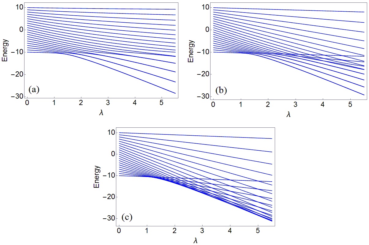
Figure 1: Spectrum of the LMG model as function of $\lambda$, for different values of $\gamma$. In panels (a), (b) and (c) we have $\gamma=0,\,0.5$ and $1$; respectively. In all cases $\omega_{0}=1$, and the number of particles is $N=20$.

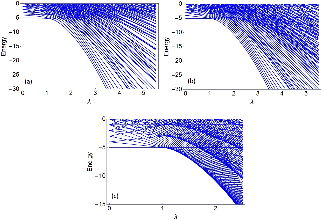
Figure 2: Spectrum of the Dicke model as function of $\lambda$, for different values of $\gamma$. In panels (a), (b) and (c) we have $\gamma=0,\,0.5$ and $1$; respectively. In all cases $\omega=\omega_{0}=1$, and the number of particles is $N=10$.

The quantum Hamiltonian for LMG model is defined by

$${\cal H}_{LMG}=-\omega_{0}J_{z}-\frac{\lambda}{N}\Bigl{(}J_{x}^{2}+\gamma\,J_{y}^{2}\Bigr{)}\,,$$ (1)

and the Hamiltonian for the full Dicke model reads

$${\cal H}_{D} =\omega\,a^{\dagger}a+\omega_{0}J_{z}$$

$$+\frac{\lambda(1+\gamma)}{2\sqrt{N}}\bigl{(}aJ_{+}+a^{\dagger}J_{-}\bigr{)}$$

$$+\frac{\lambda(1-\gamma)}{2\sqrt{N}}\bigl{(}aJ_{-}+a^{\dagger}J_{+}\bigr{)}\,.$$ (2)

For both cases, the angular momentum operators are $J_{\alpha}\equiv\frac{1}{2}\sum_{i=1}^{N}\sigma_{\alpha}^{(i)}$, where $\sigma_{\alpha}^{(i)}$ are the usual Pauli matrices associated to the $i$-two level system, with $\alpha=x,y,z$; $J_{\pm}\equiv J_{x}\pm iJ_{y}$; and the total angular momentum $(J_{x},J_{y},J_{z})$ represents collective transitions in the set of $N$ two-level atoms. In the Dicke model Hamiltonian, $a$ and $a^{\dagger}$ correspond to the creation and annihilation operators of the cavity bosonic mode. The energy gap between the two levels in each atom is $\omega_{0}$, the energy of the bosonic mode is $\omega$, and the adimensional parameter $0\leq\gamma\leq 1$ weights the $X$ and $Y$ direction of interaction in the LMG model and allows to weight the rotating term differently from the counterrotating term in the Dicke model.

The QPT is defined in the thermodynamic limit $N\rightarrow\infty$, since nonanalyticities appear in an order parameter at the transition. Both models exhibit a second order QPT, in the LMG model there is a transition from paramagnetic phase ($\lambda<\lambda_{C}=\omega_{0}$) to ferromagnetic phase ($\lambda>\lambda_{C}=\omega_{0}$) [31, 40], and in the Dicke model there is a transition from normal phase ($\lambda<\lambda_{C}=\sqrt{\omega\omega_{0}}$) to superradiant phase ($\lambda>\lambda_{C}=\sqrt{\omega\omega_{0}}$) [33, 34]. For the LMG and Dicke models we define the number excitation operator as $\hat{N}_{LMG}=J_{z}+N/2$ and $\hat{N}_{D}=a^{\dagger}a+J_{z}+N/2$ respectively. In both cases we define the parity operator as $\Pi=\mathrm{e}^{\mathrm{i}\pi\hat{N}}$ with the respective definition of the operator $\hat{N}$. Since for both models it is possible to verify that $[{\cal H},\Pi]=0$, they possess the discrete parity symmetry. In the special cases where $\gamma=1$ (isotropic LMG model and rotated wave approximation in Dicke model), they additionally possess the continuous symmetry $[\mathrm{e}^{\mathrm{i}\theta\hat{N}},{\cal H}]=0$ for any $\theta\in[0,2\pi)$, since $[{\cal H},\hat{N}]=0$. At the QPT, respective symmetries are broken [34, 40].

At finite values of $N$, the spectrum dependency on the coupling parameter $\lambda$ for the LMG and Dicke models are respectively given in Figs. 2 and 2. An important characteristic in both models when $\gamma=1$, is the level crossing for the lower energetic levels, in the ferromagnetic, and superradiant phases respectively. Such behavior is associated to the continuous symmetry of the models in the cases where $\gamma=1$ [22, 34].

By definition the QPT described above happens at zero temperature. In the Appendix A we show that at finite temperature the models exhibit the same phase transitions, it means, the same no-analytic behavior is found when the coupling parameter $\lambda$ changes, but no phase transition is observed when temperature changes, it means that no thermal phase transition is found. It is worth mentioning that this behavior happens when the atoms in the model are indistinguishable, for example this fact is studied in a restricted case of the Dicke model in Ref. [48]. On the other hand, when the particles are distinguishable, it is well known that there exists a thermal phase transition [33, 49, 50].

3 QUANTUM THERMODYNAMICS AND QUANTUM HEAT ENGINES

In this section we review briefly the notions of quantum thermodynamic in order to define our QHEs. We have that in the quantum domain the definitions of heat and work have to be revisited. In order to accomplish this we can use the standard approach to distinguish the different kinds of energy exchanges of the quantum system. Let us suppose that the system state is given by the density operator $\rho$ and that its dynamics is governed by the Hamiltonian ${\cal H}$. Hence, the system mean energy is given by $U=\text{Tr}\left({\rho{\cal H}}\right)$ and the energy exchange of the systems is

$$dU=\text{Tr}\left({d\rho\,{\cal H}}\right)+\text{Tr}\left({\rho\,d{\cal H}}\right)\,.$$ (3)

In Eq. (3), we identify the first term on the right hand side as the heat $\delta\langle Q\rangle$ absorbed by the system. This definition of heat is in agreement with the usual notion of heat as the energy variation associated with the change of the system internal state. Also, as we will see, this definition is compatible with the interpretation of heat as the energy variation related to an entropy increase. On the other hand, the second term in the right hand side of Eq. (3) is identified as the work performed over the system, which is equivalent to the negative of the work realized by the system $-\delta\langle W\rangle$. This definition relates work to the energy variation caused by changes in the external parameters that define the Hamiltonian of the system, as background fields or cavity size for example. It is worth mentioning that, in general work is process dependent and is not an observable, which probability distribution and characteristic function should be properly defined by a two-measurement protocol [51]. Therefore, we have that the mean values of absorbed heat and work realized by the quantum system in a thermodynamic transformation are

$$\langle Q\rangle =\int\text{Tr}\left({d\rho\,{\cal H}}\right),$$

$$\langle W\rangle =-\int\text{Tr}\left({\rho\,d{\cal H}}\right),$$ (4)

these quantities are path dependent and their values depend on the way that the density state, or the Hamiltonian, changes during the process. For our case, we assume that the system is always in thermal equilibrium with a thermal bath at temperature $\beta^{-1}$, and its density operator is a Gibbs state of the form

$$\rho(\beta,\lambda)=e^{-\beta{\cal H}(\lambda)}/{\cal Z}(\beta,\lambda),$$ (5)

where ${\cal Z}(\beta,\lambda)=\text{Tr}(e^{-\beta{\cal H}(\lambda)})$ is the partition function and ${\cal H}(\lambda)$ is the system Hamiltonian parametrized by a general external variable $\lambda$. In our study, we consider for ${\cal H}$ the LMG and Dicke Hamiltonian, where $\lambda$ is the coupling constant, which drives the QPT in each model. We also consider a quantum Stirling heat engine, defined by two isothermals (i. e. constant $\beta$) and two processes with fixed value of coupling constant $\lambda$, see Fig. 3. For these processes we are able to rewrite our formal expressions of mean quantum heat and mean quantum work. By using the notions of entropy and free energy

$$S =-\text{Tr}\left(\rho\ln\rho\right),$$

$$F =-\ln{\cal Z}/\beta,$$ (6)

one can show that if we are always on a Gibbs state Eq. (5) and the processes are such that probabilities are conserved, $\text{Tr}(d\rho)=0$, we have that

$$\langle Q\rangle =\int\frac{dS(\beta,\lambda)}{\beta},$$

$$\langle W\rangle =-\int\frac{\partial F(\beta,\lambda)}{\partial\lambda}d\lambda,$$ (7)

here we need to put into evidence that the entropy and free energy depend on both temperature $\beta^{-1}$ and the coupling constant $\lambda$. Hence, in general, the amount of heat absorbed and work realized by the system in a given process are path dependent. Nonetheless, the first law of thermodynamics is always obeyed, since for any infinitesimal process we have $dU=\delta\langle Q\rangle-\delta\langle W\rangle$. Therefore, in a finite process we have

$$\Delta U=\langle Q\rangle-\langle W\rangle.$$ (8)

For the Stirling QHE we have two kind of processes:
Isothermal transformation: In this process the temperature $\beta^{-1}$ of the system is kept constant by exchanging heat with a reservoir, and it realizes work over the environment. In this transformation the parameter $\lambda$ changes from some initial value $\lambda_{i}$ to a final one $\lambda_{f}$. Hence, from Eq. (7) we have that in an isothermal process, the heat and work respectively read

$$\langle Q\rangle_{isoth} =\Delta S/\beta=(S(\beta,\lambda_{f})-S(\beta,\lambda_{i}))/\beta,$$

$$\langle W\rangle_{isoth} =-\Delta F=-F(\beta,\lambda_{f})+F(\beta,\lambda_{i}).$$ (9)

$\lambda$-fixed transformation: In this process the external parameter $\lambda$, that defines the Hamiltonian, is kept constant while the temperature of the system $\beta^{-1}$ changes. Through the process, the system does not realizes any work, but it could exchange heat with the reservoir. Since in this case $\lambda$ remains constant and the temperature changes from some initial value $\beta^{-1}_{i}$ to a final one $\beta^{-1}_{f}$, we have from Eqs. (7) and (8) that in the $\lambda$-fixed process

$$\langle Q\rangle_{\lambda-fixed} =U(\beta_{f},\lambda)-U(\beta_{i},\lambda),$$

$$\langle W\rangle_{\lambda-fixed} =0.$$ (10)

As we just saw above, the thermodynamic processes depend on the internal energy $U$, entropy $S$ and free energy $F$, where they can be obtained from the partition function ${\cal Z}$. The computation of this partition function depends on the Hamiltonian and the Hilbert space of the system, therefore it is important to clearly define these two last physical aspects. In this work, the QHEs are defined by the LMG Hamiltonian ${\cal H}_{LMG}$ (see Eq. (1)) in one case, and the Dicke Hamiltonian ${\cal H}_{D}$ (see Eq. (2)) in the other. The angular momentum operators in both models are collective operators defined by $J_{\alpha}\equiv\frac{1}{2}\sum_{i=1}^{N}\sigma_{\alpha}^{(i)}$, with $\alpha=x,y,z$, and they are derived from a $N$ two-level atoms composition. The whole angular momentum Hilbert space is spanned by the set of states $\{|j,m\rangle\}$, where $j=\{0,1,...,\frac{N}{2}\}$ for $N$ even, or $j=\{\frac{1}{2},\frac{3}{2},...,\frac{N}{2}\}$ for $N$ odd, and $m=\{-j,-j+1,...,j-1,j\}$. The trace to be computed in the partition function of Eq. (5), depends on the Hilbert space of the models, where according to the nature of the experiment to realize the models, two possibilities are identified. The first one considers distinguishable two-level atoms, in this scenario the thermodynamics properties of the systems are well known [33, 49, 50]. The second possibility considers indistinguishable two-level atoms, in this situation the Hilbert space is restricted to the totally symmetric states under particle permutation operations. Indeed, instead of atoms, the physical realization for this case uses a set of bosonic particles in a collective two-level unique system. In the indistinguishable case, the Hilbert space is spanned by the set $\{|j,m\rangle\}$, where $j$ acquires the fixed maximum value $j=\frac{N}{2}$ whereas $m=\{-\frac{N}{2},-\frac{N}{2}+1,...,\frac{N}{2}-1,\frac{N}{2}\}$. For the thermodynamics in both models we have that in the distinguishable case there are both quantum and thermal phase transitions [33, 49, 50], while as we show in the Appendix A, for the indistinguishable case the thermal phase transition is absent. See also the Ref. [48] for the Dicke model in the ultrastrong-coupling limit case.

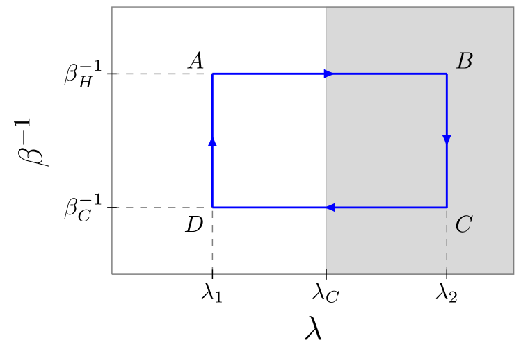
Figure 3: Stirling type cycle for the QHEs studied, in a temperature $\times$ coupling constant phase diagram. The vertical line over $\lambda_{C}$ represents the QPT for each model, and the white and gray shadow regions represent respectively the paramagnetic and ferromagnetic phases for the LMG model, and the normal and superradiant phases for the full Dicke model.

In the study of this paper we consider the indistinguishable case for both models. Moreover, the thermodynamic cycle of our QHEs is the Stirling cycle, it is shown in Fig. 3 and defined by the following processes:
Process $A\rightarrow B$: Isothermal process at fixed temperature $\beta_{H}^{-1}$. In this process the coupling constant $\lambda$ changes from $\lambda_{1}$ to $\lambda_{2}$, going through the critical value $\lambda_{C}$ when $\lambda_{2}>\lambda_{C}$. Here the absorbed heat of the system is given by

$$\langle Q\rangle_{AB}=(S_{B}-S_{A})/\beta_{H}>0\,.$$ (11)

Process $B\rightarrow C$: Process at fixed coupling constant $\lambda_{2}$. Here, the temperature of the system diminishes from $\beta_{H}^{-1}$ to $\beta_{C}^{-1}$. The system does not realize work but releases heat given by

$$\langle Q\rangle_{BC}=U_{C}-U_{B}<0\,.$$ (12)

Process $C\rightarrow D$: Isothermal process at fixed temperature $\beta_{C}^{-1}$. In this transformation the coupling constant $\lambda$ goes back from $\lambda_{2}$ to its initial value $\lambda_{1}$, going through the critical value $\lambda_{C}$ when $\lambda_{2}>\lambda_{C}$. In this process it releases heat given by

$$\langle Q\rangle_{CD}=(S_{D}-S_{C})/\beta_{C}<0\,.$$ (13)

Process $D\rightarrow A$: Process at fixed coupling constant $\lambda_{1}$. Here the temperature increases from $\beta_{C}^{-1}$ to $\beta_{H}^{-1}$. The system does not realize work but absorbs heat given by

$$\langle Q\rangle_{DA}=U_{A}-U_{D}>0\,.$$ (14)

For the whole cycle, the efficiency of the quantum Stirling heat engine is define by

$$\eta=\frac{\langle W\rangle}{\langle Q\rangle_{abs}}\,,$$ (15)

where $\langle W\rangle$ is the total work performed by the system and $\langle Q\rangle_{abs}=\langle Q\rangle_{AB}+\langle Q\rangle_{DA}$, is the amount of heat absorbed by the system. Since we have a cyclic process, and due to the first law of thermodynamics, we have $\langle W\rangle=\langle Q\rangle_{AB}+\langle Q\rangle_{BC}+\langle Q\rangle_{CD}+\langle Q\rangle_{DA}$.

4 RESULTS AND ANALYSIS

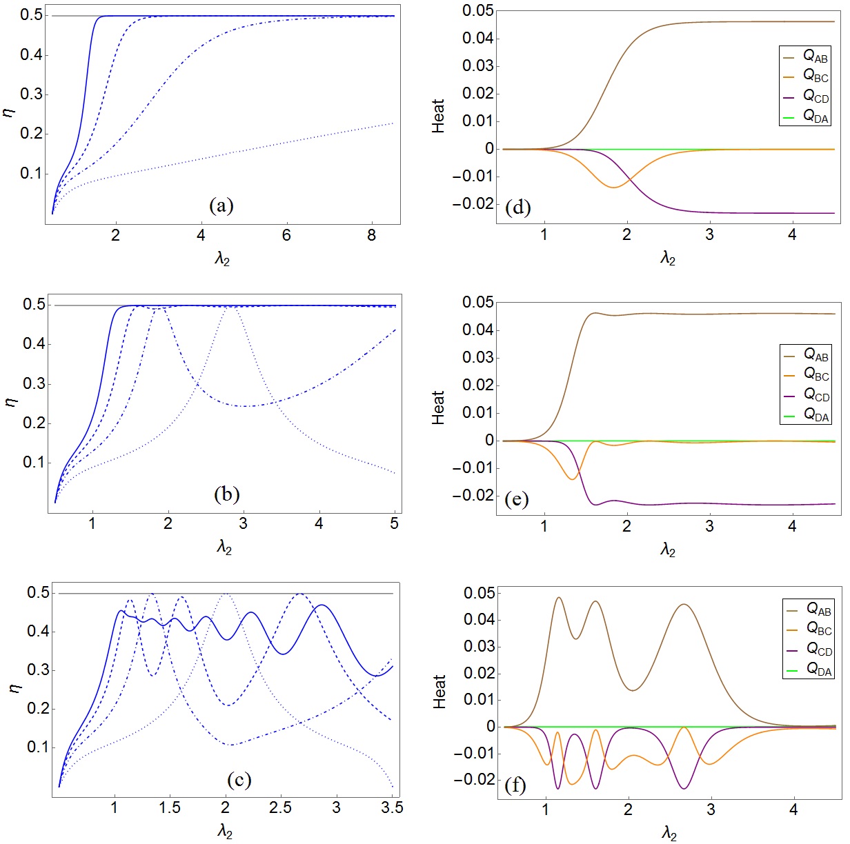
Figure 4: The QHE efficiency for the LMG model as function of $\lambda_{2}$, is shown in panels (a) for the completely anisotropic case $\gamma=0$, (b) for the anisotropic case with $\gamma=0.5$ and (c) for the isotropic case $\gamma=1$. For the three cases, the full, dashed, dot-dashed and dotted lines correspond to number of particles $N=20,\,8,\,4$ and $2$ respectively, and the gray upper line to the Carnot efficiency. The heat exchanged at each path of the cyclic process, see Fig. 3, as function of $\lambda_{2}$ are shown in panels (d) for the completely anisotropic case $\gamma=0$, (e) for the anisotropic case with $\gamma=0.5$ and (f) for the isotropic case $\gamma=1$; with $N=8$. For all the panels: $\omega_{0}=1$, $\beta_{C}^{-1}=1/30$, $\beta_{H}^{-1}=1/15$ and $\lambda_{1}=0.5$.

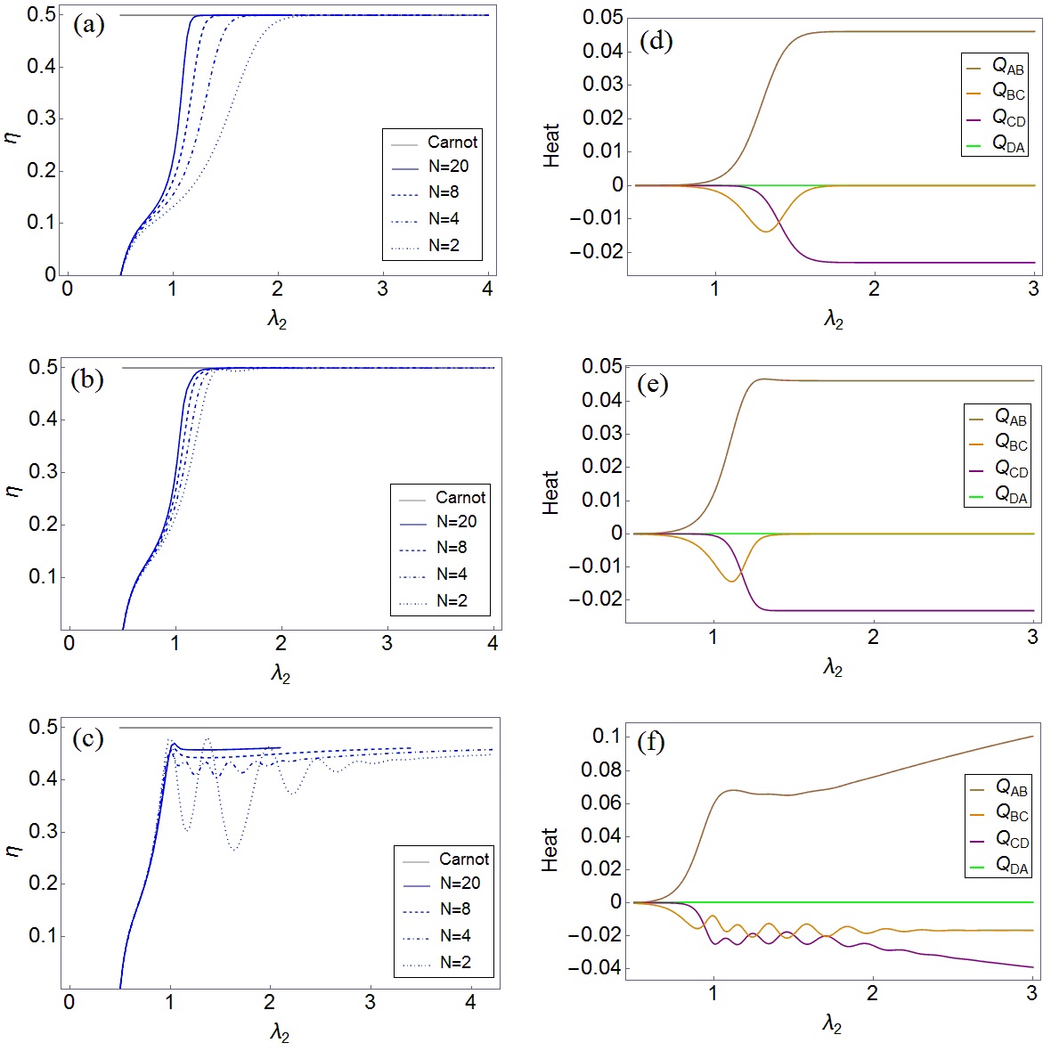
Figure 5: The QHE efficiency for the Dicke model as function of $\lambda_{2}$ is shown in panels (a) for the case $\gamma=0$ where rotating and counter-rotating terms are equally balanced, (b) for the unbalance case with $\gamma=0.5$ and (c) for the case where the rotating-wave approximation is considered and $\gamma=1$, for number of particles $N=20,\,8,\,4$ and $2$ as indicated. The gray upper line correspond to the Carnot efficiency. The heat exchanged at each path of the cyclic process, see Fig. 3, as function of $\lambda_{2}$ are shown in panels (d) for the case $\gamma=0$ where rotating and counter-rotating terms are equally balanced, (e) for the unbalance case with $\gamma=0.5$ and (f) for the case where the rotating-wave approximation is considered and $\gamma=1$; with $N=4$. For all the panels: $\omega=\omega_{0}=1$, $\beta_{C}^{-1}=1/30$, $\beta_{H}^{-1}=1/15$ and $\lambda_{1}=0.5$.

In this section we show numerical results for the efficiency of the QHEs defined in the last section. These systems are always at thermal equilibrium, then their states are defined by Gibbs states (see definition in Eq. (5)). In such context, the thermodynamic quantities are obtained from the partition function, which is computed by numerical diagonalization of respective Hamiltonian, given in Eqs. (1) and (2). For the full Dicke model case, this technique requires a cut-off in the infinite Hilbert space of the bosonic mode. The cut-off was set up demanding a good convergence of the numerical results.

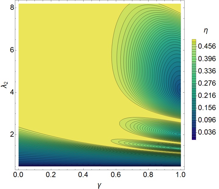
Figure 6: QHE efficiency for the LMG model as function of the anisotropy parameter $\gamma$ and coupling constant $\lambda_{2}$. The regions of high efficiency are find for small values of $\gamma$, (more anisotropic model), and high values of $\lambda_{2}$. In the regions of small $\gamma$, (more isotropic model), there appears regions of low efficiency. We used values $N=8$, $\omega_{0}=1$, $\beta_{C}^{-1}=15$, $\beta_{H}^{-1}=30$ and $\lambda_{1}=0.5$.

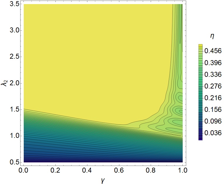
Figure 7: QHE efficiency for the Dicke model as function of the parameter $\gamma$ (that unbalances between rotating and counter-rotating terms) and coupling constant $\lambda_{2}$. The regions of high efficiency are find for small values of $\gamma$ and high values of $\lambda_{2}$. In the regions of small $\gamma$, (rotating-wave approximation implemented), there appears regions of low efficiency. We used values $N=4$, $\omega=\omega_{0}=1$, $\beta_{C}^{-1}=15$, $\beta_{H}^{-1}=30$ and $\lambda_{1}=0.5$.

The principal results for the anisotropic LMG and full Dicke models are shown in Figs. 4, 5, 7 and 7. In the calculations we set the atoms energy gaps $\omega_{0}=1$ and the bosonic energy excitations $\omega=1$, with such values the QPT occurs at $\lambda_{C}=1$ for both models. As defined in the last section, our QHEs follow a Stirling cycle (see Fig. 3), where the coupling constant of the initial state $A$ is fixed at $\lambda_{1}=0.5$, it means that the system starts in the paramagnetic phase for the LMG model, and in the normal phase for the Dicke model. In Figs. 4 and 5, several results are displayed when the coupling constant $\lambda_{2}$ (of states $B$ and $C$) varies from some minimum value $\lambda_{2}=0.5$ to some maximum, crossing in that interval the critical value $\lambda_{2}=\lambda_{C}=1$. The strict definition of phase transitions occurs for the limit $N\rightarrow\infty$ (see Appendix A), however we can see in the Figs. 4 and 5 that when the value of $N$ increases from $2$ to $20$, a convergent character of the efficiency is shown (a general analysis of finite-$N$ corrections for the studied models is found in [31, 34]). This behavior is justified because the efficiency is a quotient of energies, which despite not being analytical with $\lambda$, are continuous, and a discontinuity only appears in their second order derivative. So the cases of $N$ being finite but with an enough high value would provide a close approximation to the thermodynamic limit.

In general, Carnot engines are reversible heat engines, operating by two processes at constant temperature (using a cold and hot thermal baths for each one), and by two adiabatic processes (i. e. with no heat exchange). The QHEs studied in this paper follow a Stirling cycle type, defined by two isothermal processes $A\rightarrow B$ (hot temperature) and $C\rightarrow D$ (cold temperature), and by two processes where the coupling constant $\lambda$ is fixed, $B\rightarrow C$ and $D\rightarrow A$, see Fig. 3. From our results in panels (d), (e) and (f) of Figs. 4 and 5, for the LMG and Dicke models respectively, it is possible to note that Carnot bound is achieved when the exchanged heat in processes $BC$ and $DA$, i. e. $\langle Q\rangle_{BC}$ and $\langle Q\rangle_{DA}$, are zero (attention that panels (d), (e) and (f) correspond to the $N=8$ case). Therefore, for these particular cases, the QHE with Stirling cycle agrees with the Carnot engine definition, since heat exchange of the system only happens in the isothermal processes $AB$ and $CD$.

It is evident, from Figs. 4 and 5, that the efficiency has lower values when $\lambda_{2}$ satisfies $\lambda_{1}<\lambda_{2}<\lambda_{C}$, i. e. the whole cycle remains in the paramagnetic phase for the LMG model, or normal phase for the Dicke model. When we allow the systems undergo a QPT during the thermodynamic cycle, in such a way that points $B$ and $C$ of the cycle are now in the ferromagnetic phase for the LMG model and in the super-radiant phase for the Dicke model, i. e. $\lambda_{2}>\lambda_{C}$, we obtain a great enhancement of the cycle efficiency. Moreover in last cases, the cycle efficiency eventually achieves the Carnot bound. As was pointed out before, the efficiency is close or equal to the Carnot bound value when the heats $\langle Q\rangle_{BC}$ and $\langle Q\rangle_{DA}$ are close or equal to zero respectively. Moreover, it is known that degeneracies in the ground level energy appear when the systems undergo a QPT, and in the Appendix B we explore a relation between such degeneracies and high QHE efficiency. It is important to mention that such high efficiency values happen for low values of temperature, when the quantum behavior is dominant, in contrast with higher temperatures where the efficiency falls.

The degree of anisotropy in the LMG model and of unbalance between the rotating and counter-rotating terms in the full Dicke model, are controlled by the value of the parameter $\gamma$ in their respective Hamiltonians. The effect over the cycle efficiency due to the different values of $\gamma$ are shown in panels (a), (b) and (c) of Figs. 4 and 5 for the LMG and Dicke models, respectively. Setting the parameter $\gamma=0$, we have the most anisotropic coupling for the LMG model, and equal balance between rotating and counter-rotating terms for the full Dicke model. The results for this case of $\gamma=0$ is exhibited in panels (a), where we observe that the efficiency converges to the Carnot efficiency after $\lambda_{2}$ exceeds the critical value $\lambda_{C}$. We notice also that this convergence to maximum efficiency is more rapidly obtained when compared to cases of bigger values of $\gamma$ (those showed in panels (b) and (c)). In the cases where $\gamma<1$ but close to $1$ (the case $\gamma=1$ is exhibited in panel (c)), oscillatory values of efficiency appears as the coupling constant $\lambda_{2}$ changes, where such behavior is suppressed for lower values of $\gamma$. The Figs. 7 and 7, respectively correspond to the LMG model and the full Dicke model, where those figures show in contour plot graphics the behavior of the QHE efficiency for different values of the anisotropy parameter $\gamma$ and coupling constant $\lambda_{2}$. We notice that for small values $\gamma\approx 0$ (which corresponds to the more anisotropic case in the LMG model and the equally balance between rotating and counter-rotating terms in the Dicke model), the efficiency rapidly grows up to a maximum value, specially after $\lambda_{2}$ overpass $\lambda_{C}$ approximately. In the case of $\gamma\lesssim 1$ (near the completely isotropic case of the LMG model or when the rotating wave approximation is consider into the Dicke model), there appears regions of small efficiencies and the efficiency oscillates as we increase the values of $\lambda_{2}$ for fixed $\gamma$. We also found that as we increase the value of $N$, in that sense approaching to the thermodynamics limit, both the regions size of small efficiency and the amplitude of the efficiency oscillations (found when $\lambda_{2}$ changes but $\gamma$ is fixed) reduce.

The different dependence of efficiency with the parameter $\gamma$, indeed has its origin on the characteristics of the spectrum of the model (Fig. 2 and Fig. 2), and it is possible to see that as more level crossings there are, more accentuated are the oscillations of efficiency. In Appendix B we analyze in more detail the existence of a relation between level crossings energies (those close to the ground level) and high efficiency values. The same efficiency oscillations for the isotropic LMG model was reported in Ref. [23].

It is possible to extend the relation between the behavior of efficiency with the values of $\gamma$, to the symmetry of the models. In this case, as $\gamma$ gets closer to $1$, the continuous symmetry derived from $[{\cal H},\hat{N}]=0$ (see section 2) becomes dominant, in other words the respective interacting term with such symmetry ($J_{x}^{2}+J_{y}^{2}=J^{2}-J_{z}^{2}$ for the anisotropic LMG and the rotating term in the full Dicke model) gets dominant. Consequently when this continuous symmetry is broken at the phase transition there is an infinite degenerate ground state and therefore more crossings are expected to be present at the lower energetic levels for the finite $N$ model [22, 34]. On the other hand, when $\gamma$ gets different from $1$ (approaching to $0$) the continuous symmetric term becomes less relevant, and the Hamiltonian loses such symmetry, but keeps a discrete parity symmetric term. Consequently at the phase transition this symmetry is broken and a double degenerate ground state arise. In such situation, for the finite $N$ model the number of level crossings decrease at the lower energetic levels.

5 CONCLUSIONS

The efficiency of two QHEs were computed, each engine operates with different quantum critical systems, corresponding to the anisotropic LMG model in one case and the full Dicke model in the other, where the thermodynamic cycles are of Stirling type. For both models, we show numerical results for low temperatures, where optimization of the efficiency value (reaching the Carnot limit at some particular cases) was observed, it happens when during the cycle process the model undergoes a QPT.

A faster efficiency grow is obtained when the interaction term in the LMG model is more anisotropic than isotropic, and in the Dicke model when the interaction posses the rotating and counter-rotating terms equally balanced. It means, the rotating wave approximation (i. e. when the counter-rotating term is eliminated) is not appropriate to have a faster efficiency grow.

Is observed that Carnot and our Stirling cycles are equivalent at some particular values of the model parameters, where in such cases, there are heat transference only in the isothermal processes of the Stirling cycles. In that cases efficiency maximum values are attained and it is also noticed how the ground state degeneracies due to the QPT are associated to such maximum efficiencies. Such behavior is related to symmetries of the models, since symmetries rule the degeneracy of the ground state due to the QPT and also rule the existence of level crossings in the spectrum of the systems.

Is important to mention that the thermodynamics of the models studied here, correspond to indistinguishable particles in a two level system. For this situation, the Hilbert space of the set of $N$ particles is $N-$dimensional, and thermodynamic quantities are not extensive. A different behavior is observed for the distinguishable cases, which correspond to a set of $N$ two-level atoms. In such case the Hilbert space is $2^{N}-$ dimensional, and the thermodynamic quantities are extensive [52, 53]. In the last case thermal phase transitions are observed, nevertheless in the indistinguishable cases do not, where only appears QPT (see Appendix A and for the Dicke model in the ultrastrong-coupling regime [48]). An interesting extension of this work could be the analysis of QHEs when the substance corresponds to the same models studied in this work but in the distinguishable cases.

Appendix A Phase Transition at Finite Temperature

In this appendix we prove that at finite temperature the models exhibit a phase transition when changing the $\lambda$ coupling parameter, similar to the zero temperature case which defines the QPT. However, no phase transition appears when temperature is modified, such behavior is peculiar for the indistinguishable particles cases.

In order to prove this, we start using the Jordan-Schwinger map for the angular momentum Hilbert space and operators. According to such map, the relations for operators are the following,

$$J_{z} \rightarrow\frac{1}{2}(b_{1}^{\dagger}b_{1}-b_{2}^{\dagger}b_{2})\,,$$

$$J_{+} \rightarrow b_{1}^{\dagger}b_{2}\,,$$

$$J_{-} \rightarrow b_{2}^{\dagger}b_{1}\,,$$ (16)

where $b_{1}$ and $b_{2}$ are bosonic operators, it means, $[b_{i},b_{j}^{\dagger}]=\delta{ij}$ and $[b_{i},b_{j}]=[b_{i}^{\dagger},b_{j}^{\dagger}]=0$. And there is a one to one equivalence between the Hilbert space, given by the following map

$$|jm\rangle\rightarrow|n_{1}n_{2}\rangle\,,$$ (17)

where $n_{1}=j+m$ and $n_{2}=j-m$. Moreover $\{|jm\rangle\}$ is the standard basis for angular momentum Hilbert space and $\{|n_{1}n_{2}\rangle\}$ is a basis for the two bosons tensor product Hilbert space, where $b_{1}^{\dagger}b_{1}|n_{1}\rangle=n_{1}|n_{1}\rangle$ and $b_{2}^{\dagger}b_{2}|n_{2}\rangle=n_{2}|n_{2}\rangle$. Note that in general $j$ has an upper limit, and since $j=(n_{1}+n_{2})/2$, the sum $n_{1}+n_{2}$ should have an upper limit too. Additionally, for the models studied in this paper $j=N/2$, so the new equivalent Hilbert space for particles is restricted to the case where $n_{1}+n_{2}=N$, the total number of particles.

A more natural interpretation for the physical systems arises from the two boson Hilbert space, where the state $|n_{1}n_{2}\rangle$ is understood as $n_{1}$ indistinguishable particles being in one energetic level and $n_{2}$ indistinguishable particles in other, and the total particles number $N=n_{1}+n_{2}$ is fixed. Since $J_{z}\,|n_{1}n_{2}\rangle=\frac{1}{2}(n_{1}-n_{2})\,|n_{1}n_{2}\rangle$, the lower and higher energy of the levels depends on the sign preceding the $\omega_{0}\,J_{z}$ term in the Hamiltonian. For the LMG model we have $-\omega_{0}\,J_{z}\,|n_{1}n_{2}\rangle=\frac{1}{2}(-\omega_{0}n_{1}+\omega_{0}n_{2})\,|n_{1}n_{2}\rangle$, which means that $n_{1}$ indistinguishable particles are in a $-\omega_{0}/2$ energy level, and $n_{2}$ indistinguishable particles are in a $\omega_{0}/2$ energy level, therefore the second level is more energetic than the first one. For the full Dicke model we have $\omega_{0}\,J_{z}\,|n_{1}n_{2}\rangle=\frac{1}{2}(\omega_{0}n_{1}-\omega_{0}n_{2})\,|n_{1}n_{2}\rangle$, which means that $n_{2}$ indistinguishable particles are in a lower energy level $-\omega_{0}/2$, and $n_{1}$ indistinguishable particles are in a higher energy level $\omega_{0}/2$.

In order to study thermodynamic quantities, the partition function should be computed. Using the two boson Hilbert space representation of the models and the canonical ensemble, we have ${\cal Z}=\text{Tr}\left(e^{-\beta{\cal H}^{(B)}}\delta({\cal N}-N)\right)$, where ${\cal H}^{(B)}$ is the respective Hamiltonian for each model in terms of the bosonic operators, and ${\cal N}=b_{1}^{\dagger}b_{1}+b_{2}^{\dagger}b_{2}$. An useful mathematical relation for the delta function is adopted, $\delta({\cal N}-N)=\int dz\,e^{-\mathrm{i}z({\cal N}-N)}$, where since $[{\cal H},{\cal N}]=0$ the partition function results

$${\cal Z}=\int dz\,\text{Tr}\left(e^{-\beta{\cal H}^{(B)}-\mathrm{i}z({\cal N}-N)}\right)\,.$$ (18)

For computation of partition function given by Eq. (18) we resort to functional integration technique [50, 54]. Therefore, the partition functions are written as

$${\cal Z}_{LMG}=\int dz\int[d\eta(b_{1},b_{2})]\,e^{S_{LMG}[z,b_{1},b_{2}]}\,,$$ (19)

$${\cal Z}_{D}=\int dz\int[d\eta(a,b_{1},b_{2})]\,e^{S_{D}[z,a,b_{1},b_{2}]}\,,$$ (20)

where $[d\eta(b_{1},b_{2})]$ and $[d\eta(a,b_{1},b_{2})]$ are the respective functional measures and $S_{LMG}[z,b_{1},b_{2}]$ and $S_{D}[z,a,b_{1},b_{2}]$ are the Euclidean actions, given by

$$S_{LMG}[z,b_{1},b_{2}]= \int_{0}^{1}d\tau\,\Bigl{[}b_{1}(\tau)\partial_{\tau}b_{1}^{*}(\tau)+b_{2}(\tau)\partial_{\tau}b_{2}^{*}(\tau)$$

$$-\beta\,{\cal H}_{LMG}\bigl{(}b_{1}(\tau), b_{2}(\tau)\bigr{)}-\mathrm{i}\,z\Bigl{(}{\cal N}\bigl{(}b_{1}(\tau),b_{2}(\tau)\bigr{)}-N\Bigr{)}\Bigr{]}$$ (21)

$$S_{D}[z,a,b_{1},b_{2}]= \int_{0}^{1}d\tau\,\Bigl{[}a(\tau)\partial_{\tau}a^{*}(\tau)+b_{1}(\tau)\partial_{\tau}b_{1}^{*}(\tau)$$

$$+b_{2}(\tau) \partial_{\tau}b_{2}^{*}(\tau)-\beta\,{\cal H}_{D}\bigl{(}a(\tau),b_{1}(\tau),b_{2}(\tau)\bigr{)}$$

$$-\mathrm{i}\,z\Bigl{(}{\cal N}\bigl{(}b_{1}(\tau),b_{2}(\tau)\bigr{)}-N\Bigr{)}\Bigr{]}$$ (22)

where ${\cal H}_{LMG}\bigl{(}b_{1}(\tau),b_{2}(\tau)\bigr{)}$; ${\cal H}_{D}\bigl{(}a(\tau),b_{1}(\tau),b_{2}(\tau)\bigr{)}$ and ${\cal N}\bigl{(}b_{1}(\tau),b_{2}(\tau)\bigr{)}$ are defined by the original Hamiltonians and the number operator respectively, such that operators $a$, $b_{1}$ and $b_{2}$ were replaced by c-functions $a(\tau)$, $b_{1}(\tau)$ and $b_{2}(\tau)$ in the same order. Finally, applying the following scaling transformation $a(\tau)\rightarrow\sqrt{N}\,a(\tau)$, $b_{1}(\tau)\rightarrow\sqrt{N}\,b_{1}(\tau)$ and $b_{2}(\tau)\rightarrow\sqrt{N}\,b_{2}(\tau)$, we get

$${\cal Z}_{LMG}=\int dz\int[d\eta(b_{1},b_{2})]\,e^{N\,\Phi_{LMG}[z,b_{1},b_{2}]}\,,$$ (23)

$${\cal Z}_{D}=\int dz\int[d\eta(a,b_{1},b_{2})]\,e^{N\,\Phi_{D}[z,a,b_{1},b_{2}]}\,,$$ (24)

where the functionals $\Phi_{LMG}[z,b_{1},b_{2}]$ and $\Phi_{D}[z,a,b_{1},b_{2}]$ from equations above, reads

 

$$\Phi_{LMG}[z,b_{1},b_{2}]=\int_{0}^{1}d\tau\,\biggl{\{}b_{1}(\tau)\,\partial_{\tau}\,b_{1}^{*}(\tau)+b_{2}(\tau)\,\partial_{\tau}\,b_{2}^{*}(\tau)+\frac{\beta\omega_{0}}{2}\,\Bigl{(}b_{1}^{*}(\tau)b_{1}(\tau)-b_{2}^{*}(\tau)b_{2}(\tau)\Bigr{)}$$

$$+\frac{\beta\lambda}{4} \,\biggl{[}\Bigl{(}b_{1}^{*}(\tau)b_{2}(\tau)+b_{2}^{*}(\tau)b_{1}(\tau)\Bigr{)}^{2}-\gamma\Bigl{(}b_{1}^{*}(\tau)b_{2}(\tau)-b_{2}^{*}(\tau)b_{1}(\tau)\Bigr{)}^{2}\biggr{]}-\mathrm{i}\,z\Bigl{(}b_{1}^{*}(\tau)b_{1}(\tau)+b_{2}^{*}(\tau)b_{2}(\tau)-1\Bigr{)}\biggr{\}}\,,$$ (25)

$$\Phi_{D}[z,a,b_{1},b_{2}]=\int_{0}^{1}d\tau\,\biggl{\{}a(\tau)\partial_{\tau}a^{*}(\tau)+b_{1}(\tau)\,\partial_{\tau}\,b_{1}^{*}(\tau)+b_{2}(\tau)\,\partial_{\tau}\,b_{2}^{*}(\tau)-\beta\omega a^{*}(\tau)a(\tau)$$

$$-\frac{\beta\omega_{0}}{2}\,\Bigl{(}b_{1}^{*}(\tau)b_{1}(\tau)-b_{2}^{*}(\tau)b_{2}(\tau)\Bigr{)}-\frac{\beta\lambda(1+\gamma)}{2}\,\Bigl{(}a(\tau)b_{1}^{*}(\tau)b_{2}(\tau)+a^{*}(\tau)b_{2}^{*}(\tau)b_{1}(\tau)\Bigr{)}$$

$$-\frac{\beta\lambda(1-\gamma)}{2}\,\Bigl{(}a(\tau)b_{2}^{*}(\tau)b_{1}(\tau)+a^{*}(\tau)b_{1}^{*}(\tau)b_{2}(\tau)\Bigr{)}-\mathrm{i}\,z\Bigl{(}b_{1}^{*}(\tau)b_{1}(\tau)+b_{2}^{*}(\tau)b_{2}(\tau)-1\Bigr{)}\biggr{\}}\,.$$ (26)

 

Since the functional integrals in Eqs. (23) and (24) are not Gaussian, some approximation technique is required. Asymptotic expressions for the partition functions at thermodynamic limit ($N\rightarrow\infty$) are obtained from Eqs. (23) and (24), for this purpose the steepest descent method is used [50, 54]. According to such method, the biggest contributions come from the maximum value of $\Phi_{LMG}[z,b_{1},b_{2}]$ and $\Phi_{D}[z,a,b_{1},b_{2}]$, for each case. Such maximums values (and in general also minimum and saddle points) happen at $z$ value and $a(\tau)$, $b_{1}(\tau)$ and $b_{2}(\tau)$ functions satisfying the equations: $\frac{\partial\Phi_{LMG}}{\partial z}=0$; $\frac{\delta\Phi_{LMG}}{\delta b_{1}(\tau^{\prime})}=\frac{\delta\Phi_{LMG}}{\delta b_{1}^{*}(\tau^{\prime})}=0$; $\frac{\delta\Phi_{LMG}}{\delta b_{2}(\tau^{\prime})}=\frac{\delta\Phi_{LMG}}{\delta b_{2}^{*}(\tau^{\prime})}=0$ for the LMG model; and $\frac{\partial\Phi_{D}}{\partial z}=0$; $\frac{\delta\Phi_{D}}{\delta a(\tau^{\prime})}=\frac{\delta\Phi_{D}}{\delta a^{*}(\tau^{\prime})}=0$; $\frac{\delta\Phi_{D}}{\delta b_{1}(\tau^{\prime})}=\frac{\delta\Phi_{D}}{\delta b_{1}^{*}(\tau^{\prime})}=0$; $\frac{\delta\Phi_{D}}{\delta b_{2}(\tau^{\prime})}=\frac{\delta\Phi_{D}}{\delta b_{2}^{*}(\tau^{\prime})}=0$ for the full Dicke model. A simplifying fact is that solutions of last maximization equations are constant functions, i.e. $a(\tau)=a_{0}=r_{0}\,e^{\mathrm{i}\,\theta_{0}}$, $b_{1}(\tau)=b_{10}=r_{1}\,e^{\mathrm{i}\,\theta_{1}}$, $b_{2}(\tau)=b_{20}=r_{2}\,e^{\mathrm{i}\,\theta_{2}}$ and respective complex conjugates. After solving the last equations we obtain maximum and saddle point solutions, where the maximum solutions correspond to:

The LMG model:
For $\lambda<\omega_{0}$: $z=-\frac{\mathrm{i}\beta\omega_{0}}{2}$; $b_{10}=1$ and $b_{20}=0$.
For $\lambda\geq\omega_{0}$: $z=-\frac{\mathrm{i}\beta\lambda}{2}$; $r_{1}=\sqrt{\frac{\lambda+\omega_{0}}{2\lambda}}$ and $r_{2}=\sqrt{\frac{\lambda-\omega_{0}}{2\lambda}}$; where for the anisotropic case $\gamma\neq 1$ the difference of phases $\Delta\theta=\theta_{2}-\theta_{1}$ has two possibilities $\Delta\theta=\{0,\pi\}$; and for the isotropic case $\gamma=1$ the difference of phases is any value $0\leq\Delta\theta<2\pi$.

Computing the energy according to $U_{LMG}=-\partial_{\beta}\ln{\cal Z}_{LMG}$, we have

$$\frac{U_{LMG}}{N}=\left\{\begin{array}[]{cc}-\frac{\omega_{0}}{2}&\mbox{se: }\lambda<\lambda_{c}\,,\\ -\frac{1}{4}\left(\lambda+\frac{\omega_{0}^{2}}{\lambda}\right)&\mbox{se: }\lambda\geq\lambda_{c}\,,\end{array}\right.$$ (29)

where $\lambda_{c}=\omega_{0}$ is the critical coupling and entropy $S_{LMG}=\beta U_{LMG}+\ln{\cal Z}_{LMG}=0$.

The full Dicke model:
For $\lambda<\sqrt{\omega\omega_{0}}$: $z=-\frac{\mathrm{i}\beta\omega_{0}}{2}$; $a_{0}=b_{10}=0$ and $b_{20}=1$.
For $\lambda\geq\sqrt{\omega\omega_{0}}$: $z=-\frac{\mathrm{i}\beta\lambda^{2}}{2\omega}$; $r_{0}=\sqrt{\frac{(\lambda^{2}-\omega\omega_{0})(\lambda^{2}+\omega\omega_{0})}{4\omega^{2}\lambda^{2}}}$; $r_{1}=\sqrt{\frac{\lambda^{2}-\omega\omega_{0}}{2\lambda^{2}}}$ and $r_{2}=\sqrt{\frac{\lambda^{2}+\omega\omega_{0}}{2\lambda^{2}}}$; where for the anisotropic case $\gamma\neq 1$ the phase $\theta_{0}$ and difference of phases $\Delta\theta$ have two possibilities $(\theta_{0},\Delta\theta)=\{(0,\pi);(\pi,0)\}$ while for the isotropic case $\gamma=1$, the phase $\theta_{0}$ and the difference of phases $\Delta\theta$ are any value since $\theta_{0}+\Delta\theta=\pi$.

Computing the energy according to $U_{D}=-\partial_{\beta}\ln{\cal Z}_{D}$, we have

$$\frac{U_{D}}{N}=\left\{\begin{array}[]{cc}-\frac{\omega_{0}}{2}&\mbox{se: }\lambda<\lambda_{c}\,,\\ -\frac{\lambda^{2}}{4\omega}\left(1+\frac{\omega^{2}\omega_{0}^{2}}{\lambda^{4}}\right)&\mbox{se: }\lambda\geq\lambda_{c}\,,\end{array}\right.$$ (32)

where $\lambda_{c}=\sqrt{\omega\omega_{0}}$ is the critical coupling and entropy $S_{D}=\beta U_{D}+\ln{\cal Z}_{D}=0$.

From Eqs. (29) and (32) it is not difficult to prove that $\frac{d^{2}U}{d\lambda^{2}}$ is discontinuous at respective $\lambda_{c}$. In Fig. 8 we show the behavior of the specific energy and of its second order derivative in $\lambda$ for the LMG model. Due to the similarity between Eqs. (29) and (32), for the full Dicke model the last behavior described above is quite similar to the LMG model. Such results prove that the phase transition is of second order for both models, and no critical temperature $\beta_{c}^{-1}$ was found, which means that our models do not exhibit thermal phase transition for the indistinguishable particles cases.

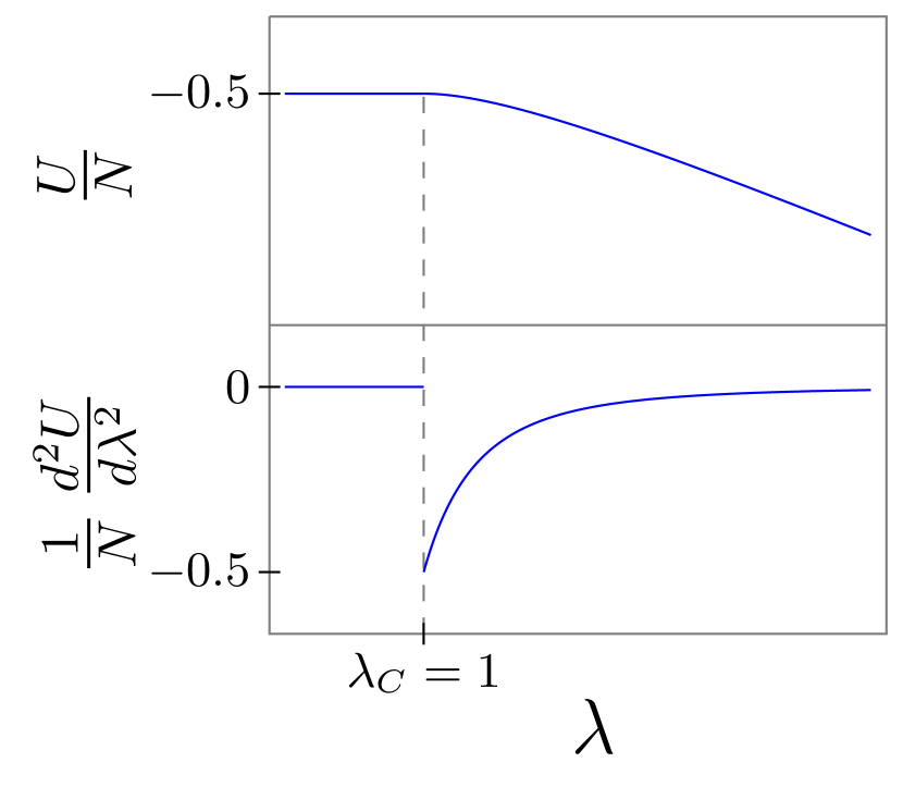
Figure 8: Specific energy of the LMG model and its second order derivative in $\lambda$. Here we can evidence the second order phase transition of the model.

Appendix B Ground state double degeneracy and efficiency increase in QHE

In this appendix we closely examine the relationship between the efficiency increase of the QHEs and the appearance of a double degeneracy in the ground energy level during the process. It is known that for the models studied in this work, such behavior happens at the QPT. The appearance of a double degeneracy is observed also in Figs. 2 and 2. In order to do the examination aforementioned, we analyze a simpler system (toy system). This system possess 4 energy levels dependent on some external parameter $\lambda$, in such a way that by modifying its value we are able to control the existence of the level crossings. Let us set the four energy levels given by $E_{1}(\lambda)=3\lambda$, $E_{2}(\lambda)=1+\lambda$, $E_{3}(\lambda)=5-\lambda$ and $E_{4}(\lambda)=12-3\lambda$; plotted in Fig.(9).

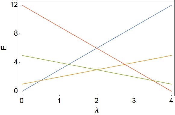
Figure 9: Crossing energy levels of a toy system. Each curve and respective energies function are: blue for $E_{1}(\lambda)=3\lambda$, yellow for $E_{2}(\lambda)=1+\lambda$, green for $E_{3}(\lambda)=5-\lambda$ and red for $E_{4}(\lambda)=12-3\lambda$.

There we can see that for values of $\lambda$ lower that $0.5$, the ground state corresponds to the first energy level $E_{1}(\lambda)$, but as $\lambda$ is increased the ground state changes $|E_{1}\rangle\rightarrow|E_{2}\rangle\rightarrow|E_{3}\rangle\rightarrow|E_{4}\rangle$. We also identify three values of $\lambda$ where the lower energetic level crossings happen, at $\lambda=\{0.5,2,3.5\}\,.$ Similar as our study of the LMG and full Dicke model, we calculate the partition function for this toy system assuming thermal equilibrium with a reservoir at temperature $\beta^{-1}$, it means, the partition function is: ${\cal Z}(\beta,\lambda)=\sum_{i=1}^{i=4}e^{-\beta\,E_{i}(\lambda)}$. Moreover, the QHE cycle is of the Stirling type, as defined in section 3, see Fig. 3.

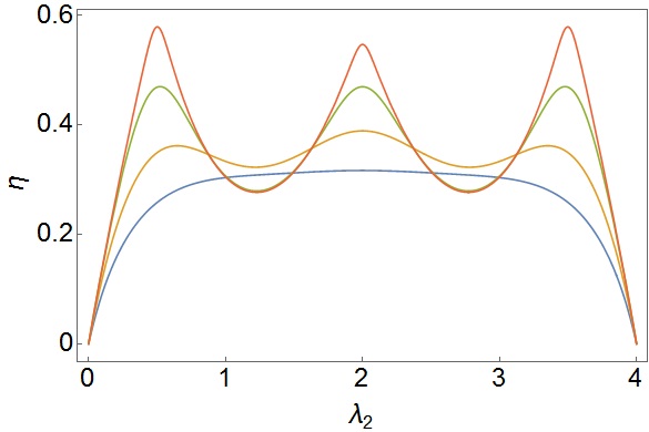
Figure 10: Graphs of efficiency function for the toy system at thermal equilibrium in an Stirling cycle (see Fig. 3). In whole the curves: $\lambda_{1}=0$, hot reservoir temperature $\beta_{H}^{-1}=2$ and $\lambda_{2}$ varies from $0$ to $4$. Temperature values of the cold reservoir are $\beta_{C}^{-1}=1$ for the blue curve, $\beta_{C}^{-1}=0.5$ for the yellow curve, $\beta_{C}^{-1}=0.2$ for the green curve and $\beta_{C}^{-1}=0.05$ for the red curve.

Results for the QHE efficiency are shown in Fig. 10, where some cycle parameter values are $\lambda_{1}=0$ and $\lambda_{2}$ varies from $0$ to $4$. So when $\lambda_{2}$ goes through a level crossings (at values $\lambda_{2}=\{0.5,2,3.5\}$) an increase of efficiency happens. It is noticed also that such increase is more accentuated at low temperatures.

According to the efficiency definition (see Eq. (15)) it is calculated by $\eta=1-\frac{|\langle Q\rangle_{BC}|+|\langle Q\rangle_{CD}|}{\langle Q\rangle_{AB}+\langle Q\rangle_{DA}}$. The heats exchanged at each part of the cycle are shown in Fig. 11, and it is evident from it that higher efficiency values are attained principally because the absolute value $|\langle Q\rangle_{BC}|$ is lower at the level crossing points.

In Stirling cycle (see Fig. 3), $|\langle Q\rangle_{BC}|$ represents one part of the heat released by the QHE, therefore, if it is lower then the work value increases, so increasing the efficiency. From Eq. (12) we have $\langle Q\rangle_{BC}=U_{C}-U_{B}$, where its absolute value is lower if the value of $U_{C}$ is closer to $U_{B}$. The difference between the energies $U_{C}$ and $U_{B}$ is caused by their different temperatures $\beta_{C}^{-1}$ and $\beta_{H}^{-1}$ respectively, then $U_{C}$ and $U_{B}$ will have close values each other when the principal energy level contributions to the mean energy $U$, i. e. the ground and first excited levels, are closer between them; such situation happens at $\lambda_{2}$ values around the degeneracy ground level points. In summary, the modification of the energy level population at the process $BC$ of the cycle costs less heat when ground level crossings occur.

Consequently, for low temperatures the ground state degeneracy becomes relevant to the increase of efficiency of our QHEs. Such degeneracies are characteristic of QPT models, present respectively in the ferromagnetic phase of the LMG model, and in the superradiant phase of the full Dicke model.

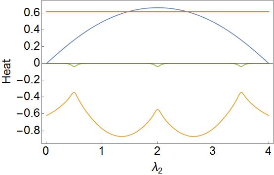
Figure 11: Heats involved in the QHE process for the toy system, according to the Stirling cycle (see Fig. 3). Was set the values: cold and hot reservoirs temperatures respectively are $\beta_{C}^{-1}=0.05$ and $\beta_{H}^{-1}=2$, $\lambda_{1}=0$ and $\lambda_{2}$ varies from $0$ to $4$. The blue line is for $\langle Q\rangle_{AB}$, yellow line for $\langle Q\rangle_{BC}$, green line for $\langle Q\rangle_{CD}$ and red line for $\langle Q\rangle_{DA}$.

References

- [1] André Xuereb. James Millen. Perspective on quantum thermodynamics. New. J. Phys., 18:011002, Jan 2016.
- [2] Zeeya Merali. The new thermodynamics: how physics is bending the rules. Nature, 551:20, Nov 2017.
- [3] Robert Alicki and Ronnie Kosloff. Introduction to quantum thermodynamics: History and prospects. arXiv, 1801.08314v2, May 2018.
- [4] Michael A. Nielsen and Isaac L. Chuang. Quantum Computation and Quantum Information: 10th Anniversary Edition. Cambridge University Press, New York, NY, USA, 10th edition, 2011.
- [5] Robert Alicki. The quantum open system as a model of the heat engine. J. Phys. A: Math. Gen., 12:L103, Jan 1979.
- [6] Tien D. Kieu. The second law, maxwell’s demon, and work derivable from quantum heat engines. Phys. Rev. Lett., 93:140403–1, Sep 2004.
- [7] Wolfgang Niedenzu, Victor Mukherjee, Arnab Ghosh, Abraham G Kofman, and Gershon Kurizki. Quantum engine efficiency bound beyond the second law of thermodynamics. Nature communications, 9(1):165, 2018.
- [8] J. Roßnagel, O. Abah, F. Schmidt-Kaler, K. Singer, and E. Lutz. Nanoscale heat engine beyond the carnot limit. Phys. Rev. Lett., 112:030602, Jan 2014.
- [9] Wolfgang Niedenzu, David Gelbwaser-Klimovsky, Abraham G Kofman, and Gershon Kurizki. On the operation of machines powered by quantum non-thermal baths. New Journal of Physics, 18(8):083012, aug 2016.
- [10] Gonzalo Manzano, Fernando Galve, Roberta Zambrini, and Juan M. R. Parrondo. Entropy production and thermodynamic power of the squeezed thermal reservoir. Phys. Rev. E, 93:052120, May 2016.
- [11] Jan Klaers, Stefan Faelt, Atac Imamoglu, and Emre Togan. Squeezed thermal reservoirs as a resource for a nanomechanical engine beyond the carnot limit. Phys. Rev. X, 7:031044, Sep 2017.
- [12] Bo Xiao and Renfu Li. Finite time thermodynamic analysis of quantum otto heat engine with squeezed thermal bath. Physics Letters A, 382(42):3051 – 3057, 2018.
- [13] Shanhe Su, Yanchao Zhang, Guozhen Su, and Jincan Chen. The carnot efficiency enabled by complete degeneracies. Physics Letters A, 382(32):2108 – 2112, 2018.
- [14] Bartłomiej Gardas and Sebastian Deffner. Thermodynamic universality of quantum carnot engines. Phys. Rev. E, 92:042126, Oct 2015.
- [15] Johannes Roßnagel, Samuel T. Dawkins, Karl N. Tolazzi, Obinna Abah, Eric Lutz, Ferdinand Schmidt-Kaler, and Kilian Singer. A single-atom heat engine. Science, 352(6283):325–329, 2016.
- [16] James Klatzow, Jonas N. Becker, Patrick M. Ledingham, Christian Weinzetl, Krzysztof T. Kaczmarek, Dylan J. Saunders, Joshua Nunn, Ian A. Walmsley, Raam Uzdin, and Eilon Poem. Experimental demonstration of quantum effects in the operation of microscopic heat engines. Phys. Rev. Lett., 122:110601, Mar 2019.
- [17] Hadrien Vroylandt, Massimiliano Esposito, and Gatien Verley. Collective effects enhancing power and efficiency. EPL (Europhysics Letters), 120(3):30009, nov 2017.
- [18] J Jaramillo, M Beau, and A del Campo. Quantum supremacy of many-particle thermal machines. New Journal of Physics, 18(7):075019, jul 2016.
- [19] Ali Ü. C. Hardal, Mauro Paternostro, and Özgür E. Müstecaplıoğlu. Phase-space interference in extensive and nonextensive quantum heat engines. Phys. Rev. E, 97:042127, Apr 2018.
- [20] Thao P. Le, Jesper Levinsen, Kavan Modi, Meera M. Parish, and Felix A. Pollock. Spin-chain model of a many-body quantum battery. Phys. Rev. A, 97:022106, Feb 2018.
- [21] Wolfgang Niedenzu and Gershon Kurizki. Cooperative many-body enhancement of quantum thermal machine power. New Journal of Physics, 20(11):113038, nov 2018.
- [22] Subir Sachdev. Quantum Phase Transitions. Cambridge University Press, 2 edition, 2011.
- [23] Yu-Han Ma, Shan-He Su, and Chang-Pu Sun. Quantum thermodynamic cycle with quantum phase transition. Phys. Rev. E, 96:022143, Aug 2017.
- [24] Michele Campisi and Rosario Fazio. The power of a critical heat engine. Nature communications, 7:11895, 2016.
- [25] Michal Kloc, Pavel Cejnar, and Gernot Schaller. Collective performance of a finite-time quantum otto cycle. Phys. Rev. E, 100:042126, Oct 2019.
- [26] Mojde Fadaie, Elif Yunt, and Özgür E. Müstecaplıoğlu. Topological phase transition in quantum-heat-engine cycles. Phys. Rev. E, 98:052124, Nov 2018.
- [27] H. J. Lipkin, N. Meshkov, and A. J. Glick. Validity of many-body approximation methods for a solvable model. Nucl. Phys., 62(2):188–198, 1965.
- [28] H. J. Lipkin, N. Meshkov, and A. J. Glick. Validity of many-body approximation methods for a solvable model. Nucl. Phys., 62(2):199–210, 1965.
- [29] H. J. Lipkin, N. Meshkov, and A. J. Glick. Validity of many-body approximation methods for a solvable model. Nucl. Phys., 62(2):211–224, 1965.
- [30] R. H. Dicke. Coherence in spontaneous radiation processes. Phys. Rev., 93:99–110, Jan 1954.
- [31] Sébastien Dusuel and Julien Vidal. Continuous unitary transformations and finite-size scaling exponents in the lipkin-meshkov-glick model. Phys. Rev. B, 71:224420, Jun 2005.
- [32] F. Leyvraz and W. D. Heiss. Large- scaling behavior of the lipkin-meshkov-glick model. Phys. Rev. Lett., 95:050402, Jul 2005.
- [33] Klaus Hepp and Elliott H Lieb. On the superradiant phase transition for molecules in a quantized radiation field: the dicke maser model. Annals of Physics, 76(2):360 – 404, 1973.
- [34] Clive Emary and Tobias Brandes. Chaos and the quantum phase transition in the dicke model. Phys. Rev. E, 67:066203, Jun 2003.
- [35] Julien Vidal, Guillaume Palacios, and Rémy Mosseri. Entanglement in a second-order quantum phase transition. Phys. Rev. A, 69:022107, Feb 2004.
- [36] N. Lambert, C. Emary, and T. Brandes. Entanglement and entropy in a spin-boson quantum phase transition. Phys. Rev. A, 71:053804, May 2005.
- [37] D. C. Meredith, S. E. Koonin, and M. R. Zirnbauer. Quantum chaos in a schematic shell model. Phys. Rev. A, 37:3499–3513, May 1988.
- [38] Tobias Graß, Bruno Juliá-Díaz, Marek Kuś, and Maciej Lewenstein. Quantum chaos in su(3) models with trapped ions. Phys. Rev. Lett., 111:090404, Aug 2013.
- [39] W D Heiss, F G Scholtz, and H B Geyer. The largeNbehaviour of the lipkin model and exceptional points. Journal of Physics A: Mathematical and General, 38(9):1843–1851, feb 2005.
- [40] Pedro Ribeiro, Julien Vidal, and Rémy Mosseri. Exact spectrum of the lipkin-meshkov-glick model in the thermodynamic limit and finite-size corrections. Phys. Rev. E, 78:021106, Aug 2008.
- [41] P. Pérez-Fernández, P. Cejnar, J. M. Arias, J. Dukelsky, J. E. García-Ramos, and A. Relaño. Quantum quench influenced by an excited-state phase transition. Phys. Rev. A, 83:033802, Mar 2011.
- [42] Tobias Brandes. Excited-state quantum phase transitions in dicke superradiance models. Phys. Rev. E, 88:032133, Sep 2013.
- [43] Kristian Baumann, Christine Guerlin, Ferdinand Brennecke, and Tilman Esslinger. Dicke quantum phase transition with a superfluid gas in an optical cavity. Nature, 464:1301–6, 04 2010.
- [44] Markus P. Baden, Kyle J. Arnold, Arne L. Grimsmo, Scott Parkins, and Murray D. Barrett. Realization of the dicke model using cavity-assisted raman transitions. Phys. Rev. Lett., 113:020408, Jul 2014.
- [45] Selçuk Çakmak, Ferdi Altintas, and Özgür E. Müstecaplıoğlu. Lipkin-meshkov-glick model in a quantum otto cycle. The European Physical Journal Plus, 131(6):197, Jun 2016.
- [46] Lorenzo Fusco, Mauro Paternostro, and Gabriele De Chiara. Work extraction and energy storage in the dicke model. Phys. Rev. E, 94:052122, Nov 2016.
- [47] Dario Ferraro, Michele Campisi, Gian Marcello Andolina, Vittorio Pellegrini, and Marco Polini. High-power collective charging of a solid-state quantum battery. Phys. Rev. Lett., 120:117702, Mar 2018.
- [48] M. Aparicio Alcalde, M. Bucher, C. Emary, and T. Brandes. Thermal phase transitions for dicke-type models in the ultrastrong-coupling limit. Phys. Rev. E, 86:012101, Jul 2012.
- [49] F. T. Hioe. Phase transitions in some generalized dicke models of superradiance. Phys. Rev. A, 8:1440–1445, Sep 1973.
- [50] M. Aparicio Alcalde and B.M. Pimentel. Path integral approach to the full dicke model. Physica A: Statistical Mechanics and its Applications, 390(20):3385 – 3396, 2011.
- [51] Peter Talkner, Eric Lutz, and Peter Hänggi. Fluctuation theorems: Work is not an observable. Phys. Rev. E, 75:050102, May 2007.
- [52] Pavel Cejnar and Pavel Stránský. Heat capacity for systems with excited-state quantum phase transitions. Physics Letters A, 381(11):984 – 990, 2017.
- [53] P. Pérez-Fernández and A. Relaño. From thermal to excited-state quantum phase transition: The dicke model. Phys. Rev. E, 96:012121, Jul 2017.
- [54] V.N. Popov and V.S. Yarunin. Collective Effects in Quantum Statistics of Radiation and Matter. Mathematical Physics Studies. Springer Netherlands, 1988.