Adaptive Online Learning for Gradient-Based Optimizers

Abstract

As application demands for online convex optimization accelerate, the need for designing new methods that simultaneously cover a large class of convex functions and impose the lowest possible regret is highly rising. Known online optimization methods usually perform well only in specific settings, and their performance depends highly on the geometry of the decision space and cost functions. However, in practice, lack of such geometric information leads to confusion in using the appropriate algorithm. To address this issue, some adaptive methods have been proposed that focus on adaptively learning parameters such as step size, Lipschitz constant, and strong convexity coefficient, or on specific parametric families such as quadratic regularizers. In this work, we generalize these methods and propose a framework that competes with the best algorithm in a family of expert algorithms. Our framework includes many of the well-known adaptive methods including MetaGrad, MetaGrad+C, and Ader. We also introduce a second algorithm that computationally outperforms our first algorithm with at most a constant factor increase in regret. Finally, as a representative application of our proposed algorithm, we study the problem of learning the best regularizer from a family of regularizers for Online Mirror Descent. Empirically, we support our theoretical findings in the problem of learning the best regularizer on the simplex and $l_{2}$-ball in a multiclass learning problem.

1 Introduction

Online Convex Optimization (OCO) plays a pivotal role in modeling various real-world learning problems such as prediction with expert advice, online spam filtering, matrix completion, recommender systems on data streams and large-scale data Hazan et al. (2016). The formal setting an OCO is described as follows.

OCO Setting

In OCO problem Cesa-Bianchi and Lugosi (2006); Hazan et al. (2016); Shalev-Shwartz et al. (2012), at each round $t$, we play $x_{t}\in\mathcal{D}$ where $\mathcal{D}\subseteq\mathbb{R}^{d}$ is a convex set. The adversarial environment incurs a cost $f_{t}(x_{t})$ where $f_{t}(x)$ is a convex cost function on $\mathcal{D}$ at iteration $t$. The main goal of OCO is to minimize the cumulative loss of our decisions. Since losses can be chosen adversarially by the environment, we use the notion of Regret as the performance metric, which is defined as

$$\mathcal{R}_{T}\triangleq\sum\limits_{t=1}^{T}f_{t}(x_{t})-\min\limits_{x\in\mathcal{D}}\sum\limits_{t=1}^{T}f_{t}(x).$$ (1.1)

In fact, regret measures the difference between the cumulative loss of our decisions and the best static decision in hindsight. In the literature, various iterative algorithms for OCO problem try to minimize regret and provide sublinear upper bound on it. All these algorithms are variations of Online Gradient Descent (OGD); meaning that these algorithms share a common feature in their update rule Hazan et al. (2016); Shalev-Shwartz et al. (2012); Duchi et al. (2011). Furthermore, their updating process is performed just based on previous decision points and their gradients. We call this family of OCO as Gradient-Based algorithms. In this paper, our attention is mainly drawn to this family of algorithms. Some of these algorithms such as Online Newton Steps Hazan et al. (2007) and AdaGrad Duchi et al. (2011); McMahan and Streeter (2010) have considered a specific class of cost functions like strongly-convex, exp-concave, and smooth functions. Then, by manipulating the step size and using second-order methods, they have been able to reach a better regret bound than $\mathcal{O}(\sqrt{T})$ Hazan et al. (2007). If we have no other restriction than convexity on cost functions, then the Regularization based algorithms such as Follow The Regularized Leader (FTRL) (Hazan et al., 2016, page 72) and Online Mirror Descent (Hazan et al., 2016, page 76) step into the field. In these algorithms, the geometry of the domain space $\mathcal{D}$ has been taken into account and in spite of the fact that their regret’s upper bound remains $\mathcal{O}(\sqrt{T})$, the constant factor of their regret bound can be improved by choosing a suitable regularizer.

Each Gradient-Based algorithm that performs on Lipschitz functions has the regret upper-bound $\mathcal{O}(\sqrt{T})$ and based on (Hazan et al., 2016, page 45) this bound is tight ($i.e.$ for each algorithm there is a sequence of cost functions whose regret is $\Omega(\sqrt{T})$). However, the constant factor in these algorithms is different.

In summary, there exists a group of iterative algorithms each of them has a number of tuning parameters. Consequently, in OCO setting it is very important to choose the right algorithm with the best set of parameters such that it results to the lowest regret bound w.r.t. the geometry of space and choice of cost functions. However, due to lack of our knowledge about the problem setup, it is not always possible to choose the right algorithm or tuning parameters. Our aim is to introduce a master algorithm that can compete with the best of such iterative algorithms in terms of regret bound.

1.1 Related Works

It is known that OGD achieves $\mathcal{O}(\sqrt{T})$ regret bound (Hazan et al., 2016, page 43) . In addition, if cost functions are strongly convex, then the regret bound $\mathcal{O}(\log{T})$ can be achieved Shalev-Shwartz et al. (2012). It is shown that Online Newton Step for exponentially concave cost functions has $\mathcal{O}(d\log{T})$ regret bound Hazan et al. (2007).

Considering adaptive frameworks, numerous approaches have been proposed in the literature to learn the parameters of OGD algorithm like step-size van Erven and Koolen (2016) and diameter of $\mathcal{D}$ Cutkosky and Boahen (2017). For tuning regularizer, one can mention AdaGrad algorithm that learns from a family of Quadratic Matrix regularizers Duchi et al. (2011). AdaGrad is a special case of the work presented in McMahan and Streeter (2010) that uses a family of increasing regularizers. MetaGrad algorithm that was proposed later than AdaGrad in van Erven and Koolen (2016) has the ability to learn the step-size for all Gradient-Based algorithms. However, it has high time complexity and needs many oracle accesses per iteration.

2 Preliminaries

In this section, we will introduce the notation that will be used throughout the paper and review some of the preliminary materials required to introduce our method.

2.1 Notation

We keep the following notation throughout the rest of paper. We use $V_{1:n}$ to denote a sequence of vectors $(V_{1},\ldots,V_{n})$. Let $x_{t}$ and $f_{t}$ be our decision and cost function respectively, then $\nabla_{t}$ denotes $\nabla f_{t}(x_{t})$. For cost function $f_{t}(x)$, surrogate cost function is denoted by $\widehat{f}_{t}(x)=\left\langle\nabla_{t},x\right\rangle$. Denote the upper bound on surrogate cost functions by $F=\sup\limits_{t\in\mathbb{N},x\in\mathcal{D}}|\left\langle\nabla f_{t}(x),x\right\rangle|$. Projection of vector $y$ on domain $\mathcal{D}$ w.r.t. some function or norm $R$ is denoted by $\operatorname{\Pi}_{\mathcal{D}}^{R}(y)$. Moreover, we denote by $\mathbb{B}_{p}$ the unit ball in $\mathbb{R}^{d}$ for $\ell_{p}$ norm, i.e., $\mathbb{B}_{p}^{d}=\{x\in\mathbb{R}^{d}\mid\|x\|_{p}\leq 1\}$. Also, we denote $\Delta(n)$ to be the $n$-simplex, i.e., $\Delta(n)=\{x\in\mathbb{R}_{+}^{n}\mid\mathbf{1}^{\top}x=1\}$. Finally, each OCO algorithm has its own regret bound on a family of cost functions. To refer to the regret bound of an arbitrary algorithm $\mathcal{A}$ after $T$ iterations, we use the notation $\mathcal{B}_{T}^{\mathcal{A}}$.

Definition 2.1.

As mentioned in Section 1, Gradient-Based algorithms are algorithms whose update rule is performed just based on previous decision points and their gradients. So for an arbitrary Gradient-Based algorithm A, we have an iterative update rule $x_{t}=\Psi_{A}(x_{t-1},\nabla_{1:t-1})$ and a non-iterative or closed form update rule denoted by $x_{t}=\Upsilon_{A}(x_{0},\nabla_{1:t-1})$.

In general, it can be difficult to derive the closed form for an algorithm. However, for some algorithms like OGD, Online Mirror Descent (OMD), AdaGrad, etc., $\Upsilon$ can be efficiently computed and eventually, attain the same complexity as $\Psi$. In Proposition 2.8, we show how to efficiently compute the update rules of OMD and AdaGrad.

2.2 Problem Statement

In this work, we focus on learning the best algorithm among a family of OCO algorithms. We also define the problem of learning the best regularizer as a special yet important case of learning the best OCO algorithm. Both problems are explicitly defined in the following.

Best OCO Algorithm: Let $\mathcal{D}\in\mathbb{R}^{d}$ be a compact convex set that presents the search domain of an OCO Algorithm. Our focus is on Gradient-Based algorithms, so we have a family $\mathcal{M}\triangleq\{\mathsf{OCO}_{1},\ldots,\mathsf{OCO}_{k}\}$ of algorithms where the update rule of the $i$-th algorithm is given by $x_{t+1}=\Psi_{i}(x_{t},\nabla_{1:t})$. Our goal is to propose an algorithm that perform as good as the best algorithm in $\mathcal{M}$.

Best Regularizer: When the family of algorithms only contains OMD algorithms, each member of $\mathcal{M}$ is completely characterized by its Regularizer. We consider $\mathsf{OMD}_{\varphi}$ as an OMD algorithm with Regularizer $\varphi(x)$. Now, let $\Phi\triangleq\{\varphi_{1}(x),\ldots,\varphi_{k}(x)\}$ be the set of regularizers in which the $i$-th element is $\eta_{i}$ strongly convex w.r.t. a norm $\|\cdot\|_{i}$. So we have a set of OMD algorithms with regularizers $\Phi$ denoted by $\mathcal{M}=\{\mathsf{OMD}_{\varphi_{1}},\ldots,\mathsf{OMD}_{\varphi_{k}}\}$. Moreover, we have an OCO problem similar to the “best OCO algorithm” defined above, that at each iteration decides based on the performance of all OMD algorithms in $\mathcal{M}$ (more precisely, best of them).

2.3 Expert Advice

Suppose we have access to $k$ experts $a_{1},\ldots,a_{k}$. At each round $t$, we want to decide based on the decisions of experts and then incur some loss $\ell_{t}(a_{t})\in[0,1]$ from the environment as feedback. This problem can be cast into the Online Learning in which to evaluate the goodness of an algorithm, the notion of Regret is used. Here, we use $\mathcal{R}_{T}(a^{*})=\sum_{t=1}^{T}\ell_{t}(a_{t})-\sum_{t=1}^{T}\ell_{t}(a^{*})$ to denote the regret of expert $a^{*}$. All algorithms for expert advice problem, follow the iterative framework described below Cesa-Bianchi and Lugosi (2006); Freund and Schapire (1997); Vovk (1990); Bubeck et al. (2012); Vovk (1998); Littlestone and Warmuth (1994) .

Expert Advice Framework

Let $p_{t}$ be the probability of choosing experts in each iteration. Suppose that based on prior knowledge we have a distribution $p_{1}$ over experts. If we have no idea about the experts, $p_{1}$ can be chosen to have a uniform distribution. At iteration $t$, we choose expert $a_{t}\propto p_{t}$ and play the decision made by $a_{t}$. Then the loss vector $\ell_{t}$ can be observed. We will update the probabilites $p_{t+1}$ based on losses we have observed until now.

In the expert advice framework, we can have two different settings based on the availability of feedbacks, stated as follows. (1) Full feedback setting where all experts losses $\ell_{t}$ are observed. (2) Limited feedback setting, or the so called Bandit Bubeck et al. (2012) version, where only $\ell_{t}(a_{t})$ is observed.

In what follows, the regret bounds of two well known algorithms namely Hedge Freund and Schapire (1997) and Squint are explained. We will elaborate on exponential-weight algorithm for exploration and exploitation (EXP3) Auer et al. (2002a) and gradient based prediction algorithm (GBPA) Abernethy et al. (2015) in the bandit setting.

Theorem 2.2 (Freund and Schapire (1997)).

Hedge algorithm, defined by choosing $p_{t}(a)\propto\exp\left(-\eta\sum\limits_{\tau=1}^{t-1}\ell_{\tau}(a)\right)$ in the expert advice framework, ensures   $\mathbb{E}\left(\mathcal{R}_{T}(a^{*})\right)\leq\frac{\log(K)}{\eta}+\eta T\leq 2\sqrt{\log(K)T}.$

Theorem 2.3 (Koolen and Van Erven (2015)).

Let $r_{t}(i)=\left\langle p_{t},\ell_{t}\right\rangle-\ell_{t}(i)$ and $V_{T}(a)=\sum\limits_{t=1}^{T}r_{t}(a)^{2}$. Then the Squint algorithm, defined by $p_{t}(a)\propto p_{1}(a)\exp\left(-\eta\sum\limits_{\tau=1}^{t-1}r_{\tau}(a)+\eta^{2}\sum\limits_{\tau=1}^{t-1}r_{\tau}(a)^{2}\right)$ in the expert advice framework, ensures $\mathbb{E}(\mathcal{R}_{T}(a^{*}))\leq\frac{ln(1/p_{1}(a^{*})}{\eta}+\eta V_{T}(a^{*})\leq 2\sqrt{V_{T}(a^{*})ln(1/p_{1}(a^{*}))}$.

Theorem 2.4 (Abernethy et al. (2015)).

GBPA algorithm, uses estimated loss $\widehat{\ell}_{t}=\frac{\ell_{t}(a_{t})}{p_{t}(a_{t})}\mathbb{e}_{a_{t}}$ and update rule $p_{t}(a)\propto\nabla(\eta S_{\alpha})^{*}\big{(}-\eta\sum\limits_{r=1}^{t-1}\widehat{\ell}_{r}(a)\big{)}$ in the expert advice framework, where $S_{\alpha}$ is Tsallis entropy with parameter $\alpha$, ensures $\mathbb{E}(\mathcal{R}_{T}(a^{*}))\leq\eta\frac{K^{1-\alpha}-1}{1-\alpha}+\frac{K^{\alpha}T}{2\eta\alpha}\leq 4\sqrt{KT}$ where $\alpha$ chooses as $1/2$.

Corollary 2.5.

In Theorem 2.4, if $\alpha\rightarrow 1$ leads to $p_{t}(a)\propto\exp\big{(}-\frac{1}{\eta}\sum\limits_{r=1}^{t-1}\widehat{\ell}_{r}(a)\big{)}$. So EXP3 algorithm is recovered and ensures  $\mathbb{E}(\mathcal{R}_{T}(a^{*}))\leq\eta\log(K)+\frac{TK}{2\eta}\leq\sqrt{2K\log(K)T}$.

Remark 2.6.

If we know that $\forall i,t:\ell_{t}(i)<L$, then in all expert advice theorems, the regret bounds will be multiplied by a factor $L$.

2.4 Online Mirror Descent

Definition 2.7 (Online Mirror Descent).

Update rule $\Psi$ for lazy and agile versions of OMD with regularizer $\varphi$ are defined as

$$Agile: \hskip 14.22636ptx_{t+1}=\Psi(x_{t},\nabla_{1:t})=\operatorname{\Pi}_{\mathcal{D}}^{\varphi}(\nabla\varphi^{*}(x_{t}-\eta\nabla_{t})),$$ (2.1)

$$Lazy: \hskip 14.22636pty_{t+1}=\Psi(y_{t},\nabla_{1:t})=\nabla\varphi^{*}(y_{t}-\eta\nabla_{t}),x_{t+1}=\operatorname{\Pi}_{\mathcal{D}}^{\varphi}(y_{t+1}).$$

Proposition 2.8.

Computing the closed form of $x_{t}$ for agile version of OMD is very complicated but for lazy update rule, we have $y_{t+1}=\Upsilon(y_{t},\nabla_{1:t})=\operatorname{\Pi}_{\mathcal{D}}^{\varphi}\big{(}\nabla\varphi^{*}(x_{0}-\eta\sum_{i=1}^{t}\nabla_{i})\big{)}$. Thus, the computation of $\Upsilon$ is light weighted because we need only to keep $S_{t}=\sum_{i=1}^{t}\nabla_{i}$ in each iteration.

3 Proposed Methods

Our proposed methods for the problem stated in Section 2.2, are inspired by expert advice problem. First, we propose an algorithm that uses expert advice in full feedback setting and then for the sake of time complexity, present another algorithm that has almost the same regret as the former algorithm

3.1 Assumptions

Here, we review three assumptions in this work. (1) All cost functions are Lipschitz w.r.t some norm $\|x\|_{.}$ on $\mathcal{D}$, i.e., there exists $L_{.}>0$ such that $\forall x,y\in\mathcal{D}:|f(x)-f(y)|\leq L_{.}\|x-y\|_{.}$. (2) Domain $\mathcal{D}$ contains the origin (if not can be translated) and is bounded w.r.t. some norm $\|x\|_{.}$, i.e., there exists $D_{.}>0$ such that $\forall x,y\in\mathcal{D}:\|x-y\|_{.}<D$. (3) Suppose $\mathcal{A}$ is an arbitrary OCO algorithm that performs on $L$-Lipschitz cost functions, w.r.t. an arbitrary norm $\|\cdot\|_{.}$, and domains with diameter $D$, w.r.t. the same norm. Then, there exists a tight upper bound $\mathcal{B}_{T}^{\mathcal{A}}$ on the regret $\mathcal{R}_{T}^{\mathcal{A}}$ that $\mathcal{A}$ achieve this bound. Hence $\mathcal{B}_{T}^{\mathcal{A}}$ depends on the parameters $L$, $D$, and $T$.

3.2 Master OCO Framework

By the problem setting described in Section 2.2, we have $K$ experts and each of these experts is a Gradient-Based algorithm. In order to learn the Best OCO Algorithm, we will take advantage of expert advice algorithms.

Framework Overview: In our proposed framework, called Master OCO Framework , we consider an expert advice algorithm $\mathcal{A}$ and a family of online optimizers. We want to exploit the expert advice algorithm to track the best optimizer in hindsight. In each round, $\mathcal{A}$ selects an optimizer $a_{t}$ to see its prediction $x_{t}^{a_{t}}$. Environment reveals cost function $f_{t}(x)$. Then we pass the surrogate cost function $\widehat{f}_{t}(x)=\left\langle\nabla_{t},x\right\rangle$ to all optimizers instead of the original cost function. Hence, to be consistent with the expert advice scenario assumptions, we consider normalized surrogate cost function for losses. So we’ll have $\ell_{t}(i)=\widehat{f}_{t}(x_{t}^{i})/(2F)+1/2$, where $F$ is an upper bound for surrogate functions. Now, based on full or partial feedback assumption of $\mathcal{A}$, we pass $\{\ell_{t}(i)\}_{i\in[K]}$ or $\ell_{t}(a_{t})$ to $\mathcal{A}$, respectively. Finally, $\mathcal{A}$ updates probability distribution $p_{t}$ over experts based on the observed losses.

Remark 3.1.

The main reason why we use surrogate function in place of the original cost function is as follows. Considering the $i$-th expert, using surrogate function leads to generating a sequence of decisions $\{x_{t}^{i}\}_{t\in[T]}$. This is just similar to the situation where we merely use the $i$-th expert algorithm on an OCO problem whose cost functions at iteration $t$ are $\hat{f_{t}}(x)$. We will prove this claim in Appendix B.

In the following the formal description of our framework is provided.

Framework 1 Master OCO Framework

1:  Input: Expert advice algorithm $\mathcal{A}$, set of online optimizers $\mathcal{M}=\{\mathsf{OCO}_{i}\}_{i\in[K]}$

2:  for t = 1, …, T do

3:     $\mathcal{A}$ decides what optimizer $a_{t}\in[K]$ should be selected

4:     Ask selected optimizer to get prediction $x_{t}^{a_{t}}$

5:     Play $x_{t}=x_{t}^{a_{t}}$ and the environment incurs a cost function $f_{t}(x)$

6:     Pass the surrogate cost function $\widehat{f}_{t}(x)=\left\langle\nabla_{t},x\right\rangle$ to all optimizers

7:     Select $S=[K]$ or $S=\{a_{t}\}$ based on partial or fully feedback property of $\mathcal{A}$

8:     Set losses for the observed predictions: $\forall i\in S:\ell_{t}(i)=\frac{\widehat{f}_{t}(x_{t}^{i})}{2F}+\frac{1}{2}$

9:     Pass $\{\ell_{t}^{i}\}_{i\in S}$ to $\mathcal{A}$. Now $\mathcal{A}$ can update the probabilities over the experts

10:  end for

Proposition 3.2.

Let $\mathcal{M}=\{\mathsf{OCO}_{i}\}_{i\in[K]}$ be Gradient-Based optimizers and $\mathcal{A}$ be an expert advice algorithm. Then for all $\mathsf{OCO}_{i}\in\mathcal{M}$, our proposed framework ensures

$$\mathcal{R}_{T}\leq 2F\cdot\mathcal{R}_{T}^{\mathcal{A}}+\mathcal{R}_{T}^{\mathsf{OCO}_{i}},$$ (3.1)

where $F$ is a tight upper bound for all surrogate cost functions, $\mathcal{R}_{T}^{\mathsf{OCO}_{i}}$ is the regret of running $i$-th optimizer on surrogate functions and $\mathcal{R}_{T}^{\mathcal{A}}$ is the general regret of expert advice algorithm $\mathcal{A}$.

Remark 3.3.

In general, there is no need to normalize the cost functions. In fact we can pass surrogate cost functions as losses $\ell_{t}(i)=\widehat{f}_{t}(x_{t}^{i})$ and gain the same regret bound as mentioned above. So without knowing $F$, we can still apply the above framework.

Corollary 3.4.

In expert advice algorithm $\mathcal{A}$, suppose $p_{t}$ is the probability distribution over optimizers at iteration $t$. If we have access to all optimizers’ predictions $\{x_{t}^{i}\}_{i\in[K]}$, we can play in determinist way, namely, $x_{t}=\mathbb{E}(x_{t}^{a_{t}})=\sum_{i=1}^{T}p_{t}(i)x_{t}^{i}$ and thus, obtain a regret bound of $\mathbb{E}(\mathcal{R}_{T})$ in (3.1).

Corollary 3.5.

If we choose the expert advice algorithm $\mathcal{A}$ such that $\mathcal{R}_{T}^{\mathcal{A}}$ is comparable to the best of $\{\mathcal{R}_{T}^{\mathsf{OCO}_{i}}\}$, then using $\mathcal{A}$ in our framework results in achieving a regret bound that is comparable with the best optimizers in $\mathcal{M}$.

In order to compare these regret bounds, we need to introduce an important lemma. Thus, Lemma 3.6 will help us compare $\mathcal{R}_{T}^{\mathcal{A}}$ and $\mathcal{R}_{T}^{\mathsf{OCO}_{i}}$ appeared in proposition 3.2.

Lemma 3.6 (Main Lemma).

Let $\mathcal{A}$ be an arbitrary OCO algorithm that performs on $L$-Lipschitz cost functions, w.r.t. some norm $\|\cdot\|_{.}$, and domains with diameter $D$, w.r.t. the same norm. Then, the regret bound for this algorithm, i.e., $\mathcal{B}_{T}^{\mathcal{A}}$, is lower bounded by $\Omega(LD\sqrt{T})$.

It should be emphasized that in Framework 1, the availability of feedback is in our control by choosing $S$ as $\{\ell_{t}(i)\}_{i\in[K]}$ or $\ell_{t}(a_{t})$. In fact choice of $S$ is based on the full or partial feedback property of $\mathcal{A}$. Note that although having limited feedback might result in an increase of regret, but it also causes a reduction in computational complexity of the proposed algorithm. In Section 3.3 and Section 3.4, we will elaborate more on this trade-off. In the following, we exploit two choices of expert advice algorithms, namely, Squint and GBPA, which result in proposing Master Gradient Descent (MGD) and Fast Master Gradient Descent (FMGD), respectively.

3.3 Master Gradient Descent

Consider Framework 1 with Squint as the expert advice algorithm. We call this algorithm Master Gradient Descent (MGD) that is described in Algorithm 2.

Algorithm 2 Master Gradient Descent (MGD)

  Input: Learning rate $\eta>0$, family of optimizers $\mathcal{M}=\{\mathsf{OCO}_{i}\}_{i\in[K]}$ with update rules $\{\Psi_{i}\}_{i\in[K]}$

  Initialization: Let $R_{0},V_{0}\in\mathbb{R}^{K},x_{0}\in\mathbb{R}^{d}$ be all-zero vectors, $p_{1}\in\Delta(K)$ be uniform distribution

  for $t=1,\ldots,T$ do

     for $a=1,\ldots,k$ do

        Run the $a$-th optimizer algorithm and attain $x_{t}^{a}=\Psi_{a}(x_{t-1}^{a},\nabla_{1:t-1})$

     end for

     Play $x_{t}=\sum_{a=1}^{k}p_{t}(a)x_{t}^{a}$ and observe cost function $f_{t}(x)$

     Pass surrogate cost function $\widehat{f}_{t}(x)=\left\langle\nabla_{t},x\right\rangle$ to all optimizers

     Set loss for the $a$-th expert as: $\ell_{t}(a)=\frac{\widehat{f}_{t}(x_{t}^{a})}{2F}+\frac{1}{2}$

     Let $\forall i:r_{t}(i)=\left\langle p_{t},\ell_{t}\right\rangle-\ell_{t}(i)$ then update $R_{t}=R_{t-1}+r_{t}$ , $\forall i:V_{t}(i)=V_{t-1}(i)+r_{t}(i)^{2}$

     Compute $p_{t+1}\in\Delta(K)$ such that $p_{t+1}(i)\propto p_{1}(i)\exp(-\eta R_{t}(i))+\eta^{2}V_{t}(i))$

  end for

Based on Proposition 3.2 and Lemma 3.6, we can provide a regret bound for the MGD algorithm, as stated in Theorem 3.7. The detailed proof is provided in Appendix B.

Theorem 3.7.

Consider MGD algorithm with a set of Gradient-Based optimizers $\mathcal{M}$. Suppose $\mathsf{OCO}_{i}$ is an arbitrary optimizer in $\mathcal{M}$ under assumptions stated in Section 3.1, MGD ensures

$$\mathcal{R}_{T}\leq 4F\sqrt{V_{T}(i)\ln K}+\mathcal{R}_{T}^{\mathsf{OCO}_{i}}=\mathcal{O}\left(\sqrt{\ln K}\mathcal{B}_{T}^{\mathsf{OCO}_{i}}\right),$$

where $F$ is the tight upper bound for all cost functions, $\mathcal{B}_{T}^{\mathsf{OCO}_{i}}$ is also the tight regret upper bound for $\mathsf{OCO}_{i}$ algorithm and $V_{T}(i)=\sum_{t=1}^{T}(\left\langle p_{t},\ell_{t}\right\rangle-\ell_{t}(i))^{2}$.

Remark 3.8.

If we use Hedge as expert advice algorithm in Framework 1 nstead of Squint, it achieve the same regret bound as Theorem 3.7.

Remark 3.9.

The value of $V_{T}(i)$ can be much smaller than $T$, so the regret of MGD can be bounded by the best regret among all optimizers.

Corollary 3.10.

Theorem 3.7 shows that the Master Gradient Descent framework gives a comparable regret bound with the best algorithms of $\mathcal{M}$ in hindsight.

3.4 Fast Master Gradient Descent

Although MGD only needs one oracle access to cost functions $\{f_{t}\}_{t\in[T]}$, it needs to apply update rules of all $K$ optimizers simultaneously in each iteration. So its computational cost is higher than a Gradient-Based algorithm. However, if the closed form of the update rule $\Upsilon$ can be computed efficiently same as computing iterative update rule $\Psi$, then we can provide an algorithm that can effectively reduce MGD time complexity up to factor $\frac{1}{K}$.

We will show that the proposed algorithm, named Fast Master Gradient Descent , achieves almost same regret bound as MGD. This algorithm is obtained from Framework 1 in partial feedback setting that uses GBPA as its expert advice algorithm. ␣‌GBPA uses Tsallis entropy $S_{\alpha}(x)$ and its Fenchel conjugate which is introduced in Appendix A.1. According to Corollary 2.5, if $\alpha\rightarrow 1$ then EXP3 is also covered. The details of FMGD is described in Algorithm 3. We provide a regret bound for FMGD, as stated in Theorem 3.11. The detailed proof is provided in Appendix B.

Algorithm 3 Fast Master Gradient Descent (FMGD)

  Input: Learning rate $\eta>0$, family of optimizers $\mathcal{M}=\{\mathsf{OCO}_{i}\}_{i\in[K]}$ with closed form update rules $\{\Upsilon_{i}\}_{i\in[K]}$

  Initialization: Let $\widehat{L}_{0}\in\mathbb{R}^{K},x_{0}\in\mathbb{R}^{d}$ be all-zero vectors and $p_{1}\in\Delta(K)$ be the uniform distribution over the family of optimizers $\mathcal{M}$

  for $t=1,\ldots,T$ do

     Choose $a_{t}\sim p_{t}$ as an action

     Run the $a_{t}$-th expert algorithm and attain $x_{t}=\Upsilon_{a_{t}}(x_{0},\nabla_{1:t-1})$

     Observe cost function $f_{t}$

     Set loss for the $a_{t}$-th expert as: $\ell_{t}(a_{t})=\frac{\widehat{f}_{t}(x_{t})}{2F}+\frac{1}{2}=\frac{\left\langle\nabla_{t},x_{t}\right\rangle}{2F}+\frac{1}{2}$

     Update $\widehat{L}_{t}=\widehat{L}_{t-1}+\widehat{\ell}_{t}$ where $\forall a\in[K]:\widehat{\ell}_{t}(a)=\frac{\ell_{t}(a)}{p_{t}(a)}\textbf{1}\{a=a_{t}\}$

     Compute $p_{t+1}\in\Delta(K)$ such that $p_{t+1}\propto\nabla S_{\alpha}^{*}\left(-\frac{\widehat{L}_{t}}{\eta}\right)$

  end for

Theorem 3.11.

Consider FMGD algorithm with optimizer set $\mathcal{M}$ that consists of Gradient-Based optimizers. Then for all optimizers $\mathsf{OCO}_{i}\in\mathcal{M}$, under assumptions stated in Section 3.1, FMGD ensures

$$\alpha=1/2\ (GBPA):\mathbb{E}(\mathcal{R}_{T})\leq 8F\sqrt{TK}+\mathcal{B}_{T}^{\mathsf{OCO}_{i}}=\mathcal{O}\left(\sqrt{K}\mathcal{B}_{T}^{\mathsf{OCO}_{i}}\right),$$

$$\alpha\rightarrow 1\ (EXP3):\mathbb{E}(\mathcal{R}_{T})\leq 2F\sqrt{2TK\ln K}+\mathcal{B}_{T}^{\mathsf{OCO}_{i}}=\mathcal{O}\left(\sqrt{K\ln K}\mathcal{B}_{T}^{\mathsf{OCO}_{i}}\right),$$

where $F$ is a tight upper bound for all surrogate cost functions and $\mathcal{B}_{T}^{\mathsf{OCO}_{i}}$ is the tight upper bound regret for $\mathsf{OCO}_{i}$ algorithm.

Corollary 3.12.

In regret bound term, FMGD attains same regret bound as MGD (differs by at most $\sqrt{K/\ln K}$ multiplicative factor). In computational terms, if for each members of $\mathcal{M}$, the closed form update rule $\Upsilon$ can be computed with the same complexity as $\Psi$, then in the worst case FMGD achieves the same complexity as the worst complexity of algorithms in $\mathcal{M}$. Hence, its computational complexity is improved by a multiplicative factor of $\frac{1}{K}$.

3.5 Learning The Best Regularizer

Consider the problem described in Section 2.2, where we have $K$ lazy-OMD algorithms (described in Definition 2.7) that are determined by $K$ different regularizer functions. Now, in order to compete with the best regularizer, we can take advantage of MGD algorithm with its optimizers set $\mathcal{M}$ consisting of lazy-OMD algorithms. According to Proposition 2.8, closed form of update rules for lazy-OMD algorithms, can be computed efficiently by keeping track of $S_{t}=\sum_{i=1}^{t}\nabla_{i}$ in each iteration. Consequently, based on what is stated in Corollary 3.12, using FMGD leads to learning the best regularizer with low computational cost.

Now in Theorem 3.13 we express our results on learning the best regularizer among a family of regularizers.

Theorem 3.13.

Let $\Phi$ be a set of $K$ regularizers in which the $i$-th member $\varphi_{i}\colon\mathcal{D}\to\mathbb{R}$ is $\rho_{i}$-strongly convex w.r.t. a norm $\|\cdot\|_{i}$. Let $D_{i}=\sup_{x\in\mathcal{X}}B_{\varphi_{i}}(x,x_{0})$ where $B_{\varphi_{i}}(x,x_{0})=\varphi_{i}(x)-\left\langle\nabla\varphi_{i}(x_{0}),x-x_{0}\right\rangle-\varphi_{i}(x_{0})$. Let cost functions $\{f_{t}\}_{t\in[T]}$ be convex and $L_{i}$-Lipschitz w.r.t. $\|\cdot\|_{i}$ and upper bounded by $F$. Then for any $i\in[K]$, our proposed algorithms MGD and FMGD ensure

MGD: $$\mathcal{R}_{T}\leq 4F\sqrt{T\ln K}+L_{i}\sqrt{2D_{i}T/\rho_{i}}\leq(4\sqrt{\ln K}+1)L_{i}\sqrt{2D_{i}T/\rho_{i}},$$

FMGD: $$\mathbb{E}(\mathcal{R}_{T})\leq 8F\sqrt{TK}+L_{i}\sqrt{2D_{i}T/\rho_{i}}\leq(8\sqrt{K}+1)L_{i}\sqrt{2D_{i}T/\rho_{i}}.$$

Remark 3.14.

The computational complexity of MGD is at most $K$ times more costly than that of a lazy-OMD and the complexity of FMGD is the same as a lazy-OMD. Both FMGD and MGD algorithms only need one oracle access to cost function per iteration.

4 Experimental Results

In this section, we demonstrate the practical utility of our proposed Framework 1. Toward this end, we present an experiment that fits a linear regression model on synthetic data with square loss. In this experiment, we compare MGD and FMGD with a family of lazy-OMD algorithms in terms of average regret. Finally, we compare the execution time of MGD and FMGD. To support our results, in Appendix C, a comparision between negative entropy and quadratic regularizer for $\mathbb{B}_{2}$ and $\Delta(d)$ to find the best regularizer has been performed.

4.1 Learning the Best Regularizer for Online Linear Regression

In the first set of experiments, we preform an online linear regression model Auer et al. (2002b) on a synthetic dataset which has been generated in the following way. Let the feature vector $x_{t}\in\mathbb{R}^{20}$ be sampled from a truncated multivariate normal distribution. Additionally, a weight $w$ is sampled uniformly at random from $\mathbb{B}_{2}$. The value associated with the feature vector $x_{t}$ is set by $y_{t}=\left\langle w,x_{t}\right\rangle+\epsilon$ where $\epsilon\sim\mathcal{N}(0,1)$. The model is trained and evaluated against square loss. As mentioned in Section 3.5, we consider that the experts set of MGD and FMGD consists of an OMD family with different choices of regularizers. Also, it should be mentioned that we use Hedge algorithm for expert tracking in MGD and Exp3 algorithm in FMGD. We have trained the above regression problem using our proposed framework, described in Section 3, for the following two cases.

$\bm{\mathbb{B}_{2}}$ Domain: In the first case, we trained the model over the probability simplex. The family of experts $\mathcal{M}$ contains 8 OMD algorithms using Hypentropy Ghai et al. (2019) regularizer where the parameter $\beta$ is chosen from $\{2^{n}:-5\leq n\leq 2,n\in\mathbb{Z}\}$. Moreover, the experts family contains an OMD with quadratic regularizer and another OMD with negative entropy regularizer.

Simplex Domain: In the second case, we trained the model over $\mathbb{B}_{2}$. Here, we consider a family of experts that contain 8 OMD algorithms using Hypentropy regularizer with parameter $\beta$ chosen from $\{2^{n}:-4\leq n\leq 3,n\in\mathbb{Z}\}$, and an OMD with quadratic regularizer.

Results: The results of experiments mentioned above are demonstrated in Figure 1. We have computed the average regret and have used it as a measure to compare the performance of OCO algorithms. The top row and the bottom row of Figure 1 depict the results of optimization over simplex domain and $\mathbb{B}_{2}$ domain, respectively. Figures 1(a) and 1(c) illustrate the change in average regret with respect to time. The results closely track those predicted by the theory, as stated in Theorem 3.13. Besides, it can be seen that OMD with a negative entropy regularizer in the simplex domain case, and OMD with a quadratic regularizer in the $\mathbb{B}_{2}$ domain case outperform other regularizers. It can also be noted that in both cases MGD performs closely to the best regularizer and FMGD performs reasonably well. Figures 1(b) and 1(d) investigate the running time of MGD and FMGD. As expected, the time ratio between MGD and FMGD is a constant, approximately equal to the size of experts set.

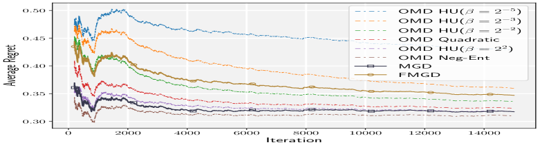
(a)

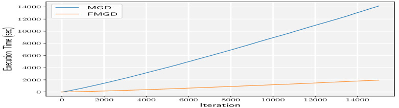
(b)

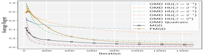
(c)

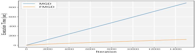
(d)

Figure 1: The top row and bottom row demonstrate experimental results for the proposed framework on simplex and $\mathbb{B}_{2}$, respectively. The details of experiments are described in Section 4.1.

5 Discussion and Future Work

In this paper, we have investigated the problem of finding the best algorithm among a class of OCO algorithms. To this end, we introduced a novel framework for OCO, based on the idea of employing expert advice and bandit as a master algorithm. As a special case, one can choose the family of optimizers based on the step size. In this case, the MetaGrad algorithm van Erven and Koolen (2016) can be recovered as a special case of our framework. Furthermore, we can choose the family of optimizers based on parameters about which we usually have no information such as Lipschitz constant, domain diameter, strong convexity coefficient, etc.  In this work, the family of OCO algorithms are considered to be finite. An interesting direction for future work would be to investigate the problem setup for a family of infinite algorithms. Moreover, we showed that partial and full feedback approaches maintain a trade-off between complexity and regret bound. As another potential direction for future work, one can consider the case of using feedback from more than one experts. From the enviornment’s point of view, we have studied the static regret. However, it should be emphasized that the dynamic regret Hall and Willett (2013); Jadbabaie et al. (2015); Mokhtari et al. (2016); Yang et al. (2016); Zhang et al. (2017) can be analyzed in the same fashion. Finally, to get the results of our experiments, stated in Section 4, we have used EXP3 in partial feedback setting. However, in practice we believe that employing algorithms more suitable for stochastic environment Bubeck et al. (2012) like Thompson sampling Russo et al. (2018) may lead to even better results.

Appendix A Background

In this section definition of Expert advice algorithm provided. After that Bregman Divergence definition, which is used in OMD algorithms, is provided. Then OMD algorithm and regret bound of it, is mentioned.

A.1 Expert Advice

On expert advice we have discussed but the framework and detailed algorithm of them are not provided. In this section some of algorithms in expert advice problem that we have used are introduced in detailed.

A.2 Framework

Expert advice framework:

Algorithm 4 Expert Advice

  Input: Learning rate $\eta>0$

  Initialization: Let $p_{1}$ be the distribution, according to the prior knowledge about experts

  for $t=1,\ldots,T$ do

     Get all experts predictions and play $a_{t}$ based on $p_{t}$ and predictions

     Observe losses of all experts as the vector $\ell_{t}$

     Update $p_{t+1}\in\Delta(K)$ based on losses we have observed so far

  end for

All of the below algorithms follow the above framework.

A.3 Squint

Squint algorithm is stated as bellow.

Algorithm 5 Squint Algorithm

  Input: learning rate $\eta>0$

  Initialization: let $R_{0},V_{0}$ be two all-zero vectors

  for t = 1, …, T do

     compute $p_{t}\in\Delta(K)$ such that $p_{t}(a)\propto p_{1}(i)exp(-\eta R_{t-1}(a))+\eta^{2}V_{t-1})$

     play $a_{t}\sim p_{t}$ and observe its loss vector $\ell_{t}$

     update $R_{t}=R_{t-1}+\ell_{t}$ and $\forall i:V_{t}(i)=V_{t-1}(i)+\ell_{t}(i)^{2}$

  end for

In fact in above algorithm, $R_{t}(a)$ denotes the expected regret w.r.t. $a$-th expert.

A.4 GBPA

GBPA algorithm is defined as bellow.

Algorithm 6 GBPA

  Input: learning rate $\eta>0$

  Initialization: let $\widehat{L}_{0}$ be the all-zero vector

  for t = 1, …, T do

     compute $p_{t}\in\Delta(K)$ such that $p_{t}\propto\nabla S_{\alpha}^{*}(-\frac{\widehat{L}_{t-1}}{\eta})$

     play $a_{t}\sim p_{t}$ and observe its loss $\ell_{t}(a_{t})$

     update $\widehat{L}_{t}=\widehat{L}_{t-1}+\widehat{\ell}_{t}$ where $\widehat{\ell}_{t}(a)=\frac{\ell_{t}(a)}{p_{t}(a)}\textbf{1}\{a=a_{t}\},\forall a\in[K]$

  end for

Above algorithm uses Tsallis entropy which is defined as below.

$$S_{\alpha}(L)=\frac{1}{1-\alpha}(1-\sum\limits_{i=1}^{K}L(i)^{\alpha})$$ (A.1)

EXP3 algorithm is GBPA where in (A.1) $\alpha\rightarrow 1$. Now we want to compute its update rule of probabilities for EXP3. By using L’Hôpital’s rule, we have

$$\lim\limits_{\alpha\rightarrow 1}S_{\alpha}(L)= \lim_{\alpha\rightarrow 1}\frac{(1-\sum_{i=1}^{K}L(i)^{\alpha})^{\prime}}{(1-\alpha)^{\prime}}$$

$$= \lim_{\alpha\rightarrow 1}\frac{\sum_{i=1}^{K}-\ln L(i)\cdot p_{i}^{\alpha}}{-1}$$

$$= \sum\limits_{i=1}^{K}\ln L(i)\cdot L(i)=H(L)$$

where $H(L)$ is negative entropy function. We know that $H^{*}(L)=\sup\limits_{x\in\mathbb{R}^{K}}(\left\langle L,x\right\rangle-H(x))$ so:

$$H^{*}(\frac{L}{\eta})=\frac{1}{\eta}\ln(\sum\limits_{i=1}^{K}\exp(\eta L(i)))$$

So $p_{t}(a)$ is the $a$-th element of $\nabla H^{*}(-\frac{\widehat{L}_{t-1}}{\eta})$ which is : $\frac{\exp(-\eta\widehat{L}_{t-1}(a))}{\sum_{i=1}^{K}\exp(-\eta\widehat{L}_{t-1}(i))}$. So EXP3 is defined by following algorithm.

Algorithm 7 EXP3

  Input: learning rate $\eta>0$

  Initialization: let $\widehat{L}_{0}$ be the all-zero vector

  for t = 1, …, T do

     compute $p_{t}\in\Delta(K)$ such that $p_{t}(a)\propto exp(-\eta\widehat{L}_{t-1}(a))$

     play $a_{t}\sim p_{t}$ and observe its loss $\ell_{t}(a_{t})$

     update $\widehat{L}_{t}=\widehat{L}_{t-1}+\widehat{\ell}_{t}$ where $\widehat{\ell}_{t}(a)=\frac{\ell_{t}(a)}{p_{t}(a)}\textbf{1}\{a=a_{t}\},\forall a\in[K]$

  end for

A.5 Bregman Divergence

Let $F\colon\mathcal{D}\subset\mathbb{R}^{d}\to\mathbb{R}$ be a strictly convex and differentiable function. Denote by $B_{F}(x,y)$ the Bregman divergence associated with $F$ for points $x,y$, defined by

$$B_{F}(x,y)\triangleq F(x)-F(y)-\left\langle\nabla F(y),x-y\right\rangle.$$ (A.2)

We also define the projection of a point $x\in\mathcal{D}$ onto a set $\mathcal{X}\subset\mathcal{D}$ with respect to $B_{F}$ as

$$\operatorname{\Pi}_{\mathcal{X}}^{F}(x)\triangleq\mathop{\mathrm{argmin}}_{z\in\mathcal{X}}B_{F}(z,x).$$

Here we give some useful property of the Bregman divergence.

Lemma A.1.

Let $F\colon\Delta(d)\to\mathbb{R}_{+}$ be the negative entropy function, defined as $F(x)=\sum_{i=1}^{d}x^{i}\log x^{i}$. Then, we have

$$B_{F}(x,y)=\mathrm{KL}(x\,\|\,y).$$ (A.3)

Moreover, if one extends the domain of $F$ to $\mathbb{R}_{+}^{d}$, then, defining the extended KL divergence as

$$\mathrm{KL}(x\,\|\,y)=\sum_{i=1}^{d}x^{i}\log\frac{x^{i}}{y^{i}}-(x^{i}-y^{i}),$$

the equality (A.3) holds.

A.6 Mirror Descent

The Online Mirror Descent (OMD) algorithm is defined as follows. Let $\mathcal{D}$ be a domain containing $\mathcal{X}$, and $\varphi\colon\mathcal{D}\to\mathbb{R}$ be a mirror map. Let $x_{1}=\mathop{\mathrm{argmin}}_{x\in\mathcal{X}}\varphi(x)$. For $t\geq 1$, set $y_{t+1}\in\mathcal{D}$ such that

$$\nabla\varphi(y_{t+1})=\nabla\varphi(x_{t})-\eta\nabla_{t},$$

and set

$$x_{t+1}=\operatorname{\Pi}_{\mathcal{X}}^{\varphi}(y_{t+1}).$$

Theorem A.2.

Let $\varphi\colon\mathcal{D}\to\mathbb{R}$ be a mirror map which is $\rho$-strongly convex w.r.t. a norm $\|\cdot\|$. Let $D=\sup_{x\in\mathcal{X}}B_{\varphi}(x,x_{1})$, and $f$ be convex and $L$-Lipschitz w.r.t. $\|\cdot\|$. Then, OMD with $\eta=\frac{\sqrt{2\rho D}}{L}\frac{1}{\sqrt{T}}$ gives

$$\mathcal{R}_{T}\leq L\sqrt{\frac{2DT}{\rho}}.$$ (A.4)

Note that if we did not have $T$, then if we set $\eta_{t}=\frac{\sqrt{2\rho D}}{L}\frac{1}{\sqrt{t}}$ we can achieve same regret bound.

Appendix B Analysis

Analysis of theorems and other materials in paper are stated in the following.

B.1 Auxiliary Lemmas

Lemma B.1.

Let $\mathcal{A}$ be an arbitrary expert advice algorithm, performs on expert set $\mathcal{M}$. Suppose that loss of our experts have upper bound $L$ instead of being in interval $[0,1]$. Then running $\mathcal{A}$ on normalized version of losses $\bar{\ell}_{t}=\frac{\ell_{t}}{L}$ gives following regret.

$$\mathcal{R}_{T}=L\mathcal{R}_{T}^{\mathcal{A}}$$

where $\mathcal{R}_{T}^{\mathcal{A}}$ is the regret for running algorithm $\mathcal{A}$ on normalized version of losses.

Proof.

If we play $a_{t}$ at iteration $t$ then we can write Regret of our proposed algorithm on bounded losses, we can say:

$$\mathcal{R}_{T}= \sum\limits_{t=1}^{T}\ell_{t}(a_{t})-\min\limits_{a\in\mathcal{M}}\sum\limits_{t=1}^{T}\ell_{t}(a)$$

$$= L\left(\sum\limits_{t=1}^{T}\bar{\ell}_{t}(a_{t})+\min\limits_{a\in\mathcal{M}}\sum\limits_{t=1}^{T}\bar{\ell}_{t}(a)\right)=L\mathcal{R}_{T}^{a}$$

∎

Lemma B.2.

Let cost functions $\{f_{t}\}_{t\in[T]}$ on domain $\mathcal{D}$ and tight upper bound for surrogate cost functions $F=\sup\limits_{x\in\mathcal{D},t\in[T]}|\left\langle\nabla_{t},x\right\rangle|$. Suppose that all $f_{t}$ are $L$-Lipschitz w.r.t. norm $\|.\|$ and $\mathcal{D}$ has upper bound $D$ w.r.t. norm $\|.\|$. Then $F\leq LD$.

Proof.

We know that if $f_{t}$ is $L$-Lipschitz w.r.t. norm $\|.\|$, then : $\|\nabla f_{t}(x)\|^{*}\leq L$. So by the Cauchy-Schwarz Inequality we have:

$$|\left\langle\nabla_{t},x\right\rangle| \leq\|\nabla_{t}\|^{*}\|x\|$$

$$\leq LD$$

So we have $F=\sup\limits_{x\in\mathcal{D},t\in[T]}|\left\langle\nabla_{t},x\right\rangle|\leq LD$ ∎

B.2 Proof of Proposition 3.1

Proof of Proposition 3.1.

Let $x^{*}=\arg\min\limits_{x\in\mathcal{D}}\sum\limits_{t=1}^{T}\left\langle\nabla_{t},x\right\rangle$ and $a^{*}=\arg\min\limits_{a\in[K]}\sum\limits_{t=1}^{T}\ell_{t}(a)$. Then for regret of our framework we have:

$$\mathcal{R}_{T} \leq\sum\limits_{t=1}^{T}f_{t}(x_{t})-\sum\limits_{t=1}^{T}f_{t}(x^{*})$$

$$\stackrel{{\scriptstyle\text{(a)}}}{{\leq}}\left\langle\nabla_{t},x_{t}-x^{*}\right\rangle$$

$$\stackrel{{\scriptstyle\text{(b)}}}{{=}}\sum\limits_{t=1}^{T}\left\langle\nabla_{t},x_{t}^{a_{t}}\right\rangle-\sum\limits_{t=1}^{T}\left\langle\nabla_{t},x_{t}^{a^{*}}\right\rangle+\sum\limits_{t=1}^{T}\left\langle\nabla_{t},x_{t}^{a^{*}}\right\rangle-\sum\limits_{t=1}^{T}\left\langle\nabla_{t},x^{*}\right\rangle$$

$$=2F\left(\sum\limits_{t=1}^{T}\ell_{t}(a_{t})-\sum\limits_{t=1}^{T}\ell_{t}(a^{*})\right)+\left(\sum\limits_{t=1}^{T}\widehat{f}_{t}(x_{t}^{a^{*}})-\sum\limits_{t=1}^{T}\widehat{f}_{t}(x^{*})\right)$$

$$=2F\mathcal{R}_{T}^{\mathcal{A}}+\mathcal{R}_{T}^{\mathsf{OCO}_{a^{*}}}$$

where (a) follows by convexity of $\{f_{t}\}_{t\in[T]}$ and (b) follows by the fact that $x_{t}=x_{t}^{a_{t}}$. ∎

B.3 Proof of Lemma 3.5

Proof of Lower Bound Lemma.

Consider an instance of OCO where $\mathcal{K}\subseteq\mathbb{R}^{d}$ is a ball with diameter $D$ w.r.t norm mentioned norm.

$$\mathcal{K}=\{x\in\mathbb{R}^{d}|\|x\|_{.}\leq D\}=D\{x|\|x\|\leq 1\}$$ (B.1)

Assume that $\bm{e}_{i}\in\mathbb{R}^{d}$ be the vector where all elements except $i$-th element are zero and the $i$-th element is $a_{i}>0$ such that $\|\bm{e}_{i}\|_{.}=1$. Define $V\triangleq\{L\bm{e}_{1},\ldots,L\bm{e}_{d},-L\bm{e}_{1},\ldots,-L\bm{e}_{d}\}$ be the set of $2d$ vectors with norm $L$. Now define $2d$ functions as bellow:

$$\forall~{}v\in V:f_{v}(x)=\left\langle v,x\right\rangle$$

The cost function in each iteration are chosen at random and uniformly from $\{f_{v}|v\in V\}$. So in iteration $t$ first algorithm $\mathcal{A}$ chooses $x_{t}$ and we choose random $v_{t}$ and incur cost function $f_{t}(x)=\left\langle v_{t},x\right\rangle$. Now we want to compute $\mathbb{E}(\mathcal{R}_{T})$.

$$\mathbb{E}(\mathcal{R}_{T})={} \mathbb{E}\left(\sum\limits_{t=1}^{T}f_{t}(x_{t})-\min\limits_{x\in\mathcal{K}}\sum\limits_{t=1}^{T}f_{t}(x)\right)$$

$$={} \sum\limits_{t=1}^{T}\mathbb{E}(\left\langle v_{t},x_{t}\right\rangle)-\mathbb{E}\left(\min\limits_{x\in\mathcal{K}}\sum\limits_{t=1}^{T}\left\langle v_{t},x\right\rangle\right)$$

$$\stackrel{{\scriptstyle\text{(a)}}}{{=}}{} \sum\limits_{t=1}^{T}\left\langle\mathbb{E}(v_{t}),\mathbb{E}(x_{t})\right\rangle)-\mathbb{E}\left(\min\limits_{x\in\mathcal{K}}\left\langle\sum\limits_{t=1}^{T}v_{t},x\right\rangle\right)$$

$$\stackrel{{\scriptstyle\text{(b)}}}{{=}}{} -\mathbb{E}\left(\min\limits_{x\in\mathcal{K}}\left\langle\sum\limits_{t=1}^{T}v_{t},x\right\rangle\right)$$

where (a) follows by the fact that $\{v_{t}\}_{t\in[T]}$ are i.i.d. and $x_{t}$ is depends on just $v_{1:t-1}$ so $x_{t},v_{t}$ are independent, (b) is due to $\mathbb{E}(v_{t})=0$. Now suppose that $S_{T}=\sum\limits_{t=1}^{T}v_{t}$ so we should compute $\mathbb{E}(\min\limits_{x\in\mathcal{K}}\left\langle S_{T},x\right\rangle)$. Since $\mathcal{K}$ is symmetric with respect to the origin, so for every vector $y\in\mathbb{R}^{d}$ we have $\max\limits_{x\in\mathcal{K}}\left\langle y,x\right\rangle=-\min\limits_{x\in\mathcal{K}}\left\langle y,x\right\rangle$, as a consequence we should calculate $\mathbb{E}(\max\limits_{x\in\mathcal{K}}\left\langle y,x\right\rangle)$. On the other hand we know that:

$$\max\limits_{x\in\mathcal{K}}\left\langle S_{T},x\right\rangle=\frac{D}{2}\max\limits_{\{x|\|x\|\leq 1\}}\left\langle S_{T},x\right\rangle=\frac{D}{2}\|S_{T}\|_{.}^{*}$$

So

$$\mathbb{E}(\mathcal{R}_{T})=\frac{D}{2}\mathbb{E}(\|S_{T}\|_{.}^{*})$$ (B.2)

Now we want to give a lower bound for $\|S_{T}\|_{.}^{*}$. Now we know that By the Cauchy-Schwarz inequality we can say that

$$\sum\limits_{i=1}^{d}a_{i}|S_{T}(i)| \leq\|S_{T}\|_{.}^{*}\|\bm{e}\|_{.}$$

$$\leq\|S_{T}\|_{.}^{*}\sum_{j=1}^{d}\|\bm{e}_{i}\|_{.}$$

$$=d\|S_{T}\|_{.}^{*}$$

where $\bm{e}(i)=sign(S_{T}(i))a_{i}$. So by using (B.8) we have:

$$\frac{D}{2d}\sum_{i=1}^{d}a_{i}\mathbb{E}(|S_{T}(i)|)\leq\mathbb{E}(\mathcal{R}_{T})$$ (B.3)

Now we know that $S_{T}(i)=\sum\limits_{t=1}^{T}v_{t}(i)$ and by considering i.i.d. property of $\{v_{t}\}_{t\in[T]}$, using central limit theorem result in $S_{T}(i)\simeq N(0,T\sigma^{2})$ where $\sigma^{2}=var(v_{t}(i))$ that is simply $\frac{L^{2}a_{i}^{2}}{d}$. Now it is sufficient to compute $\mathbb{E}(|S_{T}(i)|)$.

$$\mathbb{E}(|S_{T}(i)|)\simeq \frac{1}{\sqrt{2T\pi}\sigma}\int_{-\infty}^{\infty}|x|e^{\frac{-x^{2}}{2T\sigma^{2}}}dx$$

$$= \frac{\sqrt{2}}{\sqrt{T\pi}\sigma}\int_{0}^{\infty}xe^{\frac{-x^{2}}{2T\sigma^{2}}}dx$$

$$= \frac{-\sqrt{2T}\sigma e^{\frac{-x^{2}}{2T\sigma^{2}}}}{\sqrt{\pi}}|_{0}^{\infty}$$

$$= \frac{\sqrt{2T}La_{i}}{\sqrt{d\pi}}$$

So $\frac{D}{2d}\sum\limits_{i=1}^{d}a_{i}\mathbb{E}(|S_{T}(i)|)\simeq\frac{D}{2d}(\sum\limits_{i=1}^{d}a_{i}^{2})\frac{\sqrt{2T}L}{\sqrt{d\pi}}$ . Now using result (B.3) leads to having following bound:

$$\mathbb{E}(\mathcal{R}_{T})=\Omega(LD\sqrt{T})$$

This result show that there are sample vectors $\{\hat{v}_{t}\}_{t\in[T]}$ that regret of cost functions $\{f_{\hat{v}_{t}}\}_{t\in[T]}$ incurs $\Omega(LD\sqrt{T})$, anyway. ∎

Proof of Corollary 3.3.

Let $R_{T}$ be the random variable where obtained by Framework 1. Suppose $p_{t}$ be the probabilities over expert in round $t$. Then for regret bound of modified version of the framework we have:

$$\mathcal{R}_{T} =\sum\limits_{t=1}^{T}f_{t}(x_{t})-\min\limits_{x\in\mathcal{D}}\sum\limits_{t=1}^{T}f_{t}(x)$$

$$=\sum\limits_{t=1}^{T}f_{t}\left(\sum\limits_{i=1}^{K}x_{t}^{i}p_{t}(i)\right)-\sum\limits_{t=1}^{T}\min\limits_{x\in\mathcal{D}}f_{t}(x)$$

$$\stackrel{{\scriptstyle(a)}}{{\leq}}\sum\limits_{t=1}^{T}\sum\limits_{i=1}^{K}p_{t}(i)f_{t}(x_{t}^{i})-\min\limits_{x\in\mathcal{D}}\sum\limits_{t=1}^{T}f_{t}(x)$$

$$=\sum\limits_{t=1}^{T}\mathbb{E}(f_{t}(x_{t}^{i}))-\min\limits_{x\in\mathcal{D}}\sum\limits_{t=1}^{T}f_{t}(x)$$

$$=\mathbb{E}(R_{T})$$

where (a) follows by Jensen’s inequality. ∎

B.4 Proof of Theorem 3.6

Proof.

Proof of Theorem 3.6 Let $x^{*}=\arg\min\limits_{x\in\mathcal{D}}\sum\limits_{t=1}^{T}\left\langle\nabla_{t},x\right\rangle$ and $a$ is arbitrary optimizer in $[K]$. For the regret of this algorithm we can write:

$$\mathcal{R}_{T} \leq\sum\limits_{t=1}^{T}f_{t}(x_{t})-\sum\limits_{t=1}^{T}f_{t}(x^{*})$$ (B.4)

$$\stackrel{{\scriptstyle\text{(a)}}}{{\leq}}\left\langle\nabla_{t},x_{t}-x^{*}\right\rangle$$

$$\stackrel{{\scriptstyle\text{(b)}}}{{=}}\sum\limits_{t=1}^{T}\left\langle\nabla_{t},\sum\limits_{i=1}^{K}x_{t}^{i}p_{t}(i)\right\rangle-\sum\limits_{t=1}^{T}\left\langle\nabla_{t},x_{t}^{a}\right\rangle+\sum\limits_{t=1}^{T}\left\langle\nabla_{t},x_{t}^{a}\right\rangle-\sum\limits_{t=1}^{T}\left\langle\nabla_{t},x^{*}\right\rangle$$

$$=2F\left(\sum\limits_{t=1}^{T}(\left\langle p_{t},\ell_{t}\right\rangle-\ell_{t}(a))\right)+\left(\sum\limits_{t=1}^{T}\widehat{f}_{t}(x_{t}^{a})-\sum\limits_{t=1}^{T}\widehat{f}_{t}(x^{*})\right)$$

$$=2F\left(\sum\limits_{t=1}^{T}\mathbb{E}(\ell_{t}-\ell_{t}(a))\right)+\left(\sum\limits_{t=1}^{T}\widehat{f}_{t}(x_{t}^{a})-\sum\limits_{t=1}^{T}\widehat{f}_{t}(x^{*})\right)$$

$$=2F\mathbb{E}(\mathcal{R}_{T}^{\mathcal{A}})+\mathcal{R}_{T}^{\mathsf{OCO}_{a}}$$

where (a) follows by convexity of $\{f_{t}\}_{t\in[T]}$ and (b) follows by the fact that $x_{t}=\sum\limits_{i=1}^{K}x_{t}^{i}p_{t}(i)$.
By the Theorem 2.3 we have bound for $\mathbb{E}(\mathcal{R}_{T}^{\mathcal{A}})\leq 2\sqrt{V_{T}(i)\ln k}$. So we can rewrite (B.3) as following:

$$\mathcal{R}_{T} \leq 4F\sqrt{V_{T}(i)\ln K}+\mathcal{R}_{T}^{\mathsf{OCO}_{i}}\Rightarrow$$ (B.5)

$$\mathcal{R}_{T}\leq\min\limits_{i\in[K]}\left(4F\sqrt{V_{T}(i)\ln K}+\mathcal{R}_{T}^{\mathsf{OCO}_{i}}\right)$$

Suppose $a^{*}=\arg\min\limits_{i\in[K]}\mathcal{B}_{T}^{\mathsf{OCO}_{i}}$. By the assumption 3 that we had in Section 2 this algorithm $\mathsf{OCO}_{a^{*}}$ should perform on a family of $L$-Lipschitz cost functions and domains with diameter $D$, both w.r.t. some norm $\|.\|$. So by using Lemma 3.6 we can say that

$$\mathcal{B}_{T}^{\mathsf{OCO}_{a^{*}}} =\Omega(LD\sqrt{T})\Rightarrow$$ (B.6)

$$\sqrt{\ln K}\mathcal{B}_{T}^{\mathsf{OCO}_{a^{*}}} =\Omega(\sqrt{T\ln K}LD)$$

Using Lemma B.2 result in $F\leq LD$. Also we know that $V_{T}(i)=\sum\limits_{t=1}^{T}(\left\langle p_{t},\ell_{t}\right\rangle-\ell_{t}(i))^{2}$ and according to the fact that $\forall i:\ell_{t}(i)<1$ then we can bound $V_{T}(i)$ hence : $V_{T}(i)\leq T$. So we have:

$$4F\sqrt{V_{T}(i)\ln K}\leq 4\sqrt{\ln K}LD\sqrt{T}=\mathcal{O}(\sqrt{\ln K}LD\sqrt{T})$$ (B.7)

Now using (B.6) and (B.7), result in $4F\sqrt{V_{T}(i)\ln K}=\mathcal{O}\left(\sqrt{\ln K}\mathcal{B}_{T}^{\mathsf{OCO}_{a^{*}}}\right)$ and using Equation (B.5) leads to $\mathcal{R}_{T}=\mathcal{O}(\sqrt{\ln K}\mathcal{B}_{T}^{a^{*}})$. ∎

B.5 Proof of Theorem 3.10.

Proof of Theorem 3.10.

Let $x^{*}=\arg\min\limits_{x\in\mathcal{D}}\sum\limits_{t=1}^{T}\left\langle\nabla_{t},x\right\rangle$ and $i$ is arbitrary optimizer in $[K]$. As we mentioned in Proposition 3.2 for the regret of this algorithm we can write:

$$\mathcal{R}_{T}\leq 2F\mathcal{R}_{T}^{\mathcal{A}}+\mathcal{R}_{T}^{\mathsf{OCO}_{i}}$$ (B.8)

We have following upper bound for regret of $\mathsf{OCO}_{i}$.

$$\mathcal{R}_{T}^{\mathsf{OCO}_{i}}\leq\mathcal{B}_{T}^{\mathsf{OCO}_{i}}$$

So we can say that:

$$\mathbb{E}(\mathcal{R}_{T})\leq 2F\mathbb{E}(\mathcal{R}_{T}^{\mathcal{A}})+\mathcal{B}_{T}^{\mathsf{OCO}_{i}}$$

On the other hand, from Theorem 2.4, Corollary 2.5 and Lemma B.1 we have following regret bound for algorithm $\mathcal{A}$:

$$\alpha=1/2\ (GBPA):\mathbb{E}(\mathcal{R}_{T})\leq 8F\sqrt{TK},$$ (B.9)

$$\alpha\rightarrow 1\ (EXP3):\mathbb{E}(\mathcal{R}_{T})\leq 4F\sqrt{TK\ln K}$$

By the assumption 3 that we had in Section 2 this algorithm $\mathsf{OCO}_{i}$ should perform on a family of $L$-Lipschitz cost functions and domains with diameter $D$, both w.r.t. some norm $\|.\|$. So by using Lemma 3.6 we can say that

$$\mathcal{B}_{T}^{\mathsf{OCO}_{i}} =\Omega(LD\sqrt{T})$$ (B.10)

$$\Rightarrow\sqrt{K}\mathcal{B}_{T}^{\mathsf{OCO}_{i}} =\Omega(\sqrt{TK}LD),$$

$$\sqrt{K\ln K}\mathcal{B}_{T}^{\mathsf{OCO}_{i}} =\Omega(\sqrt{TK\ln K}LD)$$

Using Lemma B.2 result in $F\leq LD$. Combining (B.9), (B.10) and the fact that $F\leq LD$, result in :

$$\alpha=1/2\ (GBPA):\mathbb{E}(\mathcal{R}_{T})\leq\mathcal{O}(\sqrt{K}\mathcal{B}_{T}^{\mathsf{OCO}_{i}}),$$

$$\alpha\rightarrow 1\ (EXP3):\mathbb{E}(\mathcal{R}_{T})\leq\mathcal{O}(\sqrt{K\ln K}\mathcal{B}_{T}^{\mathsf{OCO}_{i}})$$

∎

B.6 Proof of Theorem 3.13

Proof.

According to Theorems 3.7 and 3.11 we have following bound for MGD and FMGD on the mentioned setting.

MGD: $$\mathcal{R}_{T}\leq 4F\sqrt{T\ln K}+\mathcal{B}_{T}^{\mathsf{OCO}_{i}},$$ (B.11)

FMGD: $$\mathbb{E}(\mathcal{R}_{T})\leq 8F\sqrt{TK}+\mathcal{B}_{T}^{\mathsf{OCO}_{i}}$$

Suppose that $d_{i}$ be diameter of $\mathcal{D}$ w.r.t. norm $\|.\|_{i}$. By strongly convexity of $\varphi_{i}$ we know that

$$B_{\varphi_{i}}(x,y)\geq\frac{1}{2}\rho_{i}\|x-y\|_{i}^{2}$$ (B.12)

$$\Rightarrow\sup\limits_{x,y\in\mathcal{D}}B_{\varphi_{i}}(x,y)\geq\sup\limits_{x,y\in\mathcal{D}}\frac{1}{2}\rho_{i}\|x-y\|_{i}^{2}$$

$$\Rightarrow D_{i}\geq\frac{1}{2}\rho_{i}d_{i}^{2}$$

Now by Lemma B.1 we have $F\leq L_{i}d_{i}$. So by using (B.12) we can see that: $F\leq L_{i}\sqrt{\frac{2D_{i}}{\rho_{i}}}$.
According to the fact that $\mathsf{OCO}_{i}$ is a OMD algorithm then by using A.2 leads to $\mathcal{B}_{T}^{\mathsf{OCO}_{i}}=L_{i}\sqrt{\frac{2D_{i}T}{\rho_{i}}}$ so by using these results and combining with (B.11) we have

MGD: $$\mathcal{R}_{T}\leq(4\sqrt{\ln K}+1)L_{i}\sqrt{\frac{2D_{i}T}{\rho_{i}}},$$

FMGD: $$\mathbb{E}(\mathcal{R}_{T})\leq(8\sqrt{K}+1)L_{i}\sqrt{\frac{2D_{i}T}{\rho_{i}}}$$

∎

Appendix C Domain Specific Example

The goal of this section is to examine the intrinsic difference between Quadratic and Negative Entropy regularizer, when the optimization domain is a $\Delta(d)$ and $\mathbb{B}_{2}$ Ball. Our goal in learning the best regularizer among family of regularizers, achieved by providing two main algorithm. We experimented these algorithms on two domains $\mathbb{B}_{2}$-Ball and $\Delta(d)$. In the following we want to find the best regularizer with two choices of regularizer for these domains, that can verify our experimental results on proposed algorithms. We study all four possible combinations in the following sections. Finally we will propose an regularizer function called Hypentropy that has parameter $\beta$ that tuning it leads to covering both Negative Entropy and Quadratic.

C.1 Computing Bregman Divergence

Negative Entropy is:

$$R(x)=\sum\limits_{i=1}^{d}x_{i}\log x_{i}$$

Quadratic is:

$$R(x)=\frac{1}{2}\|x\|_{2}^{2}$$

For Quadratic we have

$$B_{R}(x,y)=\frac{1}{2}\left\|x-y\right\|_{2}^{2}$$

and for Neg Entropy we have

$$B_{R}(x,y)=\sum_{i=1}^{d}y_{i}-\sum_{i=1}^{d}x_{i}+\sum_{i=1}^{d}x_{i}\log\frac{x_{i}}{y_{i}}$$

so we are going to compare these regularizers on two domain : $\Delta(d)$ and $\mathbb{B}_{2}$.

C.2 Quadratic Regularisation on $\mathbb{B}_{2}$

Let $R(x)=\frac{1}{2}\left\|x\right\|_{2}^{2}$ and $K=\left\{x:\left\|x-x_{0}\right\|_{2}\leq 1\right\}$ according to the definition of mirror descent algorithm we have:

$$y_{t+1}=x_{t}-\eta_{t}\nabla f(x_{t})$$

$$x_{t+1}=\operatorname{\Pi}_{K}^{R}(x_{t}-\eta_{t}\nabla f(x_{t}))=\frac{x_{t}-\eta_{t}\nabla f(x_{t})-x_{0}}{\left\|x_{t}-\eta_{t}\nabla f(x_{t})-x_{0}\right\|_{2}}+x_{0}$$

Analysis: using (A.4) we have the following bound:

$$\mathcal{R}_{T}\leq\mathcal{O}(L_{f,2}\sqrt{2T})$$

C.3 Entropic Regularization on $\mathbb{B}_{2}$

given that $R(x)=-\sum_{i=1}^{d}x_{i}log(x_{i})$ and $K=\left\{x:\left\|x-x_{0}\right\|_{2}\leq 1\right\}$ the projection using this norm seems not to have a simple analytical soloution and we can use numerical methods such as gradient descent.

Analysis: We know that $R(x)=-\sum_{i=1}^{d}|x_{i}|\log(|x_{i}|)$ is 1-strongly convex w.r.t. $\left\|.\right\|_{1}$. If we pick $x_{0}=\sqrt{d}^{-1}\bm{1}$ as a start point, to obtain the upper bound for regret we need to just calculate $D_{R}=\sup_{x\in K}B_{R}(x,x_{0})$ and bound $\left\|.\right\|_{\infty}$ with $\left\|.\right\|_{2}$ in order to compare with Quadratic regularizer regret bound.
First we provide bellow lemma:

Lemma C.1.

if $z_{i}\geq 0$ and $\sum_{i=1}^{d}z_{i}^{2}\leq c^{2}$ then $\sum_{i=1}^{d}z_{i}\log(z_{i})\leq c^{2}$

Proof.

It’s sufficient to consider the following inequality:

$$\forall z\in\mathbb{R}^{+}:\log z\leq z-1<z$$

∎

Assume that $y_{i}=|x_{i}|$ so we have the following bound on $D_{R}$ :

$$D_{R}=\underset{y\in K}{\sup}B_{R}(y,x_{0})= \sum_{i=1}^{d}y_{i}\log{y_{i}}+\sqrt{d}\log{\sqrt{d}}+\sum_{i=1}^{d}(\log{\sqrt{d}}-1)(y_{i}-\frac{1}{\sqrt{d}})$$

$$= \sum_{i=1}^{d}y_{i}\log{\frac{\sqrt{d}}{e}y_{i}}+\sqrt{d}(z_{i}:=\frac{\sqrt{d}}{e}y_{i},c:=\frac{\sqrt{d}}{e})$$

$$= \frac{\sum_{i=1}^{d}z_{i}\log{z_{i}}}{c}+\sqrt{d}\hskip 2.5pt\text{(Applying lemma \ref{lemma:ent})}$$

$$\leq c+\sqrt{d}=\frac{\sqrt{d}}{e}+\sqrt{d}=O(\sqrt{d})$$

For $\|.\|_{\infty}$ its easy to check that $\forall x\in\mathbb{R}^{d}$ :

$$\frac{\|x\|_{2}}{\sqrt{d}}\leq\|x\|_{\infty}\leq\|x\|_{2}$$ (C.1)

hence using equation (A.4) we have the following bound:

$$\mathcal{R}_{T}\leq O(L_{f,\infty}\sqrt{2D_{R}T})$$ (C.2)

Corollary C.2.

If our domain is unit ball ($\mathbb{B}_{2}$) then using quadratic regularizer gives us better regret bound comparing to negative entropy. To be more precise if we assume that upper bound for regret with respect to negative entropy and quadratic on $\mathbb{B}_{2}$ are $\mathcal{B}_{T}^{Ent}$ and $\mathcal{B}_{T}^{Quad}$, respectively, then we have the following inequality :

$$1\leq\frac{\mathcal{B}_{T}^{Ent}}{\mathcal{B}_{T}^{Quad}}\leq\sqrt{d}$$ (C.3)

C.4 Quadratic Regularisation on $\Delta(d)$

given that $R(x)=\frac{1}{2}\left\|x\right\|_{2}^{2}$ and

$$K=\left\{x=(x_{1},x_{2},...,x_{d})\in\mathbb{R}^{d}:\sum_{i=1}^{d}x_{i}=1,\forall i,1\leq i\leq d\right\}$$

first note that the projection onto the probability simplex using euclidean norm is very easy using KKT and you can see the following algorithm.

Euclidean projection of a vector onto the probability simplex

  Input: $y\in\mathbb{R}^{d}$

  Sort y into u:$u_{1}\geq u_{2}\geq...\geq u_{d}$

  Find $\rho$ = $\max\left\{1\leq j\leq d:u_{j}+\frac{1}{j}(1-\sum_{i=1}^{j}u_{i})>0\right\}$

  Define $\lambda$=$\frac{1}{\rho}(1-\sum_{i=1}^{\rho}u_{i})>0$

   Output: output x, s.t. $x_{i}=\max\left\{y_{i}+\lambda,0\right\}$

hence we have:

$$y_{t+1}=x_{t}-\eta_{t}\nabla f(x_{t})$$

$$x_{t+1}=\operatorname{\Pi}_{K}^{R}(x_{t}-\eta_{t}\nabla f(x_{t}))$$

and the projection is as we have defined above.

Analysis: It is easy to check that $D_{R}$ is constant. So by using (A.4) we have the following bound:

$$\mathcal{R}_{T}\leq O(L_{f,2}\sqrt{2T})$$ (C.4)

C.5 Entropic Regularisation on $\Delta(d)$

given that $R(x)=-\sum_{i=1}^{d}x_{i}\log(x_{i})$ and

$$K=\left\{x=(x_{1},x_{2},...,x_{d})\in\mathbb{R}^{d}:\sum_{i=1}^{d}x_{i}=1,\forall i,1\leq i\leq d\right\}$$

we can easily show that projection onto the $\Delta(d)$ using Bregman Divergence is like normalizing using L1-norm. Hence by the update rule of OMD we have

$$-1+\log(y_{t+1}^{(i)})=-1+\log(x_{t}^{(i)})-\eta_{t}\nabla f(x_{t}^{(i)})$$

so:

$$y_{t+1}^{(i)}=x_{t}^{(i)}\exp(-\eta_{t}\nabla f(x_{t}^{(i)}))$$

$$x_{t+1}^{(i)}=\operatorname{\Pi}_{K}^{R}(x_{t}^{(i)}\exp(-\eta_{t}\nabla f(x_{t}^{(i)})))=\frac{x_{t}^{(i)}\exp(-\eta_{t}\nabla f(x_{t}^{(i)}))}{\sum_{i=1}^{d}x_{t}^{(i)}\exp(-\eta_{t}\nabla f(x_{t}^{(i)}))}$$

Analysis: pick $x_{0}=d^{-1}1$ and $R(x)=-\sum_{i=1}^{d}x_{i}\log(x_{i})$ is 1-strongly convex w.r.t. $\left\|.\right\|_{1}$ . Then

$$\underset{x\in K}{\sup}B_{R}(x,x_{0})=\underset{x\in K}{\sup}KL(x,x_{0})=\log(d)+\underset{x\in K}{\sup}\sum_{i=1}^{d}x_{i}\log(x_{i})\leq\log(d)$$

hence using (A.4) we have the following bound:

$$\mathcal{R}_{T}\leq\mathcal{O}(L_{f,\infty}\sqrt{2\log(d)T})$$ (C.5)

Corollary C.3.

If our domain is $\Delta(d)$ then based on equations C.1, C.4 and C.5 we can compare regret bound of two regularizers (Quadratic and negative entropy) on this domain :

$$\frac{1}{\sqrt{\log d}}\leq\frac{\mathcal{B}_{T}^{Quad}}{\mathcal{B}_{T}^{Ent}}\leq\sqrt{\frac{d}{\log d}}$$ (C.6)

So we can say that based on Lipschitzness of our functions sometimes negative entropy has better performance than quadratic and sometimes vise versa. But our intuition tell us that equation C.1 on average is near the lower bound instead of upper bound and as consequence the lower bound of above corollary can be substitute with 1 which result in better performance of negative entropy than quadratic on $\Delta(d)$.

C.6 Hypentropy

Here we introduce a regularizer that covers both negative entropy and quadratic norm.

Definition C.4.

(Hyperbolic-Entropy) For all $\beta>0$, let $\phi_{\beta}\colon\mathbb{R}^{d}\to\mathbb{R}$ be defined as:

$$\phi_{\beta}(x)=\sum_{i=1}^{d}x_{i}\arcsin(\frac{x_{i}}{\beta})-\sqrt{x_{i}^{2}+\beta^{2}}$$ (C.7)

The Bregman divergence is a measure of distance between two points defines in term of strictly convex function and here for hypentropy function $\phi_{\beta}$ is driven like below:

$$B_{\phi}(x,y)=\phi_{\beta}(x)-\phi_{\beta}(y)-\langle\nabla\phi_{\beta}(x),(x-y)\rangle$$ (C.8)

$$=\sum_{i=1}^{d}[x_{i}(\arcsin(\frac{x_{i}}{\beta})-\arcsin(\frac{y_{i}}{\beta}))-\sqrt{x_{i}^{2}+\beta^{2}}+\sqrt{y_{i}^{2}+\beta^{2}}]$$

The key reason that makes this function behave like both euclidean distance and relative entropy is that the hessian of hypentropy would be interpolate between hessian of both functions while vary parameter $\beta$ from 0 to $\infty$.

First we calculate the hessian of $\phi_{\beta}$ to compare it to Euclidean distance and entropy function:

$$\phi_{\beta}^{\prime\prime}(x)=\frac{1}{\sqrt{x^{2}+\beta^{2}}}$$

Now consider $x\ll\beta$ then $\phi_{\beta}^{\prime\prime}(x)=\frac{1}{\beta}$ is constant function similar to euclidean distance and in other case consider $\beta=0$ then $\phi_{\beta}^{\prime\prime}(x)=\frac{1}{|x|}$ and it is the same as hessian of negative entropy.

C.6.1 Diameter calculations for hypentropy

In this section we calculate the diameter for both $\Delta(d)$ and $\mathbb{B}_{2}$

First we need good approximation for bregman divergence of hypentropy function:

$$B_{\phi}(x,0)=\phi_{\beta}(x)-\phi_{\beta}(0)$$

$$=\sum_{i=1}^{d}(x_{i}\arcsin(\frac{x_{i}}{\beta})-\sqrt{x_{i}^{2}+\beta^{2}})+\beta d$$

$$\leq\sum_{i=1}^{d}x_{i}\arcsin(\frac{x_{i}}{\beta})$$

$$=\sum_{i=1}^{d}|x_{i}|\log(\frac{1}{\beta}(\sqrt{x_{i}^{2}+\beta^{2}}+|x_{i}|))$$

Thus WLOG,

$$\mathrm{diam}(\mathbb{B}_{2})\leq\sum_{i=1}^{d}x_{i}\log(\frac{1}{\beta}(\sqrt{x_{i}^{2}+\beta^{2}}+x_{i}))$$

$$\leq\sum_{i=1}^{d}x_{i}\log(1+\frac{2x_{i}}{\beta})$$

$$\leq\sum_{i=1}^{d}\frac{2x_{i}^{2}}{\beta}=\frac{2\|x\|_{2}^{2}}{\beta}\leq\frac{2}{\beta}$$

For $\Delta(d)$ if consider $\beta\leq 1$ this inequality holds, $\sqrt{x_{i}^{2}+\beta^{2}}+x_{i}\leq\sqrt{2}+1<3$. thus, it is clear that:

$$\mathrm{diam}(\Delta(d))<\sum_{i=1}^{d}x_{i}\log(\frac{3}{\beta})=\|x\|_{1}\log(\frac{3}{\beta})=\log(\frac{3}{\beta})$$

and if $\beta\geq 1$ also we have, $\sqrt{x_{i}^{2}+\beta^{2}}+x_{i}\leq\beta\sqrt{1+(\frac{x_{i}}{\beta})^{2}}+x_{i}\leq\sqrt{2}\beta+1$. Hence, in this case we have:

$$\mathrm{diam}(\Delta(d))\leq\sum_{i=1}^{d}x_{i}\log(\frac{\sqrt{2}\beta+1}{\beta})\leq\sum_{i=1}^{d}x_{i}\log(\sqrt{2}+1)=\|x\|_{1}\log(\sqrt{2}+1)<\log(3)$$

References

- Abernethy et al. (2015) Jacob D Abernethy, Chansoo Lee, and Ambuj Tewari. Fighting bandits with a new kind of smoothness. In Advances in Neural Information Processing Systems, pages 2197–2205, 2015.
- Auer et al. (2002a) Peter Auer, Nicolo Cesa-Bianchi, Yoav Freund, and Robert E Schapire. The nonstochastic multiarmed bandit problem. SIAM journal on computing, 32(1):48–77, 2002a.
- Auer et al. (2002b) Peter Auer, Nicolo Cesa-Bianchi, and Claudio Gentile. Adaptive and self-confident on-line learning algorithms. Journal of Computer and System Sciences, 64:48–75, 2002b.
- Bubeck et al. (2012) Sebastien Bubeck, Nicolo Cesa-Bianchi, et al. Regret analysis of stochastic and nonstochastic multi-armed bandit problems. Foundations and Trends® in Machine Learning, 5(1):1–122, 2012.
- Cesa-Bianchi and Lugosi (2006) Nicolo Cesa-Bianchi and Gabor Lugosi. Prediction, Learning, and Games. Cambridge University Press, New York, NY, USA, 2006.
- Cutkosky and Boahen (2017) Ashok Cutkosky and Kwabena Boahen. Online learning without prior information. arXiv preprint arXiv:1703.02629, 2017.
- Duchi et al. (2011) John Duchi, Elad Hazan, and Yoram Singer. Adaptive subgradient methods for online learning and stochastic optimization. Journal of Machine Learning Research, 12(Jul):2121–2159, 2011.
- Freund and Schapire (1997) Yoav Freund and Robert E Schapire. A decision-theoretic generalization of on-line learning and an application to boosting. Journal of computer and system sciences, 55(1):119–139, 1997.
- Ghai et al. (2019) Udaya Ghai, Elad Hazan, and Yoram Singer. Exponentiated gradient meets gradient descent. arXiv preprint arXiv:1902.01903, 2019.
- Hall and Willett (2013) Eric C Hall and Rebecca M Willett. Dynamical models and tracking regret in online convex programming. arXiv preprint arXiv:1301.1254, 2013.
- Hazan et al. (2007) Elad Hazan, Amit Agarwal, and Satyen Kale. Logarithmic regret algorithms for online convex optimization. Machine Learning, 69(2-3):169–192, 2007.
- Hazan et al. (2016) Elad Hazan et al. Introduction to online convex optimization. Foundations and Trends® in Optimization, 2(3-4):157–325, 2016.
- Jadbabaie et al. (2015) Ali Jadbabaie, Alexander Rakhlin, Shahin Shahrampour, and Karthik Sridharan. Online optimization: Competing with dynamic comparators. In Artificial Intelligence and Statistics, pages 398–406, 2015.
- Koolen and Van Erven (2015) Wouter M Koolen and Tim Van Erven. Second-order quantile methods for experts and combinatorial games. In Conference on Learning Theory, pages 1155–1175, 2015.
- Littlestone and Warmuth (1994) Nick Littlestone and Manfred K Warmuth. The weighted majority algorithm. Information and computation, 108(2):212–261, 1994.
- McMahan and Streeter (2010) H Brendan McMahan and Matthew Streeter. Adaptive bound optimization for online convex optimization. arXiv preprint arXiv:1002.4908, 2010.
- Mokhtari et al. (2016) Aryan Mokhtari, Shahin Shahrampour, Ali Jadbabaie, and Alejandro Ribeiro. Online optimization in dynamic environments: Improved regret rates for strongly convex problems. In 2016 IEEE 55th Conference on Decision and Control (CDC), pages 7195–7201. IEEE, 2016.
- Russo et al. (2018) Daniel J Russo, Benjamin Van Roy, Abbas Kazerouni, Ian Osband, Zheng Wen, et al. A tutorial on thompson sampling. Foundations and Trends® in Machine Learning, 11(1):1–96, 2018.
- Shalev-Shwartz et al. (2012) Shai Shalev-Shwartz et al. Online learning and online convex optimization. Foundations and Trends® in Machine Learning, 4(2):107–194, 2012.
- van Erven and Koolen (2016) Tim van Erven and Wouter M Koolen. Metagrad: Multiple learning rates in online learning. In Advances in Neural Information Processing Systems, pages 3666–3674, 2016.
- Vovk (1998) Vladimir Vovk. A game of prediction with expert advice. Journal of Computer and System Sciences, 56(2):153–173, 1998.
- Vovk (1990) Volodimir G Vovk. Aggregating strategies. Proc. of Computational Learning Theory, 1990, 1990.
- Yang et al. (2016) Tianbao Yang, Lijun Zhang, Rong Jin, and Jinfeng Yi. Tracking slowly moving clairvoyant: optimal dynamic regret of online learning with true and noisy gradient. In Proceedings of the 33rd International Conference on International Conference on Machine Learning-Volume 48, pages 449–457. JMLR. org, 2016.
- Zhang et al. (2017) Lijun Zhang, Tianbao Yang, Jinfeng Yi, Jing Rong, and Zhi-Hua Zhou. Improved dynamic regret for non-degenerate functions. In Advances in Neural Information Processing Systems, pages 732–741, 2017.