At What Level Should One Cluster Standard Errors in Paired and Small-Strata Experiments?

Abstract

In matched-pairs experiments in which one cluster per pair of clusters is assigned to treatment, to estimate treatment effects, researchers often regress their outcome on a treatment indicator and pair fixed effects, clustering standard errors at the unit-of-randomization level. We show that even if the treatment has no effect, a 5%-level $t$-test based on this regression will wrongly conclude that the treatment has an effect up to 16.5% of the time. To fix this problem, researchers should instead cluster standard errors at the pair level. Using simulations, we show that similar results apply to clustered experiments with small strata.

In this paper, we show that a statistical test commonly used by researchers analyzing a certain type of randomized controlled trials (RCTs) has a much larger error rate than previously thought. We then suggest a simple fix.

The type of RCTs this paper applies to are clustered RCTs with large clusters, meaning that there are more than 10 observations per randomization unit, and where the treatment is assigned within pairs of units, or within small strata of less than 10 units. For instance, our paper would apply to an RCT where the researcher pairs some villages, randomly assigns one village per pair to the treatment, and estimates a regression at the villager rather than at the village level, with more than 10 villagers per village. Our paper would also apply to an RCT where the researcher groups villages into small strata of six villages and randomly assigns two villages per pair to the treatment. While such paired or small-strata RCTs with large clusters do not account for the majority of RCTs conducted in economics, it seems that they are still fairly common. We surveyed the universe of published editions of the American Economic Journal: Applied Economics (AEJ Applied) from 2014 to 2018, and found that this type of RCT represents 20% of the RCTs published by the journal during that period.

In paired or small-strata RCTs with large clusters, researchers usually estimate the treatment effect by regressing their outcome on the treatment and pair or stratum fixed effects, “clustering” their standard errors at the unit-of-randomization level, namely, at the village level in our example. Then, they typically use the 5%-level $t$-test based on this regression to assess if the treatment has an effect. As any statistical test, this $t$-test may lead them to commit a type 1 error: even if the treatment does not have an effect, this $t$-test may lead them to wrongly conclude that the treatment has an effect. When using a 5%-level test, researchers hope that the probability that this would happen, the so-called error rate of the test, is less than 5%. We show that the error rate of this $t$-test may in fact be much larger than the researcher’s 5% target.

We start by considering paired RCTs with large clusters. There, we show that even if the treatment has no effect, this 5%-level $t$-test will wrongly conclude that the treatment has an effect up to 16.5% of the time, an error rate more than three times larger than the targeted one. We then show that to achieve the desired 5% error rate, researchers should instead cluster their standard errors at the pair level. Finally, we revisit 371 regressions from the paired RCTs in our survey, and find that clustering at the pair rather than at the randomization-unit level diminishes the number of effects that are significant at the 5% level by one third.

The intuition underlying our results is rather simple. In regression analysis, clustered standard errors are reliable when the regression’s dependent and independent variables are uncorrelated across clusters (Cameron and Miller, 2015). Therefore, in a paired RCT, clustering at the unit level relies on the assumption that the regression’s independent variable, the treatment, is uncorrelated across all randomization units. However, the treatments of the two units in the same pair are perfectly negatively correlated: if unit A is treated, then unit B must be untreated, and vice versa. This is the reason why unit-clustered standard errors are unreliable, and the error rate of the $t$-test based on unit-clustered standard errors differs from that targeted by the researcher. On the other hand, clustering at the pair level only relies on the assumption that units’ treatments are uncorrelated across pairs, which is true by design in paired experiments. This is the reason why pair-clustered standard errors are reliable, and the error rate of the $t$-test based on pair-clustered standard errors is equal to the error rate targeted by the researcher.

Our recommendations apply only to paired and clustered RCTs with large clusters. If the RCT is nonclustered, the 5%-level $t$-test based on unit-clustered standard errors has a 5% error rate, as targeted, after the degrees-of-freedom (DOF) adjustment automatically implemented in most statistical software. On the other hand, after this DOF adjustment the error rate of the 5%-level $t$-test based on pair-clustered standard errors is lower than 5%. Therefore, to achieve their targeted error rate in nonclustered paired RCTs, researchers should either use DOF-adjusted unit-clustered standard errors, or non-DOF-adjusted pair-clustered standard errors. In clustered RCTs, the same applies to regressions estimated at the unit-of-randomization level rather than at the observation level. Finally, in clustered RCTs with strictly fewer than 10 observations per randomization unit, our recommendation is to use pair-clustered standard errors, without the DOF adjustment. Figure 1 below summarizes our recommendations for applied researchers, depending on whether their RCT is clustered and on the number of observations per randomization unit.

Then, we turn to small-strata RCTs with large clusters. Using simulations, we show that our results for paired designs extend to this case. Intuitively, there as well the treatments of units in the same stratum are negatively correlated, so this correlation should be accounted for. Therefore, our simulations show that in those designs too, the error rate of the 5%-level $t$-test based on unit-clustered standard errors is larger than 5%. The difference between the $t$-test’s actual and targeted error rates diminishes when the number of units per strata increases. Again, this makes intuitive sense: the larger the strata, the lower the correlation of the treatments of units belonging to the same stratum. For instance, with five units per strata, the error rate of the 5% level $t$-test based on unit-clustered standard errors is equal to 7.9%. With 10 units per strata, this error rate is equal to 6.2%. With more than 10 units per strata, this error rate is lower than 6%, and becomes very close to the targeted 5% error rate. This is why, though we acknowledge it is somewhat arbitrary, we use a threshold of 10 units per strata to define an RCT with “small” strata. Our simulations also show that the error rate of the 5%-level $t$-test based on strata-clustered standard errors is very close to 5%. Accordingly, in small-strata RCTs with large clusters, we recommend that researchers cluster their standard errors at the strata level. If the RCT has too few strata to cluster at that level, researchers could use randomization inference, or the standard-error estimator in Section 9.5.1 of Imbens and Rubin (2015), provided each stratum has at least two treated and two control units.

Related literature

Our paper is related to several papers that predate ours. Imai, King and Nall (2009) show that, when units all have the same number of observations, pair-clustered standard errors are reliable in clustered and paired RCTs. With respect to their paper, we show that this result still holds when units have varying numbers of observations, thus justifying pair-level clustering under more realistic assumptions. Moreover, while they focus on finite-sample results, we present large-sample results for $t$-tests based on pair-clustered standard errors.

Bruhn and McKenzie (2009) use simulations to study, in nonclustered paired RCTs, the error rate of a $t$-test without clustering, which is equivalent to unit-clustering when the RCT is nonclustered. They show that this error rate is equal to the targeted error rate. This result may appear to conflict with ours, but this apparent discrepancy comes from the DOF adjustment embedded in most statistical software. In nonclustered RCTs, the regression with pair fixed effects has one fixed effect for each pair of observations. Accordingly, it has approximately half as many regressors as observations, so the DOF adjustment amounts to multiplying nonclustered standard errors by approximately $\sqrt{2}$, which, we show, makes them almost equivalent to the non-DOF-adjusted pair-clustered standard errors. This is why the error rate of DOF-adjusted nonclustered $t$-tests is equal to the targeted error rate in nonclustered paired RCTs.

Abadie et al. (2017) examine the appropriate level of clustering in regression analysis. They define a cluster as a group of units whose treatments are positively correlated. Their results apply to the case where the assignment is fully clustered (all units in the same cluster have the same treatment), and to the case where the assignment is probabilistically clustered (units in the same cluster have positively correlated treatments). Their Corollary 1 states that standard errors need to account for clustering whenever units’ treatments are positively clustered within clusters. Our results are consistent with theirs. The main difference is that we consider a case in which units’ treatments are negatively correlated within clusters (the pairs in our paper), which is not something they consider. However, our papers share a common theme: that standard errors need to account for clustering when treatments are correlated within some groups of units.

Athey and Imbens (2017) and Bai, Romano and Shaikh (2021) study the error rate of $t$-tests based on unit-clustered standard errors in paired experiments, when pair fixed effects are not included in the regression. They both show that without pair fixed effects, the test’s error rate is lower than the targeted error rate. We instead show that when pair fixed effects are included in the regression, the error rate of this test becomes larger than the targeted error rate. In our survey of paired experiments, we find that including pair fixed effects in the regression is a much more common practice than not including those fixed effects.

The rest of this paper is organized as follows. Section 2 presents our survey of paired and small-strata RCTs in economics. Section 3 introduces our main theoretical results. Section 4 presents our simulation study. Section 5 presents our empirical application. Section 6 briefly discusses various extensions of our baseline results, which are fully developed in our Online Appendix. Section 7 concludes. Throughout the paper, a unit refers to a randomization unit (e.g., a village), while an observation refers to the level at which the regression is estimated (e.g., a villager).

1 Survey of Paired and Small-Strata Experiments in Economics

We searched the 2014–2018 issues of the AEJ Applied for clustered and paired RCTs, and for clustered and stratified RCTs with 10 or fewer units per strata. 50 field-RCT papers were published over that period. Three RCTs were clustered and relied on a paired randomization for all of their analysis. One RCT was clustered and relied on a paired randomization for part of its analysis. Seven RCTs were clustered and used a stratified design with, on average, 10 or fewer units per strata. 10 of those 11 RCTs have, on average, more than 10 observations per randomization unit, while one stratified RCT has 5.8 observations per randomization unit. Overall, 11 (22%) of the 50 field RCTs published by the AEJ Applied over that period are clustered paired or small-strata RCTs, and 10 (20%) also have large clusters.

To increase our sample of paired RCTs, we also searched the AEA’s registry website (https://www.socialscienceregistry.org). We looked at all completed projects, whose randomization method includes the word “pair” and that either have a working or a published paper. We conducted that search on January 9th, 2019, and found four more clustered and paired RCTs. All of them have, on average, more than 10 observations per randomization unit. Combining our two searches, we found 15 clustered paired or small-strata RCTs. The list is in Table LABEL:tab:litrev in the Online Appendix.

We now give descriptive statistics on our sample of RCTs. Across the eight paired RCTs, the median number of pairs is 27, the median number of observations per unit is 112, and units have on average more than 10 observations in all RCTs. To estimate the treatment effect, six articles include pair fixed effects in all their regressions, one article includes pair fixed effects in some but not all their regressions, and one article does not include pair fixed effects in any regression. All articles cluster standard errors at the unit level.

Across the seven small-strata RCTs, the median number of units per strata is 7, the median number of strata is 48, the median number of observations per unit is 26, and units have more than 10 observations on average in all but one RCT. To estimate the treatment effect, six articles include stratum fixed effects in all their regressions, and one article does not include stratum fixed effects in any regression. All articles cluster standard errors at the unit level.

In the following sections, we focus on paired RCTs. In Section LABEL:se:ext_small_strata of the Online Appendix, we use simulations to show that the main results we derive for paired RCTs extend to small-strata RCTs.

2 Theoretical Results

2.1 Setup

We consider a population of $2P$ units. Unlike Abadie and Imbens (2008) and Bai, Romano and Shaikh (2021), we do not assume that the units are an independent and identically distributed (i.i.d.) sample drawn from a superpopulation. Instead, that population is fixed, and its characteristics are not random. Our survey suggests that this modeling framework, similar to that in Neyman (1923) and Abadie et al. (2020), is applicable to the majority of paired- and small-strata RCTs in our survey. Units are drawn from a larger population in only one of those fifteen RCTs. In all the other RCTs, the sample is a convenience sample, consisting of volunteers to receive the treatment, or of units located in areas where conducting the research was easier. When the units are an i.i.d. sample drawn from a super-population, our results still hold, conditional on the sample.

The $2P$ units are matched into $P$ pairs. Pairs are created by grouping together units with the closest value of some baseline variables predicting the outcome. In our fixed-population framework, pairing is not random, as it depends on fixed units’ characteristics. The pairs are indexed by $p\in\{1,\dots,P\}$, and the two units in pair $p$ are indexed by $g\in\{1,2\}$. Unit $g$ in pair $p$ has $n_{gp}$ observations, so that pair $p$ has $n_{p}=n_{1p}+n_{2p}$ observations, and the population has $n=\sum_{p=1}^{P}n_{p}$ observations. When $n_{gp}>1$ for at least some units, the RCT is clustered; when $n_{gp}=1$ for all units, the RCT is nonclustered.

Treatment is assigned as follows. For all $p\in\{1,\dots,P\}$ and $g\in\{1,2\}$, let $W_{gp}$ be an indicator variable equal to 1 if unit $g$ in pair $p$ is treated, and to 0 otherwise. We assume that the treatments satisfy the following conditions.

Assumption 1 (Paired assignment)

1. For all $p$, $W_{1p}+W_{2p}=1$.

2. $\mathbb{P}(W_{gp}=1)=\frac{1}{2}$ for all $g$ and $p$.

3. $(W_{1p},W_{2p})_{p=1}^{P}$ is jointly independent across $p$.

Point 1 requires that in each pair, one of the two units is treated. Point 2 requires that the two units have the same probability of being treated. Point 3 requires that the treatments be independent across pairs. Assumption 1 is typically satisfied by design in paired experiments.

Let $y_{igp}(1)$ and $y_{igp}(0)$ represent the potential outcomes of observation $i$ in unit $g$ and pair $p$ with and without the treatment, respectively. We follow the randomization-inference literature (see Abadie et al., 2020) and assume that potential outcomes are fixed. The observed outcome is $Y_{igp}=y_{igp}(1)W_{gp}+y_{igp}(0)(1-W_{gp})$. Our target parameter is the average treatment effect (ATE)

$$\tau=\frac{1}{n}\sum_{p=1}^{P}\sum_{g=1}^{2}\sum_{i=1}^{n_{gp}}[y_{igp}(1)-y_{igp}(0)].$$

We consider two estimators of $\tau$. The first estimator $\widehat{\tau}$ is the OLS estimator from the regression of the observed outcome $Y_{igp}$ on a constant and $W_{gp}$:

(1) $$Y_{igp}=\widehat{\alpha}+\widehat{\tau}W_{gp}+\epsilon_{igp}\qquad i=1,2,\dots,n_{gp};\ g=1,2;\ p=1,\dots,P.$$

The second estimator is the pair-fixed-effects estimator, $\widehat{\tau}_{fe}$, obtained from the regression of the observed outcome $Y_{igp}$ on $W_{gp}$ and a set of pair fixed effects $(\delta_{ig1},\dots,\delta_{igP})$:

(2) $$Y_{igp}=\widehat{\tau}_{fe}W_{gp}+\sum_{p=1}^{P}\widehat{\gamma}_{p}\delta_{igp}+u_{igp},\qquad i=1,\dots,n_{gp};\ g=1,2;\ p=1,\dots,P.$$

2.2 Properties of Unit- and Pair-Clustered Variance Estimators

We study the variance estimators of $\widehat{\tau}$ and $\widehat{\tau}_{fe}$, when the regression is clustered at either the pair level or the unit level. The clustered-variance estimators we study are those proposed in Liang and Zeger (1986). Lemma C.1 in Online Appendix C gives simple expressions of $\widehat{\mathbb{V}}_{pair}(\widehat{\tau})$ and $\widehat{\mathbb{V}}_{pair}(\widehat{\tau}_{fe})$, the pair-clustered variance estimators (PCVEs) of $\widehat{\tau}$ and $\widehat{\tau}_{fe}$, and of $\widehat{\mathbb{V}}_{unit}(\widehat{\tau})$ and $\widehat{\mathbb{V}}_{unit}(\widehat{\tau}_{fe})$, the unit-clustered variance estimators (UCVEs) of $\widehat{\tau}$ and $\widehat{\tau}_{fe}$.

We now present our main results, that are derived under the following assumption.

Assumption 2

There is a strictly positive integer $N$ such that for all $p$, $n_{1p}=n_{2p}=N$.

Assumption 2 requires that all units have the same number of observations. Let

$$\widehat{\tau}_{p}=\sum_{g}\left[W_{gp}\frac{1}{n_{gp}}\sum_{i}Y_{igp}-(1-W_{gp})\frac{1}{n_{gp}}\sum_{i}Y_{igp}\right]$$

denote the difference between the average outcome of treated and untreated observations in pair $p$. Under Assumption 2, one can show that

$$\widehat{\tau}=\widehat{\tau}_{fe}=\sum_{p=1}^{P}\frac{\widehat{\tau}_{p}}{P},$$

that both estimators are unbiased for the ATE, and that

(3) $$\mathbb{V}(\widehat{\tau})=\mathbb{V}(\widehat{\tau}_{fe})=\frac{1}{P^{2}}\sum_{p=1}^{P}\mathbb{V}(\widehat{\tau}_{p}).$$

Let $\tau_{p}\equiv\frac{1}{n_{p}}\sum_{g=1}^{2}\sum_{i=1}^{n_{gp}}[y_{igp}(1)-y_{igp}(0)]$ be the ATE in pair $p$. For all $d\in\{0,1\}$, let $\overline{y}_{gp}(d)\equiv\frac{1}{n_{gp}}\sum_{i}y_{igp}(d)$, $\overline{y}_{p}(d)\equiv\frac{1}{2}\sum_{g}\overline{y}_{gp}(d)$, and $\overline{y}(d)\equiv\sum_{p}\overline{y}_{p}(d)/P$, respectively, denote the average outcome with treatment $d$ in pair $p$’s unit $g$, in pair $p$, and in the entire population.

Lemma 2.1

1. If Assumptions 1 and 2 hold, then $\widehat{\mathbb{V}}_{pair}(\widehat{\tau})=\widehat{\mathbb{V}}_{pair}(\widehat{\tau}_{fe})$, and

   $$\operatorname{\mathbb{E}}\left[\frac{P}{P-1}\widehat{\mathbb{V}}_{pair}(\widehat{\tau})\right]=\mathbb{V}(\widehat{\tau})+\frac{1}{P(P-1)}\sum_{p=1}^{P}(\tau_{p}-\tau)^{2}\geq\mathbb{V}(\widehat{\tau}).$$

2. If Assumption 2 holds, then $\widehat{\mathbb{V}}_{pair}(\widehat{\tau})=2\widehat{\mathbb{V}}_{unit}(\widehat{\tau}_{fe})$.

3. If Assumptions 1 and 2 hold, then

   $$\operatorname{\mathbb{E}}\left[\frac{P}{P-1}\left(\widehat{\mathbb{V}}_{unit}(\widehat{\tau})-\widehat{\mathbb{V}}_{pair}(\widehat{\tau})\right)\right] =\frac{2}{P}\left(\frac{1}{P-1}\sum_{p}\left(\overline{y}_{p}(0)-\overline{y}(0)\right)\left(\overline{y}_{p}(1)-\overline{y}(1)\right)\right.$$

   $$\left.-\frac{1}{P}\sum_{p}\sum_{g}\frac{1}{2}\left(\overline{y}_{gp}(0)-\overline{y}_{p}(0)\right)\left(\overline{y}_{gp}(1)-\overline{y}_{p}(1)\right)\right).$$

Proof 2.2.

See Online Appendix A.

Point 1 of Lemma 2.1 shows that the PCVEs without and with pair fixed effects are equal, and that after a DOF correction, their expectation is at least as large as the variance of $\widehat{\tau}$. If the treatment effect is heterogeneous across pairs, $\frac{1}{P(P-1)}\sum_{p=1}^{P}(\tau_{p}-\tau)^{2}>0$ so the inequality is strict: the PCVEs are upward-biased estimators for the variance of $\widehat{\tau}$. If the treatment effect does not vary across pairs, the inequality becomes an equality: the PCVEs are unbiased for the variance of $\widehat{\tau}$. Building upon Point 1 of Lemma 2.1, in the Online Appendix we show that when the number of pairs grows, $(\widehat{\tau}-\tau)/\widehat{\mathbb{V}}_{pair}(\widehat{\tau})$ and $(\widehat{\tau}_{fe}-\tau)/\widehat{\mathbb{V}}_{pair}(\widehat{\tau}_{fe})$, the $t$-statistics of the difference-in-means and fixed-effects estimators using the PCVEs, both converge to a normal distribution with a mean equal to 0 and a variance lower than 1 in general, but equal to 1 when the treatment effect is homogenous across pairs (see Point 1 of Theorem B.1). Comparing those $t$-statistics to critical values of a standard normal leads to a test with an error rate at most equal to the researcher’s target. For instance, if the average treatment effect $\tau$ is equal to zero, by comparing $\left|\widehat{\tau}/\sqrt{\widehat{V}_{pair}(\widehat{\tau})}\right|$ to 1.96, one would wrongly conclude that $\tau\neq 0$ at most 5% of the time, as desired.

On the other hand, Point 2 of Lemma 2.1 shows that the UCVE with pair fixed effects is equal to a half of the PCVEs. Combined with Point 1 of Lemma 2.1, this implies that the UCVE with pair fixed effects may severely underestimate the variance of $\widehat{\tau}$: if the treatment effect is constant across pairs, its expectation is equal to half of the variance of $\widehat{\tau}$. Building upon Point 2 of Lemma 2.1, in the Online Appendix we show that when the number of pairs grows, $(\widehat{\tau}_{fe}-\tau)/\widehat{\mathbb{V}}_{unit}(\widehat{\tau}_{fe})$, the $t$-statistic of the fixed-effects estimator using the UCVE, converges to a normal distribution with a mean equal to 0 and a variance twice as large as that of the $t$-statistic using the PCVE (see Point 2 of Theorem B.1). Therefore, comparing that $t$-statistic to critical values of a standard normal may yield a test with a substantially larger error rate than the researcher’s target. For instance, if the average treatment effect $\tau$ is equal to zero and the treatment effect is homogenous across pairs, by comparing $\left|\widehat{\tau}_{fe}/\sqrt{\widehat{V}_{unit}(\widehat{\tau}_{fe})}\right|$ to 1.96, one would wrongly conclude that $\tau\neq 0$ 16.5% of the time, an error rate more than three times larger than the researcher’s target.

With heterogeneous treatment effects across pairs, the error rates of the $t$-tests using the PCVEs may be lower than the researcher’s target, while the error rate of the $t$-test using the UCVE with pair fixed effects may be equal to that target. However, in practice we do not know if the treatment effect is constant or heterogeneous, and it is common to require that a test have an error rate no larger than some target uniformly across all possible data-generating processes. The $t$-tests using the PCVEs satisfy that property, unlike the $t$-test using the UCVE with pair fixed effects.

Finally, Point 3 of Lemma 2.1 shows that without pair fixed effects, the expectation of the difference between the UCVE and PCVE is proportional to the difference between the between-pair and within-pair covariance of the two potential outcomes. In most applications, both terms should be positive, as the two potential outcomes should be positively correlated. One may also expect the difference between those two terms to be positive, as units in the same pair should have more similar potential outcomes than units in different pairs. For instance, in the extreme case where units in the same pair have equal potential outcomes, the second term is equal to 0. Consequently, the expectation of the difference between the UCVE and the PCVE should often be positive. Then, it follows from Point 1 of Lemma 2.1 that the UCVE without pair fixed effects is a more upward-biased estimator of the variance of $\widehat{\tau}$ than the PCVEs, and that it remains upward-biased even if the treatment effect is constant across pairs. Finally, building upon Point 3 of Lemma 2.1, in the Online Appendix we show that the error rate of the $t$-statistic of the difference-in-means estimator using the UCVE is lower and further away from the researcher’s target than the error rate of the $t$-test making use of the PCVEs (see Point 3 of Theorem B.1).

Intuitively, the UCVEs are biased because clustering at the unit level does not account for the perfect negative correlation of the treatments of the two units in the same pair. Cluster-robust standard errors rely on the assumption that observations’ outcomes and treatments are uncorrelated across clusters (see Cameron and Miller, 2015). This assumption is violated when one clusters at the unit level, but it holds when one clusters at the pair level.

The direction of the bias of the UCVE depends on whether pair fixed effects are included in the regression. When pair fixed effects are not included in the regression, the UCVE will in general overestimate the variance of $\widehat{\tau}$. This result may be relatively intuitive. With positive correlations between observations, as is often the case with time-series data, the variance of an estimator is usually larger than what it would be without those correlations. Then, one would expect that negative correlations would reduce an estimator’s variance. This is indeed what we find in Point 3 of Lemma 2.1: the UCVE, which estimates $\widehat{\tau}$’s variance as if the treatments of two units in the same pair were not negatively correlated, is larger than needed.

On the other hand, when pair fixed effects are included in the regression, the UCVE may underestimate the variance of $\widehat{\tau}$. This result is less intuitive. It comes from the fact that with pair fixed effects in the regression, the sample residuals $u_{igp}$ are by construction uncorrelated with the pair fixed effects, which implies that for every $p$, the sum of the residuals in pair $p$ is zero:

$$\sum_{i,g}u_{igp}=0.$$

Splitting the summation between $g=1$ and $g=2$, using the fact that under Assumption 2 units 1 and 2 have the same number of observations, and letting $\overline{u}_{g,p}$ denote the average residuals of observations in unit $g$ of pair $p$, the previous display implies that $\overline{u}_{1,p}=-\overline{u}_{2,p}$, which in turn implies that $\left(\overline{u}_{1,p}\right)^{2}=\left(\overline{u}_{2,p}\right)^{2}$: by construction, the squares of the average residuals are equal in the treated and control units of each pair. Now, one can show that with pair fixed effects, the UCVE is proportional to

$$\frac{1}{(2P)^{2}}\sum_{p=1}^{P}\sum_{g=1}^{2}\left(\overline{u}_{g,p}\right)^{2},$$

the sum, across all units, of their average squared residuals, divided by the number of units squared. Accordingly, $\widehat{\mathbb{V}}_{unit}(\widehat{\tau}_{fe})$ treats $\left(\overline{u}_{1,p}\right)^{2}$ and $\left(\overline{u}_{2,p}\right)^{2}$ as if they were independent to estimate the variance of $\widehat{\tau}_{fe}$, while they are equal to each other. Instead, the PCVE is proportional to

$$\frac{1}{P^{2}}\sum_{p=1}^{P}\left(\overline{u}_{1,p}\right)^{2}.$$

$\widehat{\mathbb{V}}_{pair}(\widehat{\tau}_{fe})$ uses only one squared-residual per pair to estimate the variance of $\widehat{\tau}_{fe}$.

As Section 4 below shows, our recommendation of using the PCVE rather than the UCVE in clustered-paired RCTs and regressions with pair fixed effects leads to a significant reduction in the number of effects that are significant at the 5% level in the published papers we revisit. One may then wonder whether our results contradict those in Bai (2019), who shows that pairing is the optimal RCT design to maximize statistical precision. The short answer is that our findings do not contradict his important result. Bai (2019) shows that the RCT design that minimizes $\mathbb{V}(\widehat{\tau})$, and therefore the mean-squared error of $\widehat{\tau}$, is a specific paired design. We do not derive any new result on $\mathbb{V}(\widehat{\tau})$, so our results have no bearing on his. Instead, our main result is to show that $\widehat{\mathbb{V}}_{unit}(\widehat{\tau}_{fe})$, a commonly used variance estimator in paired experiments, can be severely downward-biased. Instead, we recommend using another estimator, $\widehat{\mathbb{V}}_{pair}(\widehat{\tau}_{fe})$, that is not downward biased, and leads to a $t$-test with an error rate no larger than the researcher’s target when the treatment does not have an effect. Using $\widehat{\mathbb{V}}_{pair}(\widehat{\tau}_{fe})$ instead of $\widehat{\mathbb{V}}_{unit}(\widehat{\tau}_{fe})$, researchers will conclude less often that the treatments they consider have an effect, but comparing the power of those two $t$-tests is not a fair comparison: the former test has an error rate no larger than the researcher’s target when the treatment does not have an effect, unlike the latter one. Overall, while paired RCTs may not be as powerful as the use of a spuriously-low variance estimator had led researchers to believe, they remain a very powerful RCT design, the one that leads to the lowest mean-squared error of $\widehat{\tau}$.

There is only one case where our results could imply that other designs might be preferable to paired RCTs, though further research is needed to validate or invalidate this conjecture. In our simulations, we find that with fewer than 20 pairs, $t$-tests based on the PCVE become less reliable: with fewer than 40 units, using the PCVE in paired RCTs may lead to invalid inference. Thus, it may be preferable to run a more coarsely stratified RCT with at least four units per strata, and use, for example, the variance estimator proposed in Section 6.1 of Athey and Imbens (2017) for stratified RCTs. However, to our knowledge, the validity of this alternative inference procedure has not been assessed yet with a small number of units in the RCT. Note that in the (admittedly small) sample of eight paired RCTs in our survey, one has five pairs and another one has 14 pairs. All the other RCTs are close to the 20-pair “threshold” (one has 19 pairs), or above it. Accordingly, while paired RCTs with far fewer than 20 pairs are not a rarity, they do not seem to be common either.

2.3 Accounting for Degrees-of-Freedom Adjustments

The clustered-variance estimators we study are those proposed in Liang and Zeger (1986). Typically, statistical software report DOF-adjusted versions of those estimators. For instance, in Stata the default adjustment is to multiply the Liang and Zeger estimator by $[(n-1)/(n-k)]\times[G/(G-1)]$, where $n$ is the sample size, $k$ the number of regressors, and $G$ the number of clusters (see StataCorp, 2017). This DOF adjustment is implemented when one uses the regress or areg command, not when one uses the xtregress command (see Cameron and Miller, 2015). In R, if the researcher uses the sandwich package, the default DOF adjustment when declaring a cluster variable is the same as in Stata, namely, $[(n-1)/(n-k)]\times[G/(G-1)]$. $G/(G-1)$ is close to $1$, so the important term in the DOF adjustment is $(n-1)/(n-k)$.

In regressions without pair fixed effects, there are only two regressors (the constant and the treatment), so $(n-1)/(n-k)=(n-1)/(n-2)$. This quantity is close to 1, so the DOF adjustment leaves the UCVE and the PCVE almost unchanged. Accordingly, in regressions without pair fixed effects, the guidance we derived in the previous section also applies to the DOF-adjusted UCVE and PCVE: the former estimator should not be used, while the latter estimator can be used.

On the other hand, in regressions with pair fixed effects, the DOF adjustment may affect the UCVE and the PCVE more substantially. When the paired RCT is not clustered, the regression has $2P$ observations and $P+1$ regressors, so $(n-1)/(n-K)=(2P-1)/(P-1)\approx 2:$ the DOF-adjusted UCVE is twice as large as the non-DOF-adjusted UCVE. This fact and Point 2 of Lemma 3 imply that in nonclustered RCTs, the DOF-adjusted UCVE with pair fixed effects is almost equal to the non-DOF-adjusted PCVE with pair fixed effects and has the same desirable properties. On the other hand, the DOF-adjusted PCVE with pair fixed effects is now about twice as large as the non-DOF-adjusted PCVE with pair fixed effects, so this estimator is upward-biased even under constant treatment effect. Overall, in nonclustered paired RCTs and regressions with pair fixed effects, the guidance we derived in the previous section no longer applies to the DOF-adjusted UCVE and PCVE: the former estimator can be used, while the latter estimator should not be used.

When the paired RCT is clustered and the regression has pair fixed effects, the regression has $2P\overline{n}_{u}$ observations and $P+1$ regressors, where $\overline{n}_{u}$ denotes the average number of observations across all units. Accordingly, $(n-1)/(n-K)=(2P\overline{n}_{u}-1)/(2P\overline{n}_{u}-(P+1))\approx 2\overline{n}_{u}/(2\overline{n}_{u}-1).$ This quantity is decreasing in $\overline{n}_{u}$: the larger the average number of observations across units, the smaller the DOF adjustment. Simulations shown in Panel D of Table 1 show that with $\overline{n}_{u}=5$, the error rate of a $t$-test based on the DOF-adjusted UCVE is still considerably larger than the researcher’s target: unlike what happens in nonclustered experiments, the DOF-adjustment is not sufficient to ensure the error rate of this $t$-test is equal to the researcher’s target. The same panel also shows that with $\overline{n}_{u}=5$, the error rate of a $t$-test based on the DOF-adjusted PCVE is slightly below the researcher’s target, even under constant treatment effects. When $\overline{n}_{u}=10$, simulations shown in Panel C of Table 1 show that the error rate of a $t$-test based on the DOF-adjusted PCVE is now very close to the researcher’s target. Overall, in clustered paired RCTs with more than 10 observations per unit, the guidance we derived in the previous section also applies to the DOF-adjusted UCVE and PCVE: the former estimator should not be used, while the latter estimator can be used. In clustered paired RCTs with strictly fewer than 10 observations per unit, we recommend using the PCVE without the DOF adjustment, which is in line with a recommendation in Cameron and Miller (2015) in a different context. In Stata, the xtregress command computes this estimator.

2.4 Should Pair Fixed Effects Be Included in the Regression?

Though this paper is primarily concerned with the estimation of the variance of treatment effect estimators, our recommendations crucially depend on whether pair fixed effects are included in the regression. In this section, we discuss the pros and cons of including such pair fixed effects. (Our paper does not bring any new result to this longstanding discussion; we rely on earlier results, sometimes specializing them to the case of paired RCTs.)

In nonclustered experiments, or in clustered experiments where in each pair the two randomization units have the same number of observations ($n_{1p}=n_{2p}$ for all $p$), if no randomization unit attrits from the sample, adding pair fixed effects to the regression leaves the treatment coefficient unchanged: $\widehat{\tau}=\widehat{\tau}_{fe}$. Because $\widehat{\tau}$ and $\widehat{\tau}_{fe}$ are equal, their variances are also equal: adding pair fixed effects to the regression does not lead to any precision gain in nonclustered paired experiments or in clustered experiments where in each pair the two randomization units have the same number of observations. When there is attrition, $\widehat{\tau}$ and $\widehat{\tau}_{fe}$ will differ: $\widehat{\tau}_{fe}$ will only leverage observations from pairs where both randomization units are observed, while $\widehat{\tau}$ will also leverage observations from pairs where only one of the randomization units is observed. King et al. (2007) argue in favor of dropping pairs with one attriting unit, while Bai (2019) shows they can be kept. At any rate, even if one would prefer to drop those pairs, one can simply do so before running the regression, rather than running the regression with pair fixed effects in the full sample. Overall, in nonclustered experiments, or in clustered experiments where in each pair the two randomization units have the same number of observations, there is no strong argument for or against adding pair fixed effects to the regression.

In clustered experiments where there are pairs where the two randomization units have different numbers of observations ($n_{1p}\neq n_{2p}$ for some $p$), adding pair fixed effects to the regression may change the treatment coefficient: $\widehat{\tau}\neq\widehat{\tau}_{fe}$. In such cases, one can show that $\widehat{\tau}$, the standard difference in means estimator, converges toward our target parameter $\tau$, the average treatment effect, when the number of pairs goes to infinity. $\widehat{\tau}_{fe}$ on the other hand does not converge toward $\tau$: one can show that it converges toward a parameter that has sometimes been called a variance weighted average (see Angrist and Pischke, 2008) of the average treatment effect in each pair. This parameter may differ from $\tau$ if the treatment effect varies across pairs. Accordingly, unlike $\widehat{\tau}$, $\widehat{\tau}_{fe}$ may be biased for $\tau$, even asymptotically. On the other hand, the variance of $\widehat{\tau}_{fe}$ is often lower than that of $\widehat{\tau}$ (see Imai, King and Nall, 2009). Overall, if one is primarily interested in consistently estimating $\tau$, pair fixed effects should not be included in the regression. If one wants to use the most precise estimator, pair fixed effects should be included in the regression.

Figure 1 summarizes our recommendations for practitioners, regarding whether pair fixed effects should be included in the regression, and regarding which variance estimator one should use.

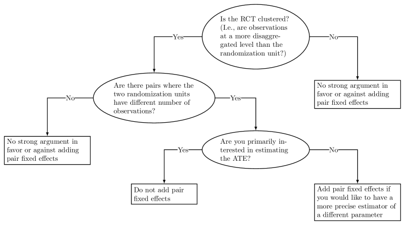
(a) Decision 1: Should the regression include pair fixed effects? (See Section 3.4 for more details.)

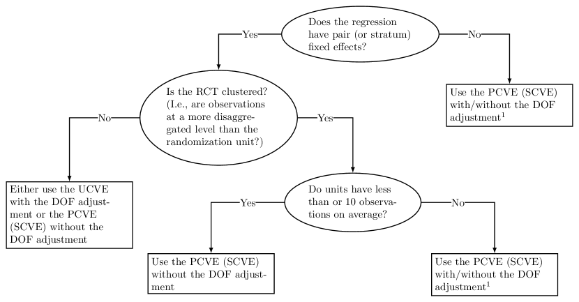
(b) Decision 2: Which variance estimator should one use? (See Section 3.3 for more details.)

Figure 1: Recommendations for Practitioners

UCVE = unit-clustered variance estimators. PCVE = pair-clustered variance estimators. DOF = degrees of freedom. In these cases, the PCVE with and without the DOF adjustment are very similar.

3 Simulations Using Real Data

We perform Monte-Carlo simulations using a real data set. We use the data from the microfinance RCT in Crépon et al. (2015b). The authors matched 162 Moroccan villages into 81 pairs, and in each pair, they randomly assigned one village to a microfinance treatment. They sampled households from each village and measured their outcomes such as their credit access and income. The number of observations varies substantially across units: the average number of villagers per village is 34.1, with a standard deviation of 9.2, a minimum of 13 and a maximum of 58.

In the paper, the authors report the effect of the microfinance intervention on 82 outcome variables. For each outcome, we construct potential outcomes assuming no treatment effect, i.e., $y_{igpk}(0)=y_{igpk}(1)=Y_{igpk}$, where $Y_{igpk}$ is the value of outcome $k$ for villager $i$ in village $g$ and pair $p$. We then simulate 1000 treatment assignments $W_{k}^{j}=((W_{11,k}^{j},W_{21,k}^{j}),\dots,(W_{1P,k}^{j},W_{2P,k}^{j}))$, assigning one of the two villages to treatment in each pair. Then, we regress $Y_{igpk}$ on the simulated treatment. We estimate regressions with and without pair fixed effects, clustering at the pair level and at the village level. Thus, we obtain four $t$-statistics, and four 5% level $t$-tests. Importantly, those $t$-tests are based on Stata’s regress command, so they make use of DOF-adjusted variance estimators. The estimated error rate of each $t$-test is the percentage of times, across the 82,000 regressions (82 outcomes $\times$ 1000 simulations), that the $t$-statistic is greater in absolute value than 1.96, meaning that the test leads the researcher to wrongly conclude that the treatment has an effect. Because the data is generated with a constant treatment effect of zero, these error rates should be equal to 5% if the tests are valid.

Column (1) of Panel A of Table 1 shows the results using the authors’ actual data set, with 81 pairs and villages’ actual number of villagers. The error rates of the $t$-tests using pair-clustered variance estimators (PCVEs) are close to 5%, irrespective of whether pair fixed effects are included in the regression. On the other hand, when the unit-clustered variance estimator (UCVE) is used with pair fixed effects, the error rate of the $t$-test is equal to 17.4%, very close to the 16.5% error rate predicted by Point 2 of Theorem B.1. Finally, the error rate of the $t$-test with the UCVE and no pair fixed effects is equal to 1.4%, well below 5%. Columns (2), (3), and (4) show that we obtain similar results if we use a random sample of 40, 30, and 20 pairs. With fewer than 20 pairs, the PCVE becomes downward-biased. One may then have to use randomization inference tests.

Panel B (resp. C) of Table 1 shows the error rates of the four $t$-tests, in a data set where villages all have 20 (resp. 10) villagers. In each village, the villagers are a random sample from the village’s population, that does not vary across simulations. Results are similar to Panel A.

Panel D shows the error rates of the four $t$-tests, in a data set where villages all have 5 villagers. Again, the error rate of the $t$-test with the PCVE and no pair fixed effects is close to 5%. On the other hand, the error rate of the $t$-test with the PCVE and pair fixed effects is now below 5%. As discussed in Section 2.3, this is due to the fact that the DOF-adjustment is not negligible anymore with 5 villagers per village. The error rate of the $t$-test with the UCVE and pair fixed effects is still much higher than 5%, but less so than in Panel A. Finally, the error rate of the $t$-test with the UCVE and no pair fixed effects is still well below 5%, though less so than in Panel A. These simulations justify the guidance above: in clustered RCTs with strictly fewer than 10 observations per unit, one should either use the PCVE without pair fixed effects, with or without the DOF adjustment, or the PCVE with pair fixed effects without the DOF adjustment.

Finally, Panel E of Table 1 shows the error rates of the four $t$-tests, in a data set where a quarter of the villages have five villagers, a quarter have 10 villagers, a quarter have 20 villagers, and a quarter have their actual number of villagers. In Columns (1) and (2), results are fairly similar to those in Panel A. In Columns (3) and (4), the error rates of the $t$-tests using the PCVEs are larger than 5% (though much less so than the $t$-test using the UCVE with pair fixed effects). This is related to the results in Carter, Schnepel and Steigerwald (2017), who find that when clusters have very heterogeneous sizes, one needs a larger number of clusters to ensure that asymptotic distributions yield accurate approximations of the finite-sample distribution of cluster-robust $t$-statistics. Note that this phenomenon is absent in Panel A, while village sizes are already fairly heterogeneous in those simulations. In applications where units have very heterogeneous numbers of observations, researchers may need to perform their own simulations to assess whether $t$-tests using the PCVEs can be used.

Table 1: Error Rates of $T$-tests, in Simulations Based on Crépon et al. (2015a)

Clustering level	Pair Fixed Effects	5% level $t$-test error rate
		With 81 pairs (1)	With 40 pairs (2)	With 30 pairs (3)	With 20 pairs (4)
Panel A: Actual village sizes
pair	Yes	0.0515	0.0519	0.0527	0.0559
pair	No	0.0527	0.0540	0.0541	0.0572
unit	Yes	0.1704	0.1742	0.1802	0.1840
unit	No	0.0137	0.0171	0.0178	0.0192
Panel B: All villages have 20 villagers
pair	Yes	0.0464	0.0508	0.0510	0.0537
pair	No	0.0491	0.0540	0.0541	0.0562
unit	Yes	0.1663	0.1692	0.1741	0.1737
unit	No	0.0161	0.0210	0.0190	0.0259
Panel C: All villages have 10 villagers
pair	Yes	0.0432	0.0439	0.0464	0.0454
pair	No	0.0489	0.0503	0.0538	0.0498
unit	Yes	0.1575	0.1581	0.1622	0.1686
unit	No	0.0214	0.0238	0.0249	0.0265
Panel D: All villages have 5 villagers
pair	Yes	0.0360	0.0384	0.0371	0.0363
pair	No	0.0480	0.0514	0.0502	0.0477
unit	Yes	0.1393	0.1372	0.1367	0.1421
unit	No	0.0287	0.0281	0.0313	0.0284
Panel E: Heterogeneous village sizes
pair	Yes	0.0517	0.0543	0.0597	0.0673
pair	No	0.0567	0.0571	0.0623	0.0692
unit	Yes	0.1701	0.1716	0.1775	0.1797
unit	No	0.0180	0.0231	0.0228	0.0271

The table reports the error rates of four 5% level $t$-tests in Crépon et al. (2015a). For each of the 82 outcomes in the paper, we randomly drew 1000 simulated treatment assignments, following the paired assignment used by the authors, and regressed the outcome on the simulated treatment. The four $t$-tests are computed, respectively, without and with pair fixed effects in the regression, and clustering standard errors at the village or at the pair level. All $t$-tests are based on Stata’s regress command, so they make use of DOF-adjusted variance estimators. The error rate of each test is the percent of times, across the 82,000 regressions (82 outcomes $\times$ 1000 replications), that the test leads the researcher to wrongly conclude that the treatment has an effect. Column (1) (resp. (2), (3), (4)) shows the results using the original sample of 81 pairs (resp. a fixed sample of 40, 30, 20 randomly selected pairs). In Panel A, villages all have their actual number of villagers. In Panel B (resp. C, D), each village has 20 (resp. 10, 5) villagers, that are a fixed random sample from the village’s population. In Panel E, 1/4 of villages have 5 villagers, 1/4 have 10 villagers, 1/4 have 20 villagers, and 1/4 have their actual number of villagers.

4 Application

In this section, we revisit the paired RCTs in our survey. The data used in four of those papers is publicly available (Beuermann et al., 2015b; Bruhn et al., 2016b; Crépon et al., 2015b; Glewwe, Park and Zhao, 2016b). Those four papers used a clustered RCT, and all have more than 10 observations per randomization unit (across the four papers, the lowest average number of observations per randomization unit is 21.5). The authors estimated the effect of the treatment in 294 regressions, clustering at the unit level. In Panel A of Table 2, we re-estimate those regressions, clustering at the pair level, and including the same controls as the authors. In the 240 regressions with pair fixed effects, the average of the unit-clustered variance estimator (UCVE) divided by the pair-clustered variance estimator (PCVE) is equal to 0.548. The UCVE divided by the PCVE is not always exactly equal to 1/2, because Assumption 2 is not always satisfied, but these fractions all are quite close to 1/2, as predicted by Lemma LABEL:le:ext_fe in the Online Appendix. The authors originally found that the treatment has a 5%-level significant effect in 110 regressions. Using the PCVE, we find significant effects in just 74 regressions. In the 54 regressions without pair fixed effects, the UCVE is on average 1.18 times larger than the PCVE. The authors originally found 31 significant effects, we find 36 significant effects using the PCVE.

The data used in the remaining four papers is not publicly available. Three of those papers estimated 131 regressions with pair fixed effects, clustering standard errors at the unit level. For those regressions, we multiply the UCVE by the average value of of the PCVE divided by the UCVE found in Panel A of Table 2 to predict the value of the PCVE. Panel B of Table 2 shows that while the authors originally found a 5%-level significant effect in 51 regressions, we find significant effects in just 34 regressions. The fourth paper estimated regressions only without pair fixed effects. Because without fixed effects, the value of the PCVE divided by the UCVE can vary significantly across regressions, we do not try to predict the PCVEs of that paper.

Table 2: Using Unit- or Pair-Level Clustered Variance Estimators in Paired RCTs

	Unit-level divided by pair-level clustered variance estimators	Number of 5%-level significant effects with UCVE	Number of 5%-level significant effects with PCVE	Number of Regressions
Panel A: Articles with publicly available data
with pair fixed effects	0.548	110	74	240
without pair fixed effects	1.184	31	36	54
Panel B: Articles without publicly available data
with pair fixed effects		51	34	131

The table shows the effect of using pair-clustered variance estimators (PCVE) rather than unit-level clustered variance estimators (UCVE) in seven of the paired RCTs we found in our survey. In Panel A, we consider four papers whose data is available online, and re-estimate their regressions clustering standard errors at the pair level. Column 1 shows the ratio of the unit- and pair-level clustered variance estimators, separately for regressions without and with pair fixed effects. Column 2 (resp. 3) shows the number of 5%-level significant effects using unit- (resp. pair-) clustered standard errors. In Panel B, we consider three other papers whose data is not available online, and use the average ratio of the unit- and pair- clustered variance estimators found in Panel A to predict the value of the pair-clustered estimator in the regressions with pair fixed effects estimated by those papers. Column 2 (resp. 3) shows the number of 5%-level significant effects using unit- (resp. predicted pair-) clustered standard errors.

5 Extensions

In our Online Appendix, we consider various extensions. In Appendix LABEL:se:ext_small_strata, we present simulations showing that our results for paired RCTs extend to stratified RCTs with few units per strata.

Assumption 2, which requires that all units have the same number of observations, allows us to derive the stark results in Lemma 2.1. Under Assumption 2, $\widehat{\tau}$ and $\widehat{\tau}_{fe}$ are equal, but the UCVE drastically changes when one adds pair fixed effects to the regression. This is obviously undesirable: the two estimators are equal, their variances are equal, so their variance estimators should not be drastically different. In practice, however, Assumption 2 often fails. In that case, we show in Section LABEL:sec:ext_assm2 of the Online Appendix that our main conclusions still hold. Without that assumption, the PCVEs remain upward-biased in general and unbiased if the treatment effect is homogeneous across pairs. On the other hand, the UCVE with pair fixed effects may still be downward-biased. Specifically, Point 2 of Lemma 2.1 still holds if the number of observations per unit varies across pairs, as long as the two units in a pair have the same number of observations. If the number of observations per unit varies within pairs, Point 2 of Lemma 2.1 still approximately holds, unless units in the same pair have very heterogeneous numbers of observations. Indeed, Lemma LABEL:le:ext_fe shows that $\widehat{\mathbb{V}}_{unit}(\widehat{\tau}_{fe})/\widehat{\mathbb{V}}_{pair}(\widehat{\tau}_{fe})$ is included between $1/2$ and $5/9$ as long as $n_{1p}/n_{2p}$ is included between 0.5 and 2 for all $p$, meaning that in each pair the first unit has between half and twice as many observations as the second one.

In Appendix D, we study two alternatives to the PCVE. With heterogeneous treatment effects across pairs, the PCVE overestimates the variance of the treatment effect estimator. To increase power, one may want to use an unbiased estimator of that variance. We study two alternatives, the pair-of-pairs estimator proposed by Abadie and Imbens (2008), and a variance estimator proposed by Bai, Romano and Shaikh (2021). Both are unbiased, or at least consistent, when units are an i.i.d. sample drawn from a superpopulation. In the set-up we consider, where units are a convenience sample, we show that those two estimators are upward-biased, like the PCVE. They are less upward-biased than the PCVE when the treatment effect is less heterogeneous within than between pairs of pairs, and more upward-biased otherwise. We compute the three estimators in the regressions in our survey, and find that they are on average equivalent, so it does not seem one can expect large power gains from using those two alternative estimators. Moreover, simulations based on the data from Crépon et al. (2015a) show that $t$-tests using those two estimators have a drawback relative to the $t$-test using the PCVE. The corresponding $t$-statistics are approximately normally distributed only if the sample has more than a couple hundred pairs. On the other hand, the $t$-test based on the PCVE is approximately normally distributed with as few as 20 pairs.

6 Conclusion

In paired or small-strata RCTs with large clusters, researchers usually estimate the treatment effect by regressing their outcome on the treatment and pair or stratum fixed effects, “clustering” their standard errors at the unit-of-randomization level. Then, they typically use the 5%-level $t$-test based on this regression to determine if the treatment has an effect or not. As any statistical test, this $t$-test may lead them to commit a type 1 error. Specifically, it may lead them to wrongly conclude that the treatment has an effect, while the truth is that the treatment does not have an effect. But when using a 5%-level test, their hope is that the probability that this would happen, the so-called error rate of the test, is no larger than 5%. We show that unfortunately, the error rate of this $t$-test may be much larger than the researcher’s 5% target. We then show that to achieve their desired error rate, researchers should cluster their standard errors at the pair or at the strata level, rather than at the unit-of-randomization level. Clustering at the pair rather than at the unit level in a sample of 371 regressions from published paired RCTs reduces the number of significant effects by 1/3.

Appendix A A. Proof of Lemma 2.1

We first introduce some notation. Let $T_{p}=n_{1p}W_{1p}+n_{2p}W_{2p}$ and $C_{p}=n_{1p}(1-W_{1p})+n_{2p}(1-W_{2p})$ be the number of treated and untreated observations in pair $p$. Let $T=\sum_{p=1}^{P}T_{p}$ and $C=\sum_{p=1}^{P}C_{p}$ be the total number of treated and untreated observations. Let $SET_{p}=\sum_{g=1}^{2}\sum_{i=1}^{n_{gp}}W_{gp}{\epsilon}_{igp}$ and $SEU_{p}=\sum_{g=1}^{2}\sum_{i=1}^{n_{gp}}(1-W_{gp}){\epsilon}_{igp}$ respectively be the sum of the residuals $\epsilon_{igp}$ for the treated and untreated observations in pair $p$.

$\widehat{\tau}$ is the well-known difference-in-means estimator:

$$\widehat{\tau}=\sum_{p=1}^{P}\sum_{g=1}^{2}\sum_{i=1}^{n_{gp}}\frac{Y_{igp}W_{gp}}{T}-\sum_{p=1}^{P}\sum_{g=1}^{2}\sum_{i=1}^{n_{gp}}\frac{Y_{igp}(1-W_{gp})}{C}.$$

Remember that $\widehat{\tau}_{p}=\sum_{g=1}^{2}\left[W_{gp}\sum_{i=1}^{n_{gp}}\frac{Y_{igp}}{n_{gp}}-(1-W_{gp})\sum_{i=1}^{n_{gp}}\frac{Y_{igp}}{n_{gp}}\right]$ is the difference between the average outcome of treated and untreated observations in pair $p$. It follows from, e.g., Equation (3.3.7) in Angrist and Pischke (2008) and a few lines of algebra that

$$\widehat{\tau}_{fe}=\sum_{p=1}^{P}\omega_{p}\widehat{\tau}_{p},\qquad\text{where}\quad\omega_{p}=\frac{\left(n_{1p}^{-1}+n_{2p}^{-1}\right)^{-1}}{\sum_{p^{\prime}=1}^{P}\left(n_{1p^{\prime}}^{-1}+n_{2p^{\prime}}^{-1}\right)^{-1}}.$$

Point 1

Proof of $\widehat{\mathbb{V}}_{pair}(\widehat{\tau})=\widehat{\mathbb{V}}_{pair}(\widehat{\tau}_{fe})$

It follows from Equations (1) and (2) that

$$\widehat{\alpha}+\widehat{\tau}W_{gp}+\epsilon_{igp}=\widehat{\tau}_{fe}W_{gp}+\sum_{p=1}^{P}\widehat{\gamma}_{p}\delta_{igp}+u_{igp}.$$

Rearranging and using the fact that under Assumption 2 $\widehat{\tau}=\widehat{\tau}_{fe}$, one obtains that for every $p$:

(4) $$\epsilon_{igp}=\widehat{\gamma}_{p}-\widehat{\alpha}+u_{igp}.$$

Then,

$$\widehat{\mathbb{V}}_{pair}(\widehat{\tau}) =\frac{1}{T^{2}}\sum_{p=1}^{P}\left(SET_{p}-SEU_{p}\right)^{2}$$

$$=\frac{1}{T^{2}}\sum_{p}\left[\sum_{g}\sum_{i}(2W_{gp}-1)\epsilon_{igp}\right]^{2}$$

$$=\frac{1}{T^{2}}\sum_{p}\left[\sum_{g}\sum_{i}(2W_{gp}-1)(\widehat{\gamma}_{p}-\widehat{\alpha}+u_{igp})\right]^{2}$$

$$=\frac{1}{T^{2}}\sum_{p}\left[\sum_{g}\sum_{i}(2W_{gp}-1)u_{igp}+(\widehat{\gamma}_{p}-\widehat{\alpha})\sum_{g}\sum_{i}(2W_{gp}-1)\right]^{2}$$

(5) $$=\frac{4}{T^{2}}\sum_{p}\left(\sum_{g}\sum_{i}W_{gp}u_{igp}\right)^{2}.$$

The first equality follows from Point 1 of Lemma C.1 and Assumption 2. The third equality follows from Equation (4). The fifth follows from the following two facts. First, $\sum_{g}\sum_{i}(2W_{gp}-1)u_{igp}=2\sum_{g}\sum_{i}W_{gp}u_{igp}-\sum_{g}\sum_{i}u_{igp}=2\sum_{g}\sum_{i}W_{gp}u_{igp}$, since $\sum_{g}\sum_{i}u_{igp}=0$ by definition of $u_{igp}$. Second, $(\widehat{\gamma}_{p}-\widehat{\alpha})\sum_{g}\sum_{i}(2W_{gp}-1)=(\widehat{\gamma}_{p}-\widehat{\alpha})\left[\sum_{g}\sum_{i}W_{gp}-\sum_{g}\sum_{i}(1-W_{gp})\right]=(\widehat{\gamma}_{p}-\widehat{\alpha})[T_{p}-C_{p}]=0$, where the last equality comes from the fact that $n_{1p}=n_{2p}$ by Assumption 2.

Similarly,

(6) $$\widehat{\mathbb{V}}_{pair}(\widehat{\tau}_{fe}) =\frac{4}{T^{2}}\sum_{p=1}^{P}SET_{p,fe}^{2}=\frac{4}{T^{2}}\sum_{p=1}^{P}\left(\sum_{g}\sum_{i}W_{gp}u_{igp}\right)^{2},$$

where the first equality follows from Equation (LABEL:eq:fe_num) in the proof of Lemma C.1 and Assumption 2. Combining Equations (5) and (6) yields $\widehat{\mathbb{V}}_{pair}(\widehat{\tau})=\widehat{\mathbb{V}}_{pair}(\widehat{\tau}_{fe})$.

Proof of $\operatorname{\mathbb{E}}\left[\frac{P}{P-1}\widehat{\mathbb{V}}_{pair}(\widehat{\tau})\right]=\mathbb{V}(\widehat{\tau})+\frac{1}{P(P-1)}\sum_{p=1}^{P}(\tau_{p}-\tau)^{2}$

Under Assumption 2, $T=C=n/2$, so

$$\widehat{\mathbb{V}}_{pair}(\widehat{\tau}) =\sum_{p=1}^{P}\left(\frac{SET_{p}}{T}-\frac{SEU_{p}}{C}\right)^{2}$$

$$=\frac{4}{n^{2}}\sum_{p=1}^{P}\left(SET_{p}-SEU_{p}\right)^{2}$$

$$=\frac{4}{n^{2}}\sum_{p=1}^{P}\left(\sum_{g}\sum_{i}(W_{gp}\epsilon_{igp}-(1-W_{gp})\epsilon_{igp})\right)^{2}$$

$$=\frac{4}{n^{2}}\sum_{p=1}^{P}\left(\sum_{g}\sum_{i}(2W_{gp}-1)\epsilon_{igp}\right)^{2}$$

$$=\frac{4}{n^{2}}\sum_{p=1}^{P}\left(\sum_{g}(2W_{gp}-1)\sum_{i}(Y_{igp}-\widehat{\tau}W_{gp}-\widehat{\alpha})\right)^{2}$$

$$=\frac{4}{n^{2}}\sum_{p=1}^{P}\left(\sum_{g}(2W_{gp}-1)\left(\sum_{i}Y_{igp}-\widehat{\tau}W_{gp}\frac{n_{p}}{2}-\widehat{\alpha}\frac{n_{p}}{2}\right)\right)^{2}$$

$$=\frac{4}{n^{2}}\sum_{p=1}^{P}\left(\sum_{g}(2W_{gp}-1)\sum_{i}Y_{igp}-\widehat{\tau}\frac{n_{p}}{2}\sum_{g}(2W_{gp}-W_{gp})-\widehat{\alpha}\frac{n_{p}}{2}\sum_{g}(2W_{gp}-1)\right)^{2}$$

$$=\frac{4}{n^{2}}\sum_{p=1}^{P}\left(\sum_{g}(2W_{gp}-1)\sum_{i}Y_{igp}-\widehat{\tau}\frac{n_{p}}{2}\sum_{g}W_{gp}\right)^{2}$$

$$=\frac{4}{n^{2}}\sum_{p=1}^{P}\left(\sum_{g}(2W_{gp}-1)\sum_{i}Y_{igp}-\widehat{\tau}\frac{n_{p}}{2}\right)^{2}$$

$$=\frac{4}{n^{2}}\sum_{p=1}^{P}\left(\widehat{\tau}_{p}\frac{n_{p}}{2}-\widehat{\tau}\frac{n_{p}}{2}\right)^{2}$$

(7) $$=\frac{1}{P^{2}}\sum_{p=1}^{P}\left(\widehat{\tau}_{p}-\widehat{\tau}\right)^{2}.$$

The third equality comes from the definition of $SET_{p}$ and $SEU_{p}$. The fifth equality follows from the Equation (1). The sixth equality follows from $n_{1p}=n_{2p}=n_{p}/2$, which is a consequence of Assumption 2. The eighth equality comes from the fact that $\sum_{g}(2W_{gp}-1)=0$, which follows from Point 1 of Assumption 1. The ninth equality follows from Point 1 of Assumption 1. The tenth equality follows from $\sum_{g}(2W_{gp}-1)\sum_{i}Y_{igp}=\sum_{g}W_{gp}\sum_{i}Y_{igp}-\sum_{g}(1-W_{gp})\sum_{i}Y_{igp}=n_{p}\widehat{\tau}_{p}/2$. The eleventh equality follows from Assumption 2.

Now, consider Equation (7). Adding and subtracting $\tau$ and $\tau_{p}=\operatorname{\mathbb{E}}[\widehat{\tau}_{p}]$,

$$\widehat{\mathbb{V}}_{pair}(\widehat{\tau}) =\frac{1}{P^{2}}\sum_{p=1}^{P}\left((\widehat{\tau}_{p}-\tau_{p})-(\widehat{\tau}-\tau)+(\tau_{p}-\tau)\right)^{2}$$

$$=\frac{1}{P^{2}}\sum_{p=1}^{P}\left[(\widehat{\tau}_{p}-\tau_{p})^{2}+(\widehat{\tau}-\tau)^{2}+(\tau_{p}-\tau)^{2}-2(\widehat{\tau}_{p}-\tau_{p})(\widehat{\tau}-\tau)\right.$$

$$\hphantom{spaceneededtoaligntheequation}\left.+2(\widehat{\tau}_{p}-\tau_{p})(\tau_{p}-\tau)-2(\widehat{\tau}-\tau)(\tau_{p}-\tau)\right].$$

Taking the expected value, and given that $$\operatorname{\mathbb{E}}[\widehat{\tau}]=\tau \operatorname{\mathbb{E}}[\widehat{\tau}_{p}]=\tau_{p}$$ and ,

$$\operatorname{\mathbb{E}}[\widehat{\mathbb{V}}_{pair}(\widehat{\tau})] =\frac{1}{P^{2}}\sum_{p=1}^{P}\left[\mathbb{V}(\widehat{\tau}_{p})+\mathbb{V}(\widehat{\tau})+(\tau_{p}-\tau)^{2}-2\text{Cov}(\widehat{\tau},\widehat{\tau}_{p})\right]$$

$$=\frac{1}{P^{2}}\sum_{p=1}^{P}\left[\left(1-\frac{2}{P}\right)\mathbb{V}(\widehat{\tau}_{p})+\mathbb{V}(\widehat{\tau})+(\tau_{p}-\tau)^{2}\right]$$

$$=\left(1-\frac{2}{P}\right)\mathbb{V}(\widehat{\tau})+\frac{1}{P^{2}}\sum_{p=1}^{P}\mathbb{V}(\widehat{\tau})+\frac{1}{P^{2}}\sum_{p=1}^{P}(\tau_{p}-\tau)^{2}$$

$$=\left(1-\frac{1}{P}\right)\mathbb{V}(\widehat{\tau})+\frac{1}{P^{2}}\sum_{p=1}^{P}(\tau_{p}-\tau)^{2}.$$

The second equality follows from the fact that by Point 3 of Assumption 1 and Assumption 2, $\text{Cov}(\widehat{\tau}_{p},\widehat{\tau})=\text{Cov}\left(\widehat{\tau}_{p},\sum_{p^{\prime}}\frac{1}{P}\widehat{\tau}_{p^{\prime}}\right)=\frac{1}{P}\mathbb{V}(\widehat{\tau}_{p})$. The third equality comes from Equation (3). This proves the result.

QED.

Point 2

The result directly follows from Points 3 and 4 of Lemma C.1 and the fact that $n_{1p}=n_{2p}=n_{p}/2$ under Assumption 2.
QED.

Point 3

Let $\overline{Y}_{gp}\equiv\sum_{i}Y_{igp}/n_{gp}$, $\widehat{Y}_{p}(1)\equiv\sum_{g}W_{gp}\overline{Y}_{gp}$, $\widehat{Y}_{p}(0)\equiv\sum_{g}(1-W_{gp})\overline{Y}_{gp}$, and $\widehat{Y}(d)\equiv\sum_{p}\widehat{Y}_{p}(d)/P$, for $d\in\{0,1\}$.

(8) $$\operatorname{\mathbb{E}}[\widehat{Y}_{p}(1)] =\operatorname{\mathbb{E}}\left[\sum_{g}W_{gp}\overline{y}_{gp}(1)\right]=\frac{1}{2}\sum_{g}\overline{y}_{gp}(1)=\overline{y}_{p}(1).$$

The second equality follows from Point 2 of Assumption 1. Similarly,

(9) $$\operatorname{\mathbb{E}}[\widehat{Y}_{p}(0)]=\operatorname{\mathbb{E}}[\overline{y}_{p}(0)]$$

(10) $$\operatorname{\mathbb{E}}[\widehat{Y}(d)]=\overline{y}(d),\quad\text{ for }d\in\{0,1\}.$$

Then, one has

$$\widehat{\mathbb{V}}_{unit}(\widehat{\tau})-\widehat{\mathbb{V}}_{pair}(\widehat{\tau}) =\frac{8}{n^{2}}\sum_{p}SET_{p}SEU_{p}$$

$$=\frac{8}{n^{2}}\sum_{p}\left(\sum_{g}W_{gp}\sum_{i}(y_{igp}(1)-\widehat{Y}(1))\right)\left(\sum_{g}(1-W_{gp})\sum_{i}(y_{igp}(0)-\widehat{Y}(0))\right)$$

$$=\frac{8}{n^{2}}\sum_{p}\frac{n_{p}^{2}}{4}\left(\sum_{g}W_{gp}\sum_{i}\frac{y_{igp}(1)}{n_{gp}}-\widehat{Y}(1)\right)\left(\sum_{g}(1-W_{gp})\sum_{i}\frac{y_{igp}(0)}{n_{gp}}-\widehat{Y}(0)\right)$$

(11) $$=\frac{2}{P^{2}}\sum_{p}\widehat{Y}_{p}(1)\widehat{Y}_{p}(0)-\frac{2}{P}\widehat{Y}(1)\widehat{Y}(0)$$

The first equality follows from Points 1 and 2 of Lemma C.1 and Assumption 2. The second equality follows from the definitions of $SET_{p}$, $SEU_{p}$, and $\epsilon_{igp}$. The third equality follows from Point 1 of Assumption 1, and Assumption 2. The fourth equality follows from Assumption 2 and some algebra. Taking the expectation of (11),

$$\operatorname{\mathbb{E}}\left[\widehat{\mathbb{V}}_{unit}(\widehat{\tau})-\widehat{\mathbb{V}}_{pair}(\widehat{\tau})\right]$$

$$=\frac{2}{P^{2}}\sum_{p}\left(\text{Cov}(\widehat{Y}_{p}(1),\widehat{Y}_{p}(0))\right)+\frac{2}{P^{2}}\sum_{p}(\overline{y}_{p}(1)-\overline{y}(1))(\overline{y}_{p}(0)-\overline{y}(0))-\frac{2}{P}\text{Cov}(\widehat{Y}(1),\widehat{Y}(0))$$

$$=\frac{2}{P^{2}}\sum_{p}\left(\text{Cov}(\widehat{Y}_{p}(1),\widehat{Y}_{p}(0))\right)+\frac{2}{P^{2}}\sum_{p}(\overline{y}_{p}(1)-\overline{y}(1))(\overline{y}_{p}(0)-\overline{y}(0))-\frac{2}{P}\text{Cov}\left(\frac{1}{P}\sum_{p}\widehat{Y}_{p}(1),\frac{1}{P}\sum_{p}\widehat{Y}_{p}(0)\right)$$

$$=\frac{2(P-1)}{P^{3}}\sum_{p}\left(\text{Cov}(\widehat{Y}_{p}(1),\widehat{Y}_{p}(0))\right)+\frac{2}{P^{2}}\sum_{p}(\overline{y}_{p}(1)-\overline{y}(1))(\overline{y}_{p}(0)-\overline{y}(0)).$$

The first equality follows from adding and subtracting $\frac{2}{P}\operatorname{\mathbb{E}}[\widehat{Y}(1)]\operatorname{\mathbb{E}}[\widehat{Y}(0)]$ and $\frac{2}{P^{2}}\sum_{p}\operatorname{\mathbb{E}}[\widehat{Y}_{p}(1)]\operatorname{\mathbb{E}}[\widehat{Y}_{p}(0)]$, and from Equations (8), (9) and (10). The third equality follows from Point 3 of Assumption 1. Therefore,

(12) $$\frac{P}{P-1}\operatorname{\mathbb{E}}\left[\widehat{\mathbb{V}}_{unit}(\widehat{\tau})-\widehat{\mathbb{V}}_{pair}(\widehat{\tau})\right] =\frac{2}{P^{2}}\sum_{p}\left(\text{Cov}(\widehat{Y}_{p}(1),\widehat{Y}_{p}(0))\right)+\frac{2}{P(P-1)}\sum_{p}(\overline{y}_{p}(0)-\overline{y}(0))(\overline{y}_{p}(1)-\overline{y}(1)).$$

Finally,

$$\text{Cov}\left(\widehat{Y}_{p}(1),\widehat{Y}_{p}(0)\right) =\operatorname{\mathbb{E}}[\widehat{Y}_{p}(1)\widehat{Y}_{p}(0)]-\operatorname{\mathbb{E}}[\widehat{Y}_{p}(1)]\operatorname{\mathbb{E}}[\widehat{Y}_{p}(0)]$$

$$=\left(\frac{1}{2}\overline{y}_{1p}(1)\overline{y}_{2p}(0)+\frac{1}{2}\overline{y}_{2p}(1)\overline{y}_{1p}(0)\right)-\left(\frac{1}{2}\sum_{g}\overline{y}_{gp}(1)\right)\left(\frac{1}{2}\sum_{g}\overline{y}_{gp}(0)\right)$$

$$=\frac{1}{4}\overline{y}_{1p}(1)\overline{y}_{2p}(0)+\frac{1}{4}\overline{y}_{2p}(1)\overline{y}_{1p}(0)-\frac{1}{4}\overline{y}_{1p}(1)\overline{y}_{1p}(0)-\frac{1}{4}\overline{y}_{2p}(1)\overline{y}_{2p}(0)$$

$$=\frac{1}{4}\left(\overline{y}_{1p}(1)-\overline{y}_{2p}(1)\right)\left(\overline{y}_{2p}(0)-\overline{y}_{1p}(0)\right)$$

(13) $$=-\frac{1}{2}\sum_{g}\left(\overline{y}_{gp}(0)-\overline{y}_{p}(0)\right)\left(\overline{y}_{gp}(1)-\overline{y}_{p}(1)\right)$$

The second equality follows from Points 1 and 2 of Assumption 1, and Equations (8) and (9). The third, fourth, and fifth equalities follow after some algebra. The result follows plugging Equation (13) into (12).
QED.

Appendix B B. Large sample results for the pair- and unit-clustered variance estimators

In this section, we present the large sample distributions of the $t$-tests attached to the four variance estimators we considered in Section 2. Let

$$\sigma_{pair}^{2}= \lim_{P\rightarrow+\infty}\frac{P\mathbb{V}(\widehat{\tau})}{P\mathbb{V}(\widehat{\tau})+\frac{1}{P}\sum_{p}(\tau_{p}-\tau)^{2}},$$

$$\Delta_{cov,P}= \frac{1}{P}\sum_{p}(\overline{y}_{p}(0)-\overline{y}(0))(\overline{y}_{p}(1)-\overline{y}(1))-\frac{1}{P}\sum_{p}\frac{1}{2}\sum_{g}\left(\overline{y}_{gp}(0)-\overline{y}_{p}(0)\right)\left(\overline{y}_{gp}(1)-\overline{y}_{p}(1)\right),$$

$$\text{ and }\sigma_{unit}^{2}= \underset{P\rightarrow+\infty}{\lim}\frac{P\mathbb{V}(\widehat{\tau})}{P\mathbb{V}(\widehat{\tau})+\frac{1}{P}\sum_{p}(\tau_{p}-\tau)^{2}+2\Delta_{cov,P}},$$

where Assumption 3 below ensures the limits in the previous display exist.

Assumption 3

1. For every $d$, $g$ and $p$, there is a constant $M$ such that $\left|\overline{y}_{gp}(d)\right|<M<+\infty$.

2. When $P\rightarrow+\infty$, $\frac{1}{P}\sum_{p}\tau_{p}$, $\frac{1}{P}\sum_{p}(\tau_{p}-\tau)^{2}$, and $\Delta_{cov,P}$ converge towards finite limits, and $P\mathbb{V}(\widehat{\tau})$ and $P\mathbb{V}(\widehat{\tau})+\frac{1}{P}\sum_{p}(\tau_{p}-\tau)^{2}+2\Delta_{cov,P}$ converge towards strictly positive finite limits.

3. As $P\rightarrow+\infty$, $\sum_{p=1}^{P}\operatorname{\mathbb{E}}[|\widehat{\tau}_{p}-\tau_{p}|^{2+\epsilon}]/S_{P}^{2+\epsilon}\rightarrow 0$ for some $\epsilon>0$, where $S^{2}_{P}\equiv P^{2}\mathbb{V}(\widehat{\tau})$.

Point 1 of Assumption 3 guarantees that we can apply the strong law of large numbers (SLLN) in Lemma 1 in Liu (1988) to the sequence $(\widehat{\tau}^{2}_{p})_{p=1}^{+\infty}$. Point 2 ensures that $P\mathbb{V}\left(\widehat{\tau}\right)$ and $P\widehat{\mathbb{V}}_{unit}(\widehat{\tau})$ do not converge towards 0. Point 3 guarantees that we can apply the Lyapunov central limit theorem to $(\widehat{\tau}_{p})_{p=1}^{+\infty}$.

Theorem B.1.

($t$-stats’ asymptotic behavior) Under Assumptions 1, 2 and 3,

1. $(\widehat{\tau}-\tau)/\sqrt{\widehat{\mathbb{V}}_{pair}(\widehat{\tau})}=(\widehat{\tau}_{fe}-\tau)/\sqrt{\widehat{\mathbb{V}}_{pair}(\widehat{\tau}_{fe})}~{}{\overset{d}{\longrightarrow}}~{}\mathcal{N}(0,\sigma_{pair}^{2})$. $\sigma_{pair}^{2}\leq 1$, and if $\tau_{p}=\tau$ for every $p$, $\sigma_{pair}^{2}=1$.

2. $(\widehat{\tau}_{fe}-\tau)/\sqrt{\widehat{\mathbb{V}}_{unit}(\widehat{\tau}_{fe})}~{}{\overset{d}{\longrightarrow}}~{}\mathcal{N}(0,2\sigma_{pair}^{2})$.

3. $(\widehat{\tau}-\tau)/\sqrt{\widehat{\mathbb{V}}_{unit}(\widehat{\tau})}~{}{\overset{d}{\longrightarrow}}~{}\mathcal{N}(0,\sigma_{unit}^{2})$.

4. $\sigma_{unit}^{2}\leq\sigma_{pair}^{2}$ if and only if $\Delta_{cov,P}$ converges towards a positive limit.

Proof B.2.

See Online Appendix LABEL:sec:Online_Appendix.

Point 3 is related to Theorem 3.1 in Bai, Romano and Shaikh (2021), who show that when $n_{gp}=1$, the $t$-test in Point 3 under-rejects. The asymptotic variance we obtain is different from theirs, because our results are derived under different assumptions. For instance, we assume a fixed population, while Bai, Romano and Shaikh (2021) assume that the experimental units are an i.i.d. sample drawn from an infinite superpopulation, and that asymptotically the expectation of the potential outcomes of two units in the same pair become equal.

Appendix C C. Clustered variance estimators

Lemma C.1 (Clustered variance estimators for $\widehat{\tau}$ and $\widehat{\tau}_{fe}$).

1. The pair-clustered variance estimator (PCVE) of $\widehat{\tau}$ is $\widehat{\mathbb{V}}_{pair}(\widehat{\tau})=\sum_{p=1}^{P}\left(\frac{SET_{p}}{T}-\frac{SEU_{p}}{C}\right)^{2}.$

2. The unit-clustered variance estimator (UCVE) of $\widehat{\tau}$ is $\widehat{\mathbb{V}}_{unit}(\widehat{\tau})=\sum_{p=1}^{P}\left(\frac{SET_{p}^{2}}{T^{2}}+\frac{SEU_{p}^{2}}{C^{2}}\right).$

3. The PCVE of $\widehat{\tau}_{fe}$ is $\widehat{\mathbb{V}}_{pair}(\widehat{\tau}_{fe})=\sum_{p=1}^{P}\omega_{p}^{2}\left(\widehat{\tau}_{p}-\widehat{\tau}_{fe}\right)^{2}.$

4. The UCVE of $\widehat{\tau}_{fe}$ is $\widehat{\mathbb{V}}_{unit}(\widehat{\tau}_{fe})=\sum_{p=1}^{P}\omega_{p}^{2}\left(\widehat{\tau}_{p}-\widehat{\tau}_{fe}\right)^{2}\left(\left(\frac{n_{1p}}{n_{p}}\right)^{2}+\left(\frac{n_{2p}}{n_{p}}\right)^{2}\right).$

Proof C.2.

See Online Appendix LABEL:sec:Online_Appendix.

Appendix D D. Variance estimators that rely on pairs of pairs

We also study two other estimators of $\mathbb{V}\left(\widehat{\tau}\right)$. Those estimators have been proposed in the one-observation-per-unit special case, but it is straightforward to extend them to the case where all units have the same number of observations, as stated in Assumption 2.

The first alternative estimator we consider is a slightly modified version of the pairs-of-pairs (POP) variance estimator (POPVE) proposed by Abadie and Imbens (2008). We only define it when the number of pairs $P$ is even, but in our application in Subsection LABEL:sec:pop_app below we propose a simple method to extend it to cases where the number of pairs is odd. Let $x_{g,p}$ denote the value of a predictor of the outcome in pair $p$’s unit $g$. Pairs are ordered according to their value of $\frac{x_{1,p}+x_{2,p}}{2}$, the two pairs with the lowest value are matched together, the next two pairs are matched together, and so on and so forth. Let $R=\frac{P}{2}$. For any $r\in\{1,...,R\}$ and for any $p\in\{1,2\}$, let $\widehat{\tau}_{pr}$ denote the treatment effect estimator in pair $p$ of POP $r$. Then, the POPVE is defined as

$$\widehat{\mathbb{V}}_{pop}(\widehat{\tau})=\frac{1}{P^{2}}\sum_{r=1}^{R}(\widehat{\tau}_{1r}-\widehat{\tau}_{2r})^{2}.$$

$x_{g,p}$, the variable used to match pairs into POPs, could be the average value of the outcome at baseline in pair $p$’s unit $g$. Or it could be the covariate used to form the pairs, when only one covariate is used. In our application in subsection LABEL:sec:pop_app, we use the baseline outcome to match pairs into POPs, because the covariates used to match units into pairs are unavailable in most of the data sets of the papers we revisit. Based on Lemma D.1, we will argue below that the baseline outcome should often be a good choice to match pairs into POPs. The variable one uses to form POPs should be pre-specified and not a function of the treatment assignment. Otherwise, researchers could try to find the variable minimizing the POPVE, which would lead to incorrect inference.

There are two differences between the POPVE and the variance estimator proposed in Equation (3) in Abadie and Imbens (2008). First, we match pairs with respect to a single covariate, while Abadie and Imbens (2008) consider matching with respect to a potentially multidimensional vector of covariates. This difference is not of essence: we could easily allow pairs to be matched on several covariates. We focus on the unidimensional case as that is the one we use in our application, where the matching is done based on the baseline outcome. Second, the estimator in Abadie and Imbens (2008) matches pairs with replacement, while $\widehat{\mathbb{V}}_{pop}(\widehat{\tau})$ matches pairs without replacement. If after ordering pairs according to their value of $\frac{x_{1,p}+x_{2,p}}{2}$, pair $2$ is closer to pair $3$ than pair $4$, pair $2$ is matched to pairs 1 and 3 in Abadie and Imbens (2008), while $\widehat{\mathbb{V}}_{pop}(\widehat{\tau})$ matches pair $1$ to pair $2$ and pair $3$ to pair $4$. Matching without replacement makes the properties of $\widehat{\mathbb{V}}_{pop}(\widehat{\tau})$ easier to analyze.

The second alternative variance estimator we consider is that proposed by Bai, Romano and Shaikh (2021) in their Equation (20) (BRSVE). Again, we define this estimator when the number of pairs $P$ is even. With our notation, their estimator is

$$\widehat{V}_{brs}(\widehat{\tau})=\frac{1}{P^{2}}\sum_{p=1}^{P}\widehat{\tau}_{p}^{2}-\frac{1}{2}\left(\frac{2}{P^{2}}\sum_{r=1}^{R}\widehat{\tau}_{1r}\widehat{\tau}_{2r}+\frac{\widehat{\tau}^{2}}{P}\right).$$

Bai, Romano and Shaikh (2021) propose another variance estimator in their Equation (28). That estimator is less amenable to simple comparisons with the UCVE, PCVE, and POPVE, so we do not analyze its properties. However, we compute it in our applications, and find that it is typically similar to the POPVE and BRSVE.

D.1 Finite-sample results

Let $\tau_{\cdot r}=\frac{1}{2}(\tau_{1r}+\tau_{2r})$ denote the average treatment effect in POP $r$.

Lemma D.1.

If Assumptions 1 and 2 hold and $P$ is even,

1. $\operatorname{\mathbb{E}}\left[\widehat{\mathbb{V}}_{pop}(\widehat{\tau})\right]=\mathbb{V}(\widehat{\tau})+\frac{1}{P^{2}}\sum_{r=1}^{R}(\tau_{1r}-\tau_{2r})^{2}$.

2. $\widehat{\mathbb{V}}_{brs}(\widehat{\tau})=\frac{1}{2}\widehat{\mathbb{V}}_{pair}(\widehat{\tau})+\frac{1}{2}\widehat{\mathbb{V}}_{pop}(\widehat{\tau})$.

3. If $\frac{1}{R}\sum_{r=1}^{R}\sum_{p=1,2}\frac{1}{2}(\tau_{pr}-\tau_{\cdot r})^{2}\leq\frac{1}{R-1}\sum_{r=1}^{R}(\tau_{\cdot r}-\tau)^{2}$,

   1. $\operatorname{\mathbb{E}}\left[\widehat{\mathbb{V}}_{pop}(\widehat{\tau})\right]\leq\operatorname{\mathbb{E}}\left[\frac{P}{P-1}\widehat{\mathbb{V}}_{pair}(\widehat{\tau})\right]$,

   2. $\operatorname{\mathbb{E}}\left[\widehat{\mathbb{V}}_{pop}(\widehat{\tau})\right]\leq\operatorname{\mathbb{E}}\left[\frac{P}{P-1}\widehat{\mathbb{V}}_{brs}(\widehat{\tau})\right]$,

   3. $\operatorname{\mathbb{E}}\left[\widehat{\mathbb{V}}_{brs}(\widehat{\tau})\right]\leq\operatorname{\mathbb{E}}\left[\frac{P}{P-1}\widehat{\mathbb{V}}_{pair}(\widehat{\tau})\right]$.

Proof D.2.

See Online Appendix LABEL:sec:Online_Appendix.

Point 1 of Lemma D.1 shows that the POPVE is upward biased in general, and unbiased if the treatment effect is constant within POP. The less treatment effect heterogeneity within POP, the less upward biased the POPVE. An important practical consequence of Point 1 is that the variable used to form POPs should be a good predictor of pairs’ treatment effect. The baseline value of the outcome may often be a good predictor of pairs’ treatment effect. For instance, treatments sometimes produce a stronger effect on units with the lowest baseline outcome, thus leading to a catch-up mechanism (see for instance Glewwe, Park and Zhao, 2016a).

Point 1 of Lemma D.1 is related to Theorem 1 in Abadie and Imbens (2008), though there are a few differences. Abadie and Imbens (2008) assume that the experimental units are drawn from a super population, and show that once properly normalized, their estimator is consistent for the normalized conditional variance of $\widehat{\tau}$. The fact that the POPVE is upward biased in Lemma D.1 and consistent in their Theorem 1 is because we do not assume that the experimental units are an i.i.d. sample from a super population. The intuition is the following. In Abadie and Imbens (2008), when the number of units grows, the covariates $X_{i}$ on which pairing is based become equal to the same value $x$ for units in the same POP: with an infinity of units, each unit can be matched to another unit with the same $X_{i}$, and each pair can be matched to another pair with the same $X_{i}$. Then, asymptotically those units are an i.i.d. sample drawn from the super-population conditional on $X_{i}=x$, and they all have the same expectation of their treatment effect. Treatment effect heterogeneity within POPs, the source of the POPVE’s upward bias in Lemma D.1, vanishes asymptotically. On the other hand, with a convenience sample, units in the same POP may have asymptotically the same covariates, but they could still have different treatment effects, because they are not i.i.d. draws from a superpopulation.

Point 2 shows that the BRSVE is equal to the average of the PCVE and POPVE. Then, it follows from Point 1 of Lemma 2.1 and Point 1 of Lemma D.1 that $\frac{P}{P-1}\widehat{\mathbb{V}}_{brs}(\widehat{\tau})$ is upward biased. Point 2 is related to Lemma 6.4 and Theorem 3.3 in Bai, Romano and Shaikh (2021), where the authors show that $P\widehat{\mathbb{V}}_{brs}(\widehat{\tau})$ is consistent for the normalized variance of $\widehat{\tau}$. Here as well, the fact that $P\widehat{\mathbb{V}}_{brs}(\widehat{\tau})$ is upward biased in Lemma D.1 and consistent in Bai, Romano and Shaikh (2021) comes from the fact we do not assume that the experimental units are an i.i.d. sample drawn from a super population.

Finally, Point 3 shows that if the treatment effect varies less within than across POPs, the POPVE is less upward biased than the degrees-of-freedom-adjusted PCVE and BRSVE, and the BRSVE is less upward biased than the degrees-of-freedom-adjusted PCVE. A sufficient condition to have that the treatment effect varies less within than across POPs is $\frac{1}{R}\sum_{r=1}^{R}(\tau_{1r}-\tau)(\tau_{2r}-\tau)\geq 0$, meaning that the treatment effects of the two pairs in the same POP are positively correlated.

D.2 Large-sample results

Assumption 4

When $P\rightarrow+\infty$, $\frac{1}{P}\sum_{r}(\tau_{1r}-\tau_{2r})^{2}$ converges towards a finite limit.

Let

$$\sigma^{2}_{pop}= \lim_{P\rightarrow+\infty}\frac{P\mathbb{V}(\widehat{\tau})}{P\mathbb{V}(\widehat{\tau})+\frac{1}{P}\sum_{r}(\tau_{1r}-\tau_{2r})^{2}},$$

$$\sigma_{brs}^{2}= \lim_{P\rightarrow+\infty}\frac{P\mathbb{V}(\widehat{\tau})}{P\mathbb{V}(\widehat{\tau})+\frac{1}{2P}\sum_{r}(\tau_{1r}-\tau_{2r})^{2}+\frac{1}{2P}\sum_{p}(\tau_{p}-\tau)^{2}},$$

where Assumptions 3 and 4 ensure the limits in the previous display exist.

Theorem D.3.

($t$-stats’ asymptotic behavior) Under Assumptions 1, 2, 3, and 4,

1. $(\widehat{\tau}-\tau)/\sqrt{\widehat{\mathbb{V}}_{pop}(\widehat{\tau})}~{}{\overset{d}{\longrightarrow}}~{}\mathcal{N}(0,\sigma_{pop}^{2})$. $\sigma_{pop}^{2}\leq 1$, and if $\tau_{1r}=\tau_{2r}$ for every $r$, $\sigma_{pop}^{2}=1$.

2. $(\widehat{\tau}-\tau)/\sqrt{\widehat{\mathbb{V}}_{brs}(\widehat{\tau})}~{}{\overset{d}{\longrightarrow}}~{}\mathcal{N}(0,\sigma_{brs}^{2})$. $\sigma_{brs}^{2}\leq 1$, and if $\tau_{p}=\tau$ for every $p$, $\sigma_{brs}^{2}=1$.

3. $\sigma_{pair}^{2}\leq\sigma_{brs}^{2}\leq\sigma_{pop}^{2}$ if and only if $0\leq\lim_{P\rightarrow+\infty}\frac{1}{R}\sum_{r=1}^{R}(\tau_{1r}-\tau)(\tau_{2r}-\tau)$.

References

- (1)
- Abadie and Imbens (2008) Abadie, Alberto, and Guido W Imbens. 2008. “Estimation of the Conditional Variance in Paired Experiments.” Annales d’Economie et de Statistique, 175–187.
- Abadie et al. (2020) Abadie, Alberto, Susan Athey, Guido W. Imbens, and Jeffrey M. Wooldridge. 2020. “Sampling-Based versus Design-Based Uncertainty in Regression Analysis.” Econometrica, 88(1): 265–296.
- Abadie et al. (2017) Abadie, Alberto, Susan Athey, Guido W Imbens, and Jeffrey Wooldridge. 2017. “When Should You Adjust Standard Errors for Clustering?” National Bureau of Economic Research.
- Ambler, Aycinena and Yang (2015) Ambler, Kate, Diego Aycinena, and Dean Yang. 2015. “Channeling Remittances to Education: a Field Experiment among Migrants from El Salvador.” American Economic Journal: Applied Economics, 7(2): 207–32.
- Angelucci, Karlan and Zinman (2015) Angelucci, Manuela, Dean Karlan, and Jonathan Zinman. 2015. “Microcredit Impacts: Evidence from a Randomized Microcredit Program Placement Experiment by Compartamos Banco.” American Economic Journal: Applied Economics, 7(1): 151–82.
- Angrist and Pischke (2008) Angrist, Joshua D, and Jörn Steffen Pischke. 2008. Mostly Harmless Econometrics: An Empiricist’s Companion. Princeton University Press.
- Ashraf, Karlan and Yin (2006) Ashraf, Nava, Dean Karlan, and Wesley Yin. 2006. “Deposit Collectors.” Advances in Economic Analysis & Policy, 5(2).
- Athey and Imbens (2017) Athey, Susan, and Guido W Imbens. 2017. “Chapter 3 - The Econometrics of Randomized Experiments.” In Handbook of Field Experiments. Vol. 1 of Handbook of Economic Field Experiments, , ed. Abhijit Vinayak Banerjee and Esther Duflo, 73 – 140. North-Holland.
- Attanasio et al. (2015) Attanasio, Orazio, Britta Augsburg, Ralph De Haas, Emla Fitzsimons, and Heike Harmgart. 2015. “The Impacts of Microfinance: Evidence from Joint-liability Lending in Mongolia.” American Economic Journal: Applied Economics, 7(1): 90–122.
- Bai (2019) Bai, Yuehao. 2019. “Optimality of Matched-pair Designs in Randomized Controlled Trials.” Available at SSRN 3483834.