1. The runs estimator

   (1) $$\hat{\theta}_{n}^{R}(u,r)=\frac{\frac{1}{n-r}\sum\limits_{i=1}^{n-r}\textbf{1}(H_{i}>u,M_{i,i+r}\leq u)}{\frac{1}{n}\sum\limits_{i=1}^{n}\textbf{1}(H_{i}>n)}$$

   where

   • $H_{i}$, $i=1,\dots,n$ is the sample (e.g., the time series which are approximately stationary);

   • $u$ is the threshold;

   • $r$ is the run length;

   • $M_{i,i+r}$ is the maximum value within the segment $H_{i+1},\dots,H_{i+r}$ ;

   • 1 means that 1 is added to the corresponding sum if the condition in the () is fulfilled. Otherwise 0 is added to the corresponding sum.

2. The interexceedance times estimator

   (2) $$\hat{\theta}_{N}(u)=\frac{2\left[\sum\limits_{i=1}^{N-1}(T_{i}-1)\right]^{2}}{(N-1)\sum\limits_{i=1}^{N-1}(T_{i}-1)(T_{i}-2)}$$

   where

   • $N$ is the number of exceedances of the threshold value u and let these exceedances happen at times $1\leq S_{1}\leq\textperiodcentered\textperiodcentered\textperiodcentered\leq S_{N}$ ;

   • The interexceedance times are $T_{i}=S_{i+1}-S_{i}$ .

   We note that the interexceedance estimator is appropriate when the maximum interexceedance time is larger than 2.

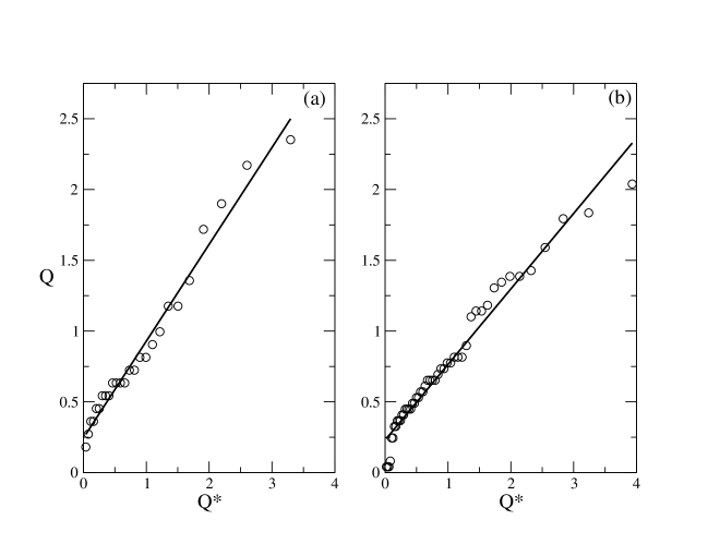
Figure 3: Quantile-quantileplot.Q∗:thestandardexponentialquantile.Q:quantilesforthewaterleveloftheHuangHeriver.Figure(a):quantile-quantileplotforthefirsthalfofthetimeseries.Figure(b):quantile-quantileplotforthesecondhalfofthetimeseries(afterthedropofthewaterlevel).