Synthesizing Datalog Programs Using Numerical Relaxation

Abstract

The problem of learning logical rules from examples arises in diverse fields, including program synthesis, logic programming, and machine learning. Existing approaches either involve solving computationally difficult combinatorial problems, or performing parameter estimation in complex statistical models.

In this paper, we present Difflog, a technique to extend the logic programming language Datalog to the continuous setting. By attaching real-valued weights to individual rules of a Datalog program, we naturally associate numerical values with individual conclusions of the program. Analogous to the strategy of numerical relaxation in optimization problems, we can now first determine the rule weights which cause the best agreement between the training labels and the induced values of output tuples, and subsequently recover the classical discrete-valued target program from the continuous optimum.

We evaluate Difflog on a suite of 34 benchmark problems from recent literature in knowledge discovery, formal verification, and database query-by-example, and demonstrate significant improvements in learning complex programs with recursive rules, invented predicates, and relations of arbitrary arity.

1 Introduction

As a result of its rich expressive power and efficient implementations, the logic programming language Datalog has witnessed applications in diverse domains such as bioinformatics Seo (2018), big-data analytics Shkapsky et al. (2016), robotics Poole (1995), networking Loo et al. (2006), and formal verification Bravenboer and Smaragdakis (2009). Users on the other hand are often unfamiliar with logic programming. The programming-by-example (PBE) paradigm aims to bridge this gap by providing an intuitive interface for non-expert users Gulwani (2011).

Typically, a PBE system is given a set of input tuples and sets of desirable and undesirable output tuples. The central computational problem is that of synthesizing a Datalog program, i.e., a set of logical inference rules which produces, from the input tuples, a set of conclusions which is compatible with the output tuples. Previous approaches to this problem focus on optimizing the combinatorial exploration of the search space. For example, Alps maintains a small set of syntactically most-general and most-specific candidate programs Si et al. (2018), Zaatar encodes the derivation of output tuples as a SAT formula for subsequent solving by a constraint solver Albarghouthi et al. (2017), and inductive logic programming (ILP) systems employ sophisticated pruning algorithms based on ideas such as inverse entailment Muggleton (1995). Given the computational complexity of the search problem, however, these systems are hindered by large or difficult problem instances. Furthermore, these systems have difficulty coping with minor user errors or noise in the training data.

In this paper, we take a fundamentally different approach to the problem of synthesizing Datalog programs. Inspired by the success of numerical methods in machine learning and other large scale optimization problems, and of the strategy of relaxation in solving combinatorial problems such as integer linear programming, we extend the classical discrete semantics of Datalog to a continuous setting named Difflog, where each rule is annotated with a real-valued weight, and the program computes a numerical value for each output tuple. This step can be viewed as an instantiation of the general $K$-relation framework for database provenance Green et al. (2007) with the Viterbi semiring being chosen as the underlying space $K$ of provenance tokens. We then formalize the program synthesis problem as that of selecting a subset of target rules from a large set of candidate rules, and thereby uniformly capture various methods of inducing syntactic bias, including syntax-guided synthesis (SyGuS) Alur et al. (2015), and template rules in meta-interpretive learning Muggleton et al. (2015).

The synthesis problem thus reduces to that of finding the values of the rule weights which result in the best agreement between the computed values of the output tuples and their specified values ($1$ for desirable and $0$ for undesirable tuples). The fundamental NP-hardness of the underlying decision problem manifests as a complex search surface, with local minima and saddle points. To overcome these challenges, we devise a hybrid optimization algorithm which combines Newton’s root-finding method with periodic invocations of a simulated annealing search. Finally, when the optimum value is reached, connections between the semantics of Difflog and Datalog enable the recovery of a classical discrete-valued Datalog program from the continuous-valued optimum produced by the optimization algorithm.

A particularly appealing aspect of relaxation-based synthesis is the randomness caused by the choice of the starting position and of subsequent Monte Carlo iterations. This manifests both as a variety of different solutions to the same problem, and as a variation in running times. Running many search instances in parallel therefore enables stochastic speedup of the synthesis process, and allows us to leverage compute clusters in a way that is fundamentally impossible with deterministic approaches. We have implemented Difflog and evaluate it on a suite of 34 benchmark programs from recent literature. We demonstrate significant improvements over the state-of-the-art, even while synthesizing complex programs with recursion, invented predicates, and relations of arbitrary arity.

Contributions.​​

Our work makes the following contributions:

1. A formulation of the Datalog synthesis problem as that of selecting a set of desired rules. This formalism generalizes syntax-guided query synthesis and meta-rule guided search.

2. A fundamentally new approach to solving rule selection by numerically minimizing the difference between the weighted set of candidate rules and the reference output.

3. An extension of Datalog which also associates output tuples with numerical weights, and which is a continuous refinement of the classical semantics.

4. Experiments showing state-of-the-art performance on a suite of diverse benchmark programs from recent literature.

2 Related Work

Weighted logical inference.​​

The idea of extending logical inference with weights has been studied by the community in statistical relational learning. Markov Logic Networks Richardson and Domingos (2006); Kok and Domingos (2005) view a first order formula as a template for generating a Markov random field, where the weight attached to the formula specifies the likelihood of its grounded clauses. ProbLog Raedt et al. (2007) extends Prolog with probabilistic rules and reduces the inference problem to weighted model counting. DeepProbLog Manhaeve et al. (2018) further extends ProbLog with neural predicates (e.g., input data can be images). These frameworks could potentially serve as the central inference component of our framework but we use the Viterbi semiring due to two critical factors: (a) the exact inference problem of these frameworks is #P-complete whereas inference in the Viterbi semiring is polynomial; and (b) automatic differentiation cannot easily be achieved without significantly re-engineering these frameworks.

Inductive logic programming (ILP).​​

The Datalog synthesis problem can be seen as an instance of the classic ILP problem. Metagol Muggleton et al. (2015) supports higher-order dyadic Datalog synthesis but the synthesized program can only consist of relations of arity two. Metagol is built on top of Prolog which limits its scalability, and also introduces issues with non-termination, especially when predicates have not already been partially ordered by the user. In contrast, ALPS Si et al. (2018) builds on top of Z3 fixed point engine and exhibits much better scalability. Recent works such as NeuralLP Yang et al. (2017) and $\partial$ILP Evans and Grefenstette (2018) reduce Datalog program synthesis to a differentiable end-to-end learning process by modeling relation joins as matrix multiplication, which also limits them to relations of arity two. NTP Rocktäschel and Riedel (2017) constructs a neural network as a learnable proof (or derivation) for each output tuple up to a predefined depth (e.g. $\leq 2$) with a few (e.g. $\leq 4$) templates, where the neural network could be exponentially large when either the depth or the number of templates grows. The predefined depth and a small number of templates could significantly limit the richness of learned programs. Our work seeks to synthesize Datalog programs consisting of relations of arbitrary arity and support rich features like recursion and predicate invention.

MCMC methods for program synthesis.​​

Markov chain Monte-Carlo (MCMC) methods have also been used for program synthesis. For example, in STOKE, Schkufza et al. (2016) apply the Metropolis-Hastings algorithm to synthesize efficient loop free programs. Similarly, Liang et al. (2010) show that program transformations can be efficiently learned from demonstrations by MCMC inference.

3 The Datalog Synthesis Problem

In this section, we concretely describe the Datalog synthesis problem, and establish some basic complexity results. We use the family tree shown in Figure 1 as a running example. In Section 3.1, we briefly describe how one may compute ${\small\mathrel{\textsf{samegen}}}(x,y)$ from ${\small\mathrel{\textsf{parent}}}(x,y)$ using a Datalog program. In Section 3.2, we formalize the query synthesis problem as that of rule selection.

(a)

Input tuples (EDB)
$\mathrel{\textsf{parent}}(\texttt{Will},\texttt{Noah})$
$\mathrel{\textsf{parent}}(\texttt{Ann},\texttt{Noah})$
$\mathrel{\textsf{parent}}(\texttt{Jim},\texttt{Emma})$
$\mathrel{\textsf{parent}}(\texttt{Ava},\texttt{Emma})$
$\mathrel{\textsf{parent}}(\texttt{Noah},\texttt{Liam})$
$\mathrel{\textsf{parent}}(\texttt{Emma},\texttt{Liam})$

(b)

Output tuples (IDB)
$\mathrel{\textsf{samegen}}(\texttt{Noah},\texttt{Emma})$
$\mathrel{\textsf{samegen}}(\texttt{Ann},\texttt{Will})$
$\mathrel{\textsf{samegen}}(\texttt{Jim},\texttt{Ann})$
$\cdots$

(c)

Figure 1: Example of a family tree (a), and its representation as a set of input tuples (b). An edge from $x$ to $y$ indicates that $x$ is a parent of $y$, and is represented symbolically as the tuple ${\small\mathrel{\textsf{parent}}}(x,y)$. The user wishes to realize the relation ${\small\mathrel{\textsf{samegen}}}(x,y)$, indicating the fact that $x$ and $y$ occur are from the same generation of the family (c).

3.1 Overview of Datalog

The set of tuples inhabiting relation ${\small\mathrel{\textsf{samegen}}}(x,y)$ can be computed using the following pair of inference rules, $r_{1}$ and $r_{2}$:

$$r_{1}\!\!:{\small\mathrel{\textsf{samegen}}}(x,y) \coloneq{\small\mathrel{\textsf{parent}}}(x,z),{\small\mathrel{\textsf{parent}}}(y,z).$$

$$r_{2}\!\!:{\small\mathrel{\textsf{samegen}}}(x,u) \coloneq{\small\mathrel{\textsf{parent}}}(x,y),{\small\mathrel{\textsf{parent}}}(u,v),{\small\mathrel{\textsf{samegen}}}(y,v).$$

Rule $r_{1}$ describes the fact that for all persons $x$, $y$, and $z$, if both $x$ and $y$ are parents of $z$, then $x$ and $y$ occur at the same level of the family tree. Informally, this rule forms the base of the inductive definition. Rule $r_{2}$ forms the inductive step of the definition, and provides that $x$ and $u$ occur in the same generation whenever they have children $y$ and $v$ who themselves occur in the same generation.

By convention, the relations which are explicitly provided as part of the input are called the EDB, $\mathcal{I}=\{{\small\mathrel{\textsf{parent}}}\}$, and those which need to be computed as the output of the program are called the IDB, $\mathcal{O}=\{{\small\mathrel{\textsf{samegen}}}\}$. To evaluate this program, one starts with the set of input tuples, and repeatedly applies rules $r_{1}$ and $r_{2}$ to derive new output tuples. Note that because of the appearance of the literal ${\small\mathrel{\textsf{samegen}}}(y,v)$ on the right side of rule $r_{2}$, discovering a single output tuple may recursively result in the further discovery of additional output tuples. The derivation process ends when no additional output tuples can be derived, i.e., when the set of conclusions reaches a fixpoint.

More generally, we assume a collection of relations, $\{P,Q,\dots\}$. Each relation $P$ has an arity $k\in\mathbb{N}$, and is a set of tuples, each of which is of the form $P(c_{1},c_{2},\dots,c_{k})$, for some constants $c_{1}$, $c_{2}$, …, $c_{k}$. The Datalog program is a collection of rules, where each rule $r$ is of the form:

$$P_{h}(\bm{u}_{h})\coloneq P_{1}(\bm{u}_{1}),P_{2}(\bm{u}_{2}),\dots,P_{k}(\bm{u}_{k}),$$

where $P_{h}$ is an output relation, and $\bm{u}_{h}$, $\bm{u}_{1}$, $\bm{u}_{2}$, …, $\bm{u}_{k}$ are vectors of variables of appropriate length. The variables $\bm{u}_{1}$, $\bm{u}_{2}$, …, $\bm{u}_{k}$, $\bm{u}_{h}$ appearing in the rule are implicitly universally quantified, and instantiating them with appropriate constants $\bm{v}_{1}$, $\bm{v}_{2}$, …, $\bm{v}_{k}$, $\bm{v}_{h}$ yields a grounded constraint $g$ of the form $P_{1}(\bm{v}_{1})\land P_{2}(\bm{v}_{2})\land\dots\land P_{k}(\bm{v}_{k})\implies P_{h}(\bm{v}_{h})$: “If all of the antecedent tuples $A_{g}=\{P_{1}(\bm{v}_{1}),P_{2}(\bm{v}_{2}),\dots,P_{k}(\bm{v}_{k})\}$ are derivable, then the conclusion $c_{g}=P_{h}(\bm{v}_{h})$ is also derivable.”

3.2 Synthesis as Rule Selection

The input-output examples, $I$, $O_{+}$, and $O_{-}$.​​

Instead of explicitly providing rules $r_{1}$ and $r_{2}$, the user provides an example instance of the EDB $I$, and labels a few tuples of the output relation as “desirable” or “undesirable” respectively:

$$O_{+}=\{{\small\mathrel{\textsf{samegen}}}({\small\texttt{Ann}},{\small\texttt{Jim}})\},\text{ and}$$

$$O_{-}=\{{\small\mathrel{\textsf{samegen}}}({\small\texttt{Ava}},{\small\texttt{Liam}}),{\small\mathrel{\textsf{samegen}}}({\small\texttt{Jim}},{\small\texttt{Emma}})\},$$

indicating that Ann and Jim are from the same generation, but Ava and Liam and Jim and Emma are not. Note that the user is free to label as many potential output tuples as they wish, and the provided labels $O_{+}\mathbin{\cup}O_{-}$ need not be exhaustive. The goal of the program synthesizer is to find a set of rules $R_{s}$ which produce all of the desired output tuples, i.e., $O_{+}\subseteq R_{s}(I)$, and none of the undesired tuples, i.e., $O_{-}\mathbin{\cap}R_{s}(I)=\emptyset$.

The set of candidate rules, $R$.​​

The user often possesses additional information about the problem instance and the concept being targeted. This information can be provided to the synthesizer through various forms of bias, which direct the search towards desired parts of the search space. A particularly common form in the recent literature on program synthesis is syntactic: for example, SyGuS requires a description of the space of potential solution programs as a context-free grammar Alur et al. (2015), and recent ILP systems such as Metagol Muggleton et al. (2015) require the user to provide a set of higher-order rule templates (“metarules”) and order constraints over predicates and variables that appear in clauses. In this paper, we assume that the user has provided a large set of candidate rules $R$ and that the target concept $R_{s}$ is a subset of these rules: $R_{s}\subseteq R$.

These candidate rules can express various patterns that could conceivably discharge the problem instance. For example, $R$ can include the candidate rule $r_{s}$, “${\small\mathrel{\textsf{samegen}}}(x,y)\coloneq{\small\mathrel{\textsf{samegen}}}(y,x)$”, which indicates that the output relation is symmetric, and the candidate rule $r_{t}$, “${\small\mathrel{\textsf{samegen}}}(x,z)\coloneq{\small\mathrel{\textsf{samegen}}}(x,y),{\small\mathrel{\textsf{samegen}}}(y,z)$”, which indicates that the relation is transitive. Note that the assumption of the candidate rule set $R$ uniformly subsumes many previous forms of syntactic bias, including those in SyGuS and Metagol.

Also note that $R$ can often be automatically populated: In our experiments in Section 6, we automatically generate $R$ using the approach introduced by Alps Si et al. (2018). We start with seed rules that follow a simple chain pattern (e.g., “$P_{1}(x_{1},x_{4})\coloneq P_{2}(x_{1},x_{2}),P_{3}(x_{2},x_{3}),P_{4}(x_{3},x_{4})$”), and repeatedly augment $R$ with simple edits to the variables, predicates, and literals of current candidate rules. The candidate rules thus generated exhibit complex patterns, including recursion, and contain literals of arbitrary arity. Furthermore, any conceivable Datalog rule can be produced with a sufficiently large augmentation distance.

Problem 1 (Rule Selection).

Let the following be given: (a) a set of input relations, $\mathcal{I}$ and output relations, $\mathcal{O}$, (b) the set of input tuples $I$, (c) a set of positive output tuples $O_{+}$, (d) a set of negative output tuples $O_{-}$, and (e) a set of candidate rules $R$ which map the input relations $\mathcal{I}$ to the output relations $\mathcal{O}$. Find a set of target rules $R_{s}\subseteq R$ such that:

$$O_{+}\subseteq R_{s}(I),\text{ and ~{}}O_{-}\mathbin{\cap}R_{s}(I)=\emptyset.$$

Finally, we note that the rule selection problem is NP-hard: this is because multiple rules in the target program $R_{s}$ may interact in non-compositional ways. The proof proceeds through a straightforward encoding of the satisfiability of a 3-CNF formula, and is provided in the Appendix.

Theorem 2.

Determining whether an instance of the rule selection problem, $(\mathcal{I},\mathcal{O},I,O_{+},O_{-},R)$, admits a solution is NP-hard.

4 A Smoothed Interpretation for Datalog

In this section, we describe the semantics of Difflog, and present an algorithm to evaluate and automatically differentiate this continuous-valued extension.

4.1 Relaxing Rule Selection

The idea motivating Difflog is to generalize the concept of rule selection: instead of a set of binary decisions, we associate each rule $r$ with a numerical weight $w_{r}\in[0,1]$. One possible way to visualize these weights is as the extent to which they are present in the current candidate program. The central challenge, which we will now address, is in specifying how the vector of rule weights $\bm{w}$ determine the numerical values $v_{t}^{R,I}(\bm{w})$ for the output tuples $t$ of the program. We use notation $v_{t}(\bm{w})$ when the set of rules $R$ and the set of input tuples $I$ are evident from context.

Every output tuple of a Datalog program is associated with a set of derivation trees, such as those shown in Figure 2. Let $r_{g}$ be the rule associated with each instantiated clause $g$ that appears in the derivation tree $\tau$. We define the value of $\tau$, $v_{\tau}(\bm{w})$, as the product of the weights of all clauses appearing in $\tau$, and the value of an output tuple $t$ as being the supremum of the values of all derivation trees of which it is the conclusion:

$$v_{\tau}(\bm{w})=\prod_{\text{clause }g\in\tau}w_{r_{g}},\text{ and}\ \ \ \ \ \$$ (1)

$$v_{t}(\bm{w})=\sup_{\tau\text{ with conclusion }t}v_{\tau}(\bm{w}),$$ (2)

with the convention that $\sup(\emptyset)=0$. For example, if $w_{r_{1}}=0.8$ and $w_{r_{2}}=0.6$, then the weight of the trees $\tau_{1}$ and $\tau_{2}$ from Figure 2 are respectively $v_{\tau_{1}}(\bm{w})=w_{r_{1}}=0.8$ and $v_{\tau_{2}}(\bm{w})=w_{r_{1}}w_{r_{2}}=0.48$.

(a)

(b)

Figure 2: Examples of derivation trees, $\tau_{1}$ (a) and $\tau_{2}$ (b) induced by various combinations of candidate rules, applied to the EDB of familial relationships from Figure 1. The input tuples are shaded in grey. We present two derivation trees for the conclusion ${\small\mathrel{\textsf{samegen}}}({\small\texttt{Will}},{\small\texttt{Ann}})$ using rules $r_{1}$ and $r_{2}$ in Section 3.1.

Since $0\leq w_{r}\leq 1$, it follows that $v_{\tau}(\bm{w})\leq 1$. Also note that a single output tuple may be the conclusion of infinitely many proof trees (see the derivation structure in Figure 3), leading to the deliberate choice of the supremum in Equation 2.

Figure 3: The rule $r_{s}$, “${\small\mathrel{\textsf{someone}}}(x,y)\coloneq{\small\mathrel{\textsf{samegen}}}(y,x)$”, induces cycles in the clauses obtained at fixpoint. When unrolled into derivation trees such as those in Figure 2, these cycles result in the production of infinitely many derivation trees for a single output tuple.

One way to consider Equations 1 and 2 is as replacing the traditional operations $(\land,\lor)$ and values $\{\text{true},\text{false}\}$ of the Boolean semiring with the corresponding operations $(\times,\max)$ and values $[0,1]$ of the Viterbi semiring. The study of various semiring interpretations of database query formalisms has a rich history motivated by the idea of data provenance. The following result follows from Prop. 5.7 in Green et al. (2007), and concretizes the idea that Difflog is a refinement of Datalog:

Theorem 3.

Let $R$ be a set of candidate rules, and $\bm{w}$ be an assignment of weights $w_{r}\in[0,1]$ to each of them, $r\in R$. Define $R_{s}=\{r\mid w_{r}\gneq 0\}$, and consider a potential output tuple $t$. Then, $v_{t}^{R,I}(\bm{w})\gneq 0$ iff $t\in R_{s}(I)$.

Furthermore, in the Appendix, we show that the output values $v_{t}(\bm{w})$ is well-behaved in its domain of definition:

Theorem 4.

The value of the output tuples, $v_{t}(\bm{w})$, varies monotonically with the rule weights $\bm{w}$, and is continuous in the region $0<w_{r}<1$.

We could conceivably have chosen a different semiring in our definitions in Equations 1 and 2. One alternative would be to choose a space of events, corresponding to the inclusion of individual rules, and choosing the union and intersection of events as the semiring operations. This choice would make the system coincide with ProbLog Raedt et al. (2007). However, the #P-completeness of inference in probabilistic logics would make the learning process computationally expensive. Other possibilities, such as the arithmetic semiring $(\mathbb{R},+,\times,0,1)$, would lead to unbounded values for output tuples in the presence of infinitely many derivation trees.

4.2 Evaluating and Automatically Differentiating Difflog Programs

Because the set of derivation trees for an individual tuple $t$ may be infinite, note that Equation 2 is merely definitional, and does not prescribe an algorithm to compute $v_{t}(\bm{w})$. Furthermore, numerical optimization requires the ability to automatically differentiate these values, i.e., to compute $\nabla_{\bm{w}}v_{t}$.

The key to automatic differentiation is tracking the provenance of each output tuple Green et al. (2007). Pick an output tuple $t$, and let $\tau$ be its derivation tree with greatest value. For the purposes of this paper, the provenance of $t$ is a map, $l_{t}=\{r\mapsto\#r\text{ in }\tau\mid r\in R\}$, which maps each rule $r$ to the number of times it appears in $\tau$. Given the provenance $l_{t}$ of a tuple, the derivative of $v_{t}(\bm{w})$ can be readily computed: $dv_{t}(\bm{w})/dw_{r}=l_{t}(r)v_{t}(\bm{w})/w_{r}$.

Algorithm 1 ${\small\textsc{Evaluate}}(R,\bm{w},I)$, where $R$ is a set of rules, $\bm{w}$ is an assignment of weight to each rule in $R$, and $I$ is a set of input tuples.

1. Initialize the set of tuples in each relation, $F_{P}\coloneqq\emptyset$, their valuations, $u(t)\coloneqq 0$, and their provenance $l(t)=\{r\mapsto\infty\mid r\in R\}$.

2. For each input relation $P$, update $F_{P}\coloneqq I_{P}$, and for each $t\in I_{P}$, update $u(t)\coloneqq 1$ and $l(t)=\{r\mapsto 0\mid r\in R\}$.

3. Until $(F,\bm{u})$ reach fixpoint,

   1. Compute the immediate consequence of each rule, $r$, “$P_{h}(\bm{u}_{h})\coloneq P_{1}(\bm{u}_{1}),P_{2}(\bm{u}_{2}),\dots,P_{k}(\bm{u}_{k})$”:

      $$F^{\prime}_{P_{h}}=\pi_{\bm{u}_{h}}(F_{P_{1}}(\bm{u}_{1})\bowtie F_{P_{2}}(\bm{u}_{2})\bowtie\cdots\bowtie F_{P_{k}}(\bm{u}_{k})).$$

      Furthermore, for each tuple $t\in F^{\prime}_{P_{h}}$, determine all sets of antecedent tuples, $A_{g}(t)=\{P_{1}(\bm{v}_{1}),P_{2}(\bm{v}_{2}),\dots,P_{k}(\bm{v}_{k})\}$, which result in its production.

   2. Update $F_{P_{h}}\coloneqq F_{P_{h}}\mathbin{\cup}F^{\prime}_{P_{h}}$.

   3. For each tuple $t\in F^{\prime}_{P_{h}}$ and each $A_{g}(t)$: (i) compute $u^{\prime}_{t}=w_{r}\prod_{i=1}^{k}u(P_{i}(\bm{v}_{i}))$, and (ii) if $u(t)<u^{\prime}_{t}$, update: $\displaystyle u(t)\coloneqq u^{\prime}_{t},\text{ and~{} }l(t)\coloneqq\{r\mapsto 1\}+\sum_{i=1}^{k}l(P_{i}(\bm{v}_{i})),$ where addition of provenance values corresponds to the element-wise sum.

4. Return $(F,\bm{u},\bm{l})$.

In Algorithm 1, we present an algorithm to compute the output values $v_{t}(\bm{w})$ and provenance $l_{t}$, given $R$, $\bm{w}$, and the input tuples $I$. The algorithm is essentially an instrumented version of the “naive” Datalog evaluator Abiteboul et al. (1995). We outline the proof of the following correctness and complexity claims in the Appendix.

Theorem 5.

Fix a set of input relations $\mathcal{I}$, output relations $\mathcal{O}$, and candidate rules $R$. Let ${\small\textsc{Evaluate}}(R,\bm{w},I)=(F,\bm{u},\bm{l})$. Then: (a) $F=R(I)$, and (b) $\bm{u}(t)=v_{t}(\bm{w})$. Furthermore, ${\small\textsc{Evaluate}}(R,\bm{w},I)$ returns in time $poly(|I|)$.

5 Formulating the Optimization Problem

We formulate the Difflog synthesis problem as finding the value of the rule weights $\bm{w}$ which minimizes the difference between the output values of tuples, $v_{t}(\bm{w})$, and their expected values, $1$ if $t\in O_{+}$, and $0$ if $t\in O_{-}$. Specifically, we seek to minimize the L2 loss,

$$L(\bm{w}) =\sum_{t\in O_{+}}(1-v_{t}(\bm{w}))^{2}+\sum_{t\in O_{-}}v_{t}(\bm{w})^{2}.$$ (3)

At the optimum point, Theorem 3 enables the recovery of a classical Datalog program from the optimum value $\bm{w}^{*}$.

Hybrid optimization procedure.

In program synthesis, the goal is often to ensure exact compatibility with the provided positive and negative examples. We therefore seek zeros of the loss function $L(\bm{w})$, and solve for this using Newton’s root-finding algorithm: $\bm{w}^{(i+1)}=\bm{w}^{(i)}-L(\bm{w})\nabla_{\bm{w}}L(\bm{w})/\|\nabla_{\bm{w}}L(\bm{w})\|^{2}$. To escape from local minima and points of slow convergence, we periodically intersperse iterations of the MCMC sampling, specifically simulated annealing. We describe the parameters of the optimization algorithm in the Appendix.

Separation-guided search termination.

After computing each subsequent $\bm{w}^{(i)}$, we examine the provenance values for each output tuple to determine whether the current position can directly lead to a solution to the rule selection problem. In particular, we compute the sets of desirable—$R_{+}=\{r\in l(t)\mid t\in O_{+}\}$—and undesirable rules—$R_{-}=\{r\in l(t)\mid t\in O_{-}\}$, and check whether $R_{+}\mathbin{\cap}R_{-}=\emptyset$. If these sets are separate, then we examine the candidate solution $R_{+}$, and return if it satisfies the output specification.

6 Empirical Evaluation

Our experiments address the following aspects of Difflog:

1. effectiveness at synthesizing Datalog programs and comparison to the state-of-the-art tool Alps Si et al. (2018), which already outperforms existing ILP tools Albarghouthi et al. (2017); Muggleton et al. (2015) and supports relations with arbitrary arity, sophisticated joins, and predicate invention;

2. the benefit of employing MCMC search compared to a purely gradient-based method; and

3. scaling with number of training labels and rule templates.

We evaluated Difflog on a suite of 34 benchmark problems Si et al. (2018). This collection draws benchmarks from three different application domains: (a) knowledge discovery, (b) program analysis, and (c) relational queries. The characteristics of the benchmarks are shown in Table 3 of the Appendix. These benchmarks involve up to 10 target rules, which could be recursive and involve relations with arity up to 6. The implementation of Difflog comprises 4K lines of Scala code. We use Newton’s root-finding method for continuous optimization and apply MCMC-based random sampling every 30 iterations. All experiments were conducted on Linux machines with Intel Xeon 3GHz processors and 64GB memory.

6.1 Effectiveness

We first evaluate the effectiveness of Difflog and compare it with Alps. The running time and solution of Difflog depends on the random choice of initial weights. Difflog exploits this characteristic by running multiple synthesis processes for each problem in parallel. The solution is returned once one of the parallel processes successfully synthesizes a correct Datalog program. We populated 32 processes in parallel and measured the running time until the first solution was found. The timeout is set to 1 hour for each problem.

Table 1: Characteristics of benchmarks and performance of Difflog compared to Alps. Rel shows the number of relations. Rule represents the number of expected (Exp) and candidate rules (Cnd). Tuple shows the number of input and output tuples. Iter and Smpl report the number of iterations and MCMC samplings. Time shows the running time of Difflog and Alps in seconds.

Benchmark	Rel	Rule		Tuple		Difflog			Alps
		Exp	Cnd	In	Out	Iter	Smpl	Time	Time
inflamation	7	2	134	640	49	1	0	1	2
abduce	4	3	80	12	20	1	0	$<$ 1	2
animals	13	4	336	50	64	1	0	1	40
ancestor	4	4	80	8	27	1	0	$<$ 1	14
buildWall	5	4	472	30	4	5	1	7	67
samegen	3	3	188	7	22	1	0	2	12
scc	3	3	384	9	68	6	1	28	60
polysite	6	3	552	97	27	17	1	27	84
downcast	9	4	1,267	89	175	5	1	30	1,646
rv-check	5	5	335	74	2	1,205	41	22	195
andersen	5	4	175	7	7	1	0	4	27
1-call-site	9	4	173	28	16	4	1	4	106
2-call-site	9	4	122	30	15	25	1	53	676
1-object	11	4	46	40	13	3	1	3	345
1-type	12	4	70	48	22	3	1	4	13
escape	10	6	140	13	19	2	1	1	5
modref	13	10	129	18	34	1	0	1	2,836
sql-10	3	2	734	10	2	7	1	11	41
sql-14	4	3	23	11	6	1	0	$<$ 1	54
sql-15	4	2	186	50	7	902	31	875	11

Table 1 shows the running of Difflog and Alps. We excluded 14 out of 34 benchmarks that both Difflog and Alps solve within a second (13 benchmarks) or run out of time (1 benchmark). Difflog outperforms Alps on 19 of the remaining 20 benchmarks. In particular, Difflog is orders of magnitude faster than Alps on most of the program analysis benchmarks. Meanwhile, the continuous optimization may not be efficient when the problem has many local minimas and the space is not convex. For example, sql-15 has a lot of sub-optimal solutions that generate not only all positive output tuples but also some negative ones.

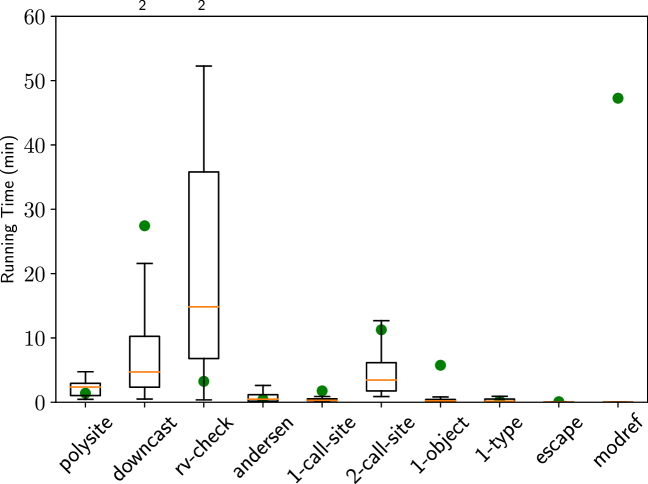
Figure 4: Distribution of Difflog’s running time from 32 parallel runs. The numbers on top represents the number of timeouts. Green circles represent the running time of Alps.

Figure 4 depicts the distribution of running time on the program analysis benchmarks. The results show that Difflog is always able to find solutions for all the benchmarks except for 2 timeouts for downcast and rv-check respectively. Also note that even the median running time of Difflog is smaller than the running time of Alps for 6 out of 10 benchmarks.

6.2 Impact of MCMC-based sampling

Table 2: Effectiveness of MCMC sampling in terms of the best running time (Time) and the number of timeouts (T/O).

Benchmark	Hybrid		Newton		MCMC
	Time	T/O	Time	T/O	Time	T/O
polysite	27	0	10	0	12	0
downcast	30	2	16	9	70	7
rv-check	22	2	N/A	32	N/A	32
andersen	4	0	3	10	4	9
1-call-site	4	0	8	1	N/A	32
2-call-site	53	0	27	17	42	9
1-object	3	0	3	17	N/A	32
1-type	4	0	3	18	N/A	32
escape	1	0	1	17	N/A	32
modref	1	0	1	4	N/A	32
Total		4		125		217

We next evaluate the impact of our MCMC-based sampling by comparing the performance of three variants of Difflog: a) a version that uses both Newton’s method and the MCMC-based technique (Hybrid), which is the same as in Section 6.1, b) a version that uses only Newton’s method (Newton), and c) a version that uses only the MCMC-based technique (MCMC). Table 2 shows the running time of the best run and the number of timeouts among 32 parallel runs for these three variants. The table shows that our hybrid approach strikes a good balance between exploitation and exploration. In many cases, Newton gets stuck in local minima; for example, it cannot find any solution for rv-check within one hour. MCMC cannot find any solution for 6 out of 10 benchmarks. Overall, Hybrid outperforms both Newton and MCMC by reporting 31$\times$ and 54$\times$ less number of timeouts, respectively.

6.3 Scalability

We next evaluate the scalability of Difflog, which is essentially affected by two factors: the number of templates and the size of training data. Our general observation is that increasing either of these does not significantly increase the effective running time (i.e., the best of 32 parallel runs).

Figure 5 shows how running time increases with the number of templates. As shown in Figure 5(a), the running time distribution for 2-call-site tends to have larger variance when the number of templates increases, but the best running time (out of 32 i.i.d samples) only increases modestly. The running time distribution for downcast, shown in Figure 5(b), has a similar trend except that smaller number of templates does not always lead to smaller variance or faster running time. For instance, the distribution in the setting with 180 templates has larger variance and median than distributions in the subsequent settings with larger number of templates. This indicates that the actual combination of templates also matters.

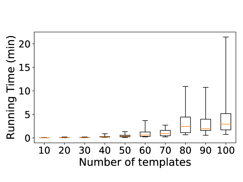
(a) 2-call-site

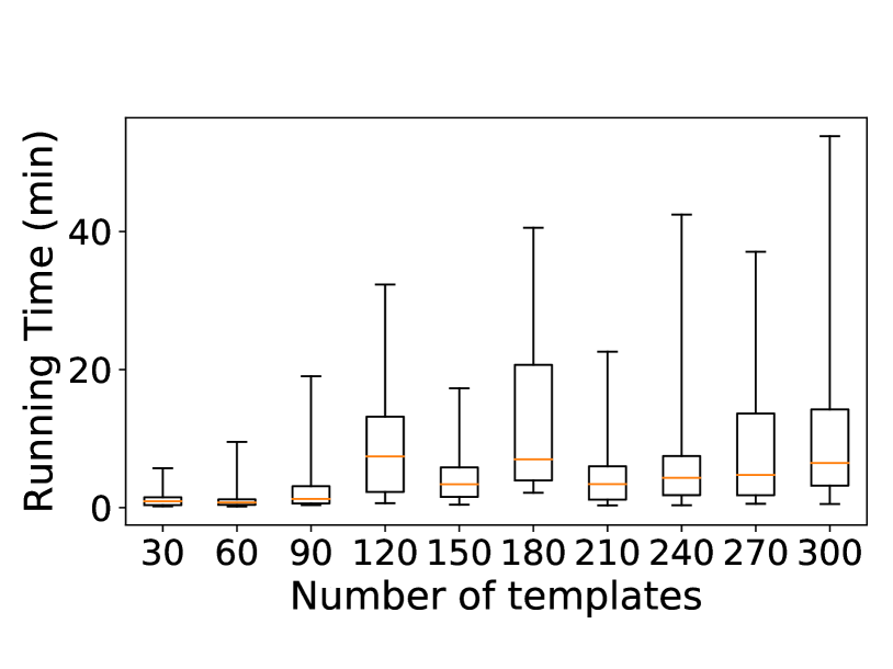
(b) downcast

Figure 5: Running time distributions for 2-call-site and downcast with different number of templates.

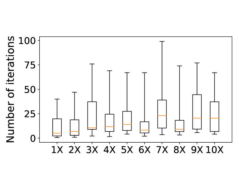
(a)

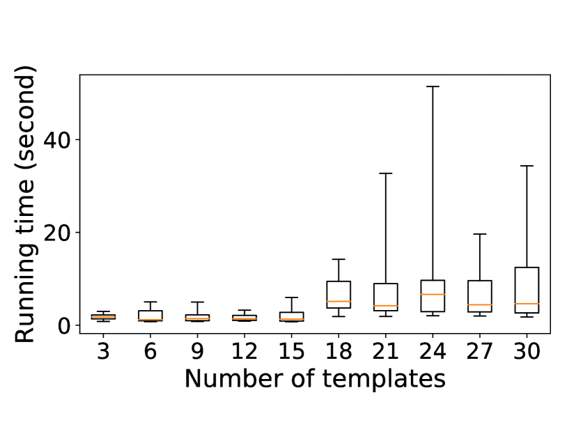
(b)

Figure 6: Performance of Difflog on andersen with different sizes of data: (a) the distribution of number of iterations, (b) the distribution of running time.

The size of training data is another important factor affecting the performance of Difflog. Figure 6(a) shows the distribution of the number of iterations for andersen with different sizes of training data. According to the results, the size of training data does not necessarily affect the number of iterations of Difflog. Meanwhile, Figure 6(b) shows that the end-to-end running time increases with more training data. This is mainly because more training data impose more cost on the Difflog evaluator. However, the statistics shows that the running time increases linearly with the size of data.

7 Conclusion

We presented a technique to synthesize Datalog programs by numerical optimization. The central idea was to formulate the problem as an instance of rule selection, and then relax classical Datalog to a refinement named Difflog. In a comprehensive set of experiments, we show that by learning a Difflog program and then recovering a classical Datalog program, we can achieve significant speedups over the state-of-the-art Datalog synthesis systems. In future, we plan to extend the approach to other synthesis problems such as SyGuS and to applications in differentiable programming.

Appendix A Proof of Theorems 2, 4 and 5

See 2

Proof.

Consider a 3-CNF formula $\varphi$ over a set $V$ of variables:

$$\varphi=(l_{11}\lor l_{12}\lor l_{13})\land(l_{21}\lor l_{22}\lor l_{23})\land\dots\land(l_{k1}\lor l_{k2}\lor l_{k3}),$$

be the given 3-CNF formula, where each literal $l_{ij}$ appearing in clause $c_{i}$ is either a variable, $v_{ij}\in V$, or its negation, $\lnot v_{ij}$. Assume that there are no trivial clauses in $\varphi$, which simultaneously contain both a variable and its negation. We will now encode its satisfiability as an instance of the rule selection problem.

1. For each variable $v\in V$, define the input relations:

   $${\small\mathrel{\textsf{pos}}}_{v} =\{(c)\mid v\in c\},\text{ and}$$ (4)

   $${\small\mathrel{\textsf{neg}}}_{v} =\{(c)\mid\lnot v\in c\},$$ (5)

   consisting of all one-place tuples ${\small\mathrel{\textsf{pos}}}_{v}(c)$ and ${\small\mathrel{\textsf{neg}}}_{v}(c)$ indicating whether the variable $v$ occurs positively or negatively in the clause $c$.

2. Also, for each variable $v$, define the input relation ${\small\mathrel{\textsf{var}}}_{v}$ which is inhabited by a single tuple ${\small\mathrel{\textsf{var}}}_{v}(v)$:

   $${\small\mathrel{\textsf{var}}}_{v} =\{(v)\}.$$ (6)

3. The idea is to set up the candidate rules so that subsets of chosen rules correspond to assignments of true / false values to the variables of $\varphi$. Let $C_{2}(c,v)$ be an output relation: we are setting up the problem so that if the tuple $C_{2}(c,v)$ is derivable in the synthesized solution, then there is a satisfying assignment of $\varphi$ where clause $c$ is satisfied due to the assignment to variable $v$.

4. For each variable $v$, create a pair of candidate rules $r_{v}$ and $r_{\lnot v}$ as follows:

   $$r_{v} =\text{``}C_{2}(c,v^{\prime})\coloneq{\small\mathrel{\textsf{pos}}}_{v}(c),{\small\mathrel{\textsf{var}}}_{v}(v^{\prime})\text{''},\text{ and}$$

   $$r_{\lnot v} =\text{``}C_{2}(c,v^{\prime})\coloneq{\small\mathrel{\textsf{neg}}}_{v}(c),{\small\mathrel{\textsf{var}}}_{v}(v^{\prime})\text{''}.$$

   Selecting the rule $r_{v}$ corresponds to assigning the value true to the corresponding variable $v$, and selecting the rule $r_{\lnot v}$ corresponds to assigning it the value false.

5. To prevent the simultaneous choice of rules $r_{v}$ and $r_{\lnot v}$, we set up the three-place input relation ${\small\mathrel{\textsf{conflict}}}(c,c^{\prime},v)$, which indicates that the reason for the simultaneous satisfaction of clauses $c$ and $c^{\prime}$ cannot be a contradictory variable $v$:

   $${\small\mathrel{\textsf{conflict}}} =\{(c,c^{\prime},v)\mid v\in c\text{ and }\lnot v\in c^{\prime}\}\mathbin{\cup}\{(a,a,a)\},$$ (7)

   where $a$ is some new constant not seen before. We will motivate its necessity while defining the canary output relation ${\small\mathrel{\textsf{error}}}$ next.

6. We detect the simultaneous selection of a pair of rules $r_{v}$ and $r_{\lnot v}$ using the rule $r_{e}$:

   $$r_{e}=\text{``}{\small\mathrel{\textsf{error}}}(c,c^{\prime},v)\coloneq C_{2}(c,v),C_{2}(c^{\prime},v),{\small\mathrel{\textsf{conflict}}}(c,c^{\prime},v)\text{''}$$

   Here ${\small\mathrel{\textsf{error}}}$ is a three-place output relation indicating the selection of an inconsistent assignment. We would like to force the synthesizer to choose the error-detecting rule $r_{e}$. The selection of the rule $r_{e}$, the presence of the input tuple ${\small\mathrel{\textsf{conflict}}}(a,a,a)$, and the selection of the rule $r_{a}$:

   $$r_{a}=\text{``}C_{2}(x,x)\coloneq{\small\mathrel{\textsf{conflict}}}(x,x,x)\text{''}$$

   is the only way to produce the output tuple ${\small\mathrel{\textsf{error}}}(a,a,a)$, which we will mark as desired.

7. The output tuple $C_{2}(c,v)$ indicates the satisfaction of the clause $c$ because of the assignment to variable $v$. We use the presence of such tuples to mark the clause $c$ itself as being satisfied: let $C_{1}(c)$ be a one-place output relation, and include the rule:

   $$r_{c}=\text{``}C_{1}(c)\coloneq C_{2}(c,v)\text{''}.$$

8. In summary, let the rule selection problem $P_{\varphi}=(\mathcal{I},\mathcal{O},I,O_{+},O_{-},R)$ be defined as follows:

   1. $\mathcal{I}=\{{\small\mathrel{\textsf{var}}}_{v},{\small\mathrel{\textsf{pos}}}_{v},{\small\mathrel{\textsf{neg}}}_{v}\mid v\in V\}\mathbin{\cup}\{{\small\mathrel{\textsf{conflict}}}\}$.

   2. $\mathcal{O}=\{C_{2},C_{1},{\small\mathrel{\textsf{error}}}\}$.

   3. Define the set of input tuples, $I$, using equations 4, 5, 6, and 7.

   4. $O_{+}=\{C_{1}(c)\mid\text{clause }c\in\varphi\}\mathbin{\cup}\{{\small\mathrel{\textsf{error}}}(a,a,a)\}$.

   5. $O_{-}=\{{\small\mathrel{\textsf{error}}}(c,c^{\prime},v)\mid\text{clauses }c,c^{\prime}\allowbreak\text{ and variable }v\allowbreak\text{ occurring in }\varphi\}$.

   6. $R=\{r_{v},r_{\lnot v}\mid v\in V\}\mathbin{\cup}\{r_{e},r_{a},r_{c}\}$.

Given a 3-CNF formula $\varphi$, the corresponding instance $P_{\varphi}$ of the rule selection problem can be constructed in polynomial time. Furthermore, it can be seen that, by construction, $P_{\varphi}$ admits a solution iff $\varphi$ is satisfiable. It follows that the rule selection problem is NP-hard. ∎

Next, we turn our attention to Theorem 4. The first part of the claim follows immediately from the definition in Equation 2. We therefore focus on the second part: Note that the proof of continuity does not immediately follow from Equation 2 because the supremum of an infinite set of continuous functions need not itself be continuous. It instead depends on the observation that there is a finite subset of dominating derivation trees whose values suffice to compute $v_{t}(\bm{w})$.

See 4

Proof.

Fix an assignment of rule weights $\bm{w}$. Next, focus on a specific output tuple $t$, and consider the set of all its derivation trees $\tau$. Let $\sigma_{\tau}$ be a pre-order traversal over its nodes. For example, for the tree $\tau_{1}$ in Figure 2(a), we obtain $\sigma_{\tau_{1}}={\small\mathrel{\textsf{samegen}}}({\small\texttt{Will}},{\small\texttt{Ann}}),\allowbreak r_{1}({\small\texttt{Will}},{\small\texttt{Ann}},{\small\texttt{Noah}}),\allowbreak{\small\mathrel{\textsf{parent}}}({\small\texttt{Will}},{\small\texttt{Noah}}),\allowbreak{\small\mathrel{\textsf{parent}}}({\small\texttt{Ann}},{\small\texttt{Noah}})$. It can be shown that the set of all pre-order traversals, $\sigma_{\tau}$, over all derivation trees $\tau$ forms a context-free grammar $L_{t}$.

We are interested in trees $\tau$ with high values $v_{\tau}(\bm{w})$, where the value of a tree depends only on the number of occurrences of each rule $r$. It therefore follows that the weight $v_{\tau}(\bm{w})$ is completely specified by the Parikh image, $\{r\mapsto\#r\text{ in }\tau\}$, which counts the number of occurrences of each symbol in each string of the language $L_{t}$. From Parikh’s lemma, we conclude that this forms a semilinear set. Let

$$p(L_{t})=\bigcup_{i=1}^{m}(\bm{c}_{i0}+\sum_{j=1}^{n}\bm{c}_{ij})$$

be the Parikh image of $L_{t}$, and for each $i\in\{1,2,\dots,m\}$, let $\tau_{i}$ be the derivation tree corresponding to the rule count $\bm{c}_{i0}$. It follows that:

$$v_{t}(\bm{w})=\sup_{\tau\text{ with conclusion }t}v_{\tau}(\bm{w})=\max_{i=1}^{m}v_{\tau_{i}}(\bm{w}).$$

We have reduced the supremum over an infinite set of continuous functions to the maximum of a finite set of continuous functions. It follows that $v_{t}(\bm{w})$ varies continuously with $\bm{w}$. ∎

Finally, we turn to the proof of Theorem 5.

See 5

Proof.

The first part of the following result follows from similar arguments as the correctness of the classical algorithm. We briefly describe the proof of the second claim. For each output tuple $t$, consider all of its derivation trees $\tau_{hi}$ with maximal value, and identify the tree $\tau_{t}$ with shortest height among these. All first-level sub-trees of $\tau_{t}$ must themselves possess the shortest-height-maximal-value property, so that their height is bounded by the number of output tuples. Since the $(F,\bm{u},\bm{l})$-loop in step 3 of Algorithm 1 has to hit a fixpoint within as many iterations, and since each iteration runs in polynomial time, the claim about running time follows. ∎

Appendix B Learning Details

We initialize $\bm{w}$ by uniformly sampling weights $w_{r}\in[0.25,0.75]$. We apply MCMC sampling after every 30 iterations of Newton’s root-finding method, and sample new weights as follows:

$$X\sim U(0,1)$$

$$w_{new}=\bigg{\{}\begin{tabular}[]{ll}$w_{old}\sqrt{2X}$&if $X<0.5$\\ $1-(1-w_{old})\sqrt{2(1-X)}$&otherwise.\end{tabular}$$

The temperature $T$ used in simulated annealing is as follows:

$$T=\frac{1.0}{C*log(5+\#iter)}$$

where C is initially 0.0001 and $\#iter$ is the number of iterations. We accept the newly proposed sample with probability

$$p_{acc}=\min(1,\pi_{new}/\pi_{curr}),$$

where $\pi_{curr}=\exp(-L_{2}(\bm{w}_{curr})/T)$ and $\pi_{new}=\exp(-L_{2}(\bm{w}_{new})/T)$.

Appendix C Benchmarks and Experimental Results

The characteristics of benchmarks are shown in Table 3. Figure 7 shows that the distribution of running time for the remaining benchmarks.

Table 3: Benchmarks characteristics. Rec and #Rel shows the programs that require recursive rules, and the number of relations. #Rules represents the number of expected (Exp) and candidate rules (Cand). #Tuples shows the number of input and output tuples.

	Benchmark	Rec	#Rel	#Rules		#Tuples
				Exp	Cand	In	Out
Knowelge Discovery	inflamation		7	2	134	640	49
	abduce		4	3	80	12	20
	animals		13	4	336	50	64
	ancestor	✓	4	4	80	8	27
	buildWall	✓	5	4	472	30	4
	samegen	✓	3	3	188	7	22
	path	✓	2	2	6	7	31
	scc	✓	3	3	384	9	68
Program Analysis	polysite		6	3	552	97	27
	downcast		9	4	1,267	89	175
	rv-check		5	5	335	74	2
	andersen	✓	5	4	175	7	7
	1-call-site	✓	9	4	173	28	16
	2-call-site	✓	9	4	122	30	15
	1-object	✓	11	4	46	40	13
	1-type	✓	12	4	70	42	15
	1-obj-type	✓	13	5	12	48	22
	escape	✓	10	6	140	13	19
	modref	✓	13	10	129	18	34
Relational Queries	sql-01		4	1	33	21	2
	sql-02		2	1	16	3	1
	sql-03		2	1	70	4	2
	sql-04		3	2	7	9	6
	sql-05		3	1	17	12	5
	sql-06		3	2	9	9	9
	sql-07		2	1	52	5	5
	sql-08		4	3	206	6	2
	sql-09		4	2	52	6	1
	sql-10		3	2	734	10	2
	sql-11		7	4	170	30	2
	sql-12		6	3	32	36	7
	sql-13		3	1	10	17	7
	sql-14		4	3	23	11	6
	sql-15		4	2	186	50	7

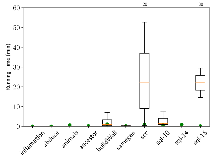
Figure 7: Distribution of Difflog’s running time from 32 parallel runs. The numbers on top represents the number of timeouts. Green circles represent the running time of Alps.

References

- Abiteboul et al. [1995] Serge Abiteboul, Richard Hull, and Victor Vianu. Foundations of Databases. Addison-Wesley, 1995.
- Albarghouthi et al. [2017] Aws Albarghouthi, Paraschos Koutris, Mayur Naik, and Calvin Smith. Constraint-based synthesis of datalog programs. In Proceedings of the 23rd International Conference on Principles and Practice of Constraint Programming, CP, pages 689–706, 2017.
- Alur et al. [2015] Rajeev Alur, Rastislav Bodík, Eric Dallal, Dana Fisman, Pranav Garg, Garvit Juniwal, Hadas Kress-Gazit, P. Madhusudan, Milo Martin, Mukund Raghothaman, Shambwaditya Saha, Sanjit Seshia, Rishabh Singh, Armando Solar-Lezama, Emina Torlak, and Abhishek Udupa. Syntax-guided synthesis. In Dependable Software Systems Engineering, pages 1–25. 2015.
- Bravenboer and Smaragdakis [2009] Martin Bravenboer and Yannis Smaragdakis. Strictly declarative specification of sophisticated points-to analyses. In Proceedings of the 24th Annual Conference on Object-Oriented Programming, Systems, Languages, and Applications, OOPSLA, pages 243–262, 2009.
- Evans and Grefenstette [2018] Richard Evans and Edward Grefenstette. Learning explanatory rules from noisy data (extended abstract). In Proceedings of the Twenty-Seventh International Joint Conference on Artificial Intelligence, IJCAI 2018, July 13-19, 2018, Stockholm, Sweden., pages 5598–5602, 2018.
- Green et al. [2007] Todd Green, Gregory Karvounarakis, and Val Tannen. Provenance semirings. In Proceedings of the 26th Symposium on Principles of Database Systems, PODS, pages 31–40, 2007.
- Gulwani [2011] Sumit Gulwani. Automating string processing in spreadsheets using input-output examples. In Proceedings of the 38th Symposium on Principles of Programming Languages, POPL, pages 317–330, 2011.
- Kok and Domingos [2005] Stanley Kok and Pedro M. Domingos. Learning the structure of markov logic networks. In Machine Learning, Proceedings of the Twenty-Second International Conference (ICML 2005), Bonn, Germany, August 7-11, 2005, pages 441–448, 2005.
- Liang et al. [2010] Percy Liang, Michael I. Jordan, and Dan Klein. Learning programs: A hierarchical bayesian approach. In Proceedings of the 27th International Conference on Machine Learning (ICML-10), June 21-24, 2010, Haifa, Israel, pages 639–646, 2010.
- Loo et al. [2006] Boon Thau Loo, Tyson Condie, Minos Garofalakis, David Gay, Joseph Hellerstein, Petros Maniatis, Raghu Ramakrishnan, Timothy Roscoe, and Ion Stoica. Declarative networking: Language, execution and optimization. In Proceedings of the 2006 International Conference on Management of Data, SIGMOD, pages 97–108, 2006.
- Manhaeve et al. [2018] Robin Manhaeve, Sebastijan Dumancic, Angelika Kimmig, Thomas Demeester, and Luc De Raedt. Deepproblog: Neural probabilistic logic programming. In Advances in Neural Information Processing Systems 31: Annual Conference on Neural Information Processing Systems 2018, NeurIPS 2018, 3-8 December 2018, Montréal, Canada., pages 3753–3763, 2018.
- Muggleton et al. [2015] Stephen H. Muggleton, Dianhuan Lin, and Alireza Tamaddoni-Nezhad. Meta-interpretive learning of higher-order dyadic Datalog: Predicate invention revisited. Machine Learning, 100(1):49–73, 2015.
- Muggleton [1995] Stephen Muggleton. Inverse entailment and Progol. New Generation Computing, 13(3&4):245–286, 1995.
- Poole [1995] David Poole. Logic programming for robot control. In Proceedings of the 14th International Joint Conference on Artificial Intelligence, IJCAI, pages 150–157, 1995.
- Raedt et al. [2007] Luc De Raedt, Angelika Kimmig, and Hannu Toivonen. Problog: A probabilistic prolog and its application in link discovery. In IJCAI 2007, Proceedings of the 20th International Joint Conference on Artificial Intelligence, Hyderabad, India, January 6-12, 2007, pages 2462–2467, 2007.
- Richardson and Domingos [2006] Matthew Richardson and Pedro M. Domingos. Markov logic networks. Machine Learning, 62(1-2):107–136, 2006.
- Rocktäschel and Riedel [2017] Tim Rocktäschel and Sebastian Riedel. End-to-end differentiable proving. In Advances in Neural Information Processing Systems 30: Annual Conference on Neural Information Processing Systems 2017, 4-9 December 2017, Long Beach, CA, USA, pages 3791–3803, 2017.
- Schkufza et al. [2016] Eric Schkufza, Rahul Sharma, and Alex Aiken. Stochastic program optimization. Commun. ACM, 59(2):114–122, 2016.
- Seo [2018] Jiwon Seo. Datalog extensions for bioinformatic data analysis. In 40th Annual International Conference of the IEEE Engineering in Medicine and Biology Society, EMBC, pages 1303–1306, 2018.
- Shkapsky et al. [2016] Alexander Shkapsky, Mohan Yang, Matteo Interlandi, Hsuan Chiu, Tyson Condie, and Carlo Zaniolo. Big data analytics with Datalog queries on Spark. In Proceedings of the 2016 International Conference on Management of Data, SIGMOD, pages 1135–1149, 2016.
- Si et al. [2018] Xujie Si, Woosuk Lee, Richard Zhang, Aws Albarghouthi, Paraschos Koutris, and Mayur Naik. Syntax-guided synthesis of Datalog programs. In Proceedings of the Joint Meeting on European Software Engineering Conference and Symposium on the Foundations of Software Engineering, FSE, pages 515–527, 2018.
- Yang et al. [2017] Fan Yang, Zhilin Yang, and William W. Cohen. Differentiable learning of logical rules for knowledge base reasoning. In Advances in Neural Information Processing Systems 30: Annual Conference on Neural Information Processing Systems 2017, 4-9 December 2017, Long Beach, CA, USA, pages 2316–2325, 2017.