Temporally Coherent Full 3D Mesh Human Pose Recovery from Monocular Video

Abstract

Advances in Deep Learning have recently made it possible to recover full 3D meshes of human poses from individual images. However, extension of this notion to videos for recovering temporally coherent poses still remains unexplored. A major challenge in this regard is the lack of appropriately annotated video data for learning the desired deep models. Existing human pose datasets only provide 2D or 3D skeleton joint annotations, whereas the datasets are also recorded in constrained environments. We first contribute a technique to synthesize monocular action videos with rich 3D annotations that are suitable for learning computational models for full mesh 3D human pose recovery. Compared to the existing methods which simply “texture-map” clothes onto the 3D human pose models, our approach incorporates Physics based realistic cloth deformations with the human body movements. The generated videos cover a large variety of human actions, poses, and visual appearances, whereas the annotations record accurate human pose dynamics and human body surface information. Our second major contribution is an end-to-end trainable Recurrent Neural Network for full pose mesh recovery from monocular video. Using the proposed video data and LSTM based recurrent structure, our network explicitly learns to model the temporal coherence in videos and imposes geometric consistency over the recovered meshes. We establish the effectiveness of the proposed model with quantitative and qualitative analysis using the proposed and benchmark datasets.

Keywords: Human Pose Recovery, 3D Human Reconstruction, Full Mesh Recovery, Data Synthesis.

1 Introduction

Recovering human poses from monocular (as opposed to multiview) images is an efficient approach since it does not require cumbersome calibration or high cost equipment. It has many applications in pose transfer, human movement analysis and action recognition. Until recently, the techniques used for human pose recovery aimed at predicting skeletal joint configurations from images [1, 2, 3, 4, 5]. However, recent findings [6, 7] ascertain that, using deep learning, it is possible to reconstruct full 3D human meshes from monocular images with the help of parameterized body and shape configurations [8]. Full 3D mesh recovery has clear advantages over the sparse skeleton recovery of human poses, as the former captures the inner pose dynamics as well as the outer 3D human bodies. These advantages multiply when, instead of individual images, human meshes can be recovered for full videos while incorporating the temporal dynamics of the body movement.

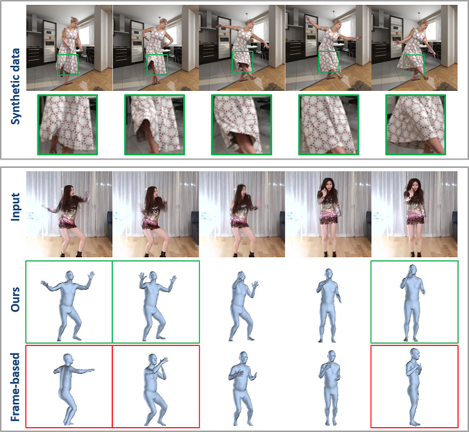
Figure 1: (Top) Illustration of realism in our data due to Physics based cloth movement. (Bottom) Compared to conventional frame-based 3D pose recovery [6], the proposed method better models the temporal variation and enforces geometric consistency of poses. The highlighted frames show frames where the difference between the two techniques is significant.

Video based full mesh recovery of human poses has further applications in precision modeling of human actions, virtual try-on, automatic animation, human-computer interaction and so on. However, progress in this research direction is currently hampered by the unavailability of appropriately annotated data for learning the desired computational models. Due to the constraints of sensor specifications, data modality and data sample size; existing datasets for human pose recovery, e.g. [9, 10, 2] are not particularly helpful in recovering full mesh poses from videos. On the other side, the requirement of panoptic studios [11] or full body scanners [12, 13] to annotate data for this task restrict researchers in generating specialized data for their specific problems in this area.

This work first addresses the problem of generating appropriately annotated training data to learn computational models that can recover full 3D meshes of human poses from monocular videos. To that end, we introduce a video generation technique that provides rich 3D annotations for realistic monocular videos. The generated videos are able to easily incorporate a wide variety of human actions and other visual variations related to e.g. cloth-body and cloth-gravity interactions, cloth textures, lighting conditions, camera viewpoints, and scene backgrounds. The annotations recorded for these videos include parameters of 3D human avatar (shape), 3D skeleton (pose) and its 2D image projection, and even the vertices of full human meshes (pose) in the videos. To accurately capture the movements of clothes and their interaction with human bodies, we employ a Physics engine that endows the generated videos with fine-grained realistic effects. To the best of our knowledge, this is the first of its kind ability of a data generation technique in the broader research direction of video/image based human action analysis. The videos/frames resulting from our technique are much more realistic as compared to those generated by the approaches that simulate clothes as textures on human models, see Fig. 1-top. The source code of our technique and the resulting data will be made public for the broader research community.

The second major contribution of this work is an end-to-end trainable Recurrent Neural Network that recovers full 3D human pose meshes from monocular video. The proposed network embeds a foundational building block that processes an individual video frame in a recurrent structure. We incorporate attention mechanism in the recurrent structure that provides contextual conditioning based on low-level visual features. The network precisely models the spatio-temporal dynamics of human movements in videos and imposes geometric consistency over the recovered mesh sequences by incorporating a body shape smoothness loss in the training process.

We analyze our technique using the proposed data and the benchmark Human3.6M [10] and UCF101 [14] datasets. Our experiments demonstrate that the proposed method is able to achieve very promising full mesh recovery for pose estimation from monocular video, e.g. Fig. 1-bottom. Due to the nascency of this research direction, this article also makes a minor contribution in introducing three new evaluation metrics to more appropriately analyze the mesh pose recovery from videos as compared to joint based pose recovery metrics used for individual video frames.

2 Related Work

Traditional techniques of human pose recovery usually apply pictorial structure models [15, 16, 17, 18, 19] to optimize body part configurations. However, due to the rapid advancements in deep learning, recovering articulated human poses using Convolutional Neural Network (CNN) models has become increasingly popular. For instance, Wei et al. [1] proposed Convolutional Pose Machines (CPM) to estimate 2D pose keypoints by learning a multi-stage CNN. The authors used a sequential convolutional structure to capitalize on the spatial context and iteratively updated the belief maps. In their method, the receptive field of neurons is carefully designed at each stage to allow the learning of complex and long-range correlations between the body parts. Similarly, Newell et al. [20] proposed a Stacked Hourglass method to process visual features across different scales. Their results are consolidated to better capture various spatial relationships associated with human body. Nevertheless, the CPM and Stacked Hourglass only work for static frame/images and do not account for any geometric consistency between different video frames.

To estimate 2D human poses in video, Pfister et al. [21] exploited the temporal context in video by combining information across multiple frames with optical flow. They used the resulting information to align heatmap predictions from the neighbouring frames. As a more recent attempt in modeling temporal information for human pose recovery, Luo et al. [5] re-modelled CPM as a Recurrent Neural Network to replace the multiple stages of CPM with sequential LSTM cells. The concept of using hand-crafted optical flow or recurrent structure to model temporal information in pose recovery task is beneficial. Nevertheless, both of these methods remain limited to recovering 2D keypoints only.

It is challenging to extend 2D keypoints recovery methods to recover 3D skeletons, as the latter demands sophisticated solutions. For example, Camillo [22] had to enforce additional constraints on the relative lengths of human limbs and the body joint kinematics to select valid limb configuration. Ramakrishna et al. [23] proposed an activity-independent technique to recover 3D joint configurations using 2D locations of anatomical landmarks. They also leveraged a large motion capture corpus as a proxy to infer the plausible 3D configurations. A few contributions in this direction have also formulated 3D skeleton recovery as a supervised learning problem. For instance, Pavlakos et al. [3] proposed a volumetric technique to estimate 3D human poses from a single image. Their volumetric representation converts the 3D coordinate regression problem to a more manageable prediction task in a discretized space. With this representation, they concatenated multiple fully convolutional network components to implement a iterative coarse-to-fine learning process.

Mehta et al. [24] enhanced CNN supervision with intermediate heat-maps, and used transfer learning from in-the-wild 2D pose data to improve the generalization to in-the-wild images for 3D pose recovery task. As a typical per-frame pose estimation technique, their method exhibits temporal jitters in video sequences. Another technique, VNect [2] formulates the 3D skeleton recovery problem as a CNN pose regression task that follows an optimization process, termed kinematic skeleton fitting. It is specifically designed to improve temporal stability of the recovered poses. Wang et al. [4] proposed a two-step technique for 3D pose estimation, named DRPose3D. In the first step, it uses a Pairwise Ranking CNN to extract depth rankings of human joints from images. In the second step, it uses this information to regress the 3D poses. This method depends on a 2D pose estimator for computing the initial joint heat maps. Consequently, it can not be treated as an end-to-end trainable technique.

Due to its attractive applications, full 3D mesh pose recovery from images is an emerging direction. Many recent methods adopt the parametric human model [8] in this regard. For instance, Alldieck et al. [25, 26, 27] inferred 3D shape of person with details including hair and cloth using parametric model. Yu et al. [28, 29] also used depth sensor to reconstruct 3D body shapes in cloth. They used cloth simulation for single view human performance capture. Kanazawa et al. [6] adopted the parametric human model for 3D mesh pose recovery and predicted its pose and shape parameters from monocular images in an end-to-end manner. Such a learning-based method requires training data with 3D annotations [30], a requirement fulfilled by very few datasets [10, 31]. The lack of training data has also driven research to exploit generative adversarial networks for 3D pose learning. Kanazawa et al. [6] used unpaired 3D annotations to create a factorized adversarial prior. Similarly, Yang et al. [7] learned a discriminator to enforce the 3D pose estimator to generate the plausible poses. However, a major limitation of such methods is that their complexity increases significantly when moving from frame to video modeling.

The challenges in manual annotation of large-scale data has also led researchers to synthesize annotated data. For instance, Lassner et al. [32] proposed a generative model to create people and manipulate their clothes. However, their method is frame-based which compromises the dynamic details of the clothes. Varol et al. [33] proposed SURREAL to synthesize human images for the tasks of body segmentation and depth estimation. Although SURREAL is able to generate RGB human images and 3D joints annotations it has multiple shortcomings. For instance, the variations of human actions are limited in SURREAL. Moreover, the images in the dataset remain unrealistic in terms of interaction between human models and their clothes. This happens because the data generation method simply wraps 2D cloth textures onto human models. Our literature survey reveals that end-to-end learning for 3D pose mesh recovery is a promising direction but remains largely unexplored due to the unavailability of large-scale data with rich 3D annotations. Moreover, due to single frame based benchmark datasets, existing methods are also limited to process individual frames. We address these issues by proposing a data generation method and a temporally coherent technique for full 3D mesh human pose recovery from videos.

3 Data Generation

As the first major contribution of this work, below we introduce our method of computationally generating human action videos with rich 3D annotations for training.

3.1 Human Pose and Shape Model

To represent human avatars, we use the Skinned Multi-Person Linear (SMPL) model [8] as parametric representation of human avatars in our data generation pipeline. SMPL provides a skinned vertex-based representation that can encode a wide variety of human body shapes in natural poses. The fact that SMPL model is created statistically using a large number of real humans also makes it suitable for the pose recovery task. An avatar in SMPL representation is given as a tuple $\mathcal{M}(\boldsymbol{\beta},\boldsymbol{\theta})$, where $\boldsymbol{\beta}$ and $\boldsymbol{\theta}$ respectively encode the body shape and pose. The body shape is parameterized by the first 10 coefficients of shape PCA space, hence $\boldsymbol{\beta}\in\mathbb{R}^{10}$. For $\boldsymbol{\theta}$, selected bones in human skeleton are represented in a hierarchical tree, where each bone/node is connected to its parent, and the whole skeleton is anchored to a root node. At each body joint $j$, an axis-angle rotation vector $\boldsymbol{\rho}_{j}\in\mathbb{R}^{3}$ controls the rotation of a child bone relative to its parent bone. The orientation of whole body is controlled by the root rotation vector $\boldsymbol{\rho}_{0}\in\mathbb{R}^{3}$. All of the above bone kinematics information is summarized by the pose parameter $\boldsymbol{\theta}\in\mathbb{R}^{3K}$, where $K=23$ for the $23$ body joints chosen by the SMPL representation.

In terms of SMPL representation, an avatar’s pose ${\bf P}_{i}\in\mathbb{R}^{3\times N}$ is a mapping of a tuple $\mathcal{M}_{i}(\boldsymbol{\beta}_{i},\boldsymbol{\theta}_{i})$ to $N=6890$ vertices describing the surface of an avatar. It is also possible to extract 2D keypoints and 3D skeletons using the technique of [8]. Our method uses the SMPL representation to record an avatar’s pose that is later rendered to a video frame using the graphics pipe-line discussed below.

3.2 Model Pose Variations

We exploit the CMU MoCap database (http://mocap.cs.cmu.edu) to bequeath the SMPL avatars with a large variety of natural poses and motions recorded using real humans. The CMU MoCap dataset covers more than $2500$ different action sequences that capture the dynamics of 3D skeleton joints. We use the MoSh technique [34] to map CMU joint locations to SMPL model parameter - resulting in human avatars. For a given CMU MoCap sequence, MoSh estimates the SMPL parameter $\boldsymbol{\theta}$ that best explains the body joint rotations corresponding to the CMU skeleton data. Multiple SMPL $\boldsymbol{\beta}$ parameters can then be chosen that animate the same action under different body shapes. We call the thus generated SMPL sequences as “MoShed” sequences.

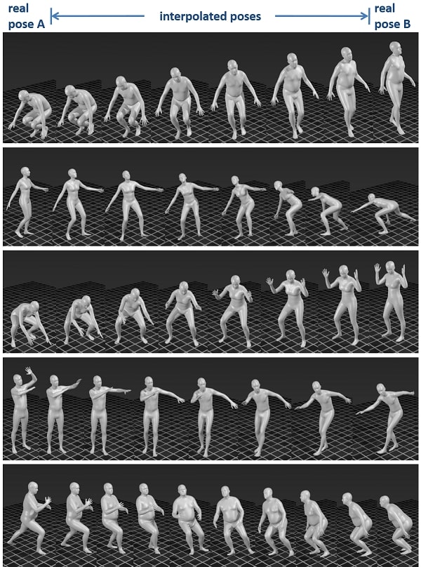
Figure 2: Illustration of pose interpolation: The first and last pose in each row are original poses, denoted as A and B. All the remaining poses in a row are generated by interpolating between their real pose A and B.

When using the MoShed CMU sequences, the pose variations are upper bounded by the total CMU pose types. To enhance the pose variations, we employ a pose interpolation technique to create new MoShed sequences that consist of novel poses. While interpolating between two poses, we choose widely contrasting poses as the starting and ending pose. See the real poses A and B in Fig. 2 as representative examples. This choice results in the interpolated poses that are significantly different from the available real pose sequences in the CMU dataset, improving the pose variety in our dataset.

The selection of contrasting real poses for the interpolation is made as follows. Consider two MoShed CMU MoCap sequences ${\bf X}=\{X_{i}\}_{i=1}^{m}$ and ${\bf Y}=\{Y_{j}\}_{j=1}^{n}$ that respectively contain $m$ and $n$ frames. Each frame in these sequences contains an independent human pose that is represented by SMPL pose parameter $\boldsymbol{\theta}$. We define the distance between a pair of human poses as $dist_{i,j}=||X_{i}(\boldsymbol{\theta})-Y_{j}(\boldsymbol{\theta})||_{2}$, and compute a distance matrix ${\bf D}\in\mathbb{R}^{m\times n}$ for all the pose pairs for action sequences ${\bf X}$ and ${\bf Y}$ using this distance. We select the two poses for interpolation by getting the frame indices $i,j=\text{argmax}({\bf D})$, and record $dist_{i,j}=\text{max}({\bf D})$. These pairs are used as the starting and ending frames for the creation of new pose sequence through interpolation.

As mentioned in Section 3.1, $\boldsymbol{\theta}\in\mathbb{R}^{3K}$ represents axis-angle rotation for each body joint relative to its parent bone. Compared to Quaternion rotation, Axis-angle rotation normalizes the rotation axis and multiplies it with the rotation magnitude. As $\boldsymbol{\theta}$ represents relative rotation and it works independently on each body joint, it is convenient to perform linear pose interpolation using the $\boldsymbol{\theta}$ parameters of the two poses. The number of interpolated frames is decided by the distance between the two frames. It can be observed in Fig. 2 that under this strategy, the transition between the two original poses remains smooth, whereas the interpolated poses appear as a person performing atypical actions. All the original and interpolated action sequences are used to render RGB action videos in our data generation scheme.

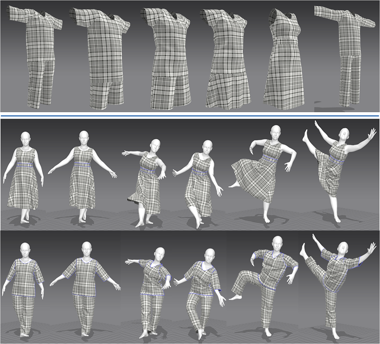
Figure 3: First row: Types of garments designed in this work to apply to SMPL models. Second and third row: Physics based application of garments to sequence of poses performing dance moves.

3.3 RGB Actions with Realistic Clothes

The avatars resulting from SMPL representation can only represent humans with minimal or tightly-fitted clothes. Consequently, previous attempts of using this representation to generate data in the broader domain of human actions, e.g. [35] extracted (unwrapped) texture maps from human scans, and fitted those onto the avatars. On one hand, the texture variations become limited under this strategy. On the other, this scheme does not correctly imitate clothes in the real-world. For instance, simple texture on an avatar does not behave in a ‘cloth-like’ manner, even for slightly loose clothes. Moreover, it does not cause any occlusion to the body shape, which is often there for the loose clothes. Not to mention, using only the texture also deprives the generated data of important temporal cues that cloth dynamics provide in the real-world actions.

We address this problem by modeling a number of garments for the SMPL avatars, and using those for data generation. In this work, the garment simulation is performed with a soft-body Physics engine. Such engines are used by fashion designing software, e.g. MarvelousDesigner7 (MD7) to achieve realistic effects. We adapt the engine from MD7 that supports cloth pattern cutting, sewing and its physical simulation. In the first row of Fig. 3, we illustrate different types of garment designed in this work. The second and third rows of the figure illustrate the results of applying two of these garments to a SMPL model under different poses of the avatar with the Physics engine based simulation. The shown six poses are sampled from a sequence (left to right) of a female avatar performing dance moves. Notice the realistic effects in terms of wrinkles, draping and the overall cloth movement in our data. We show a single texture design for all the avatars for better visualization. It is apparent that, applying static textures on avatars simply can not provide the fine details and the realistic interactions between cloth and human body that is provided by our technique. We also provide a qualitative comparison of the color frames constructed with our data generation technique with a popular existing method that uses texture-based clothing in Fig. 4.

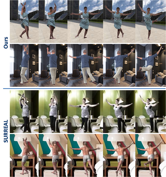
Figure 4: Comparison of an action sequence rendered by our method and SURREAL [35]. Our method enables fine cloth details and realistic cloth-body interactions, while SURREAL fits unwrapped textures onto the avatars, resulting in a less realistic “body-painting” effect. See the top of female affixed to legs in the bottom row.

We simulate cloth movements with the help of time-varying partial differential equations, which are solved as ordinary differential equations employing discritization [36]. In our case, a cloth is modelled as a set of particles $[m_{i},x_{i}]$ with interconnecting springs, where $m_{i}$ and $x_{i}$ are mass and geometric state vector of the $i$-th particle. The dynamics of the cloth is governed by the Newton‘s Equation:

$$m_{i}\ddot{x_{i}}=F_{int}+F_{ext},$$ (1)

where $F_{int}$ and $F_{ext}$ respectively denote the collective internal and external forces acting on the cloth, and $\ddot{x_{i}}$ is the second derivative of $x_{i}$ with respect to the time. Identifying the internal forces in cloth deformation is a hard problem. However, it can be reduced to the problem of differentiating the potential energy $E$ of the cloth particles spatially. This simplification leads to the following relationship:

$$-\frac{\partial E}{\partial x}=F_{int}.$$ (2)

The equation governing internal forces on a particle $x_{i}$ hence becomes,

$$m_{i}\ddot{x_{i}}=-[\frac{\partial E}{\partial x}]_{x=x_{i}}.$$ (3)

Putting the cloth particles into vectors, and accounting for the overall external forces, we can re-write our equation as:

$$M\ddot{x}=-\frac{\partial E}{\partial x}+F_{ext},$$ (4)

where M is a diagonal matrix formed with $m_{i}$, representing mass distribution of the cloth, and $F_{ext}$ models the extra external forces acting on the cloth as air-drag, contact and constraint forces, internal damping, etc. The overall external force on a cloth is also a function of $x$ as well as $\dot{x}$. Taking the time into account, the above equation can be written as

$$\ddot{x}(t)=M^{-1}(-\frac{\partial{E}}{\partial{x}}+F)(t).$$ (5)

Our Physics engine solves the above equation numerically [37] to get the time derivatives of the cloth particles. Using those with the particle locations results in realistic cloth deformations with its movements. The engine computes the Energy $E$ while accounting for the deformations of ‘stretch’, ‘shear’ and ‘bending’ for the realistic effects. Employing a Physics engine to simulate realistic cloth movements in 3D human videos is a unique contribution of this work. Our implementation and resulting data will be made public for the broader research community.

3.4 Scene Variations in Videos

We generate action videos that are rich in scene variations. We apply different backgrounds, cloth textures, illuminations, and viewpoints to render SMPL avatars to actual RGB frames. Below, we describe these variations and our method to incorporate them in more detail.

Background and cloth texture variations:  We use over 400 spherical images for the environmental backgrounds in our videos. These images are collected from online resources, such as Google Images. Our video generation pipeline additionally employs conventional 2D images for background during the rendering process. Towards that end, we exploit the Places365-Standard dataset [38] and use its test split to generate different backgrounds. We set the scales and rotations of the background scenes at random during the rendering process. To vary the cloth textures, we use the DTD [39] and Fabrics [40] datasets and randomly choose a texture for each video.

Lighting variations:  We setup four surface lights pointing towards the SMPL avatars and randomly change their strengths during rendering to simulate illumination variations encountered in the real-world scenes.

Viewpoint variations:  We render the moving SMPL avatar from four camera viewpoints setup in the East, West, South, and North of the avatar. To keep the avatars in the frame center, we set the cameras to track the Pelvis joint of the SMPL model. The camera sensor size and the focal length are set to 32mm and 180mm respectively, and the output resolution is fixed to 250 $\times$ 250. Since we use a telephoto camera, we carefully scale the background during the image rendering to better blend the rendered human models and their backgrounds. Different hyper-parameters of the setup discussed above are optimized empirically to achieve the best realistic visual appearances in the resulting videos.

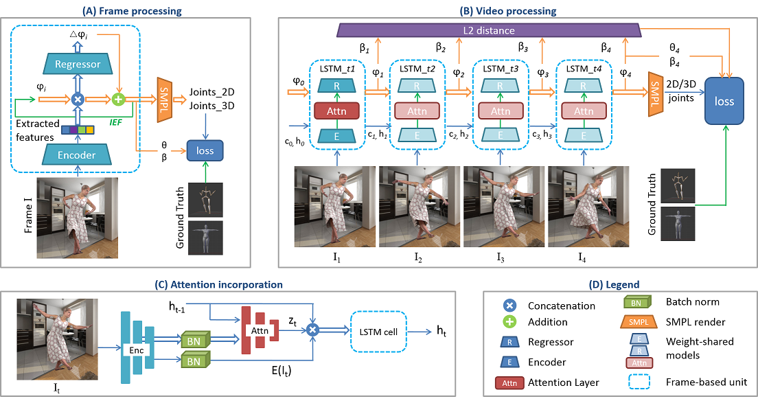
Figure 5: Approach schematics: (A) Basic building block to process individual frames. A frame ${\bf I}$ is encoded and a Regressor is trained using Iterative Error Feedback (IEF). Rich 3D annotations provide ground truth for SMPL parameters $\boldsymbol{\beta},\boldsymbol{\theta}$ and 2D, 3D skeletons. (B) The block is used in a recurrent setup with as many LSTM cells as the clip length that share Encoder and Regressor weights. An additional collective loss is defined over $\boldsymbol{\beta}_{t}$ for geometric consistency across the frames. The LSTM cells implicitly model temporal dynamics of a video. (C) Shows the attention mechanism that is incorporated to encode contextual information from low-level visual features to condition refreshing of the recurrent states. (D) Legend for the figure.

3.5 Synthesizing the Videos

Our data generation pipeline has three main steps to get from the MoShed CMU action sequences to realistic videos. In the first step, we import the SMPL avatar and its respective MoShed CMU sequences into Blender - an open source 3D rendering software (https://www.blender.org/) - and 3D render them. We achieve 3D avatar animation in this step with bodies that do not have clothes. In the second step, we apply clothes and perform Physics based simulation of the clothed avatars and record their mesh information. The physical properties of the clothes are preset to emulate realistic cloth-body and cloth-gravity interactions in this phase. In the third step, we again use the Blender with clothed meshes and synthesize videos by varying different scene attributes as discussed in §3.4.

Our cloth simulation requires human models in animation to start from a standard “T-shape” or “A-shape” pose, which are not guaranteed for many actions in CMU MoCap. To address this issue, we interpolate extra $N$ frames prior to the target MoCap action sequence, to ensure a smooth transition from a standard “T-shape”pose to the real poses of interest. In this work, we render videos for more than $5,000$ sequences using four different viewpoints. In total, we generate more than 3 million video frames in our dataset that can find applications in training deep models for various tasks, e.g. human action recognition, pose estimation.

4 Full Mesh Pose Recovery

The proposed data generation technique enables effective full mesh human pose sequence recovery directly from a video. To achieve this, we design a recovery mechanism for individual video frames and apply it in a recurrent structure for videos, as illustrated in Fig. 5.

4.1 Mesh Recovery from a Frame

Our data generation technique provides realistic video frames for which we also have rich 3D annotations. We use this data to learn a neural network model that can predict a 3D body mesh with accurate body shape and pose in individual frames. Concretely, this model predicts a vector $\boldsymbol{\varphi}=[\boldsymbol{\theta},\boldsymbol{\beta},{\bf R},{\bf t},s]$, where $\boldsymbol{\theta}$ and $\boldsymbol{\beta}$ are SMPL parameters (see §3.1), ${\bf R}\in\mathbb{R}^{3\times 3}$ describes the global rotation, ${\bf t}\in\mathbb{R}^{2}$ records the translation within the frame and $s\in\mathbb{R}$ is the scale of the 3D mesh. As shown in Fig. 5(A), there are two main components of the model, an ‘Encoder’ and a ‘Regressor’. We implement the Encoder as a CNN and the Regressor as an MLP. We defer the exact implementation details of these networks to §4.3 for continuity.

For an input video frame ${\bf I}$, the Encoder computes a feature vector $\mathcal{E}(I)\in\mathbb{R}^{D}$, which is regressed by the Regressor to estimate $\boldsymbol{\varphi}=\mathcal{R}(\mathcal{E}({\bf I}))$. To keep our model compact, we adopt Iterative Error Feedback (IEF) to train the Regressor. In IEF, the $i^{\text{th}}$ iteration computes $\boldsymbol{\varphi}_{i+1}=\boldsymbol{\varphi}_{i}+\Delta\boldsymbol{\varphi}_{i}$, where $\Delta\boldsymbol{\varphi}$ is the increment. This procedure is initialized with the $\boldsymbol{\varphi}$ resulting from the mean pose in our dataset. The predicted vector $\boldsymbol{\varphi}$ can be used to generate a 3D pose mesh ${\bf P}\in\mathbb{R}^{3\times N}$ under the SMPL representation. Moreover, this mesh can be regressed to achieve 3D skeleton [8] that we denote by ${}_{3D}\hat{{\bf J}}\in\mathbb{R}^{3\times Q}$, where $Q$ is the number of body joints. We further project the 3D joints to 2D key points as follows

$${}_{2D}\hat{{\bf J}}=s\boldsymbol{\Psi}({\bf R}~{}~{}_{3D}\hat{{\bf J}})+{\bf t},$$ (6)

where $\boldsymbol{\Psi}(.)$ is the orthographic projection operator. We use the 2D skeleton joints to define a ‘projection loss’

$$\mathcal{L}_{proj}=\sum\limits_{i}||\chi_{i}(_{2D}{\bf J}_{i}-_{2D}\hat{{\bf J}}_{i})||_{1},$$ (7)

where $\chi(.)$ is a masking operator that turns those joints to zero that are not visible in the ground truth 2D skeleton, and $||.||_{1}$ computes the $\ell_{1}$-norm. On similar lines, we also define a 3D joint loss as follows

$$\mathcal{L}_{3Djoint}=\sum\limits_{i}||_{3D}{\bf J}_{i}-_{3D}\hat{{\bf J}}_{i}||_{2}^{2}.$$ (8)

Moreover, we also define a SMPL parameter loss as

$$\mathcal{L}_{smpl}=\sum\limits_{i}||[\boldsymbol{\beta}_{i},\boldsymbol{\theta}_{i}]-[\hat{\boldsymbol{\beta}}_{i},\hat{\boldsymbol{\theta}}_{i}]||_{2}^{2}.$$ (9)

Finally, the overall loss for our network is defined as a combination of the above described losses, given as

$$\mathcal{L}=\mathcal{L}_{proj}+\delta(\mathcal{L}_{3Djoint}+\mathcal{L}_{smpl}).$$ (10)

In this formulation, the parameter $\delta$ is set to 1 when the ground truth 3D annotation is available and 0 otherwise. This parameter is useful when a training batch includes samples with only 2D keypoints annotations. Human pose recovery by Kanazawa et al. [6] can be related to our technique for frame based mesh recovery. However, our full mesh recovery method goes beyond individual frames to videos, as described below.

4.2 Mesh Recovery from a Video

Our data allows full mesh based supervised learning of deep models directly from videos, which was previously not possible. To recover meshes from videos, we treat our mechanism for frame processing (§ 4.1) as a basic building block and use it in a recurrent structure. We also incorporate attention layer in this recurrent model. The attention layer aims to encode low-level visual features of input images, and provide contextual conditions on the recurrent operations. The resulting technique explicitly models the temporal dynamics of action sequences and is able to enforce geometric consistency on the reconstructed poses across the frames. This makes the recovered 3D poses appear more natural and realistic, as illustrated in Fig. 1.

The proposed network for full mesh pose recovery is illustrated in Fig. 5 (B). We embed the frame-based building block in a recurrent structure by sharing the weights of the Encoder and Regressor. Given an input video clip $\{{\bf I}_{t}\}$, s.t. $t\in\{1,2,...,T\}$; where $T$ is the number of frames in the clip, the same Encoder is used to extract visual features from each frame. In addition to the feature vector $\mathcal{E}(I_{t})$, we probe the low-level feature map $\mathcal{E}(I_{t})_{low}\in\mathbb{R}^{L\times D}$, which can be represented as a set of annotation vectors $a_{t}=\{a_{t}^{1},...,a_{t}^{L}\}$, $a_{t}^{i}\in\mathbb{R}^{D}$. With an attention layer $f_{att}$ which is implemented as a multi-layer perceptron (MLP) [41], the context vector $\hat{z}_{t}$ of frame $\bf I_{t}$ is encoded with the annotation vectors $a_{t}$.

$$e_{t}^{i}=f_{att}(a_{t}^{i}),$$ (11)

$$\alpha_{t}^{i}=\frac{\mathrm{exp}(e_{t}^{i})}{\sum_{k=1}^{L}\mathrm{exp}(e_{t}^{k})}.$$ (12)

Here, $\alpha_{t}^{i}$ represents the weights of each annotation vector $a_{t}^{i}$ and $\sum_{i=1}^{L}\alpha_{t}^{i}=1$. Intuitively, it represents the importance of particular visual feature elements, and, therefore, indicates “where” and “how much” the network should pay attention to. With the calculated weights $\alpha_{t}^{i}$, we adopt a deterministic “soft” attention mechanism [42] to compute the context vector $\hat{z}_{t}$ as follows

$$\hat{z}_{t}=\sum_{i=1}^{L}{\alpha_{t}^{i}a_{t}^{i}}.$$ (13)

For the recurrent structure, we employ LSTM [43] for its gate and memory design that makes its training more effective. Following the implementation in [44], the overall behaviour of LSTM is represented mathematically by

$$c_{t}=f_{t}\odot c_{t-1}+i_{t}\odot g_{t},$$ (14)

$$h_{t}=o_{t}\odot\text{tanh}(c_{t}).$$ (15)

In the above equations, $i_{t},f_{t},c_{t},o_{t},h_{t}$ are the input, forget, memory, output and hidden state of the LSTM at time step $t$, and $\odot$ denotes the Hadamard product. Based on the above equations, we denote the LSTM cell function as $h_{t}=\Omega(i_{t})$ which controls the inflow and outflow of information through the LSTM at $t^{\text{th}}$ frame. The internal states of LSTM are controlled by the affine transformations with trainable parameters. The total time step of LSTM is set to $T$.

To incorporate the attention mechanism into the recurrent network, we make the context vector $\hat{z}_{t}$ conditioned on the previous hidden state of LSTM, i.e. $h_{t-1}$. Intuitively, as LSTM advances in a frame sequence, how the network pays its attention is conditioned on the information it has processed in the previous time steps. Hence, we can rewrite Eq. (11) as

$$e_{t}^{i}=f_{att}(a_{t}^{i},h_{t-1}).$$ (16)

Using the above configuration, the network computes the desired vector $\boldsymbol{\varphi}_{t}$ for the $t^{\text{th}}$ frame as

$$\boldsymbol{\varphi}_{t}=\mathcal{R}(\Omega(\mathcal{E}({\bf I}_{t})\otimes\hat{z}_{t}\otimes\boldsymbol{\varphi}_{t-1}));~{}t=1,2,...,T,$$ (17)

where $\otimes$ denotes vector concatenation. Note that, the input to an LSTM cell at each time step corresponds to the frame’s encoded feature augmented with the contextual information derived from low-level visual features, and the prediction from the last time step. At time 0, we assign the prediction $\boldsymbol{\varphi}_{0}$ as the mean value of SMPL parameters for our data. As for the cell state $c_{t}$ and the output state $h_{t}$, we initialize them as $(c_{0},h_{0})=\mathcal{I}(\mathcal{E}({\bf I}_{1}))$, where $\mathcal{I}(.)$ is implemented with an MLP with two hidden layers that maps an encoded feature vector to the initial states. This initialization strategy helps in faster training of the overall recurrent network.

To enforce geometric consistency along a predicted pose sequence, we propose an additional shape smoothness loss $\mathcal{L}_{shape}$, for the recurrent network as

$$\mathcal{L}_{shape}=\sum_{t=1}^{T-1}||\boldsymbol{\beta}_{t+1}-\boldsymbol{\beta}_{t}||_{2}^{2},$$ (18)

where $\boldsymbol{\beta}_{t}$ is obtained from the Regressor at the $t^{\text{th}}$ time stamp. In our recurrent structure, this loss inherently accounts for all the frames in a video clip. According to [1], intermediate supervision helps in mitigating the vanishing gradient problem in the recurrent networks, and also helps in better conditioning of the learning process. Hence, we eventually define our overall loss function as

$$\mathcal{L}=\sum_{t=1}^{T}\lambda((\mathcal{L}_{proj})_{t}+\delta\mathcal{(}L_{3D})_{t})+\mathcal{L}_{shape},$$ (19)

where $\mathcal{L}_{3D}\!\!=\!\!\mathcal{L}_{3Djoint}+\mathcal{L}_{smpl}$, and $\lambda$ is a hyper-parameter.

Table 1: 3D joint evaluation results on Human3.6M datasets: Evaluation metric PA-MPJPE, units mm. The proposed method is abbreviated as Mesh VIdeo PosE Recovery (MVIPER). Per action and mean error is reported for two evaluation protocols. See text for protocol description.

Protocol-1	Direc.	Discu.	Eat	Greet	Phone	Photo	Pose	Purchase	Sit	SitD.	Smoke	Wait	WalkD.	Walk	WalkT.	Mean
HMR [6]	52.3	54.7	54.3	57.1	60.9	70.4	51.6	49.9	65.7	76.0	58.6	52.5	60.2	45.2	53.6	57.5
HMR$\dagger$	51.2	52.4	53.8	56.9	59.9	65.0	50.4	49.2	66.3	73.1	59.2	52.6	60.0	46.6	53.9	56.7
MVIPER (ours)	48.1	48.8	49.6	55.3	53.8	63.4	49.4	48.0	58.5	67.4	54.4	52.2	59.3	47.3	54.3	54.0
Protocol-2	Direc.	Discu.	Eat	Greet	Phone	Photo	Pose	Purchase	Sit	SitD.	Smoke	Wait	WalkD.	Walk	WalkT.	Mean
SMPLify [45]	62.0	60.2	67.8	76.5	92.1	77.0	73.0	75.3	100.3	137.3	83.4	77.3	79.7	86.8	81.7	82.3
HMR [6]	53.2	56.8	50.4	62.4	54.0	72.9	49.4	51.4	57.8	73.7	54.4	50.0	62.6	47.1	55.0	56.7
HMR$\dagger$	52.1	53.9	51.4	61.1	54.4	66.1	49.6	48.7	58.3	69.9	54.6	50.0	60.6	49.3	55.5	55.7
MVIPER (ours)	48.0	46.0	46.0	57.1	48.6	61.3	47.7	46.8	54.1	67.1	48.9	50.1	59.1	47.8	56.1	52.3

4.3 Implementation Details

To implement the Encoder (E), we use the ResNet-50 model [46] pre-trained on ImageNet [47]. We consider the convolution activation prior to Softmax as an image feature, and the activation values of the layer “resnet-v2-50$/$block4” as the low-level feature map. We realize the Regressor (R) as a Multiple Layer Perceptron (MLP) with two fully-connected hidden layers, and an output layer that has the same dimension as vector $\boldsymbol{\varphi}$. Both E and R are shared by every time step for the LSTM, whereas we empirically set the width of the hidden unit for the LSTM to 2048, and use $T=4$. Our model for videos is trained in two main steps. First, we train a frame-based model and then use it in the second step for video based training. We copy the Encoder and Regressor weights for the recurrent model for initialization, and then train the model with stochastic gradient descent using Adam optimizer [48] in an end-to-end manner. We set the learning rate to $10^{-5}$, and batch size to 16.

To train a model, we also add samples from LSP, LSP-extended [49] MPII [50], MS COCO [9], Human3.6M [51] and MPIINF-3DHP [2] to our data, in addition to the proposed data. These datasets have been filtered to remove images that are too small or have less that 6 visible joints. The standard train/test split is used. Datasets such as LSP, COCO and MPII consist of independent frames, for which we replicate the individual frames to form training video clips.

5 Evaluation

5.1 Quantitative Evaluation

Metrics

Evaluation of a full 3D pose recovery method is not straightforward. It requires computing point-to-point errors between predicted and the ground truth ‘mesh’ points. For that, point-to-point mesh registration is required which is often not possible with the existing datasets. Consequently, recent works mostly resort to reporting Mean Per Joint Position Error (MPJPE) for 3D skeletons. For benchmarking, we also adopt MPJPE as one of our evaluation metrics. Nevertheless, since our data provides the possibility of point-to-point registration and mesh recovery directly from videos, we further introduce the following new metrics to more appropriately evaluate a model for video-based full mesh pose recovery: (a) Mean Per Vertex Position Error (MPVPE), (b) Mean Running Vertex Position Variation (MRVPV) and (c) Mean Running Shape Variation (MRSV).

We define the MPVPE as

$$\text{MPVPE}=\frac{1}{M}\sum_{j=1}^{M}\left(\sum_{i=1}^{N}||{\bf{\hat{v}}}_{i}-{\bf{v}}_{i}||_{2}\right),$$ (20)

where $M$ and $N$ respectively denote the frame length and the vertices in a mesh, and ${\bf v}_{i}$; and ${\bf\hat{v}}_{i}$ are the ground-truth and predicted vertex locations, respectively. This metric can be considered a mesh variant of MPJPE. To explicitly account for the temporal dimension of a video, we define MRVPV as

$$\text{MRVPV}=\frac{1}{M}\sum_{j=1}^{M-1}\left(\sum_{i=1}^{N}||{\bf\hat{v}}_{j+1,i}-{\bf\hat{v}}_{j,i}||_{p}\right),$$ (21)

where $||.||_{p}$ denotes the $\ell_{p}$-norm. We consider both $\ell_{1}$ and $\ell_{2}$ norms in this work, denoting the resulting variants by MRVPV₁ and MRVPV₂. We also define MRSV as

$$\text{MRSV}=\frac{1}{M}\sum_{i=1}^{M-1}\left(||\hat{\boldsymbol{\beta}}_{i+1}-\hat{\boldsymbol{\beta}}_{i}||_{p}\right),$$ (22)

denoting its $\ell_{1}$ and $\ell_{2}$ norm variants by MRSV₁ and MSRV₂, respectively. By definition, this metric gives an estimate of how well the shape of the computed avatar is maintained between consecutive video frames. A lower value ensures better geometric consistency in terms of the avatar shape.

Table 2: 3D Joint evaluation results on the proposed data.

Method	MPJPE	PA-MPJPE
SMPLify [45]	152.1	109.3
HMR [6]	133.2	81.3
HMR$\dagger$	125.6	77.6
MVIPER (ours)	93.2	60.5

3D Joints Evaluation

For 3D joint evaluation, we use the standard MPJPE metric. We also follow [45] to adjust the global misalignment for the reconstructed 3D joints by applying a similarity transform via the Procrustes Analysis (PA). The adjusted error is then reported as PA-MPJPE. We use both Human3.6M dataset and the proposed data for evaluation. Table 1 and Table 2 summarize our results, where our method is coined as Mesh VIdeo PosE Recovey (MVIPER). In the reported results, HMR$\dagger$ is our enhancement of HMR [6], which is achieved by fine tuning it on our dataset.

To achieve the results in Table 1, we follow the standard practice of using 5 subjects (ID: S1, S5, S6, S7, S8) for training and 2 subjects (ID: S9, S11) for testing. We employ two standard protocols. Protocol-1: uses samples from all four provided viewpoints for testing, and Protocol-2: uses only the frontal viewpoint samples. To evaluate MVIPER under frame based protocols, we replicate a frame multiple times to form a clip. In the Tables, our method is able to outperform the existing methods consistently. It is also notable that HMR$\dagger$ is able to perform better than HMR demonstrating the effectiveness of the proposed dataset for the task of 3D pose recovery in general. We note that this work focuses on recovering full 3D meshes, hence we include only those pose recovery methods in our comparisons that have this ability.

3D Mesh Evaluation

We evaluate the performance of our method for 3D pose mesh recovery from videos/images, and compare it with the existing SMPL-based methods that have the mesh recovery ability. Table 3 summarizes the results of our experiments using the evaluation metrics discussed above. As can be seen, the proposed method consistently outperforms the state-of-the-art 3D human pose mesh recovery methods. Again, the gain of HMR$\dagger$ over HMR demonstrates the effectiveness of the proposed dataset.

5.2 Ablation Study

The dataset proposed in this work enables learning 3D pose recovery models with full supervision in terms of 2D keypoints, 3D skeleton, and SMPL pose and shape parameters. Our model fully exploits these supervision labels for the pose recovery. In this section, we study the contribution of each of these supervision labels to the overall performance of our technique by re-training the MVIPER model with different loss combinations that are designed to capitalize on different supervision labels.

Table 3: 3D mesh evaluation on proposed dataset.

Method	MPVPE	MRSV1	MRSV2	MRVPV1	MRVPV2
SMPLify [45]	1426.9	0.85	0.41	257.9	4.64
HMR [6]	1056.5	0.82	0.36	194.0	4.31
HMR$\dagger$	923.7	0.76	0.32	191.2	4.25
MVIPER (ours)	692.7	0.51	0.29	178.7	4.02

The first column of Table 4 shows the loss combinations used for this ablation study. For each combination, we re-train the MVIPER model and report quantitative results on Human3.6M dataset under Protocol-1 and Protocol-2. Both MPJPE and the adjusted error PA-MPJPE are reported. The results clearly demonstrate the importance of direct 3D supervision for the pose recovery task. With 2D objective $\mathcal{L}_{proj}$, the model learning suffers from serious depth ambiguity. With 3D supervision, in both cases of $\mathcal{L}_{3Djoint}$ or $\mathcal{L}_{smpl}$, the accuracy improvement is remarkable. Considering rows 2 and 3 of the table, $\mathcal{L}_{proj}$+$\mathcal{L}_{3Djoint}$ achieves higher accuracy in MPJPE than $\mathcal{L}_{proj}$+$\mathcal{L}_{smpl}$, while both combinations have comparable performance with global alignment (PA-MPJPE). This is intuitive because both $\mathcal{L}_{3Djoint}$ and $\mathcal{L}_{smpl}$ reflect full 3D joints information, while $\mathcal{L}_{3Djoint}$ emphasizes more on the absolute joint locations, which benefits the 3D joints evaluation. The last row of Table 4 demonstrates that MVIPER achieves the best performance when we combine all the loss terms.

Table 4: Ablation study for training MVIPER with different loss combinations. For each row, MVIPER is re-trained with the designated losses and then evaluated on Human3.6M dataset. Definition of losses can be found in Section 4.1.

	Protocol-1		Protocol-2
Loss Combinations	MPJPE	PA-MPJPE	MPJPE	PA-MPJPE
$\mathcal{L}_{proj}$	139.0	72.6	117.3	67.2
$\mathcal{L}_{proj}$+$\mathcal{L}_{3Djoint}$	82.6	56.4	83.7	55.7
$\mathcal{L}_{proj}$+$\mathcal{L}_{smpl}$	110.7	58.2	105.3	57.6
$\mathcal{L}_{3Djoint}$+$\mathcal{L}_{smpl}$	83.8	58.0	88.9	58.3
$\mathcal{L}_{proj}$+$\mathcal{L}_{3Djoint}$+$\mathcal{L}_{smpl}$	82.2	54.0	81.5	52.3

5.3 Qualitative Evaluation

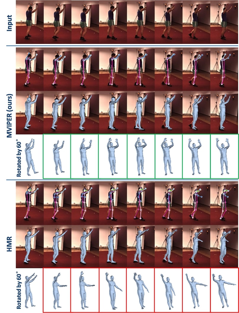
Figure 6: Qualitative comparison for HMR and our approach on Human3.6M. For each method, the recovered mesh and its 60^∘ rotation are displayed. The rotated meshes are shown for better visualization.

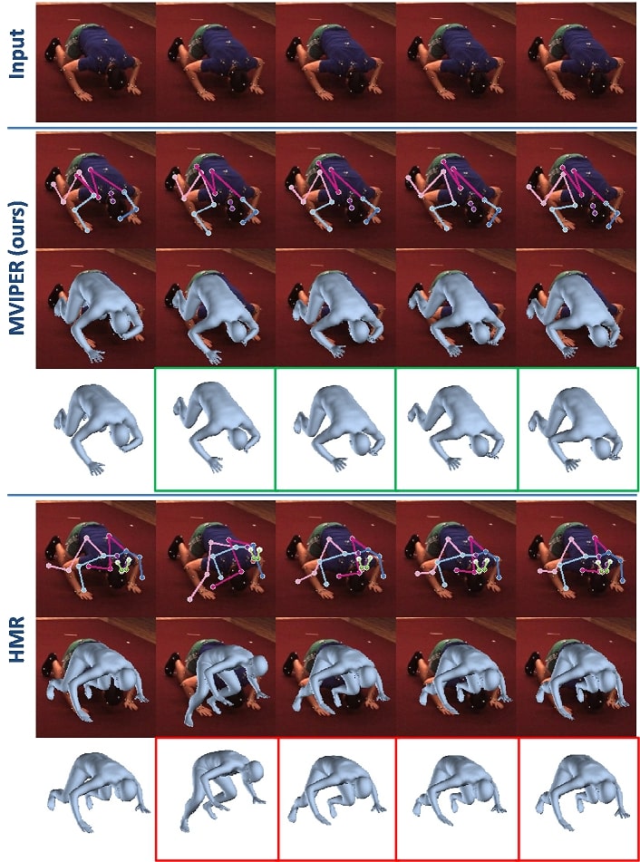
Figure 7: Qualitative comparison for HMR and our approach on Human3.6M. Our approach recovers more accurate and coherent pose sequence.

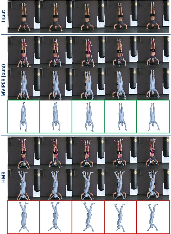
Figure 8: Qualitative comparison. Challenging “handstand” poses are accurately recovered by our method because it benefits from a large amount of pose variations that are present in the proposed dataset.

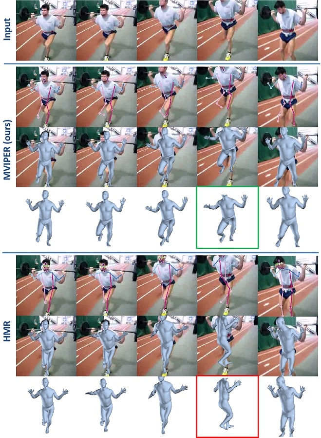
Figure 9: Qualitative comparison. HMR suffers from a sudden body orientation error, as it does not consider the temporal context from neighbouring frames.

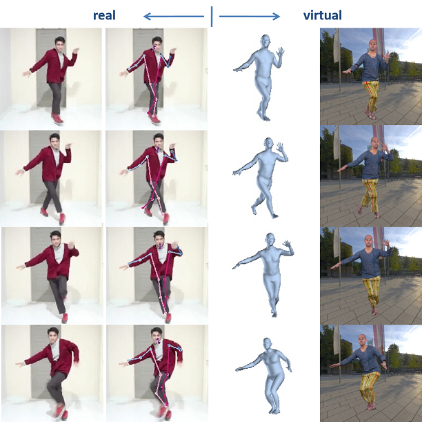
Figure 10: Example of motion transfer performed using the proposed MVIPER. Motions are transferred from real to virtual world with new cloth and background in the virtual world.

Representative examples for qualitative performance comparison between our method and the competing frame-based technique, i.e. HMR is shown in Fig. 6 and Fig. 7. The examples are selected at random from Human3.6M dataset. Note that, Human3.6M dataset does not provide ground truth for 3D meshes, hence we can only show the qualitative results. In Fig. 6, when the performer’s left arm is occluded by body, HMR loses its spatial cues and fails to reconstruct it appropriately, while our approach is able to construct the left arm properly by accounting for the temporal cues. The 60^∘ rotation of mesh is provided for better visualization. Similarly, for the complex motions, as illustrated in Fig. 7, HMR also fails to recover accurate and consistent poses. On the other hand, the proposed method performs a much more accurate pose recovery.

In addition to Human3.6M, we further conducted qualitative analysis on UCF101 [14] - an “in-the-wild” action dataset unseen by our method and the benchmark HMR method during training. From the UCF101 dataset, we selected action sequences in which body motions represent the major contents of video frames. We show representative qualitative results on this dataset in Fig. 8. and Fig. 9. For each sequence evaluated by MVIPER and HMR, we highlight the frames which show significant quality difference. Our method demonstrates consistent advantage over frame-based HMR. In Fig. 8, HMR fails to recover the uncommon “handstand” poses, while our method recovers it properly. We attribute this difference to our synthetic training data which includes more pose variations, and hence improves the performance of the resulting model. As our method models temporal variations and imposes geometric consistency, it is able to generate smooth transition for recovered pose sequences. On the other hand, frame-based methods like HMR suffer from temporal jitters and sudden orientation error as visible in Fig. 9.

5.4 Video-based Motion Transfer

This is the first work to explore video-based full mesh pose recovery. This problem can find many interesting applications in e.g. animations. As a possible application of our approach we explore video-based motion transfer. In this application, we input a real-world video of a human performing an action and transfer that motion to an avatar in virtual world. The proposed MVIPER uses the input video to compute 3D meshes for each frame, which are subsequently rendered with different cloths and backgrounds to create virtual actions. The whole process transfers a real-life human motion to a virtual world avatar. We illustrate a representative example from this experiment in Fig. 10. As can be seen, the proposed technique is able to transfer the motion with good fidelity due to accurate human mesh recovery.

6 Conclusion

We proposed a data generation technique and an end-to-end trainable RNN to recover full 3D meshes of human poses directly from monocular videos. Our data generation method exploits Computer Graphics to generate realistic action videos with a large amount of scene variations in backgrounds, cloth textures, illuminations and viewpoints. To further enhance action and pose variations in the generated data, pose interpolation is employed to create novel pose sequences between largely varied pose pairs. Moreover, we embed a Physics engine in data generation to produces vivid cloth deformations and cloth-body interactions. This is the first successful application of a Physics engine in contemporary human data synthesis technique for learning deep models. By using the proposed action video dataset and a parameterized human model, we also developed a neural network for video-based full mesh pose recovery. Our network embeds a basic building block in a recurrent structure and explicitly encodes temporal variations of input video frames, and imposes geometric consistency over the recovered meshes across the video frames. We evaluated the proposed method on our dataset and Human3.6M, using conventional per-joint error metrics, as well as more advanced per-vertex error metrics introduced in this work. Qualitative comparison is provided on Human3.6M and UCF101 action datasets. Both quantitative and qualitative results demonstrate that our method achieves very promising results for full mesh pose recovery from videos.

References

- [1] S.-E. Wei, V. Ramakrishna, T. Kanade, and Y. Sheikh, “Convolutional pose machines,” in CVPR, 2016, pp. 4724–4732.
- [2] D. Mehta, S. Sridhar, O. Sotnychenko, H. Rhodin, M. Shafiei, H.-P. Seidel, W. Xu, D. Casas, and C. Theobalt, “Vnect: Real-time 3d human pose estimation with a single rgb camera,” ACM Transactions on Graphics, vol. 36, no. 4, p. 44, 2017.
- [3] G. Pavlakos, X. Zhou, K. G. Derpanis, and K. Daniilidis, “Coarse-to-fine volumetric prediction for single-image 3d human pose,” in CVPR. IEEE, 2017, pp. 1263–1272.
- [4] M. Wang, X. Chen, W. Liu, C. Qian, L. Lin, and L. Ma, “Drpose3d: Depth ranking in 3d human pose estimation,” IJCAI, 2018.
- [5] Y. Luo, J. Ren, Z. Wang, W. Sun, J. Pan, J. Liu, J. Pang, and L. Lin, “Lstm pose machines,” in CVPR. IEEE, 2018, pp. 5207–5215.
- [6] A. Kanazawa, M. J. Black, D. W. Jacobs, and J. Malik, “End-to-end recovery of human shape and pose,” in CVPR, 2018, pp. 7122–7131.
- [7] W. Yang, W. Ouyang, X. Wang, J. Ren, H. Li, and X. Wang, “3d human pose estimation in the wild by adversarial learning,” in CVPR, vol. 1, 2018.
- [8] M. Loper, N. Mahmood, J. Romero, G. Pons-Moll, and M. J. Black, “Smpl: A skinned multi-person linear model,” ACM Transactions on Graphics, vol. 34, no. 6, p. 248, 2015.
- [9] T.-Y. Lin, M. Maire, S. Belongie, J. Hays, P. Perona, D. Ramanan, P. Dollár, and C. L. Zitnick, “Microsoft coco: Common objects in context,” in ECCV. Springer, 2014, pp. 740–755.
- [10] C. Ionescu, D. Papava, V. Olaru, and C. Sminchisescu, “Human3.6m: Large scale datasets and predictive methods for 3d human sensing in natural environments,” PAMI, vol. 36, no. 7, pp. 1325–1339, jul 2014.
- [11] H. Joo, H. Liu, L. Tan, L. Gui, B. Nabbe, I. Matthews, T. Kanade, S. Nobuhara, and Y. Sheikh, “Panoptic studio: A massively multiview system for social motion capture,” in Proceedings of the IEEE International Conference on Computer Vision, 2015, pp. 3334–3342.
- [12] G. Pons-Moll, S. Pujades, S. Hu, and M. J. Black, “Clothcap: Seamless 4d clothing capture and retargeting,” ACM Transactions on Graphics (TOG), vol. 36, no. 4, p. 73, 2017.
- [13] N. Mahmood, N. Ghorbani, N. F. Troje, G. Pons-Moll, and M. J. Black, “Amass: Archive of motion capture as surface shapes,” arXiv preprint arXiv:1904.03278, 2019.
- [14] K. Soomro, A. R. Zamir, and M. Shah, “Ucf101: A dataset of 101 human actions classes from videos in the wild,” arXiv preprint arXiv:1212.0402, 2012.
- [15] M. Andriluka, S. Roth, and B. Schiele, “Pictorial structures revisited: People detection and articulated pose estimation,” in CVPR. IEEE, 2009, pp. 1014–1021.
- [16] P. F. Felzenszwalb and D. P. Huttenlocher, “Pictorial structures for object recognition,” International journal of computer vision, vol. 61, no. 1, pp. 55–79, 2005.
- [17] B. Sapp, D. Weiss, and B. Taskar, “Parsing human motion with stretchable models,” in CVPR 2011. IEEE, 2011, pp. 1281–1288.
- [18] Y. Yang and D. Ramanan, “Articulated human detection with flexible mixtures of parts,” IEEE transactions on pattern analysis and machine intelligence, vol. 35, no. 12, pp. 2878–2890, 2013.
- [19] M. Andriluka, S. Roth, and B. Schiele, “Monocular 3d pose estimation and tracking by detection,” in 2010 IEEE Computer Society Conference on Computer Vision and Pattern Recognition. IEEE, 2010, pp. 623–630.
- [20] A. Newell, K. Yang, and J. Deng, “Stacked hourglass networks for human pose estimation,” in European Conference on Computer Vision. Springer, 2016, pp. 483–499.
- [21] T. Pfister, J. Charles, and A. Zisserman, “Flowing convnets for human pose estimation in videos,” in Proceedings of the IEEE International Conference on Computer Vision, 2015, pp. 1913–1921.
- [22] C. J. Taylor, “Reconstruction of articulated objects from point correspondences in a single uncalibrated image,” CVIU, vol. 80, no. 3, pp. 349–363, 2000.
- [23] V. Ramakrishna, T. Kanade, and Y. Sheikh, “Reconstructing 3d human pose from 2d image landmarks,” in ECCV. Springer, 2012, pp. 573–586.
- [24] D. Mehta, H. Rhodin, D. Casas, P. Fua, O. Sotnychenko, W. Xu, and C. Theobalt, “Monocular 3d human pose estimation in the wild using improved cnn supervision,” in 3D Vision (3DV). IEEE, 2017, pp. 506–516.
- [25] T. Alldieck, M. Magnor, W. Xu, C. Theobalt, and G. Pons-Moll, “Video based reconstruction of 3d people models,” in Proceedings of the IEEE Conference on Computer Vision and Pattern Recognition, 2018, pp. 8387–8397.
- [26] ——, “Detailed human avatars from monocular video,” in 2018 International Conference on 3D Vision (3DV). IEEE, 2018, pp. 98–109.
- [27] T. Alldieck, M. Magnor, B. L. Bhatnagar, C. Theobalt, and G. Pons-Moll, “Learning to reconstruct people in clothing from a single rgb camera,” arXiv preprint arXiv:1903.05885, 2019.
- [28] T. Yu, Z. Zheng, K. Guo, J. Zhao, Q. Dai, H. Li, G. Pons-Moll, and Y. Liu, “Doublefusion: Real-time capture of human performances with inner body shapes from a single depth sensor,” in Proceedings of the IEEE Conference on Computer Vision and Pattern Recognition, 2018, pp. 7287–7296.
- [29] T. Yu, Z. Zheng, Y. Zhong, J. Zhao, Q. Dai, G. Pons-Moll, and Y. Liu, “Simulcap: Single-view human performance capture with cloth simulation,” arXiv preprint arXiv:1903.06323, 2019.
- [30] M. Omran, C. Lassner, G. Pons-Moll, P. Gehler, and B. Schiele, “Neural body fitting: Unifying deep learning and model based human pose and shape estimation,” in 2018 International Conference on 3D Vision (3DV). IEEE, 2018, pp. 484–494.
- [31] L. Sigal, A. O. Balan, and M. J. Black, “Humaneva: Synchronized video and motion capture dataset and baseline algorithm for evaluation of articulated human motion,” IJCV, vol. 87, no. 1-2, p. 4, 2010.
- [32] C. Lassner, G. Pons-Moll, and P. V. Gehler, “A generative model of people in clothing,” in Proceedings of the IEEE International Conference on Computer Vision, 2017, pp. 853–862.
- [33] G. Varol, J. Romero, X. Martin, N. Mahmood, M. J. Black, I. Laptev, and C. Schmid, “Learning from Synthetic Humans,” in CVPR, 2017.
- [34] M. Loper, N. Mahmood, and M. J. Black, “Mosh: Motion and shape capture from sparse markers,” ACM Transactions on Graphics, vol. 33, no. 6, p. 220, 2014.
- [35] G. Varol, J. Romero, X. Martin, N. Mahmood, M. J. Black, I. Laptev, and C. Schmid, “Learning from synthetic humans,” in CVPR, 2017, pp. 109–117.
- [36] D. Baraff and A. Witkin, “Large steps in cloth simulation,” in Computer graphics and interactive techniques. ACM, 1998, pp. 43–54.
- [37] M. Hauth, “Numerical techniques for cloth simulation,” system (figure 2 (a), vol. 15, p. 3, 2005.
- [38] B. Zhou, A. Lapedriza, A. Khosla, A. Oliva, and A. Torralba, “Places: A 10 million image database for scene recognition,” PAMI, vol. 40, no. 6, pp. 1452–1464, 2018.
- [39] M. Cimpoi, S. Maji, I. Kokkinos, S. Mohamed, , and A. Vedaldi, “Describing textures in the wild,” in CVPR, 2014.
- [40] C. Kampouris, S. Zafeiriou, A. Ghosh, and S. Malassiotis, “Fine-grained material classification using micro-geometry and reflectance,” in ECCV. Springer, 2016, pp. 778–792.
- [41] K. Xu, J. Ba, R. Kiros, K. Cho, A. Courville, R. Salakhudinov, R. Zemel, and Y. Bengio, “Show, attend and tell: Neural image caption generation with visual attention,” in International conference on machine learning, 2015, pp. 2048–2057.
- [42] D. Bahdanau, K. Cho, and Y. Bengio, “Neural machine translation by jointly learning to align and translate,” arXiv preprint arXiv:1409.0473, 2014.
- [43] S. Hochreiter and J. Schmidhuber, “Long short-term memory,” Neural computation, vol. 9, no. 8, pp. 1735–1780, 1997.
- [44] W. Zaremba, I. Sutskever, and O. Vinyals, “Recurrent neural network regularization,” arXiv preprint arXiv:1409.2329, 2014.
- [45] F. Bogo, A. Kanazawa, C. Lassner, P. Gehler, J. Romero, and M. J. Black, “Keep it smpl: Automatic estimation of 3d human pose and shape from a single image,” in ECCV. Springer, 2016, pp. 561–578.
- [46] K. He, X. Zhang, S. Ren, and J. Sun, “Identity mappings in deep residual networks,” in ECCV. Springer, 2016, pp. 630–645.
- [47] J. Deng, W. Dong, R. Socher, L.-J. Li, K. Li, and L. Fei-Fei, “Imagenet: A large-scale hierarchical image database,” in CVPR. Ieee, 2009, pp. 248–255.
- [48] D. P. Kingma and J. Ba, “Adam: A method for stochastic optimization,” arXiv preprint arXiv:1412.6980, 2014.
- [49] S. Johnson and M. Everingham, “Learning effective human pose estimation from inaccurate annotation,” in CVPR, 2011.
- [50] M. Andriluka, L. Pishchulin, P. Gehler, and B. Schiele, “2d human pose estimation: New benchmark and state of the art analysis,” in CVPR, 2014, pp. 3686–3693.
- [51] C. Ionescu, D. Papava, V. Olaru, and C. Sminchisescu, “Human3. 6m: Large scale datasets and predictive methods for 3d human sensing in natural environments,” PAMI, vol. 36, no. 7, pp. 1325–1339, 2014.