A Technique for Finding Optimal Program Launch Parameters Targeting Manycore Accelerators

Abstract.

In this paper, we present a new technique to dynamically determine the values of program parameters in order to optimize the performance of a multithreaded program ${\mathcal{}P}$. To be precise, we describe a novel technique to statically build another program, say, ${\mathcal{}R}$, that can dynamically determine the optimal values of program parameters to yield the best program performance for ${\mathcal{}P}$ given values for its data and hardware parameters. While this technique can be applied to parallel programs in general, we are particularly interested in programs targeting manycore accelerators. Our technique has successfully been employed for GPU kernels using the MWP-CWP performance model for CUDA.

1. Introduction

Three types of parameters influence the performance of parallel programs on multiprocessors: (i) data parameters, such as input data and its size, (ii) hardware parameters, such as cache capacity and number of available registers, and (iii) program parameters, such as granularity of tasks and the quantities that characterize how tasks are mapped to processors.

Data and hardware parameters are independent from program parameters, and are determined by users’ needs and available hardware resources. Program parameters, however, are intimately related to data and hardware parameters. Meanwhile, the choice of program parameters can largely effect the performance of the program. Therefore, determining optimal values of program parameters that yield the best program performance for a given confluence of hardware and data parameter values is critical. Further, determining such values automatically is important to enable users to execute the same parallel program efficiently on different hardware platforms.

This paper describes a novel technique to statically build a program ${\mathcal{}R}$ that can dynamically determine the optimal values of program parameters to yield the best program performance for given values of the data and hardware parameters of a given multithreaded program ${\mathcal{}P}$. The key principle underpinning the proposed technique can be summarized as follows.

In most program execution models, high-level performance metrics, such as execution time, memory consumption, and hardware occupancy, are piece-wise rational functions (PRFs) of lower-level metrics, which include the number of cache misses and the number of cycles per instruction. These lower-level metrics are themselves PRFs of program, hardware, and data parameters. As such, for a fixed machine, a high-level performance metric can be estimated by a piece-wise rational function of the program and data parameters. Henceforth, we regard a computer program that computes such a piece-wise rational function as a special sort of rational program, a technical notion defined in Section 2.

1.1. Problem Statement

Let ${\mathcal{}P}$ be a multithreaded program to be executed on a targeted multiprocessor. By fixing the target architecture, the hardware parameters, say, $H_{1},\ldots,H_{h}$ then become fixed and we can assume that the performance of ${\mathcal{}P}$ depends only on data parameters $D_{1},\ldots,D_{d}$ and program parameters $P_{1},\ldots,P_{p}$. Also, the optimal choice of $P_{1},\ldots,P_{p}$ depends on a specific choice of $D_{1},\ldots,D_{d}$. For example, in programs targeting GPUs (e.g. programs written in CUDA), the parameters $D_{1},\ldots,D_{d}$ are typically dimension sizes of data structures, like arrays, while $P_{1},\ldots,P_{p}$ typically specify the formats of thread blocks (see Section 4 for further details of this technique applied to CUDA).

In most cases, data parameters are only given at runtime, which makes it difficult to determine the optimal program parameters before that. However, a bad choice of program parameters can be very inefficient, especially for programs that consume a large amount of resources (such as running time and memory consumption). Hence, it is crucial to be able to determine the optimal program parameters at runtime without much overhead added to the program execution.

Let ${\mathcal{}E}$ be a performance metric for ${\mathcal{}P}$ that we want to optimize. More precisely, given the values of the data parameters $D_{1},\ldots,D_{d}$, the goal is to find values of the program parameters $P_{1},\ldots,P_{p}$ such that the execution of ${\mathcal{}P}$ optimizes ${\mathcal{}E}$. Here, optimizing could mean maximizing, as in the case of a performance metric such as hardware occupancy, or minimizing, as in the case of a performance metric like execution time. To address our goal, we compute a mathematical expression, parameterized by data and program parameters, in the format of a rational program ${\mathcal{}R}$ (see Section 2) at compile-time. At runtime, given the specific values of $D_{1},\ldots,D_{d}$, we can efficiently evaluate ${\mathcal{}E}$ using ${\mathcal{}R}$. After that, we can feasibly pick the $P_{1},\ldots,P_{p}$ that optimize ${\mathcal{}E}$, and feed that to ${\mathcal{}P}$ for execution.

1.2. Contributions

Towards the aforementioned goal, our specific contributions are:

1. a technique for devising a mathematical expression in the form of a rational program ${\mathcal{}R}$ (Section 2) that evaluates ${\mathcal{}E}$ as a function of $D_{1},\ldots,D_{d}$ and $P_{1},\ldots,P_{p}$,

2. an executable example of the rational program in the form of a C program using the MWP-CWP model (Hong, 1990), and

3. an empirical evaluation of this example on kernels in the Polybench/GPU benchmark suite.

1.3. Structure of the Paper

The rest of this paper is organized as follows. Section 2 formalizes and exemplifies the notion of rational programs. Section 3.1 states two observations about the targeted rational program ${\mathcal{}R}$, from which Section 3.2 derives consequences. Such consequences will lead to a step-by-step description, in Section 3.3, of our proposed approach for building ${\mathcal{}R}$.

We shall see in Section 4 that ${\mathcal{}R}$ can be built when the program ${\mathcal{}P}$ is being compiled, that is, at compile-time. Then, when ${\mathcal{}P}$ is executed on a specific input data set, that is, at runtime, the rational program ${\mathcal{}R}$ can be used to make an optimal choice for the program parameters of ${\mathcal{}P}$. The embodiment of the propped techniques, as reported in Section 4, targets Graphics Processing Units (GPUs).

Section 5 presents empirical results from evaluation of this technique on the PolyBench test suite. Section 6 compares and contrasts the proposed idea with previous and related works.

Note: While the idea and the technique described herein are applicable to parallel programs in general, this document extensively uses GPU architecture and the CUDA (Compute Unified Device Architecture, see (Nickolls et al., 2008; cud, 2018a)) programming model for ease of illustration and description.

2. Rational program

Let $X_{1},\ldots,X_{n},Y$ be pairwise different variables . Let ${\mathcal{}S}$ be a sequence of three-address code (TAC (Aho et al., 1986)) instructions such that the set of the variables that occur in ${\mathcal{}S}$ and are never assigned a value by an instruction of ${\mathcal{}S}$ is exactly $\{X_{1},\ldots,X_{n}\}$.

Definition 0.

We say that the sequence ${\mathcal{}S}$ is rational if every arithmetic operation used in ${\mathcal{}S}$ is either an addition, a subtraction, a multiplication, or a comparison ($=$, $<$), for integer numbers either in fixed precision or in arbitrary precision. Moreover, we say that the sequence ${\mathcal{}S}$ is a rational program in $X_{1},\ldots,X_{n}$ evaluating $Y$ if the following two conditions hold:

${\mathcal{}S}$ is rational, and

after specializing each of $X_{1},\ldots,X_{n}$ to an arbitrary integer value in ${\mathcal{}S}$, the execution of the specialized sequence ${\mathcal{}S}$ always terminates and the last executed instruction assigns an integer value to $Y$.

The above definition calls for a few natural remarks.

Remark 1.

One can easily extend Definition 1 by allowing the use of the Euclidean division for integers, in both fixed and arbitrary precision. Indeed, one can write a rational program evaluating the integer quotient $Q$ of a signed integer $A$ by a signed integer $B$. Then, the remainder $R$ in the Euclidean division of $A$ by $B$ is simply $A-QB$.

Remark 2.

One can also extend Definition 1 by allowing addition, subtraction, multiplication and comparison ($=$, $<$) of rational numbers in arbitrary precision. Indeed, each of these operations can easily be implemented by rational programs using addition, subtraction, multiplication and comparison ($=$, $<$) for integer numbers in arbitrary precision.

Remark 3.

Next, one can extend Definition 1 by allowing the integer part operations $F\longmapsto\lceil F\rceil$ and $F\longmapsto\lfloor F\rfloor$ where $F$ is an arbitrary rational number. Indeed, for a rational number $A/B$ (where $A$ and $B$ are signed integers) the integer parts $\lceil A/B\rceil$ and $\lfloor A/B\rfloor$ can be computed by performing the Euclidean division of $A$ by $B$. Consequently, one can allow TAC instructions of the forms $Q=\lceil A/B\rceil$ and $Q=\lfloor A/B\rfloor$, where $=$ denotes the assignment as in the C programming language.

Remark 4.

Extending Definition 1 according to Remarks 1–3 does not change the class of rational programs. Thus, adding Euclidean division, rational number arithmetic and integer part computation to the definition of a rational sequence yields an equivalent definition of rational program. We adopt this definition henceforth.

Remark 5.

Recall that it is convenient to associate any sequence ${\mathcal{}S}$ of computer program instructions with a control flow graph (CFG). In the CFG of ${\mathcal{}S}$, the nodes are the basic blocks of ${\mathcal{}S}$, that is, the sub-sequences of ${\mathcal{}S}$ such that (i) each instruction except the last one is not a branch, and (ii) which are maximum in length with property $(i)$. Moreover, in the CFG of ${\mathcal{}S}$, there is a directed edge from a basic block $B_{1}$ to a basic block $B_{2}$ whenever, during the execution of ${\mathcal{}S}$, one can jump from the last instruction of $B_{1}$ to the first instruction of $B_{2}$. Recall also that a flow chart is another graphic representation of a sequence of computer program instructions. In fact, CFGs can be seen as particular flow charts.

If, in a given flow chart ${\mathcal{}C}$, every arithmetic operation occurring in every (process or decision) node is either an addition, subtraction, multiplication, or comparison, for integers in either fixed or arbitrary precision (or any other operation as explained in Remarks 1-3), then ${\mathcal{}C}$ is the flow chart of a rational sequence of computer program instructions. Therefore, it is meaningful to depict rational programs using flow charts. An example is given by Figure 1.

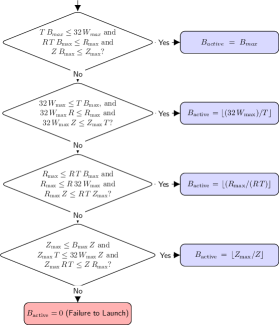
Figure 1. Rational program (presented as a flow chart) for the calculation of hardware occupancy in CUDA.

2.1. Examples

Example 0.

Hardware occupancy, as defined in the CUDA programming model, is a measure of how effective a program is making use of the hardware’s processors (Streaming Multiprocessors in case of GPUs). Hardware occupancy is calculated from hardware parameters, namely:

the maximum number $R_{\rm max}$ of registers per thread block,

the maximum number $Z_{\rm max}$ of shared memory words per thread block,

the maximum number $T_{\rm max}$ of threads per thread block,

the maximum number $B_{\rm max}$ of thread blocks per Streaming Multiprocessor (SM) and

the maximum number $W_{\rm max}$ of warps per SM, as well as low-level performance metrics, namely:

the number $R$ of registers used per thread and

the number $Z$ of shared memory words used per thread block, and a program parameter, namely the number $T$ of threads per thread block. The hardware occupancy of a CUDA kernel is defined as the ratio between the number of active warps per SM and the maximum number of warps per SM, namely $W_{\rm active}/W_{\rm max}$, where

(1) $$W_{\rm active}=\min\left(\lfloor B_{\rm active}T/32\rfloor,W_{\rm max}\right)$$

and $B_{\rm active}$ is given as a flow chart by Figure 1. Figure 1 shows how one can derive a rational program computing $B_{\rm active}$ from $R_{\rm max}$, $Z_{\rm max}$, $T_{\rm max}$, $B_{\rm max}$, $W_{\rm max}$, $R$, $Z$, $T$. It follows from Equation (1) that $W_{\rm active}$ can also be computed by a rational program from $R_{\rm max}$, $Z_{\rm max}$, $T_{\rm max}$, $B_{\rm max}$, $W_{\rm max}$, $R$, $Z$, $T$. Finally, the same is true for the hardware occupancy of a CUDA kernel.

Example 0.

The execution time of a GPU kernel is defined in the MWP-CWP execution model, see (Hong and Kim, 2009; Sim et al., 2012), and calculated from hardware parameters including:

clock frequency of a SM,

the number of SMs on the device, etc., as well as low-level performance metrics, including:

the total number $\#{\rm Mem\_insts}$ of memory instructions per thread,

the total number $\#{\rm Comp\_inst}$ of computation instructions per thread, etc., and a program parameter, namely the number $T$ of threads per thread block. We have implemented this model in the C programming language, see Section 4. This program computes the execution time (variable clockcycles) as a function of the hardware parameters, low-level performance metrics, and program parameters considered by the MWP-CWP execution model.

3. Technique Principle

3.1. Key observations

Section 3.3 presents a technique for constructing a rational program ${\mathcal{}R}$ in $P_{1},\ldots,P_{p}$, $D_{1},\ldots,D_{d}$ evaluating ${\mathcal{}E}$. This technique is based on the following two observations. The first one is a general remark about rational programs while the second one is specific to rational programs estimating performance metrics.

Observation 1.

Let ${\mathcal{}S}$ be a rational program in $X_{1},\ldots,X_{n}$ evaluating $Y$. Let $s$ be any instruction of ${\mathcal{}S}$ other than a branch or an integer part instruction. Hence, this instruction can be of the form $Z=-U$, $Z=U+V$, $Z=U-V$, $Z=U\times V$, where $U$ and $V$ can be any machine-representable rational numbers. Let $V_{1},\ldots,V_{v}$ be the variables that are defined at the entry point of the basic block of the instruction $s$. An elementary proof by induction yields the following fact. There exists a rational function in $V_{1},\ldots,V_{v}$ that we denote by $f_{s}(V_{1},\ldots,V_{v})$ such that $Z=f_{s}(V_{1},\ldots,V_{v})$ for all possible values of $V_{1},\ldots,V_{v}$.

From there, one derives the following observation. There exists a partition ${\mathcal{}T}=\{T_{1},T_{2},\ldots\}$ of ${\mbox{${\mathbb{Q}}$}}^{n}$ (where ${\mathbb{Q}}$ denotes the field of rational numbers) and rational functions $f_{1}(X_{1},\ldots,X_{n})$, $f_{2}(X_{1},\ldots,X_{n})$, …such that, if $X_{1},\ldots,X_{n}$ receive respectively the values $x_{1},\ldots,x_{n}$, then the value of $Y$ returned by ${\mathcal{}S}$ is one of $f_{i}(x_{1},\ldots,x_{n})$ where $i$ is such that $(x_{1},\ldots,x_{n})\in T_{i}$ holds. In other words, ${\mathcal{}S}$ computes $Y$ as a piece-wise rational function. Figure 1 shows that the hardware occupancy of a CUDA kernel is given as a piece-wise rational function in the variables $R_{\rm max}$, $Z_{\rm max}$, $T_{\rm max}$, $B_{\rm max}$, $W_{\rm max}$, $R$, $Z$, $T$. Hence, in this example, we have $n=8$. Moreover, Figure 1 shows that its partition of ${\mbox{${\mathbb{Q}}$}}^{n}$ contains 5 parts.

Observation 2.

It is natural to assume that low-level performance metrics depend rationally on program parameters and data parameters. While this latter fact is not explicitly discussed in the CUDA and MWP-CWP models, it is an obvious observation for very similar models which are based on the Parallel Random Access Machine (PRAM) (Stockmeyer and Vishkin, 1984; Gibbons, 1989), including PRAM-models tailored to GPU code analysis such as TMM (Ma et al., 2014) and MCM (Haque et al., 2015).

Given our assumption that the high-level performance metric ${\mathcal{}E}$ is computable as a rational program depending on hardware parameters, low-level performance metrics, and program parameters, we can therefore assume that ${\mathcal{}E}$ can be expressed as a rational program of the hardware parameters, the program parameters, and the data parameters. That is, we replace the direct dependency on low-level metrics with a dependency on the data and program parameters. Moreover, when applied to the multithreaded program ${\mathcal{}P}$ to be executed on a particular multiprocessor, we can assume that ${\mathcal{}E}$ can be expressed as a rational program depending only on program and data parameters.

3.2. Consequences

Consequence 1.

It follows from Observation 2 that we can use the MWP-CWP performance model on top of CUDA (see Examples 2 and 3) to determine a rational program estimating ${\mathcal{}E}$ depending on only program parameters and data parameters. Recall that building such a rational program ${\mathcal{}R}$ is our goal. Once ${\mathcal{}R}$ is known, it can be used at runtime (that is, when the program ${\mathcal{}P}$ is run on specific input data) to compute optimal values for the program paramters $P_{1},\ldots,P_{p}$ .

Consequence 2.

Observation 1 suggests an approach for determining ${\mathcal{}R}$. Suppose that a flow chart ${\mathcal{}C}$ representing ${\mathcal{}R}$ is partially known; to be precise, suppose that the decision nodes are known (that is, mathematical expressions defining them are known) while the process nodes are not. From Observation 1, each process node that includes no integer part instructions is given by a series of rational functions. Determining each of those rational functions can be achieved by solving an interpolation or curve fitting problem. Knowing that a function to-be-determined is rational allows us to perform parameter estimation techniques (e.g. the method of least squares) to define the fitting curve and thus the rational function.

Consequence 3.

In the above consequence, one could even consider relaxing the assumption that the decision nodes are known. Indeed, each decision node is given by a series of rational functions. Hence, those could be determined by solving curve fitting problems as well. However, we shall not discuss this direction further since this is not needed in the proposed technique presented in Sections 3.3 and 4.

3.3. Algorithm

In this section, the notations and hypotheses are the same as in Sections 2, 3.1 and 3.2. In particular, we assume that:

${\mathcal{}E}$ is a high-level performance metric for the multithreaded program ${\mathcal{}P}$ (e.g. execution time, memory consumption, and hardware occupancy),

${\mathcal{}E}$ is given (by a program execution model, e.g. CUDA or MWP-CWP) as a rational program depending on hardware parameters $H_{1},\ldots,H_{h}$, low-level performance metrics $L_{1},\ldots,L_{\ell}$, and program parameters $P_{1},\ldots,P_{p}$ (see Examples 2 and 3),

the values of the hardware parameters are known at compile-time for ${\mathcal{}P}$ while the values of the data parameters $D_{1},\ldots,D_{d}$ are known at runtime for ${\mathcal{}P}$,

the data and program parameters take integer values. Extending $(iv)$ we further assume that the possible values of the program parameters $P_{1},\ldots,P_{p}$ belong to a finite set $F\,\subset\,\mathbb{Z}^{p}$. That is to say, the possible values of ($P_{1},\ldots,P_{p}$) are a tuple of the form $(\pi_{1},\ldots,\pi_{p})\in F$, with each $\pi_{i}$ being an integer. Due to the nature of program parameters they are not necessarily all free variables (i.e. a program parameter may depend on the value of another program parameter). See Section 4 for such an example.

Following Consequence 1, we can compute a rational program ${\mathcal{}R}$ estimating ${\mathcal{}E}$ as a function of $D_{1},\ldots,D_{d}$ and $P_{1},\ldots,P_{p}$. To do so, we shall first compute rational functions $g_{1}(D_{1},\ldots,D_{d},P_{1},\ldots,P_{p})$, …, $g_{\ell}(D_{1},\ldots,D_{d},P_{1},\ldots,P_{p})$, estimating $L_{1},\ldots,L_{\ell}$ respectively. Once ${\mathcal{}R}$ has been computed, it can be used when ${\mathcal{}P}$ is being executed (thus at runtime) in order to determine optimal values for $P_{1},\ldots,P_{p}$, on given values of $D_{1},\ldots,D_{d}$. The entire process is decomposed below into six steps: the first three take place at compile-time while the other three are performed at runtime.

1. Data collection: In order to determine each of the rational functions

   $$g_{1}(D_{1},\ldots,D_{d},P_{1},\ldots,P_{p}),\ldots,g_{\ell}(D_{1},\ldots,D_{d},P_{1},\ldots,P_{p})$$

   by solving a curve fitting problem, we proceed as follows:

2. we select a set of points $K_{1},\ldots,K_{k}$ in the space of the possible values of $(D_{1},\ldots,D_{d}$, $P_{1},\ldots,P_{p})$;

3. we run (or emulate) the program ${\mathcal{}P}$ at each point $K_{1},\ldots,K_{k}$ and measure the low-level performance metrics $L_{1},\ldots,L_{\ell}$; and

4. for each $1\leq i\leq{\ell}$, we record the values $(v_{i,1},\ldots,v_{i,k})$ measured for $L_{i}$ at the respective points $K_{1},\ldots,K_{k}$.

5. Rational function estimation: For each $1\leq i\leq{\ell}$, we use the values $(v_{i,1},\ldots,v_{i,k})$ measured for $L_{i}$ at the respective points $K_{1},\ldots,K_{k}$ to estimate the rational function $g_{i}(D_{1},\ldots,D_{d},P_{1},\ldots,P_{p})$. We observe that if $v_{i,1},\ldots,v_{i,k}$ were known exactly (that is, without error) the rational function $g_{i}(D_{1},\ldots,D_{d},P_{1},\ldots,P_{p})$ could be determined exactly via rational function interpolation. However, in practice, the values $v_{i,1},\ldots,v_{i,k}$ are likely to be “noisy”. Hence, techniques from numerical analysis, like the method of least squares, must be used instead. Consequently, we compute a rational function $\hat{g_{i}}(D_{1},\ldots,D_{d},P_{1},\ldots,P_{p})$ which approximates $g_{i}(D_{1},\ldots,D_{d},P_{1},\ldots,P_{p})$ when evaluated at the points $K_{1},\ldots,K_{k}$.

6. Code generation: In order to generate the rational program ${\mathcal{}R}$, we proceed as follows:

7. we convert the rational program representing ${\mathcal{}E}$ into code, say in the C programming language, essentially encoding the CFG for computing $\mathcal{}{E}$;

8. we convert each of $\hat{g_{i}}(D_{1},\ldots,D_{d},P_{1},\ldots,P_{p})$, (for $1\leq i\leq{\ell}$) into code as well, more precisely, into sub-routines evaluating $L_{1},\ldots,L_{\ell}$, respectively; and

9. we include those sub-routines into the code computing ${\mathcal{}E}$, which yields the desired rational program ${\mathcal{}R}$.

10. Rational program evaluation: At this step, the rational program ${\mathcal{}R}$ is completely determined and can be used when the program ${\mathcal{}P}$ is executed. At the time of execution, the data parameters $D_{1},\ldots,D_{d}$ are given particular values, say ${\delta}_{1},\ldots,{\delta}_{d}$, respectively. For those specified values of $D_{1},\ldots,D_{d}$ and for all practically meaningful values of $P_{1},\ldots,P_{p}$ from the set $F$, we compute an estimate of ${\mathcal{}E}$ using ${\mathcal{}R}$. Here, “practically meaningful” refers to the fact that the values of the program parameters $P_{1},\ldots,P_{p}$ are likely to be constrained by the values of the data parameters $D_{1},\ldots,D_{d}$. For instance, if $P_{1},P_{2}$ are the two dimension sizes of a two-dimensional thread-block of a CUDA kernel performing the transposition of a square matrix of order $D_{1}$, then the inequality $P_{1}P_{2}\leq D_{1}^{2}$ is meaningful. Despite of this remark, this step can still be seen as an exhaustive search, and, it is practically feasible to do so for three reasons:

11. $p$ is small, typically $p=1$, $p=2$ or $p=3$, see Section 4;

12. the set of values in $F$ are small (typically on the order of 10 elements in case of MWP-CWP model); and

13. the program ${\mathcal{}R}$ simply evaluates a few formulas and thus runs almost instantaneously.

14. Selection of optimal values of program parameters: In general, when the search space of values of the program parameters $P_{1},\ldots,P_{p}$ is large, a numerical optimization technique is required for this step. For CUDA kernels, however, selecting a value point (also called a configuration in the rest of this report) which is optimal can be done with an exhaustive search, as seen in the previous step, and is hence trivial. The only possible challenge in this case is that several configurations may optimize ${\mathcal{}E}$. When this happens, using a second performance metric can help refine the choice of a best configuration.

15. Program execution: Once a best configuration is selected, the program ${\mathcal{}P}$ can finally be executed using this configuration of program parameters $P_{1},\ldots,P_{p}$ along with with the values ${\delta}_{1},\ldots,{\delta}_{d}$ of $D_{1},\ldots,D_{d}$.

4. Implementation

In the previous sections we gave an overview of our technique for general multithreaded programs $\mathcal{}{P}$. For the embodiment of this technique, and the resulting experimentation and performance analysis, we focus on programs for GPU architectures using the programming model CUDA. These programs interleave (i) serial code which is executed on the host (the CPU) and, multithreaded code which is executed on the device (the GPU). The host launches a device code execution by calling a particular type of function, called a kernel. Optimizing a CUDA program for better usage of the computing resources on a device essentially means optimizing each of its kernels. Therefore, we apply the ideas of Sections 3.1 through 3.3 to CUDA kernels.

In the case of a CUDA kernel the data parameters are a description of the input data size. In many examples this is a single parameter, say $N$, describing the size of an array (or the order of a two-dimensional array), the values of which are usually powers of $2$. On the other hand, the program parameters are typically an encoding of the program configuration, namely the thread block configuration. In CUDA the thread block configuration defines both the number of dimensions (1, 2, or 3) and the size in each dimension of each thread block — a contiguous set of threads mapped together to a single SM processor. For example, a possible thread block configuration may be $1024\times 1\times 1$ (a one-dimensional thread block), or $16\times 16\times 2$ (a three-dimensional thread block). In all cases the CUDA model restricts the number of threads per block (i.e. the product of the size in each dimension) to be $1024$ on devices of Compute Capability (CC) 2.x, or newer. This limits the possible thread block configurations, and, moreover, limits the set $F$ from which the program parameters are chosen.

Throughout the current and the following sections our discussions make use of these specialized terms, input data size and thread block configuration, for data and program parameters, respectively, in order to make clear explanations and associations between theory and practice.

4.1. Data collection

As detailed in Step 1 of Section 3.3, we must collect data and statistics regarding certain performance counters and runtime metrics (which are thoroughly defined in (Hong and Kim, 2009) and (cud, 2018a)). These metrics together allow us to estimate the execution time of the program and can be partitioned into three categories.

First, we need architecture-specific performance counters, basically, characteristics dictated by the CC of the target device. Such hardware characteristics can be obtained at compile time, as the target CC is specified at this time. These characteristics include the number of registers used in each thread, the amount of static shared memory per thread block, and the number of (arithmetic, memory, and synchronization) instructions per thread. This information can easily be obtained from a CUDA compiler (e.g. NVIDIA’s NVCC).

Second, we have the values that depend on the behavior of the kernel code at runtime which we will refer to as kernel-specific runtime values. This includes values impacted by memory access patterns, namely, the number of coalesced and non-coalesced memory accesses per warp, the number of memory instructions in each thread that cause coalesced and non-coalesced accesses, and eventually, the total number of warps that are being executed. For this step we have two choices. We can use an emulator, which can mimic the behavior of a GPU on a typical Central Processing Unit (CPU). This is important if we cannot guarantee that a device is available at compile time. For this purpose, we have configured Ocelot (Diamos et al., 2010), a dynamic compilation framework for GPU computing as well as an emulator for low-level CUDA (PTX (cud, 2018b)) code, to meet our needs. Alternatively, we can use a profiler to collect the required metrics on an actual device. For this solution, we have used NVIDIA’s nvprof(Corporation, 2019b).

Third, in order to compute a more precise estimate of the clock cycles, we need device-specific parameters which describe an actual GPU card. One subset of such parameters can be determined by microbenchmarking the device (see (Mei and Chu, 2017) and (Wong et al., 2010)), this includes the memory latency, the memory bandwidth, and the departure delay for coalesced/non-coalesced accesses. Another subset of such parameters can be easily obtained by consulting the vendor’s guide (Corporation, 2019a), or by querying the device itself via the CUDA API. This includes the number of SMs on the card, the clock frequency of SM cores, and the instruction delay.

In summary, our general method proceeds as follows:

Beginning with a CUDA program, we minimally annotate the host code to make it compatible with our pre-processor program, specifying the code fragment in the host code which calls the kernel. We also specify the CC of the target device.

The pre-processor program prepares the code for collecting kernel-specific runtime values. This step includes source code analysis in order to extract the list of kernels, the list of kernel calls in the host code, and finally, the body of each kernel (which will be used for further analysis). In the case of Ocelot emulation, the pre-processor replaces the device kernel calls with equivalent Ocelot kernel calls, while in the case of actual profiling, the device kernel calls are left untouched. Finally, the pre-processor program uses the specified CC in the host code to determine the architecture-specific performance counters for each kernel. The result of this step is an executable file, which we will refer to as the instrumentor. The instrumentor takes as input the same program parameters as the original CUDA code.

A driver program orchestrates the combination of device-specific characteristics (i.e. a device profile) and various configurations of program and data parameters to be passed to the instrumentor. Running the instrumentor (either emulated on top of Ocelot, or running via a profiler on a GPU) measures and records the required performance metrics.

4.2. Rational function estimation

Once data collection is completed, we are able to move on to the estimation step, see Step 2 of Section 3.3. That is, determining precisely the rational functions $f_{b}(X_{1},\dots,X_{n})$, for each desired code block $b$, which are to be used within the rational program (see Section 2). These $X_{i}$ variables are simply combinations of program parameters, data parameters, and intermediate values, obtained during the execution of the rational program. These intermediate values are, in turn, are rational functions of the program and data parameters. Hence, the variables $X_{1},\dots,X_{n}$ are used only to simplify notations.

$$f_{b}(X_{1},\dots,X_{n}) =\frac{p_{b}(X_{1},\dots,X_{n})}{q_{b}(X_{1},\dots,X_{n})}$$

$$=\frac{\alpha_{1}\cdot(X_{1}^{0}\dots X_{n}^{0})\;+\;\dots\;+\;\alpha_{i}\cdot(X_{1}^{u_{1}}\dots X_{n}^{u_{n}})}{\beta_{1}\cdot(X_{1}^{0}\dots X_{n}^{0})\;+\;\dots\;+\;\beta_{j}\cdot(X_{1}^{v_{1}}\dots X_{n}^{v_{n}})}$$

A rational function is simply a fraction of two polynomials. With a degree bound (an upper limit on the exponent) on each variable $X_{k}$ in the numerator and the denominator, say $u_{k}$ and $v_{k}$, respectively, these polynomials can be defined up to some parameters, namely the coefficients of the polynomials, say $\alpha_{1},\dots,\alpha_{i}$ and $\beta_{1},\dots,\beta_{j}$.

Using the previously collected data (see Section 4.1) we perform a parameter estimation (for each rational function) on the polynomial coefficients $\alpha_{1},\ldots,\alpha_{i},\beta_{1},\ldots,\beta_{j}$. in order to uniquely determine the rational function. We note that while our model is non-linear, it is indeed linear in the model-fitting parameters $\alpha_{1},\ldots,\alpha_{i},\beta_{1},\ldots,\beta_{j}$.

The system of linear equations defined by the model-fitting parameters $\alpha_{1},\ldots,\alpha_{i},\beta_{1},\ldots,\beta_{j}$ can very classically be defined as an equation of the form $\mathbf{Ax}=\mathbf{b}$, where $\mathbf{A}\in\mathbb{R}^{m\times n}$ (the sample matrix) and $\mathbf{b}\in\mathbb{R}^{m\times 1}$ (the right-hand side vector) encode the collected data, while the solution vector $\mathbf{x}\in\mathbb{R}^{n\times 1}$ encodes the model-fitting parameters. An exact solution is rarely defined if $m<n$ (where an infinite number of solutions is possible) or if $m>n$. Therefore, we wish to get a solution in the “least squares sense”, that is, find $\mathbf{x}$ such that residual is minimized:

$$\mathbf{x}\>=\>\min_{\mathbf{x}}||\mathbf{r}||^{2}_{2}\>=\>\min_{\mathbf{x}}||\mathbf{b}-\mathbf{Ax}||_{2}^{2}$$

Many different methods exist for solving this so-called linear least squares problem, such as the normal-equations, or QR-factorization, however, these methods are either numerically unstable (normal-equations), or will fail if the sample matrix is rank-deficient (both normal-equations and QR) (Corless and Fillion, 2013). We rely then on the singular value decomposition (SVD) of $\mathbf{A}$ to solve this problem. This decomposition is very computationally intensive, much more than that of normal-equations or QR, but is also much more numerically stable, as wel as being capable of producing solutions with a rank-deficient sample matrix.

We are highly concerned with the robustness of our method due to three problems present in our particular situation:

1. the sample matrix is very ill-conditioned;

2. the sample matrix will often be (numerically) rank-deficient;

3. we are interested in using our fitted model for extrapolation, meaning any numerical error in the model fitting will grow very quickly (Corless and Fillion, 2013).

While (3) is an issue inherent to our model fitting problem, (1) and (2) result from our choice of model, and how the sample points $(X_{1},\ldots,X_{n})$ are chosen, respectively. Using a rational function (or polynomial) as the model for which we wish to estimate parameters presents numerical problems. The resulting sample matrix is essentially a Vandermonde matrix. These matrices, while theoretically of full rank, are extremely ill-conditioned (Corless and Fillion, 2013; Beckermann, 2000). To discuss (2) we must now consider the so-called “poised-ness” of the sample points.

For a univariate polynomial model, a sample matrix is guaranteed to have full rank if the sample points are all distinct. We say that the points producing the sample matrix are poised is the matrix is of full rank. In the multivariate case, it is much more difficult to make such a guarantee (Chung and Yao, 1977; Olver, 2006). Given a multivariate polynomial model with a total degree $d$, a set of points is poised if, for each point $x_{i}$, there exists $d$ hyperplanes corresponding to this point such that all other points lie on at least one of these hyperplanes but $x_{i}$ does not (Chung and Yao, 1977). For example, with 2 variables and a total degree 3, the sample points are poised if, for each sample point, there exists 3 lines on which all other points lie but the selected point does not.

This geometric restriction on sample points is troublesome for our purposes. For example, if we are trying to model a function which has, in part, CUDA thread block dimensions as variables, then these dimensions should be chosen such that their product is a multiple of 32 (Ryoo et al., 2008a). However, this corresponds very closely with the geometric restriction we are trying to avoid. Consider the possible 2D thread block dimensions ($B_{0},B_{1}$) for a CUDA kernel (Figure 2). Many subsets of these points are collinear, presenting challenges for obtaining poised sample points. As a result of all of this we are highly likely to obtain a rank-deficient sample matrix.

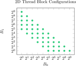
Figure 2. Possible 2D thread block configurations for a CUDA kernel.

Despite all of these challenges our parameter estimation techniques are well-implemented in optimized C code. We use optimized algorithms from LAPACK (Linear Algebra PACKage) (Anderson et al., 1999) for singular value decomposition and linear least squares solving while rational function and polynomial implementations are similarly highly optimized thanks to the Basic Polynomial Algebra Subprograms (BPAS) library (Asadi et al., 2018; Brandt, 2018). With parameter estimation complete the rational functions required for the rational program are fully specified and we can finally construct it.

4.3. Rational programs

In practice, the use of rational programs is split into two parts: the generation of the rational program at the compile-time of the multithreaded program $\mathcal{}{P}$, and the use of the rational program during the runtime of $\mathcal{}{P}$.

4.3.1. Compile-time code generation

We are now at Step 3 of Section 3.3. We look to define a rational program which evaluates the high-level metric $\mathcal{}{E}$ of the program $\mathcal{}{P}$ using the MWP-CWP model. In implementation, this is achieved by using a previously defined rational program template which contains the formulas and case discussion of the MWP-CWP model, independent of the particular program being investigated. Using simple regular expression matching and text manipulation we combine the rational program template with the rational functions determined in the previous step to obtain a rational program specialized to the multithreaded program $\mathcal{}{P}$. The generation of this rational program is performed completely during compile-time, before the execution of the program itself.

4.3.2. Runtime optimization

At runtime, the input data sizes (data parameters) are well known. In combination with the known hardware parameters, since the program is actually being executed on a specific device, we are able to specialize every parameter in the rational program and obtain an estimate for the high-level metric $\mathcal{}{E}$. This rational program is then easily and quickly evaluated during (or immediately prior to) the execution of $\mathcal{}{P}$. Evaluating the rational program for each possible thread block configuration, as restricted by our data parameters and the CUDA programming model itself, we determine a thread block configuration which optimizes $\mathcal{}{E}$. The program $\mathcal{}{P}$ is finally executed using this optimal thread block configuration. Therefore, we have completed Steps 4 to 6 of Section 3.3.

5. Experimentation

In this section we highlight the performance and experimentation of our technique applied to example CUDA programs from the PolyBench benchmarking suite (Grauer-Gray and Pouchet, 2012). For each PolyBench example, we collect statistical data (see Section 4) with various input sizes $N$ (powers of 2 typically between 64 and 512). These are relatively small sizes to allow for fast data collection. The collected data is used to produce the rational functions and, lastly, the rational functions are combined to form the rational programs. Table 1 gives a short description for each of the benchmark examples, as well as an index for each kernel which we use for referring to that kernel in the experimental results.

The ability of the rational programs we generate to effectively optimize the program parameters of each example CUDA program is summarized in Tables 2 and 3. The definitions of the notations used in these tables are as follows:

$N$: the input size of the problem, usually a power of 2,

$Ec$: estimated execution time of the kernel measured in clock-cycles,

$C_{r}$: best thread block configuration as decided by the rational program,

$C_{d}$: default thread block configuration given by the benchmark,

$Ec_{r}$: $Ec$ of configuration $C_{r}$ as decided by the rational program,

$C_{i}$: best thread block configuration as decided by instrumentation,

$Ec_{i}$: $Ec$ of configuration $C_{i}$ as decided by instrumentation,

Best_time (B_t): the best CUDA running time (i.e. the time to actually run the code on a GPU) of the kernel among all possible configurations,

Worst_time (W_t): the worst CUDA running time of the kernel among all possible configurations.

To evaluate the effectiveness of our rational program, we compare the results obtained from it with an actual analysis of the program using the performance metrics collected by the instrumentor. This comparison gives us estimated clock cycles as shown in Table 2. The table shows the best configurations ($C_{i}$ and $C_{r}$) for $N=256$ and $N=512$ for each example, as decided from both the data collected during instrumentation and the resulting rational program. This table is meant to highlight that the construction of the rational program from the instrumentation data is performed correctly. Here, either the configurations should be the same or, if they differ, then the estimates of the clock-cycles should be very similar; indeed, it is possible that different thread block configurations (program parameters) result in the same execution time. Hence, the rational program must choose one of the possibly many optimal configurations. Moreover, we supply the value “Collected $Ec$” which gives the $Ec$ given by the instrumentation for the thread block configuration $C_{r}$. This value shows that the rational program is correctly calculating $Ec$ for a given thread block configuration. The values “Collected $Ec$” and $Ec_{r}$ should be very close.

Figure 3 illustrates detailed results for Kernel 8.2 when $N=512$. The “CUDA” plot shows the real runtime of the kernel launched on a device while the “RP-Estimated” plot shows the estimates obtained from our rational program. The $x$ axis shows the various thread block configurations. The runtime values on $y$ axis are normalized to values between $0$ and $100$.

Table 3 shows the best configuration ($C_{r}$) for $N=1024$ and $N=2048$ estimated by the rational program of each example. Notice these values of $N$ are much larger than those used during the instrumentation and construction of the rational program. This shows that the rational program can extrapolate on the data used for its construction and accurately estimate optimal program parameters for different data parameters. To compare the thread block configuration deemed optimal by the rational program ($C_{r}$) and the optimal thread block configuration determined by actually executing the program with various thread block configurations we calculate the value named “Error”. This is a percentage given by ($C_{r}t$ - Best_time)/(Worst_time - Best_time) * 100%, where “$C_{r}t$” is the actual running time of the program using the thread block configuration $C_{r}$ in millisecond. Best_time and Worst_time are as defined above. The error percentage shows the quality of our estimation; it clearly shows the difference between the estimated configuration and the actual best configuration. This percentage should be as small as possible to indicate a good estimation.

As an exercise in the practicality of our technique, we also show the default thread block configuration ($C_{d}$) given by the benchmarks and “$C_{d}t$”, the actual running time of the program using the thread block configuration $C_{d}$ in the same table. Compared to the default configurations, the rational program determines a better configuration for more than half of the kernels. Notice that, in most cases, the same default configuration is used for all kernels within a single example. In contrast, our rational program can produce different configurations optimized for each kernel individually.

As mentioned in Section 4.1, we use both Ocelot (Diamos et al., 2010) and NVIDIA’s nvprof(Corporation, 2019b) as instrumentors in the data collection step. The “Error” of the implementation based on data collected by Ocelot is shown in the column “Ocel” in Table 3. We can see that the overall performance is better with nvprof, but for some benchmarks, for example Kernel 12, the best configuration picked by the rational program is not as expected. We attribute this to the limitations of the underlying MWP-CWP model we use.

More experimental results may be found on our GitHub repository: https://github.com/orcca-uwo/Parametric_Estimation/tree/master/plots

Benchmark	Description	Kernel name	Kernel ID
2D Convolution	2-D convolution	Convolution2D_kernel	$1$
FDTD_2D	2-D Finite Different	fdtd_step1_kernel	$2.1$
	Time Domain	fdtd_step2_kernel	$2.2$
		fdtd_step3_kernel	$2.3$
2MM	2 Matrix Multiplications	mm2_kernel1	$3$
3MM	3 Matrix Multiplications	mm3_kernel1	$4$
BICG	BiCGStab Linear Solver	bicg_kernel1	$5.1$
		bicg_kernel2	$5.2$
GEMM	Matrix Multiplication	gemm_kernel	$6$
3D_Convolution	3-D Convolution	convolution3D_kernel	$7$
ATAX	Matrix Transpose and	atax_kernel1	$8.1$
	Vector Multiplication	atax_kernel2	$8.2$
GESUMMV	Scalar, Vector and	gesummv_kernel	$9$
	Matrix Multiplication
SYRK	Symmetric rank-k operations	syrk_kernel	$10$
MVT	Matrix Vector Product and	mvt_kernel1	$11.1$
	Transpose	mvt_kernel2	$11.2$
SYR2K	Symmetric rank-2k operations	syr2k_kernel	$12$
CORR	Correlation Computation	corr_kernel	$13.1$
		mean_kernel	$13.2$
		reduce_kernel	$13.3$
		std_kernel	$13.4$
COVAR	Covariance Computation	covar_kernel	$14.1$
		mean_kernel	$14.2$
		reduce_kernel	$14.3$
GRAMSCHM	Gram-Schmidt decomposition	gramschmidt_kernel1	$15.1$
		gramschmidt_kernel2	$15.2$
		gramschmidt_kernel3	$15.3$

Table 1. Benchmark names and descriptions

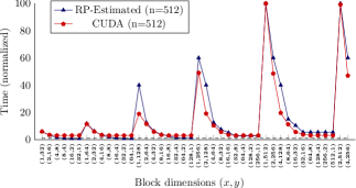
Figure 3. Example of Kernel atax_kernel2 from Polybench suite.

ID	$N$	Data collection		Rational Program
		$C_{i}$	$Ec_{i}$	$C_{r}$	$Ec_{r}$	Collected $Ec$
1	256	$16\times 2$	198070	$16\times 2$	310463	198070
	512	$16\times 4$	794084	$16\times 16$	947799	889378
2.1	256	$16\times 2$	44336	$32\times 1$	40213	44336
	512	$16\times 4$	147622	$32\times 2$	135821	147622
2.2	256	$32\times 1$	19430	$32\times 1$	52096	19430
	512	$32\times 2$	64475	$64\times 1$	135810	64475
2.3	256	$32\times 1$	19476	$16\times 2$	97964	19640
	512	$32\times 2$	64643	$16\times 4$	326474	65191
3	256	$16\times 2$	351845192	$32\times 1$	1365006816	351845192
	512	$16\times 4$	4610508174	$16\times 64$	18148896630	4610508174
4	256	$16\times 2$	351845192	$16\times 2$	1364711040	351845192
	512	$16\times 4$	4610508174	$16\times 64$	18147912950	4610508174
5.1	256	$8\times 4$	6730198	$16\times 2$	13105400	6927829
	512	$16\times 2$	27224663	$32\times 1$	56699908	28801623
5.2	256	$8\times 4$	6729688	$16\times 2$	13105400	6927319
	512	$16\times 2$	27223641	$32\times 1$	56699908	28800601
6	256	$16\times 2$	352450569	$32\times 1$	1365746112	352450569
	512	$16\times 4$	4614492176	$16\times 4$	18091801600	4614492176
7	256	$16\times 2$	412448	$8\times 4$	419355	423967
	512	$16\times 4$	1382453	$16\times 4$	1382446	1382453
8.1	256	$8\times 4$	6741283	$16\times 2$	13836355	6938145
	512	$16\times 2$	27245283	$32\times 1$	57486243	28819169
8.2	256	$8\times 4$	6741791	$16\times 2$	13836672	6938653
	512	$16\times 2$	27246303	$32\times 1$	57486880	28820189
9	256	$8\times 4$	52142036	$16\times 2$	104085531	53194198
	512	$16\times 2$	211244951	$32\times 1$	438726895	219647900
10	256	$16\times 2$	352450567	$32\times 1$	1365746112	352450567
	512	$16\times 4$	4614492172	$16\times 4$	18091801600	4614492172
11.1	256	$8\times 4$	6741790	$16\times 2$	13450360	6938652
	512	$16\times 2$	27246302	$32\times 1$	56715288	28820188
11.2	256	$8\times 4$	6741283	$16\times 2$	13450360	6938145
	512	$16\times 2$	27245283	$32\times 1$	56715288	28819169
12	256	$16\times 2$	1090910216	$16\times 2$	4293143808	1090910216
	512	$16\times 4$	14402949134	$32\times 16$	57121538780	14402949134
13.1	256	$8\times 4$	29762	$16\times 2$	431621481191	34578
	512	$1\times 32$	81924	$32\times 1$	7075540802475	226841
13.2	256	$8\times 4$	159563703552	$16\times 2$	5176052	222555249312
	512	$16\times 2$	3428474954532	$32\times 1$	22396088	3534048733179
13.3	256	$8\times 4$	6938660	$1\times 32$	5355	33687503
	512	$16\times 2$	28036520	$1\times 64$	22447	502559959
13.4	256	$8\times 4$	2526616	$16\times 2$	14040368	2659225
	512	$16\times 2$	10298524	$32\times 1$	58770372	11353249
14.1	256	$8\times 4$	2526616	$32\times 1$	474507050858	2924449
	512	$16\times 2$	10298524	$32\times 1$	7115480129956	11353249
14.2	256	$8\times 4$	162030833356	$16\times 2$	5147212	225920838132
	512	$16\times 2$	3454820728440	$32\times 1$	22398140	3560802413900
14.3	256	$64\times 1$	1060	$32\times 1$	1484	1069
	512	$128\times 1$	1085	$128\times 1$	1677	1085
15.1	256	$16\times 2$	77754074	$256\times 1$	70701	646426704
	512	$32\times 1$	324346910	$512\times 1$	136765	5169397920
15.2	256	$256\times 1$	68119	$8\times 4$	1871	1145070
	512	$512\times 1$	136231	$8\times 8$	1873	8409096
15.3	256	$16\times 4$	1492	$16\times 2$	78089365	1505
	512	$32\times 2$	1492	$32\times 1$	324813912	1505

Table 2. Sanity check (nvprof)

ID	$N$	Default Config		Rational Program		B_t	W_t	Error	Ocel
		$C_{d}$	$C_{d}t$	$C_{r}$	$C_{r}t$
1	1024	$32\times 8$	0.04	$32\times 8$	0.04	0.04	0.34	0.00	6.11
	2048	$32\times 8$	0.16	$128\times 4$	0.16	0.15	1.31	0.86	6.43
2.1	1024	$32\times 8$	18.2	$32\times 1$	23.4	18.1	84.0	7.93	0.06
2.2	1024	$32\times 8$	19.9	$64\times 2$	19.7	19.5	82.3	0.26	0.04
2.3	1024	$32\times 8$	25.7	$16\times 2$	27.2	25.7	109	1.79	0.02
3	1024	$32\times 8$	5.73	$16\times 2$	9.67	5.73	89.0	4.73	0.57
	2048	$32\times 8$	46.7	$16\times 2$	78.6	46.7	707	4.83	1.10
4	1024	$32\times 8$	5.77	$16\times 2$	9.68	5.73	89.8	4.69	0.63
	2048	$32\times 8$	47.3	$16\times 2$	78.8	47.1	731	4.63	1.30
5.1	1024	$256\times 1$	0.25	$32\times 1$	0.25	0.25	9.27	0.01	0.08
	2048	$256\times 1$	0.51	$32\times 1$	0.50	0.50	37.2	0.00	1.10
5.2	1024	$256\times 1$	0.19	$32\times 1$	0.18	0.16	9.48	0.17	0.00
	2048	$256\times 1$	0.38	$32\times 1$	0.36	0.36	38.5	0.01	0.02
6	1024	$32\times 8$	5.76	$32\times 1$	9.69	5.76	95.6	4.37	0.02
	2048	$32\times 8$	46.3	$32\times 1$	78.3	46.3	725	4.70	1.26
7	1024	$32\times 8$	56.0	$8\times 4$	81.6	55.2	369	8.38	1.49
8.1	1024	$256\times 1$	0.20	$32\times 1$	0.19	0.17	9.87	0.15	0.36
	2048	$256\times 1$	0.39	$32\times 1$	0.37	0.37	42.5	0.00	0.28
8.2	1024	$256\times 1$	0.26	$32\times 1$	0.24	0.24	9.35	0.03	0.42
	2048	$256\times 1$	0.50	$32\times 1$	0.49	0.49	40.3	0.01	0.67
9	1024	$256\times 1$	0.40	$32\times 1$	0.37	0.34	2.10	1.53	1.04
	2048	$256\times 1$	0.80	$32\times 1$	0.74	0.73	6.32	0.08	0.44
10	1024	$32\times 8$	0.02	$32\times 1$	34.3	17.9	87.9	23.38	0.00
	2048	$32\times 8$	239	$32\times 1$	968	143	2802	31.03	1.39
11.1	1024	$256\times 1$	0.20	$32\times 1$	0.19	0.17	9.83	0.17	0.00
	2048	$256\times 1$	0.39	$32\times 1$	0.38	0.36	39.3	0.03	0.03
11.2	1024	$256\times 1$	0.25	$32\times 1$	0.24	0.24	9.55	0.02	0.05
	2048	$256\times 1$	0.50	$32\times 1$	0.49	0.49	37.4	0.00	0.15
12	1024	$32\times 8$	90.5	$32\times 1$	338	32.0	338	100.0	0.25
	2048	$32\times 8$	2295	$32\times 1$	5276	251	6723	77.64	0.89
13.1	1024	$256\times 1$	320	$8\times 8$	256	224	2461	1.42	0.00
	2048	$256\times 1$	1359	$1\times 128$	7410	1186	18361	36.23	0.63
13.2	1024	$256\times 1$	0.26	$32\times 1$	0.26	0.25	1.98	0.17	6.21
	2048	$256\times 1$	0.52	$32\times 1$	0.51	0.51	7.22	0.00	1.85
13.3	1024	$32\times 8$	0.05	$1\times 128$	0.02	0.02	0.21	0.00	3.02
	2048	$32\times 8$	0.21	$1\times 128$	0.10	0.10	0.85	0.13	0.46
13.4	1024	$256\times 1$	0.26	$32\times 1$	0.25	0.25	2.18	0.15	0.09
	2048	$256\times 1$	0.53	$32\times 1$	0.52	0.52	8.16	0.00	1.43
14.1	1024	$256\times 1$	1065	$32\times 8$	394	226	2462	7.54	0.00
	2048	$256\times 1$	2116	$64\times 16$	6119	1182	18343	28.76	7.18
14.2	1024	$256\times 1$	1.63	$64\times 1$	0.26	0.25	2.30	0.39	0.11
	2048	$256\times 1$	3.29	$32\times 1$	0.51	0.51	7.58	0.05	1.39
14.3	1024	$32\times 8$	0.03	$128\times 1$	0.01	0.01	1.48	0.00	0.07
	2048	$32\times 8$	0.11	$128\times 1$	0.01	0.01	5.94	0.00	0.00
15.1	1024	$256\times 1$	17.3	$512\times 1$	17.5	17.1	23.1	7.27	6.91
	2048	$256\times 1$	82.8	$512\times 1$	83.1	82.7	87.3	7.98	24.15
15.2	1024	$256\times 1$	3.03	$64\times 1$	2.93	2.93	4.34	0.00	27.98
	2048	$256\times 1$	6.53	$32\times 1$	6.64	6.36	11.5	5.47	24.56
15.3	1024	$256\times 1$	389	$32\times 1$	375	375	522	0.00	10.42
	2048	$256\times 1$	2000	$32\times 1$	1947	1944	3818	0.11	8.63

Table 3. Proof of Concept (nvprof)

6. Related work

We briefly review a number of previous works on the performance estimation of parallel programs in the context of GPUs and CUDA programming model. Ryoo et al (Ryoo et al., 2008b) present a performance tuning approach for general purpose applications on GPUs which is limited to pruning the optimization space of the applications and lacks support for memory-bound cases. Hong et al (Hong and Kim, 2009) describe an analytical model that estimates the execution time of GPU kernels. They use this model to identify the performance bottlenecks (via static analysis and emulation) and optimize the performance of a given CUDA kernel. Baghsorkhi et al (Baghsorkhi et al., 2010) present a dynamically adaptive approach for modeling performance of GPU programs which relies on dynamic instrumentation of the program at the cost of adding runtime overheads. This model cannot statically determine the optimal program parameters at compile time. In (Lim et al., 2017) the authors claim to have a static analysis method which does not require running the code for determining the best configuration for CUDA kernels. They analyze the assembly code generated by the NVCC compiler and estimate the IPC of each instruction, but, there is no analysis of memory access pattern. The authors assume that each CUDA kernel consists of a for-loop nest and that the execution time is proportional to the input problem size. These are, obviously, very strong assumptions, and impractical for real world applications. Moreover, the paper only reports on 4 test-cases (unlike a standard test suite such as PolyBench which includes 15 examples).

More recently, the author of (Volkov, 2018, 2016) has suggested a new GPU performance model which relies on Little’s law (Little, 1961), that is, measuring concurrency as a product of latency and throughput. The suggested model takes both warp and instruction concurrency into account. This approach stands in opposition to the common view of many models, including those of (Corporation, 2019a), (Hong and Kim, 2009), (Sim et al., 2012), and (Baghsorkhi et al., 2010), which only consider warps as the unit of concurrency. The model measures the performance in terms of required concurrency for the latency-bound cases (when occupancy is small and throughput grows with occupancy) and throughput-bound cases (when occupancy is large while throughput is at a maximum and is constant w.r.t. occupancy). The author’s analysis of models in (Corporation, 2019a; Hong and Kim, 2009; Sim et al., 2012; Baghsorkhi et al., 2010) indicates that the most common limitation among all of them is the significant underestimation of occupancy when the arithmetic intensity (number of arithmetic instructions per memory access) of the code is intermediate. Other major drawbacks include the low accuracy of the prediction when the code is memory intensive (i.e., low arithmetic intensity), and underestimation, or overestimation, of the throughput (in the case of (Baghsorkhi et al., 2010) and (Huang et al., 2014), respectively). Noticeably, the author emphasizes the importance of cusp behavior; that is, ”hiding both arithmetic and memory latency at the same time may require more warps than hiding either of them alone” (Volkov, 2016). Cusp behavior is observed in practice, however, it is not indicated in the previously mentioned performance prediction models.

7. Conclusions and Future Work

Our main objective is to provide a solution for portable performance optimization of multithreaded programs. In the context of CUDA programs, other research groups have used techniques like auto-tuning (Grauer-Gray et al., 2012; Khan et al., 2013), dynamic instrumentation (Kistler and Franz, 2003), or both (Song et al., 2015). Auto-tuning techniques have achieved great results in projects such as ATLAS (Whaley and Dongarra, 1998), FFTW (Frigo and Johnson, 1998), and SPIRAL (Püschel et al., 2004) in which part of the optimization process occurs off-line and then it is applied and refined on-line. In contrast, we propose to build a completely off-line tool, namely, the rational program.

For this purpose, we present an end-to-end novel technique for compile-time estimation of program parameters for optimizing a chosen performance metric, targeting manycore accelerators, particularly, CUDA kernels. Our method can operate without precisely knowing the numerical values of any of the data or program parameters when the optimization code is being constructed. This naturally leads to a case discussion depending on the values of those parameters, which is precisely what can be accomplished by our notion of a rational program. Moreover, our idea is verifiably extensible to any architectural additions, owing to the principle that low level performance metrics are piece-wise rational functions of data parameters, hardware parameters, and program parameters. Our approach relies on the instrumentation of the program, and collection of certain runtime values for few selected small input data sizes, to approximate the runtime performance characteristics of the program at larger input data sizes. Program instrumentations, in conjunction with source code analysis and theoretical modeling, are central to avoid costly dynamic analysis. Consequently, compilers will be able to tune applications for the target hardware at compile-time, rather than having to offload that responsibility to the end users.

As it is observed from Tables 2 and 3, our current implementation suffers from inaccuracy for certain examples. We attribute this problem to usage of the MWP-CWP of (Hong and Kim, 2009; Sim et al., 2012) as our performance prediction model. In future work, we expect that by switching to the model of (Volkov, 2018, 2016), we will be able to improve the accuracy of the rational program estimation.

Acknowledgements

The authors would like to thank IBM Canada Ltd (CAS project 880) and NSERC of Canada (CRD grant CRDPJ500717-16).

References

- (1)
- cud (2018a) 2018a. CUDA Runtime API: v10.0. NVIDIA Corporation. http://docs.nvidia.com/cuda/pdf/CUDA_Runtime_API.pdf.
- cud (2018b) 2018b. CUDA Toolkit Documentation, version 10.0. NVIDIA Corporation. https://docs.nvidia.com/cuda/.
- Aho et al. (1986) Alfred V. Aho, Ravi Sethi, and Jeffrey D. Ullman. 1986. Compilers: Principles, Techniques, and Tools. Addison-Wesley Longman Publishing Co., Inc., Boston, MA, USA.
- Anderson et al. (1999) E. Anderson, Z. Bai, C. Bischof, S. Blackford, J. Demmel, J. Dongarra, J. Du Croz, A. Greenbaum, S. Hammarling, A. McKenney, and D. Sorensen. 1999. LAPACK Users’ Guide (third ed.). Society for Industrial and Applied Mathematics, Philadelphia, PA.
- Asadi et al. (2018) Mohammadali Asadi, Alexander Brandt, Changbo Chen, Svyatoslav Covanov, Farnam Mansouri, Davood Mohajerani, Robert Moir, Marc Moreno Maza, Ning Xie, and Yuzhen Xie. 2018. Basic Polynomial Algebra Subprograms (BPAS). http://www.bpaslib.org.
- Baghsorkhi et al. (2010) Sara S. Baghsorkhi, Matthieu Delahaye, Sanjay J. Patel, William D. Gropp, and Wen-mei W. Hwu. 2010. An Adaptive Performance Modeling Tool for GPU Architectures. In Proceedings of the 15th ACM SIGPLAN Symposium on Principles and Practice of Parallel Programming (PPoPP ’10). ACM, 105–114.
- Beckermann (2000) Bernhard Beckermann. 2000. The condition number of real Vandermonde, Krylov and positive definite Hankel matrices. Numer. Math. 85, 4 (2000), 553–577.
- Brandt (2018) Alexander Brandt. 2018. High Performance Sparse Multivariate Polynomials: Fundamental Data Structures and Algorithms. Master’s thesis. University of Western Ontario, London, ON, Canada.
- Chung and Yao (1977) Kwok Chiu Chung and Te Hai Yao. 1977. On lattices admitting unique Lagrange interpolations. SIAM J. Numer. Anal. 14, 4 (1977), 735–743.
- Corless and Fillion (2013) Robert M Corless and Nicolas Fillion. 2013. A graduate introduction to numerical methods. Springer.
- Corporation (2019a) NVIDIA Corporation. 2019a. CUDA C Programming Guide, v10.1.105. {https://docs.nvidia.com/cuda/cuda-c-programming-guide/index.html}.
- Corporation (2019b) NVIDIA Corporation. 2019b. Profiler User’s Guide, v10.1.105. https://docs.nvidia.com/cuda/profiler-users-guide/index.html.
- Diamos et al. (2010) Gregory Frederick Diamos, Andrew Kerr, Sudhakar Yalamanchili, and Nathan Clark. 2010. Ocelot: a dynamic optimization framework for bulk-synchronous applications in heterogeneous systems. In 19th International Conference on Parallel Architecture and Compilation Techniques, PACT 2010, Vienna, Austria, September 11-15, 2010, Valentina Salapura, Michael Gschwind, and Jens Knoop (Eds.). ACM, 353–364.
- Eisenbud (2013) David Eisenbud. 2013. Commutative Algebra: with a view toward algebraic geometry. Vol. 150. Springer Science & Business Media.
- Frigo and Johnson (1998) Matteo Frigo and Steven G. Johnson. 1998. FFTW: an adaptive software architecture for the FFT. In Proceedings of the 1998 IEEE International Conference on Acoustics, Speech and Signal Processing, ICASSP ’98, Seattle, Washington, USA, May 12-15, 1998. IEEE, 1381–1384.
- Gibbons (1989) P. B. Gibbons. 1989. A more practical PRAM model. In Proceedings of the ACM Symposium on Parallel Algorithms and Architectures. ACM, 158–168.
- Grauer-Gray and Pouchet (2012) Scott Grauer-Gray and Louis-Noel Pouchet. 2012. Implementation of Polybench codes GPU processing. http://web.cse.ohio-state.edu/~pouchet.2/software/polybench/GPU/index.html.
- Grauer-Gray et al. (2012) Scott Grauer-Gray, Lifan Xu, Robert Searles, Sudhee Ayalasomayajula, and John Cavazos. 2012. Auto-tuning a high-level language targeted to GPU codes. In Innovative Parallel Computing (InPar), 2012. IEEE, 1–10.
- Haque et al. (2015) Sardar Anisul Haque, Marc Moreno Maza, and Ning Xie. 2015. A Many-Core Machine Model for Designing Algorithms with Minimum Parallelism Overheads. In Parallel Computing: On the Road to Exascale, Proceedings of the International Conference on Parallel Computing, ParCo 2015 (Advances in Parallel Computing), Vol. 27. IOS Press, 35–44.
- Hong (1990) H. Hong. 1990. An improvement of the projection operator in cylindrical algebraic decomposition. In ISSAC ’90. ACM, 261–264.
- Hong and Kim (2009) Sunpyo Hong and Hyesoon Kim. 2009. An analytical model for a GPU architecture with memory-level and thread-level parallelism awareness. In 36th International Symposium on Computer Architecture (ISCA 2009). 152–163.
- Huang et al. (2014) Jen-Cheng Huang, Joo Hwan Lee, Hyesoon Kim, and Hsien-Hsin S. Lee. 2014. GPUMech: GPU Performance Modeling Technique Based on Interval Analysis. In 47th Annual IEEE/ACM International Symposium on Microarchitecture, MICRO 2014, Cambridge, United Kingdom, December 13-17, 2014. IEEE Computer Society, 268–279.
- Khan et al. (2013) Malik Khan, Protonu Basu, Gabe Rudy, Mary Hall, Chun Chen, and Jacqueline Chame. 2013. A Script-based Autotuning Compiler System to Generate High-performance CUDA Code. ACM Trans. Archit. Code Optim. 9, 4, Article 31 (Jan. 2013), 25 pages.
- Kistler and Franz (2003) Thomas Kistler and Michael Franz. 2003. Continuous program optimization: A case study. ACM Transactions on Programming Languages and Systems (TOPLAS) 25, 4 (2003), 500–548.
- Lim et al. (2017) Robert V. Lim, Boyana Norris, and Allen D. Malony. 2017. Autotuning GPU Kernels via Static and Predictive Analysis. In 46th International Conference on Parallel Processing, ICPP 2017, Bristol, United Kingdom, August 14-17, 2017. 523–532.
- Little (1961) John DC Little. 1961. A proof for the queuing formula: L= W. Operations research 9, 3 (1961), 383–387.
- Ma et al. (2014) L. Ma, K. Agrawal, and R. D. Chamberlain. 2014. A memory access model for highly-threaded many-core architectures. Future Generation Computer Systems 30 (2014), 202–215.
- Mei and Chu (2017) Xinxin Mei and Xiaowen Chu. 2017. Dissecting GPU Memory Hierarchy Through Microbenchmarking. IEEE Trans. Parallel Distrib. Syst. 28, 1 (2017), 72–86.
- Nickolls et al. (2008) J. Nickolls, I. Buck, M. Garland, and K. Skadron. 2008. Scalable Parallel Programming with CUDA. Queue 6, 2 (2008), 40–53.
- Olver (2006) Peter J Olver. 2006. On multivariate interpolation. Studies in Applied Mathematics 116, 2 (2006), 201–240.
- Püschel et al. (2004) Markus Püschel, José M. F. Moura, Bryan Singer, Jianxin Xiong, Jeremy R. Johnson, David A. Padua, Manuela M. Veloso, and Robert W. Johnson. 2004. Spiral: A Generator for Platform-Adapted Libraries of Signal Processing Alogorithms. IJHPCA 18, 1 (2004), 21–45.
- Ryoo et al. (2008a) Shane Ryoo, Christopher I Rodrigues, Sara S Baghsorkhi, Sam S Stone, David B Kirk, and Wen-mei W Hwu. 2008a. Optimization principles and application performance evaluation of a multithreaded GPU using CUDA. In Proceedings of the 13th ACM SIGPLAN Symposium on Principles and practice of parallel programming. ACM, 73–82.
- Ryoo et al. (2008b) S. Ryoo, C. I. Rodrigues, S. S. Stone, S. S. Baghsorkhi, S. Ueng, J. A. Stratton, and W. W. Hwu. 2008b. Program optimization space pruning for a multithreaded GPU. In Proc. of CGO. ACM, 195–204.
- Sim et al. (2012) Jaewoong Sim, Aniruddha Dasgupta, Hyesoon Kim, and Richard W. Vuduc. 2012. A performance analysis framework for identifying potential benefits in GPGPU applications. In Proceedings of the 17th ACM SIGPLAN Symposium on Principles and Practice of Parallel Programming, PPOPP 2012, New Orleans, LA, USA, February 25-29, 2012. 11–22.
- Song et al. (2015) Chenchen Song, Lee-Ping Wang, and Todd J Martínez. 2015. Automated Code Engine for Graphical Processing Units: Application to the Effective Core Potential Integrals and Gradients. Journal of chemical theory and computation (2015).
- Stockmeyer and Vishkin (1984) L. J. Stockmeyer and U. Vishkin. 1984. Simulation of Parallel Random Access Machines by Circuits. SIAM J. Comput. 13, 2 (1984), 409–422.
- Volkov (2016) Vasily Volkov. 2016. Understanding Latency Hiding on GPUs. Ph.D. Dissertation. EECS Department, University of California, Berkeley.
- Volkov (2018) Vasily Volkov. 2018. A microbenchmark to study GPU performance models. In Proceedings of the 23rd ACM SIGPLAN Symposium on Principles and Practice of Parallel Programming, PPoPP 2018, Vienna, Austria, February 24-28, 2018, Andreas Krall and Thomas R. Gross (Eds.). ACM, 421–422.
- Whaley and Dongarra (1998) R. Clinton Whaley and Jack Dongarra. 1998. Automatically Tuned Linear Algebra Software. In Proceedings of the 1998 IEEE/ACM Conference on Supercomputing.
- Wong et al. (2010) Henry Wong, Misel-Myrto Papadopoulou, Maryam Sadooghi-Alvandi, and Andreas Moshovos. 2010. Demystifying GPU microarchitecture through microbenchmarking. In IEEE International Symposium on Performance Analysis of Systems and Software, ISPASS 2010, 28-30 March 2010, White Plains, NY, USA. IEEE Computer Society, 235–246.