A Lipschitz Matrix for Parameter Reduction in Computational Science

Abstract

We introduce the Lipschitz matrix: a generalization of the scalar Lipschitz constant for functions with many inputs. Among the Lipschitz matrices compatible a particular function, we choose the smallest such matrix in the Frobenius norm to encode the structure of this function. The Lipschitz matrix then provides a function-dependent metric on the input space. Altering this metric to reflect a particular function improves the performance of many tasks in computational science. Compared to the Lipschitz constant, the Lipschitz matrix reduces the worst-case cost of approximation, integration, and optimization; if the Lipschitz matrix is low-rank, this cost no longer depends on the dimension of the input, but instead on the rank of the Lipschitz matrix defeating the curse of dimensionality. Both the Lipschitz constant and matrix define uncertainty away from point queries of the function and by using the Lipschitz matrix we can reduce uncertainty. If we build a minimax space-filling design of experiments in the Lipschitz matrix metric, we can further reduce this uncertainty. When the Lipschitz matrix is approximately low-rank, we can perform parameter reduction by constructing a ridge approximation whose active subspace is the span of the dominant eigenvectors of the Lipschitz matrix. In summary, the Lipschitz matrix provides a new tool for analyzing and performing parameter reduction in complex models arising in computational science.

26B35, 62K05, 68Q25

1 Introduction

With the increasing sophistication of computer models, practitioners in science and engineering often confront the curse of dimensionality—the phenomena that for many relevant computational tasks, obtaining the desired solution requires a computational cost that grows exponentially with the number of input parameters [8, 34]. To mitigate this curse, practitioners may introduce a lower dimensional reparameterization of the model inputs yielding a similar output to the original. When applicable, this parameter reduction enables otherwise high-dimensional computations to exploit low-dimensional constructed parameters. Standard engineering practice uses a global sensitivity analysis [27] to identify a subset of input parameters that have relatively little affect on the output. Fixing these insignificant parameters at a nominal value provides a lower-dimensional parameterization using the remaining parameters [29]. Another approach reparameterizes the model using a few linear combinations of the input variables defining an active subspace along which the model varies [4]. Active subspaces include subset-based approaches since any subset can be encoded as the span of columns of the identity matrix. More generally, a nonlinear reparameterization of the input-output map can be used [15]. Here we introduce the Lipschitz matrix—a generalization of the scalar Lipschitz constant. The Lipschitz matrix can identify an active subspace, motivates a design of experiments, defines uncertainty away from function evaluations, and yields improved error bounds that can mitigate the curse of dimensionality.

1.1 Definition

We define the Lipschitz matrix analogously to the Lipschitz constant. Given a domain ${\mathcal{D}}\subset\mathbb{R}^{m}$, the scalar Lipschitz constant $L\in\mathbb{R}_{+}$ defines a set of scalar Lipschitz functions denoted ${\mathcal{L}}({\mathcal{D}},L)$ that satisfy

(1) $${\mathcal{L}}({\mathcal{D}},L)\coloneqq\{f:{\mathcal{D}}\to\mathbb{R}\ :\ |f({\mathbf{x}}_{1})-f({\mathbf{x}}_{2})|\leq L\|{\mathbf{x}}_{1}-{\mathbf{x}}_{2}\|_{2},\ {\mathbf{x}}_{1},{\mathbf{x}}_{2}\in{\mathcal{D}}\}.$$

The Lipschitz matrix changes this definition, moving the constant $L$ inside the norm and promoting it to a matrix ${\mathbf{L}}\in\mathbb{R}^{m\times m}$. This defines matrix Lipschitz functions

(2) $${\mathcal{L}}({\mathcal{D}},{\mathbf{L}})\coloneqq\{f:{\mathcal{D}}\to\mathbb{R}\ :\ |f({\mathbf{x}}_{1})-f({\mathbf{x}}_{2})|\leq\|{\mathbf{L}}({\mathbf{x}}_{1}-{\mathbf{x}}_{2})\|_{2},\ {\mathbf{x}}_{1},{\mathbf{x}}_{2}\in{\mathcal{D}}\}.$$

In our notation, the type of the second argument of ${\mathcal{L}}(\cdot,\cdot)$ indicates whether this set refers to the scalar Eq. 1 or matrix Eq. 2 case. Additionally, we define $\epsilon$-Lipschitz functions that are near by Lipschitz functions:

(3) $${\mathcal{L}}_{\epsilon}({\mathcal{D}},{\mathbf{L}})\coloneqq\{f:{\mathcal{D}}\to\mathbb{R}:|f({\mathbf{x}}_{1})-f({\mathbf{x}}_{2})|\leq\|{\mathbf{L}}({\mathbf{x}}_{1}-{\mathbf{x}}_{2})\|_{2}+\epsilon,\ {\mathbf{x}}_{1},{\mathbf{x}}_{2}\in{\mathcal{D}}\}.$$

This function class is useful when analyzing functions with computational noise [20] or irrelevant oscillations; see examples in Section 8.

1.2 Equivalence

We refer to both scalar Eq. 1 and matrix Eq. 2 Lipschitz functions as simply Lipschitz functions as these two sets are nested. All scalar Lipschitz functions $f\in{\mathcal{L}}({\mathcal{D}},L)$ are also matrix Lipschitz functions with $f\in{\mathcal{L}}({\mathcal{D}},L{\mathbf{I}})$:

(4) $$|f({\mathbf{x}}_{1})-f({\mathbf{x}}_{2})|\leq L\|{\mathbf{x}}_{1}-{\mathbf{x}}_{2}\|_{2}=\|(L{\mathbf{I}})({\mathbf{x}}_{1}-{\mathbf{x}}_{2})\|_{2}.$$

Hence ${\mathcal{L}}({\mathcal{D}},L)={\mathcal{L}}({\mathcal{D}},L{\mathbf{I}})$. Similarly, all matrix Lipschitz functions $f\in{\mathcal{L}}({\mathcal{D}},{\mathbf{L}})$ are also scalar Lipschitz functions with $f\in{\mathcal{L}}({\mathcal{D}},\|{\mathbf{L}}\|_{2})$ as

(5) $$|f({\mathbf{x}}_{1})-f({\mathbf{x}}_{2})|\leq\|{\mathbf{L}}({\mathbf{x}}_{1}-{\mathbf{x}}_{2})\|_{2}\leq\|{\mathbf{L}}\|_{2}\|{\mathbf{x}}_{1}-{\mathbf{x}}_{2}\|_{2}.$$

Hence ${\mathcal{L}}({\mathcal{D}},{\mathbf{L}})\subseteq{\mathcal{L}}({\mathcal{D}},\|{\mathbf{L}}\|_{2})$. This nesting also holds for $\epsilon$-Lipschitz functions.

1.3 Smallest Lipschitz Matrix

Given a particular function, we seek the smallest possible Lipschitz matrix to tighten our results. The challenge using the Lipschitz matrix is there is no natural ordering unlike the scalar Lipschitz constant. Hence we must impose an ordering.

For the scalar Lipschitz constant, the ordering of the real line provides a natural ordering for Lipschitz constants. The smallest Lipschitz constant for a function $f$ is

(6) $$\min_{L\in\mathbb{R}_{+}}\ L\quad\text{subject to}\quad|f({\mathbf{x}}_{1})-f({\mathbf{x}}_{2})|\leq L\|{\mathbf{x}}_{1}-{\mathbf{x}}_{2}\|_{2}\quad{\mathbf{x}}_{1},{\mathbf{x}}_{2}\in{\mathcal{D}}.$$

Unlike scalars, matrices have no natural ordering. However by invoking the polar decomposition [16, Thm. 7.3.1] we can define a partial order for Lipschitz matrices. Any matrix ${\mathbf{L}}\in\mathbb{R}^{m\times m}$ has a polar decomposition into the product ${\mathbf{L}}={\mathbf{Q}}{\mathbf{P}}$ where ${\mathbf{Q}}\in\mathbb{R}^{m\times m}$ has orthonormal columns and ${\mathbf{P}}\in\mathbb{R}^{m\times m}$ is a symmetric positive semidefinite matrix, denoted ${\mathbf{P}}\in\mathbb{S}_{+}^{m\times m}$. As the 2-norm is unitarily invariant,

(7) $$\|{\mathbf{L}}({\mathbf{x}}_{1}-{\mathbf{x}}_{2})\|_{2}=\|{\mathbf{Q}}{\mathbf{P}}({\mathbf{x}}_{1}-{\mathbf{x}}_{2})\|_{2}=\|{\mathbf{P}}({\mathbf{x}}_{1}-{\mathbf{x}}_{2})\|_{2}.$$

Thus without loss of generality, we can assume a Lipschitz matrix ${\mathbf{L}}$ is symmetric positive semidefinite. Positive semidefinite matrices have a natural partial ordering: the Loewner partial order [16, Def. 7.7.1] where for ${\mathbf{A}},{\mathbf{B}}\in\mathbb{S}_{+}^{m\times m}$, we write ${\mathbf{A}}\preceq{\mathbf{B}}$ if ${\mathbf{B}}-{\mathbf{A}}$ is positive semidefinite. This is only a partial order as when ${\mathbf{B}}-{\mathbf{A}}$ is indefinite, we cannot order ${\mathbf{A}}$ and ${\mathbf{B}}$.

To define the smallest Lipschitz matrix, we choose a total order compatible with the partial order. Two convenient choices are the trace and determinant of ${\mathbf{L}}$ [16, Cor. 7.7.4d,e]. In the majority of our results, we use the squared Frobenius norm of ${\mathbf{L}}$, i.e., the squared sum of the eigenvalues of ${\mathbf{L}}$ which obeys the partial order by [16, Cor. 7.7.4c], as this yields an amenable optimization problem as discussed in Section 3.

1.4 Derivatives

The Lipschitz matrix bounds the derivatives of $f$. Suppose $f$ is differentiable at ${\mathbf{x}}$ in the interior of ${\mathcal{D}}$. Then for any ${\mathbf{p}}\in\mathbb{R}^{m}$ there is some $\delta>0$ such that ${\mathbf{x}}+\delta{\mathbf{p}}\in{\mathcal{D}}$. From the Lipschitz matrix constraint Eq. 2,

(8) $$|f({\mathbf{x}}+\delta{\mathbf{p}})-f({\mathbf{x}})|^{2}\leq\|{\mathbf{L}}({\mathbf{x}}+\delta{\mathbf{p}}-{\mathbf{x}})\|_{2}^{2}=\delta^{2}{\mathbf{p}}^{\top}{\mathbf{L}}^{\top}{\mathbf{L}}{\mathbf{p}}.$$

Dividing by $\delta^{2}$ and taking the limit as $\delta\to 0$, we bound the gradient of $f$, $\nabla f$, by

(9) $$({\mathbf{p}}^{\top}\nabla f({\mathbf{x}}))^{2}={\mathbf{p}}^{\top}\nabla f({\mathbf{x}})\nabla f({\mathbf{x}})^{\top}{\mathbf{p}}\leq{\mathbf{p}}^{\top}{\mathbf{L}}^{\top}{\mathbf{L}}{\mathbf{p}}$$

As this holds for all ${\mathbf{p}}$, we write this compactly using the Loewner partial order:

(10) $$\nabla f({\mathbf{x}})\nabla f({\mathbf{x}})^{\top}\preceq{\mathbf{L}}^{\top}{\mathbf{L}}.$$

If $f$ is not differentiable, a similar result holds for any Gateaux derivative. Note, due to the presence of $\epsilon>0$ in the definition of $\epsilon$-Lipschitz functions Eq. 3, the derivatives of $f$ do not provide a lower bound on the $\epsilon$-Lipschitz matrix.

1.5 Connection to ridge functions

A ridge function [23] depends only on a few linear combinations of its input variables; i.e., a function $f:\mathbb{R}^{m}\to\mathbb{R}$ is a ridge function if there is a function $g$ such that

(11) $$f({\mathbf{x}})=g({\mathbf{U}}^{\top}{\mathbf{x}})\quad\text{where}\quad g:\mathbb{R}^{n}\to\mathbb{R},\quad{\mathbf{U}}\in\mathbb{R}^{m\times n},\quad m>n.$$

We call $g$ the ridge profile, $n$ the ridge dimension, and the range of ${\mathbf{U}}$ the active subspace. The Lipschitz matrix is intimately connected to ridge functions: informally, $f$ is a ridge function if and only if it has a low-rank Lipschitz matrix. The following theorem makes this precise.

Theorem 1.1.

Suppose $f:{\mathcal{D}}\to\mathbb{R}$ is a Lipschitz function with a Lipschitz constant $L$. Then $f$ is a ridge function with ridge dimension $n$ if and only if there exists a ${\mathbf{L}}\in\mathbb{R}^{m\times m}$ with rank $n$ such that $f\in{\mathcal{L}}({\mathcal{D}},{\mathbf{L}})$.

Proof 1.2.

Suppose $f\in{\mathcal{L}}({\mathcal{D}},{\mathbf{L}})$ where ${\mathbf{L}}$ is rank $n$. Let ${\mathbf{U}}\in\mathbb{R}^{m\times n}$ be an orthonormal basis for the range of ${\mathbf{L}}$. If ${\mathbf{x}}_{1},{\mathbf{x}}_{2}\in{\mathcal{D}}$ with ${\mathbf{U}}^{\top}({\mathbf{x}}_{1}-{\mathbf{x}}_{2})=0$, then

(12) $$|f({\mathbf{x}}_{1})-f({\mathbf{x}}_{2})|\leq\|{\mathbf{L}}({\mathbf{x}}_{1}-{\mathbf{x}}_{2})\|_{2}=0$$

as ${\mathbf{x}}_{1}-{\mathbf{x}}_{2}$ is in the nullspace of ${\mathbf{L}}$. Hence $f$ is constant in all directions in the nullspace of ${\mathbf{U}}$ and thus there is a $g:\mathbb{R}^{n}\to\mathbb{R}$ such that $f({\mathbf{x}})=g({\mathbf{U}}^{\top}{\mathbf{x}})$.

Suppose $f({\mathbf{x}})=g({\mathbf{U}}^{\top}{\mathbf{x}})$ where ${\mathbf{U}}\in\mathbb{R}^{m\times n}$ has orthonormal columns. As $f$ is Lipschitz, so too is $g$. Let ${\mathbf{L}}_{g}\in\mathbb{S}_{+}^{n\times n}$ be a full-rank Lipschitz matrix for $g$, then

(13) $$\begin{split}|f({\mathbf{x}}_{1})-f({\mathbf{x}}_{2})|&=|g({\mathbf{U}}^{\top}{\mathbf{x}}_{1})-g({\mathbf{U}}^{\top}{\mathbf{x}}_{2})|\\ &\leq\|{\mathbf{L}}_{g}[({\mathbf{U}}^{\top}{\mathbf{x}}_{1})-({\mathbf{U}}^{\top}{\mathbf{x}}_{2})]\|_{2}=\|{\mathbf{U}}{\mathbf{L}}_{g}{\mathbf{U}}^{\top}({\mathbf{x}}_{1}-{\mathbf{x}}_{2})\|_{2}.\end{split}$$

Hence $f\in{\mathcal{L}}({\mathcal{D}},{\mathbf{U}}{\mathbf{L}}_{g}{\mathbf{U}}^{\top})$ and ${\mathbf{U}}{\mathbf{L}}_{g}{\mathbf{U}}^{\top}$ is rank $n$.

Thus if we identify a low-rank Lipschitz matrix for a function, the range of the Lipschitz matrix defines an active subspace. However in our experience exact ridge functions are rare. More frequently, a function will be approximately a ridge function; we informally call these functions ridge-like. In the context of Lipschitz matrices, we say $f$ is ridge-like if it has an approximately low-rank Lipschitz matrix; then the dominant eigenspace defines an active subspace (see Theorem 4.1). Other approaches for identifying and approximating ridge-like functions include: polynomial ridge approximation [5, 14], sufficient dimension reduction techniques from statistical regression [11], and the mean gradient outer-product (MeGO) [4].

1.6 Comparison to MeGO

Given a probability measure $\mu$, the mean gradient outer-product (MeGO) [4, eq. (3.2)] is

(14) $${\mathbf{C}}\coloneqq\mathbb{E}[\nabla f\nabla f^{\top}]=\int_{{\mathbf{x}}\in{\mathcal{D}}}\nabla f({\mathbf{x}})\nabla f({\mathbf{x}})^{\top}{\,\mathrm{d}}\mu({\mathbf{x}})\in\mathbb{R}^{m\times m}.$$

The dominant eigenspaces of ${\mathbf{C}}$ provide one way to identify the active subspace of $f$.

When $f$ is differentiable almost everywhere on its domain, we can bound the MeGO matrix by the Lipschitz matrix. From Eq. 10, the Lipschitz matrix bounds the gradient: $\nabla f({\mathbf{x}})\nabla f({\mathbf{x}})^{\top}\preceq{\mathbf{L}}^{\top}{\mathbf{L}}$. Then as $\mu$ is a probability measure

(15) $${\mathbf{C}}=\int_{{\mathbf{x}}\in{\mathcal{D}}}\nabla f({\mathbf{x}})\nabla f({\mathbf{x}})^{\top}{\,\mathrm{d}}\mu({\mathbf{x}})\preceq{\mathbf{L}}^{\top}{\mathbf{L}}.$$

This bound is tight when $f$ is a linear function $f({\mathbf{x}})={\mathbf{a}}^{\top}{\mathbf{x}}$ in which case ${\mathbf{C}}={\mathbf{a}}{\mathbf{a}}^{\top}$, ${\mathbf{L}}=\|{\mathbf{a}}\|_{2}^{-1}{\mathbf{a}}{\mathbf{a}}^{\top}$, and ${\mathbf{L}}^{\top}{\mathbf{L}}={\mathbf{a}}{\mathbf{a}}^{\top}$. Like the Lipschitz matrix, dominant eigenspace of ${\mathbf{C}}$ identifies an active subspace [4, Thm. 1]. As a corollary, if $f$ is a ridge function, then the nullspaces of ${\mathbf{C}}$ and ${\mathbf{L}}$ are the same.

1.7 Applications of the Lipschitz Matrix

The Lipschitz matrix provides both analytical tools and practical results. As we show in Section 2, replacing the Lipschitz constant with the Lipschitz matrix allows us to approximate, integrate, and optimize functions using fewer evaluations. If we can identify a low-rank Lipschitz matrix, then the cost of these tasks no longer scales with the number of parameters, but instead the rank of the Lipschitz matrix. In practice, there are few functions for which we can compute the Lipschitz matrix exactly. We show in Section 3 that we can estimate the Lipschitz matrix from arbitrary combinations of function evaluations $f({\mathbf{x}}_{i})$ and gradients $\nabla f({\mathbf{x}}_{k}^{\prime})$ by solving a semidefinite program. We can use the estimated Lipschitz matrix to then identify an active subspace (Section 4), guide the design of experiments (Section 5), construct ridge approximations for dimension reduction (Section 6), and quantify uncertainty (Section 7).

1.8 Reproducibility

Following the principles of reproducible research, we provide code implementing the algorithms described in this paper and scripts generating the data appearing in the figures and tables available at http://github.com/jeffrey-hokanson/PSDR/.

2 Algorithm Complexity

In this section we use results from information-based complexity [34, 35] to bound the worst-case optimal cost of approximation, integration, and optimization for Lipschitz matrix functions. These results parallel similar results for scalar Lipschitz functions [31] with one important distinction. For scalar Lipschitz functions on ${\mathcal{D}}\subset\mathbb{R}^{m}$, each of these three tasks requires $\mathcal{O}(\epsilon^{-m})$ function evaluations to obtain $\epsilon>0$ accuracy—this exponential growth in dimension is the curse of dimensionality [8]. For functions with a rank-$r$ Lipschitz matrix these tasks require only $\mathcal{O}(\epsilon^{-r})$ function evaluations. If $r<m$, then complexity is independent of dimension and we have mitigated the curse of dimensionality. The key ingredient is using the Lipschitz matrix to provide a (pseudo-)metric on the domain

(16) $$d_{{\mathbf{L}}}({\mathbf{x}},{\mathbf{y}})\coloneqq\|{\mathbf{L}}({\mathbf{x}}-{\mathbf{y}})\|_{2}\qquad{\mathbf{x}},{\mathbf{y}}\in{\mathcal{D}}.$$

Using this metric, we show the complexity of approximation, integration, and optimization is proportional to $\epsilon$-internal covering number of ${\mathcal{D}}$:

(17) $$N_{\epsilon}({\mathcal{D}};{\mathbf{L}})\coloneqq\operatorname*{argmin}_{M,\{{\mathbf{x}}_{j}\}_{j=1}^{M}\subset{\mathcal{D}}}M\ \ \text{such that}\ \ {\mathcal{D}}\subseteq\bigcup_{j=1}^{M}{\mathcal{B}}_{\epsilon}({\mathbf{x}}_{j};{\mathbf{L}}),$$

where ${\mathcal{B}}_{\epsilon}({\mathbf{x}}_{j};{\mathbf{L}})\coloneqq\{{\mathbf{x}}:\|{\mathbf{L}}({\mathbf{x}}-{\mathbf{x}}_{j})\|_{2}\leq\epsilon\}$ is the $\epsilon$-ball in $d_{{\mathbf{L}}}$. These points $\{{\mathbf{x}}_{j}\}_{j=1}^{M}$ have a special interpretation: they are an $M$-point minimax optimal design on ${\mathcal{D}}$:

(18) $${\mathcal{X}}({\mathcal{D}},M,{\mathbf{L}})\coloneqq\operatorname*{argmin}_{\{{\mathbf{x}}_{j}\}_{j=1}^{M}\subset{\mathcal{D}}}\max_{{\mathbf{x}}\in{\mathcal{D}}}\min_{j=1,\ldots,M}\|{\mathbf{L}}({\mathbf{x}}-{\mathbf{x}}_{j})\|_{2};$$

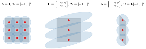
see proof in [6, Thm. 4.7]. By replacing the Lipschitz constant by the Lipschitz matrix fewer points are required cover the domain as illustrated in Fig. 1. The same can be seen in bounds for the covering number. [noheader=false]coverscalardata/fig_cover_scalar.dat [noheader=false]covermatrixdata/fig_cover_matrix.dat

Figure 1: Using the Lipschitz matrix instead of the Lipschitz constant reduces the number of $\epsilon$-balls required to cover a domain. For an $\epsilon=0.5$ cover, 9 points (dots) are required to cover a box (shaded quadrilateral) with $\epsilon$-balls (shaded ellipses) using the Lipschitz constant (left). In contrast, whereas only 3 points are required with the Lipschitz matrix (center, right). The center plot shows the perspective of the Lipschitz matrix altering the metric for the space; the right plot shows warping the domain to use the standard $\ell_{2}$ metric.

Theorem 2.1 ([36, Thm. 14.2]).

If ${\mathcal{D}}\subset\mathbb{R}^{m}$ is convex and ${\mathbf{L}}$ is full rank

(19) $$\left(\frac{1}{\epsilon}\right)^{m}\frac{\operatorname{{\mathrm{v}ol}}({\mathcal{D}})}{\operatorname{{\mathrm{v}ol}}({\mathcal{B}}_{1}(\cdot;{\mathbf{L}}))}\leq N_{\epsilon}({\mathcal{D}};{\mathbf{L}})\leq\left(\frac{3}{\epsilon}\right)^{m}\frac{\operatorname{{\mathrm{v}ol}}({\mathcal{D}})}{\operatorname{{\mathrm{v}ol}}({\mathcal{B}}_{1}(\cdot;{\mathbf{L}}))},$$

where $\operatorname{{\mathrm{v}ol}}$ denotes the Lebesgue measure in $\mathbb{R}^{m}$ and ${\mathcal{B}}_{1}(\cdot;{\mathbf{L}})$ the unit ball in $d_{{\mathbf{L}}}$.

This theorem implies $N_{\epsilon}({\mathcal{D}};{\mathbf{L}})=\mathcal{O}(\epsilon^{-m})$ when ${\mathbf{L}}$ is full rank. If ${\mathbf{L}}$ is low-rank we can apply this theorem by interpreting the Lipschitz matrix as warping the domain

(20) $${\mathbf{L}}{\mathcal{D}}\coloneqq\{{\mathbf{L}}{\mathbf{x}}:{\mathbf{x}}\in{\mathcal{D}}\}$$

and equipping this domain with the standard Euclidean metric $d({\mathbf{x}},{\mathbf{y}})=\|{\mathbf{x}}-{\mathbf{y}}\|_{2}$. Then covering number is

(21) $$N_{\epsilon}({\mathcal{D}};{\mathbf{L}})=N_{\epsilon}({\mathbf{L}}{\mathcal{D}};{\mathbf{I}}).$$

When ${\mathbf{L}}$ is rank-$r$, then ${\mathbf{L}}{\mathcal{D}}$ is an $r$-dimensional subset of $\mathbb{R}^{m}$. Applying Theorem 2.1 on this $r$-dimensional problem, note $N_{\epsilon}({\mathbf{L}}{\mathcal{D}};{\mathbf{I}})=\mathcal{O}(\epsilon^{-r})$.

In the remainder of this section we first establish a definition of uncertainty for Lipschitz functions and then use this definition to derive complexity results for approximation, integration, and optimization. Then we discuss how the Lipschitz matrix yields both asymptotic and non-asymptotic reductions to the complexity of these tasks when compared to the Lipschitz constant.

2.1 Uncertainty

One use of the Lipschitz matrix is to provide constraints on what values a function can take away from points where know its values. We denote these point queries consisting of a point ${\mathbf{x}}_{j}\in{\mathcal{D}}$ and a response $y_{j}\in\mathbb{R}$ by ${\mathcal{P}}_{M}=\{{\mathbf{x}}_{j},y_{j}\}_{j=1}^{M}$. This allows us to define the space of all Lipschitz functions with the Lipschitz matrix ${\mathbf{L}}$ that interpolate these point queries:

(22) $${\mathcal{L}}({\mathcal{D}},{\mathbf{L}},{\mathcal{P}}_{M})\coloneqq\{f\in{\mathcal{L}}({\mathcal{D}},{\mathbf{L}}):f({\mathbf{x}}_{j})=y_{j}\ \{{\mathbf{x}}_{j},y_{j}\}\in{\mathcal{P}}_{M}\}.$$

Using this notation we can then define the uncertainty set at a point ${\mathbf{x}}\in{\mathcal{D}}$

(23) $${\mathcal{U}}({\mathbf{x}};{\mathbf{L}},{\mathcal{P}}_{M})\coloneqq\{f({\mathbf{x}}):f\in{\mathcal{L}}({\mathcal{D}},{\mathbf{L}},{\mathcal{P}}_{M})\}.$$

This set is actually an interval for each ${\mathbf{x}}$. From the definition of Lipschitz matrix continuity Eq. 2, for any $f\in{\mathcal{L}}({\mathcal{D}},{\mathbf{L}},{\mathcal{P}}_{M})$ we have bounds

(24) $$y_{j}-\|{\mathbf{L}}({\mathbf{x}}-{\mathbf{x}}_{j})\|_{2}\leq f({\mathbf{x}})\leq y_{j}+\|{\mathbf{L}}({\mathbf{x}}-{\mathbf{x}}_{j})\|_{2}.$$

As these bounds apply for each $\{{\mathbf{x}}_{j}\}_{j=1}^{M}$ these provide lower and upper bounds for each point ${\mathbf{x}}$:

(25) $$f_{\min}({\mathbf{x}};{\mathbf{L}},{\mathcal{P}}_{M}) \coloneqq\max_{j=1,\ldots,M}y_{j}-\|{\mathbf{L}}({\mathbf{x}}-{\mathbf{x}}_{j})\|_{2},$$

(26) $$f_{\max}({\mathbf{x}};{\mathbf{L}},{\mathcal{P}}_{M}) \coloneqq\min_{j=1,\ldots,M}y_{j}+\|{\mathbf{L}}({\mathbf{x}}-{\mathbf{x}}_{j})\|_{2}.$$

Since these are the only constraints on $f({\mathbf{x}})$, the uncertainty set is an interval

(27) $${\mathcal{U}}({\mathbf{x}};{\mathbf{L}},{\mathcal{P}}_{M})=\left[f_{\min}({\mathbf{x}};{\mathbf{L}},{\mathcal{P}}_{M}),\ f_{\max}({\mathbf{x}};{\mathbf{L}},{\mathcal{P}}_{M})\right].$$

An important tool in our results is the central approximation

(28) $$f_{\mathrm{mid}}({\mathbf{x}};{\mathbf{L}},{\mathcal{P}}_{M})\coloneqq\frac{1}{2}\left(f_{\min}({\mathbf{x}})+f_{\max}({\mathbf{x}})\right).$$

This function minimizes the worst-case pointwise error of all Lipschitz approximations that interpolate the point set.

Lemma 2.2.

Given a domain ${\mathcal{D}}\subset\mathbb{R}^{m}$, Lipschitz matrix ${\mathbf{L}}\in\mathbb{R}^{m\times m}$, and point queries ${\mathcal{P}}_{M}=\{{\mathbf{x}}_{j},y_{j}\}_{j=1}^{M}$ then for any fixed $\widetilde{f}:{\mathcal{D}}\to\mathbb{R}$

(29) $$\sup_{f\in{\mathcal{L}}({\mathcal{D}},{\mathbf{L}},{\mathcal{P}}_{M})}|f({\mathbf{x}})-f_{\mathrm{mid}}({\mathbf{x}};{\mathbf{L}},{\mathcal{P}}_{M})|\leq\sup_{f\in{\mathcal{L}}({\mathcal{D}},{\mathbf{L}},{\mathcal{P}}_{M})}|f({\mathbf{x}})-\widetilde{f}({\mathbf{x}})|.$$

Proof 2.3.

This follows immediately from the uncertainty interval Eq. 27. Any other choice for $\widetilde{f}({\mathbf{x}})$ would have an error greater than $\frac{1}{2}[f_{\max}({\mathbf{x}})-f_{\min}({\mathbf{x}})]$ for some choice of $f$; cf., [34, pp. 12-13].

2.2 Complexity Results

The following results show the number of function queries are necessary to perform approximation, integration, and optimization to within a tolerance $\epsilon>0$ in the worst case depends on the $\epsilon$-covering of the domain.

2.2.1 Approximation

The following theorem shows that by querying a function at a minimax optimal design, the resulting central approximation yields the best approximation in the worst case.

Theorem 2.4.

Given a domain ${\mathcal{D}}\subset\mathbb{R}^{m}$ and a Lipschitz matrix ${\mathbf{L}}\in\mathbb{R}^{m\times m}$, the minimum number of point queries $M$ such that

(30) $$\sup_{f\in{\mathcal{L}}({\mathcal{D}},{\mathbf{L}})}\inf_{\widetilde{f}:{\mathcal{D}}\to\mathbb{R}}\max_{{\mathbf{x}}\in{\mathcal{D}}}|f({\mathbf{x}})-\widetilde{f}({\mathbf{x}})|\leq\epsilon\quad\text{where}\quad{\mathcal{P}}_{M}=\{{\mathbf{x}}_{j},f({\mathbf{x}}_{j})\}_{j=1}^{M}$$

is the $\epsilon$ internal covering number, $M=N_{\epsilon}({\mathcal{D}};{\mathbf{L}})$. The optimal point queries correspond to the $M$-point minimax optimal design, ${\mathcal{X}}({\mathcal{D}},M,{\mathbf{L}})$ and the optimal approximation $\widetilde{f}$ is the central approximation $f_{\mathrm{mid}}$.

Proof 2.5.

Using Lemma 2.2 we can remove the middle optimization in Eq. 30 by replacing $\widetilde{f}$ with the central approximation $f_{\mathrm{mid}}$:

(31) $$\sup_{f\in{\mathcal{L}}({\mathcal{D}},{\mathbf{L}})}\inf_{\widetilde{f}:{\mathcal{D}}\to\mathbb{R}}\max_{{\mathbf{x}}\in{\mathcal{D}}}|f({\mathbf{x}})-\widetilde{f}({\mathbf{x}})|=\sup_{f\in{\mathcal{L}}({\mathcal{D}},{\mathbf{L}})}\max_{{\mathbf{x}}\in{\mathcal{D}}}|f({\mathbf{x}})-f_{\mathrm{mid}}({\mathbf{x}};{\mathbf{L}},{\mathcal{P}}_{M})|.$$

The greatest uncertainty comes when $f({\mathbf{x}}_{j})=0$ for $j=1,\ldots,M$ and hence

(32) $$\sup_{f\in{\mathcal{L}}({\mathcal{D}},{\mathbf{L}})}\max_{{\mathbf{x}}\in{\mathcal{D}}}|f({\mathbf{x}})-f_{\mathrm{mid}}({\mathbf{x}};{\mathbf{L}},{\mathcal{P}}_{M})|=\max_{{\mathbf{x}}\in{\mathcal{D}}}\min_{j=1,\ldots,M}\|{\mathbf{L}}({\mathbf{x}}-{\mathbf{x}}_{j})\|_{2}.$$

Then the minimum $M$ to make the right hand side above less than $\epsilon$ is $N_{\epsilon}({\mathcal{D}},{\mathbf{L}})$ and the optimal queries correspond $N_{\epsilon}({\mathcal{D}},{\mathbf{L}})$-point minimax optimal design.

2.2.2 Optimization

The argument for the complexity of optimization is essentially that of approximation: unless we can approximate $f$ within $\epsilon$, we cannot globally optimize $f$ within $\epsilon$.

Theorem 2.6.

Suppose ${\mathcal{D}}\subset\mathbb{R}^{m}$ is compact and ${\mathbf{L}}\in\mathbb{R}^{m\times m}$. In the worst case, the minimum number of samples to find the maximum $f\in{\mathcal{L}}({\mathcal{D}},{\mathbf{L}})$ to within $\epsilon$ is the $\epsilon$-internal covering number $N_{\epsilon}({\mathbf{L}}{\mathcal{D}})$.

Proof 2.7.

As ${\mathcal{D}}$ is compact and $f$ is Lipschitz, $f$ must have a finite maximizer $f^{\star}$ where $f^{\star}=f({\mathbf{x}}^{\star})$ for at least one ${\mathbf{x}}^{\star}\in{\mathcal{D}}$. We first establish an upper bound on the number of point queries required. Using $M=N_{\epsilon}({\mathcal{D}},{\mathbf{L}})$ point queries ${\mathcal{P}}_{M}$ in a minimax optimal design there is a ${\mathbf{x}}_{j}$ in ${\mathcal{P}}_{M}$ such that $\|{\mathbf{L}}({\mathbf{x}}^{\star}-{\mathbf{x}}_{j})\|_{2}\leq\epsilon$. By Eq. 24

$$f({\mathbf{x}}^{\star})\leq f({\mathbf{x}}_{j})+\|{\mathbf{L}}({\mathbf{x}}-{\mathbf{x}}_{j})\|_{2}\leq f({\mathbf{x}}_{j})+\epsilon$$

and hence $f({\mathbf{x}}_{j})\geq f^{\star}-\epsilon$. To show this upper bound is obtained, consider the function $f\in{\mathcal{L}}({\mathcal{D}},{\mathbf{L}})$ where $f({\mathbf{x}})\geq 0$ for all ${\mathbf{x}}\in{\mathcal{D}}$, $f$ has optimizer $f({\mathbf{x}}^{\star})=2\epsilon=f^{\star}$, and $f$ has minimum integrand. If we choose $M<N_{\epsilon}({\mathcal{D}},{\mathbf{L}})$ point queries we can adversarially choose ${\mathbf{x}}^{\star}$ such that $\|{\mathbf{L}}({\mathbf{x}}-{\mathbf{x}}^{\star})\|_{2}>\epsilon$ and consequently $f({\mathbf{x}}_{j})<\epsilon$ for all $j=1,\ldots,M$.

2.2.3 Integration

This result parallels the one-dimensional Lipschitz case presented by Traub and Werschulz [34, chap. 2].

Theorem 2.8.

Suppose ${\mathcal{D}}\subset\mathbb{R}^{m}$ be compact and ${\mathbf{L}}\in\mathbb{R}^{m\times m}$. Let $\phi^{\star}$ denote the quadrature rule from integrating the central approximation on an $M$-point minimax optimal design

(33) $$\begin{split}&\phi^{\star}(f;M,{\mathbf{L}})\coloneqq\int_{{\mathbf{x}}\in{\mathcal{D}}}f_{\mathrm{mid}}({\mathbf{x}};{\mathbf{L}},{\mathcal{P}}_{M}){\,\mathrm{d}}{\mathbf{x}}\\ &\text{where}\quad{\mathcal{P}}_{M}=\{{\mathbf{x}}_{j},f({\mathbf{x}}_{j})\}_{j=1}^{M}\quad\text{and}\quad{\mathbf{x}}_{j}\in{\mathcal{X}}({\mathcal{D}},M,{\mathbf{L}}).\end{split}$$

Let $\phi$ denote any other $M$ point quadrature rule integrating an approximation $\widetilde{f}$, then

(34) $$\sup_{f\in{\mathcal{L}}({\mathcal{D}},{\mathbf{L}})}\left|\phi^{\star}(f)-\int_{{\mathbf{x}}\in{\mathcal{D}}}f({\mathbf{x}}){\,\mathrm{d}}{\mathbf{x}}\right|\leq\sup_{f\in{\mathcal{L}}({\mathcal{D}},{\mathbf{L}})}\left|\phi(f)-\int_{{\mathbf{x}}\in{\mathcal{D}}}f({\mathbf{x}}){\,\mathrm{d}}{\mathbf{x}}\right|.$$

Proof 2.9.

From Lemma 2.2, the central approximation has the smallest pointwise worst case error of any approximation interpolating the point queries ${\mathcal{P}}_{M}$. Thus

(35) $$\sup_{f\in{\mathcal{L}}({\mathcal{D}},{\mathbf{L}},{\mathcal{P}}_{M})}\left|\int_{{\mathbf{x}}\in{\mathcal{D}}}f_{\mathrm{mid}}({\mathbf{x}};{\mathbf{L}},{\mathcal{P}}_{M})-f({\mathbf{x}}){\,\mathrm{d}}{\mathbf{x}}\right|\leq\sup_{f\in{\mathcal{L}}({\mathcal{D}},{\mathbf{L}},{\mathcal{P}}_{M})}\left|\int_{{\mathbf{x}}\in{\mathcal{D}}}\widetilde{f}({\mathbf{x}})-f({\mathbf{x}}){\,\mathrm{d}}{\mathbf{x}}\right|.$$

Then as the points ${\mathcal{X}}({\mathcal{D}},M,{\mathbf{L}})$ minimize the worse case error in the central approximation, $\phi^{\star}$ is the worst-case optimal quadrature rule.

Corollary 2.10.

In the setting of Theorem 2.8,

(36) $$\left|\phi^{\star}(f;N_{\epsilon}({\mathcal{D}},{\mathbf{L}}),{\mathbf{L}})-\int_{{\mathbf{x}}\in{\mathcal{D}}}f({\mathbf{x}}){\,\mathrm{d}}{\mathbf{x}}\right|\leq\epsilon\cdot\operatorname{{\mathrm{v}ol}}({\mathcal{D}}).$$

Proof 2.11.

Let $M=N_{\epsilon}({\mathcal{D}},{\mathbf{L}})$. From the definition of $\phi^{\star}$ Eq. 33,

(37) $$\left|\phi^{\star}(f;M,{\mathbf{L}})-\int_{{\mathbf{x}}\in{\mathcal{D}}}f({\mathbf{x}}){\,\mathrm{d}}{\mathbf{x}}\right|\leq\int_{{\mathbf{x}}\in{\mathcal{D}}}|f_{\mathrm{mid}}({\mathbf{x}};{\mathbf{L}},{\mathcal{P}}_{M})-f({\mathbf{x}})|{\,\mathrm{d}}{\mathbf{x}}.$$

By Theorem 2.4, $|f_{\mathrm{mid}}({\mathbf{x}})-f({\mathbf{x}})|\leq\epsilon$; integrating this bound yields the result.

2.3 Asymptotic Improvements

The Lipschitz matrix provides two asymptotic improvements over the Lipschitz constant. If the Lipschitz matrix is rank-$r$, then complexity of approximation, integration, and optimization grows like $\mathcal{O}(\epsilon^{-r})$—not $\mathcal{O}(\epsilon^{-m})$. This also applies to ridge functions with ridge dimension $r$ by Theorem 1.1. Even if the Lipschitz matrix is full rank, the Lipschitz matrix can still substantially reduce the covering number compared to the Lipschitz constant. Interpreting the Lipschitz matrix as transforming the domain, from Theorem 2.1 we have the bound

(38) $$N_{\epsilon}({\mathcal{D}};{\mathbf{L}})=N_{\epsilon}({\mathbf{L}}{\mathcal{D}};{\mathbf{I}})\leq\frac{3^{m}}{\epsilon^{m}\operatorname{{\mathrm{v}ol}}({\mathcal{B}}_{1}(\cdot;{\mathbf{I}}))}\operatorname{{\mathrm{v}ol}}({\mathbf{L}}{\mathcal{D}}).$$

For the Lipschitz matrix and Lipschitz constant

(39) $$\operatorname{{\mathrm{v}ol}}({\mathbf{L}}{\mathcal{D}})=|\det{\mathbf{L}}|\cdot\operatorname{{\mathrm{v}ol}}({\mathcal{D}})\quad\text{and}\quad\operatorname{{\mathrm{v}ol}}(L{\mathcal{D}})=L^{m}\cdot\operatorname{{\mathrm{v}ol}}({\mathcal{D}}).$$

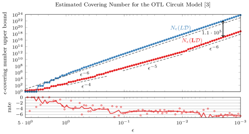
Hence if $|\det{\mathbf{L}}|\ll L^{m}$, we have substantially reduced the covering number. This is not uncommon: for the test problems shown in Table 1, $|\det{\mathbf{L}}|$ is multiple orders of magnitude smaller than $L^{m}$.

Table 1: Comparison of Lipschitz matrix, Lipschitz constant, and corresponding volumes for a variety of test functions [32] posed on the normalized domain ${\mathcal{D}}=[-1,1]^{m}$ with normalized outputs in $[0,1]$. Here we estimate ${\mathbf{L}}$ by minimizing the Frobenius norm using $1024$ gradient samples including the $2^{m}$ corners and otherwise sampled randomly.

test problem	dim.	$L$		$\sigma_{\text{max}}({\mathbf{L}})$		$\sigma_{\text{min}}({\mathbf{L}})$		$\operatorname{{\mathrm{v}ol}}(L{\mathcal{D}})$		$\operatorname{{\mathrm{v}ol}}({\mathbf{L}}{\mathcal{D}})$
Golinski volume [12]	$6$	$3$	$.0\cdot 10^{-1}$	$3$	$.0\cdot 10^{-1}$	$7$	$.3\cdot 10^{-4}$	$4$	$.3\cdot 10^{-2}$	$8$	$.4\cdot 10^{-9}$
OTL circult [3]	$6$	$5$	$.4\cdot 10^{-1}$	$5$	$.8\cdot 10^{-1}$	$1$	$.4\cdot 10^{-3}$	$1$	$.6\cdot 10^{0}$	$1$	$.4\cdot 10^{-5}$
piston [17]	$7$	$1$	$.0\cdot 10^{0}$	$1$	$.0\cdot 10^{0}$	$2$	$.6\cdot 10^{-3}$	$1$	$.3\cdot 10^{2}$	$2$	$.0\cdot 10^{-6}$
borehole [13]	$8$	$9$	$.0\cdot 10^{-1}$	$9$	$.2\cdot 10^{-1}$	$4$	$.6\cdot 10^{-6}$	$1$	$.1\cdot 10^{2}$	$5$	$.0\cdot 10^{-12}$
wing weight [10]	$10$	$3$	$.8\cdot 10^{-1}$	$4$	$.1\cdot 10^{-1}$	$4$	$.3\cdot 10^{-3}$	$5$	$.9\cdot 10^{-2}$	$2$	$.1\cdot 10^{-10}$

2.4 Non-asymptotic Improvement

Before the asymptotic limit, the Lipschitz matrix can slow the growth of covering number. Denoting the singular values of ${\mathbf{L}}$ in non-increasing order as $\sigma_{j}({\mathbf{L}})$, when $\epsilon\gg\sigma_{j}({\mathbf{L}})$ then ${\mathbf{L}}{\mathcal{D}}$ is effectively $j$-dimensional as a single $\epsilon$-ball can cover the dimensions $j+1,\ldots,m$. This temporally slows the growth of the covering number as illustrated in Fig. 2.

Figure 2: An upper bound on the covering number of the transformed domain. Here we estimate the covering number by counting the number of $\epsilon$-balls whose centers are on a grid with spacing $2\epsilon/\sqrt{m}$ that intersect the transformed domain; when the number of grid points exceeds $10^{4}$, random samples are used to estimate the number of $\epsilon$-balls intersecting the domain. The bottom plot shows the estimated growth rate of $N_{\epsilon}({\mathbf{L}}{\mathcal{D}})$ estimated using a finite difference (dots) and a 7-point median smoothed rate (line). The asymptotic separation of $1.1\cdot 10^{5}$ matches the ratio $\operatorname{{\mathrm{v}ol}}(L{\mathcal{D}})/\operatorname{{\mathrm{v}ol}}({\mathbf{L}}{\mathcal{D}})$.

3 Computing a Lipschitz Matrix

For a particular function $f$, our goal is to identify the smallest Lipschitz matrix ${\mathbf{L}}$ such that $f\in{\mathcal{L}}({\mathcal{D}},{\mathbf{L}})$. As discussed in Section 1.3, we must choose an ordering of positive semidefinite matrices. Here we minimize the Frobenius norm of the Lipschitz matrix yielding the program

(40) $$\begin{split}\min_{{\mathbf{L}}\in\mathbb{S}_{+}^{m\times m}}&\ \|{\mathbf{L}}\|_{\mathrm{F}}^{2}\\ \text{such that}&\ |f({\mathbf{x}}_{i})-f({\mathbf{x}}_{j})|\leq\|{\mathbf{L}}({\mathbf{x}}_{i}-{\mathbf{x}}_{j})\|_{2}\quad\forall{\mathbf{x}}_{i},{\mathbf{x}}_{j}\in{\mathcal{D}}.\end{split}$$

Ideally given $f$, we would identify this Frobenius-norm minimizing Lipschitz matrix in closed form. For most functions, this is infeasible. Instead, we approximate this program by discretizing the constraints using a finite number of point and/or gradient queries. This yields a semidefinite program to identify the Lipschitz matrix. Although tempting to enforce a low-rank constraint on the Lipschitz matrix in this program, we show this can yield in non-informative results. For the special case of quadratic functions, we provide a finite program exactly solving the full program Eq. 40. We finally illustrate how this discretized program converges with increasing queries.

3.1 Semidefinite Program for a Lipschitz Matrix

Both point queries ${\mathcal{P}}_{M}=\{{\mathbf{x}}_{j},f({\mathbf{x}}_{j})\}_{j=1}^{M}$ and gradient queries ${\mathcal{G}}_{N}=\{\nabla f({\mathbf{x}}_{k}^{\prime})\}_{k=1}^{N}$ provide constraints on the minimum Frobenius norm Lipschitz matrix. Recalling from Eq. 10 that the outer product of gradients is bounded above by ${\mathbf{L}}^{\top}{\mathbf{L}}$, the discretized minimum Frobenius-norm Lipschitz matrix solves

(41) $$\min_{{\mathbf{L}}\in\mathbb{S}_{+}^{m\times m}} \ \|{\mathbf{L}}\|_{\mathrm{F}}^{2}$$

such that $$|y_{i}-y_{j}|^{2} \leq\|{\mathbf{L}}({\mathbf{x}}_{i}-{\mathbf{x}}_{j})\|_{2}^{2}\quad \{{\mathbf{x}}_{i},y_{i}\},\{{\mathbf{x}}_{j},y_{j}\} \in{\mathcal{P}}_{M};$$

$${\mathbf{g}}_{k}{\mathbf{g}}_{k}^{\top} \preceq{\mathbf{L}}^{\top}{\mathbf{L}} {\mathbf{g}}_{k} \in{\mathcal{G}}_{N}.$$

This formulation has difficult non-convex quadratic constraints. Instead, we reformulate Eq. 41 in terms of the squared Lipschitz matrix ${\mathbf{H}}\coloneqq{\mathbf{L}}^{\top}{\mathbf{L}}$ and instead solve

(42) $$\min_{{\mathbf{H}}\in\mathbb{S}_{+}^{m\times m}} \ \operatorname{Tr}{\mathbf{H}}$$

such that $$|y_{i}-y_{j}|^{2} \leq({\mathbf{x}}_{i}-{\mathbf{x}}_{j})^{\top}{\mathbf{H}}({\mathbf{x}}_{i}-{\mathbf{x}}_{j}) \{{\mathbf{x}}_{i},y_{i}\},\{{\mathbf{x}}_{j},y_{j}\} \in{\mathcal{P}}_{M};$$

$${\mathbf{g}}_{k}{\mathbf{g}}_{k}^{\top} \preceq{\mathbf{H}} {\mathbf{g}}_{k} \in{\mathcal{G}}_{N}.$$

This, unlike Eq. 41, is convex semidefinite program. After parametrizing the space of symmetric matrices, this program has three sets of constraints: linear inequality constraints from the point queries, semidefinite constraints from the gradient queries, and the semidefinite constraint ${\mathbf{0}}\preceq{\mathbf{H}}$. Our numerical experiments use CVXOPT [1] to solve Eq. 42 and take ${\mathbf{L}}$ to be the symmetric positive definite square root of ${\mathbf{H}}$.

3.2 Semidefinite Program for an $\epsilon$-Lipschitz Matrix

We use a similar approach working in terms of the squared Lipschitz matrix ${\mathbf{H}}={\mathbf{L}}^{\top}{\mathbf{L}}$ to compute an $\epsilon$-Lipschitz matrix. However, because $\epsilon$-Lipschitz functions are not differentiable, gradient queries ${\mathcal{G}}_{N}$ do not constrain this matrix. This leaves only point queries which by Eq. 3 must satisfy

(43) $$|f({\mathbf{x}}_{1})-f({\mathbf{x}}_{2})|\leq\epsilon+\|{\mathbf{L}}({\mathbf{x}}_{1}-{\mathbf{x}}_{2})\|_{2}.$$

Replacing the point query constraint in Eq. 42 with this expression yields

(44) $$\min_{{\mathbf{H}}\in\mathbb{S}_{+}^{m\times m}} \ \operatorname{Tr}{\mathbf{H}}$$

such that $$\ \max(|y_{i}\!-\!y_{j}|\!-\!\epsilon,0)^{2}\leq\!({\mathbf{x}}_{i}-{\mathbf{x}}_{j})^{\!{\top}}{\mathbf{H}}({\mathbf{x}}_{i}-{\mathbf{x}}_{j})\ \ \{{\mathbf{x}}_{i},y_{i}\},\{{\mathbf{x}}_{j},y_{j}\}\!\in\!{\mathcal{P}}_{M}.\!\!\!$$

3.3 Low-rank Solutions

It is tempting to impose a rank constraint on ${\mathbf{H}}$, and consequently ${\mathbf{L}}$, to reduce complexity. Unfortunately, a low-rank constraint can yield misleading results. For example, suppose we have point queries $\{{\mathbf{x}}_{j},y_{j}\}_{j=1}^{M}={\mathcal{P}}_{M}$ where $\{{\mathbf{x}}_{j}\}_{j=1}^{M}$ is in general position. Then for almost every vector ${\mathbf{a}}\in\mathbb{R}^{m}$, the projections onto $\operatorname{Span}{\mathbf{a}}$ are distinct: ${\mathbf{a}}^{\top}{\mathbf{x}}_{i}\neq{\mathbf{a}}^{\top}{\mathbf{x}}_{j}$ for $i\neq j$. Thus, for almost every ${\mathbf{a}}$ there is a rank-1 Lipschitz matrix whose range is $\operatorname{Span}{\mathbf{a}}$:

(45) $${\mathbf{L}}_{{\mathbf{a}}}=\begin{bmatrix}{\mathbf{0}}\\ \alpha{\mathbf{a}}^{\top}\end{bmatrix}\in\mathbb{R}^{m\times m},\quad\alpha=\max_{i\neq j}\frac{|y_{i}-y_{j}|}{|{\mathbf{a}}^{\top}{\mathbf{x}}_{i}-{\mathbf{a}}^{\top}{\mathbf{x}}_{j}|}.$$

Hence regardless of the actual structure of $f$ we have likely mistakenly identified it as a one-dimensional ridge function. Gradient constraints for the Lipschitz matrix do not fail in a similar way. If $\operatorname{Range}\{\nabla f({\mathbf{x}}_{k}^{\prime})\}_{j=1}^{N}$ is $n$-dimensional, then ${\mathbf{H}}$, and consequently ${\mathbf{L}}$, must be at least rank-$n$.

3.4 Using the Determinant

In Section 2.3 we saw that the complexity of approximation, integration, and optimization are proportional to $|\det{\mathbf{L}}|$. Why not use the determinant as the objective function instead of the Frobenius norm in Eq. 40? There are two important reasons. We loose convexity: $\|{\mathbf{L}}\|_{\mathrm{F}}^{2}=\operatorname{Tr}{\mathbf{H}}$ is convex whereas $|\det{\mathbf{L}}|^{2}=\det{\mathbf{H}}$ is concave. The other is that the determinant yields uninformative Lipschitz matrices. As illustrated in the previous subsection, given finite point queries we can always find a low-rank Lipschitz matrix. As the determinant of this matrix is zero it is an optimal, but uninformative, Lipschitz matrix.

3.5 Quadratic Functions

In the case of a quadratic function we can show that there are only finite number of active gradient constraints of the continuous problem Eq. 40 yielding a finite semidefinite program for its Lipschitz matrix. Suppose $f$ is a quadratic function:

(46) $${\mathcal{D}}=[-1,1]^{m}\quad f:{\mathcal{D}}\to\mathbb{R}\quad\text{where}\quad f({\mathbf{x}})={\mathbf{x}}^{\top}{\mathbf{A}}{\mathbf{x}}+{\mathbf{b}}^{\top}{\mathbf{x}},$$

${\mathbf{A}}\in\mathbb{R}^{m\times m}$, and ${\mathbf{b}}\in\mathbb{R}^{m}$ whose gradient is $\nabla f({\mathbf{x}})=({\mathbf{A}}+{\mathbf{A}}^{\!{\top}}){\mathbf{x}}+{\mathbf{b}}$. The following theorem bounds the gradient outer-product above by points on the corners of the domain: those points where each coordinate takes on the value $-1$ or $1$.

Theorem 3.1.

Suppose $f:[-1,1]^{m}\to\mathbb{R}$ is a quadratic function as in Eq. 46. For any ${\mathbf{x}}\in{\mathcal{D}}$ there is a point ${\mathbf{c}}$ on a corner of ${\mathcal{D}}$ such that

(47) $$\nabla f({\mathbf{x}})\nabla f({\mathbf{x}})^{\top}\preceq\nabla f({\mathbf{c}})\nabla f({\mathbf{c}})^{\top}.$$

Proof 3.2.

Denote ${\mathbf{A}}_{S}={\mathbf{A}}+{\mathbf{A}}^{\top}$. Consider the difference of these two gradient outer-products for any ${\mathbf{c}}$ on the corner of ${\mathcal{D}}$ and ${\mathbf{x}}\in{\mathcal{D}}$:

(48) $$\nabla f({\mathbf{c}})\nabla f({\mathbf{c}})^{\top}-\nabla f({\mathbf{x}})\nabla f({\mathbf{x}})=\\ {\mathbf{A}}_{S}({\mathbf{c}}-{\mathbf{x}}){\mathbf{b}}^{\top}+{\mathbf{b}}({\mathbf{c}}-{\mathbf{x}})^{\top}{\mathbf{A}}_{S}+{\mathbf{A}}_{S}({\mathbf{c}}{\mathbf{c}}^{\top}-{\mathbf{x}}{\mathbf{x}}^{\top}){\mathbf{A}}_{S}.$$

As ${\mathbf{c}}$ is on the corner of $[-1,1]^{m}$, then ${\mathbf{c}}{\mathbf{c}}^{\top}\succeq{\mathbf{x}}{\mathbf{x}}^{\top}$ and

(49) $$\nabla f({\mathbf{c}})\nabla f({\mathbf{c}})^{\top}-\nabla f({\mathbf{x}})\nabla f({\mathbf{x}})\succeq{\mathbf{A}}_{S}({\mathbf{c}}-{\mathbf{x}}){\mathbf{b}}^{\top}+{\mathbf{b}}({\mathbf{c}}-{\mathbf{x}})^{\top}{\mathbf{A}}_{S}.$$

As ${\mathbf{c}}$ is on a corner, there is a ${\mathbf{c}}$ such that the entires of the entries of ${\mathbf{c}}-{\mathbf{x}}$ can have any combination of signs $\{+,0\}$ or $\{-,0\}$. Thus we can choose a corner such that ${\mathbf{A}}_{S}({\mathbf{c}}-{\mathbf{x}}){\mathbf{b}}^{\top}$ has nonnegative entries. Then the right hand side above is nonnegative and we conclude

(50) $$\nabla f({\mathbf{c}})\nabla f({\mathbf{c}})^{\top}-\nabla f({\mathbf{x}})\nabla f({\mathbf{x}})\succeq{\mathbf{0}}.$$

As a result of this theorem, the Frobenius-norm minimizing Lipschitz matrix for a quadratic function is the solution to a finite-dimensional semidefinite program

(51) $$\operatorname*{argmin}_{{\mathbf{H}}\in\mathbb{S}_{+}^{m\times m}} \ \operatorname{Tr}{\mathbf{H}}$$

such that $$\ {\mathbf{g}}_{k}{\mathbf{g}}_{k}^{\top}\preceq{\mathbf{H}}\qquad{\mathbf{g}}_{k}\in\{\nabla f({\mathbf{c}}_{k})\}_{k=1}^{2^{m}}$$

where $\{{\mathbf{c}}_{k}\}_{k=1}^{2^{m}}$ are the $2^{m}$ corners of ${\mathcal{D}}=[-1,1]^{m}$.

3.6 Convergence in Queries

With increasing point and gradient queries, the solution the finite-constraint semidefinite program Eq. 41 converges to the continuous-constraint program Eq. 40 if the function $f$ is Lipschitz. Let ${\mathbf{H}}_{M,N}$ denote the solution to Eq. 42 with ${\mathcal{P}}_{M}$ and ${\mathcal{G}}_{N}$. If ${\mathcal{P}}_{M}\subset{\mathcal{P}}_{M+1}$ and ${\mathcal{G}}_{N}\subset{\mathcal{G}}_{N+1}$ then $\operatorname{Tr}{\mathbf{H}}_{M,N}\leq\operatorname{Tr}{\mathbf{H}}_{M+1,N}$ and $\operatorname{Tr}{\mathbf{H}}_{M,N}\leq\operatorname{Tr}{\mathbf{H}}_{M,N+1}$. As $f$ is Lipschitz there exists a solution ${\mathbf{H}}$ to the continuous-constraint problem and $\operatorname{Tr}{\mathbf{H}}_{M,N}\leq\operatorname{Tr}{\mathbf{H}}$. Then as $\operatorname{Tr}{\mathbf{H}}_{M,N}\to\operatorname{Tr}{\mathbf{H}}$, ${\mathbf{H}}_{M,N}\to{\mathbf{H}}$.

3.7 Convergence Rate

An important practical question is how fast do finite query approximations converge to the continuous-constraint Lipschitz matrix Eq. 40? Unfortunately if we use random sampling this rate can be very slow. Figure 3 shows a quadratic approximation to the OTL Circuit function. As this is a quadratic function, we know the Lipschitz matrix is determined by the gradient at the corners. The probability of querying within $\epsilon$ of these points when sampling randomly is $\mathcal{O}(\epsilon^{-m})$; hence convergence with gradient queries is $\mathcal{O}(\epsilon^{-m})$ and convergence with point queries is $\mathcal{O}(\epsilon^{-2m})$. This is very slow! However, this slow convergence is not surprising as the Lipschitz matrix tracks the maximum rate of change.

Figure 3: The convergence of a discrete estimate of the Frobenius norm minimizing squared Lipschitz matrix ${\mathbf{H}}$ to it true value ${{\widehat{{\mathbf{H}}}}}$ for a least squares quadratic approximation to the 6-parameter OTL circuit function on a $8^{6}$ point grid. Finite difference gradients are forward differences in each unit direction from one central point requiring seven function evaluations. For each number of queries $M$ and $N$ we randomly sample the domain with uniform probability. One hundred repetitions are performed, with the median shown by a solid line and the shaded region enclosing the $25$th to $75$th percentile. The top plot shows the error in the squared Lipschitz matrix while the bottom plot shows the wall clock time on a Xeon E5-2620 clocked at 2.1 GHz using OpenBLAS with one thread and CVXOPT 1.2.5.

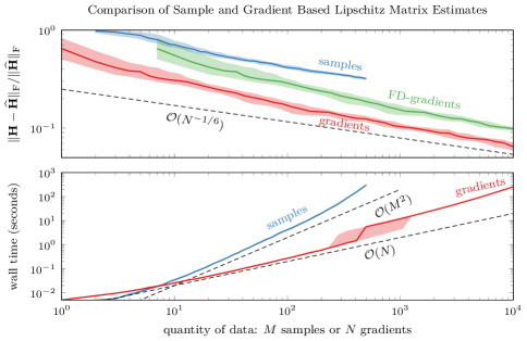
Although this result is distressing, hope is not lost. Many problems in science and engineering are approximately monotonic over their domains. Hence we can employ a similar argument to Theorem 3.1 to justify that querying gradients at the corners of the domain yields an accurate approximation of the Lipschitz matrix. We employ this strategy throughout the remainder of this manuscript to estimate the Lipschitz matrix, potentially in combination with other random point or gradient queries.

4 Ridge Approximation Error Bound

In the introduction, Theorem 1.1 showed that functions with low-rank Lipschitz matrices ridge functions. Here we provide a related result that bounds the error made when approximating Lipschitz function by a ridge function. This result is analogous to the error bound associated with the MeGO matrix [4, Thm. 4.3].

Theorem 4.1.

Suppose $f\in{\mathcal{L}}({\mathcal{D}},{\mathbf{L}})$, $\widetilde{f}\in{\mathcal{L}}({\mathcal{D}},{\mathbf{L}}{\mathbf{U}}{\mathbf{U}}^{\top})$ where ${\mathbf{U}}\in\mathbb{R}^{m\times n}$ and ${\mathbf{U}}^{\top}{\mathbf{U}}={\mathbf{I}}$, and $\{{\mathbf{x}}_{j}\}_{j=1}^{M}\subset{\mathcal{D}}$, then

(52) $$\max_{{\mathbf{x}}\in{\mathcal{D}}}|f({\mathbf{x}})-\widetilde{f}({\mathbf{x}})|\leq\max_{j=1,\ldots,M}|f({\mathbf{x}}_{j})-\widetilde{f}({\mathbf{x}}_{j})|+\\ 2\max_{{\mathbf{x}}\in{\mathcal{D}}}\min_{j=1,\ldots,M}\|{\mathbf{L}}{\mathbf{U}}{\mathbf{U}}^{\top}({\mathbf{x}}_{j}-{\mathbf{x}})\|_{2}+\sigma_{\max}({\mathbf{L}}({\mathbf{I}}-{\mathbf{U}}{\mathbf{U}}^{\top}))\cdot\operatorname{diam}({\mathcal{D}})$$

where $\sigma_{\max}({\mathbf{A}})$ denotes the largest singular value of ${\mathbf{A}}$ and $\operatorname{diam}({\mathcal{D}})$ denotes the diameter of the set ${\mathcal{D}}$; $\operatorname{diam}({\mathcal{D}})\coloneqq\max_{{\mathbf{x}}_{1},{\mathbf{x}}_{2}\in{\mathcal{D}}}\|{\mathbf{x}}_{1}-{\mathbf{x}}_{2}\|_{2}$.

Proof 4.2.

Suppose ${\mathbf{x}}\in{\mathcal{D}}$ is fixed. Let $j=\operatorname*{argmin}_{k}\|{\mathbf{L}}{\mathbf{U}}{\mathbf{U}}^{\top}({\mathbf{x}}_{k}-{\mathbf{x}})\|_{2}$ and define $\epsilon\coloneqq\max_{j=1,\ldots,M}|f({\mathbf{x}}_{j})-\widetilde{f}({\mathbf{x}}_{j})|$. Inserting an additive identity,

(53) $$|f({\mathbf{x}})\!-\!\widetilde{f}({\mathbf{x}})| =|f({\mathbf{x}})-\widetilde{f}({\mathbf{x}})+[f({\mathbf{x}}_{j})-\widetilde{f}({\mathbf{x}}_{j})]-[f({\mathbf{x}}_{j})-\widetilde{f}({\mathbf{x}}_{j})]|$$

(54) $$\leq|f({\mathbf{x}})-f({\mathbf{x}}_{j})|+|\widetilde{f}({\mathbf{x}})-\widetilde{f}({\mathbf{x}}_{j})|+\epsilon.$$

Invoking each function’s Lipschitz matrix and again inserting the identify,

(55) $$|f({\mathbf{x}})\!-\!\widetilde{f}({\mathbf{x}})| \leq\|{\mathbf{L}}({\mathbf{x}}-{\mathbf{x}}_{j})\|_{2}+\|{\mathbf{L}}{\mathbf{U}}{\mathbf{U}}^{\top}({\mathbf{x}}-{\mathbf{x}}_{j})\|_{2}+\epsilon$$

(56) $$\leq\|{\mathbf{L}}({\mathbf{U}}{\mathbf{U}}^{\top}\!+{\mathbf{I}}-{\mathbf{U}}{\mathbf{U}}^{\top})({\mathbf{x}}-{\mathbf{x}}_{j})\|_{2}+\|{\mathbf{L}}({\mathbf{U}}{\mathbf{U}}^{\top})({\mathbf{x}}-{\mathbf{x}}_{j})\|_{2}+\epsilon.$$

Finally, using the triangle inequality in the last term,

(57) $$|f({\mathbf{x}})\!-\!\widetilde{f}({\mathbf{x}})| \leq 2\|{\mathbf{L}}{\mathbf{U}}{\mathbf{U}}^{\top}({\mathbf{x}}-{\mathbf{x}}_{j})\|_{2}+\|{\mathbf{L}}({\mathbf{I}}-{\mathbf{U}}{\mathbf{U}}^{\top})({\mathbf{x}}-{\mathbf{x}}_{j})\|_{2}+\epsilon.$$

Then defining $\delta\coloneqq\max_{{\mathbf{x}}\in{\mathcal{D}}}\min_{j=1,\ldots,M}\|{\mathbf{L}}{\mathbf{U}}{\mathbf{U}}^{\top}({\mathbf{x}}-{\mathbf{x}}_{j})\|_{2}$ and bounding the second term by the diameter, we obtain a result independent of ${\mathbf{x}}$

(58) $$|f({\mathbf{x}})-\widetilde{f}({\mathbf{x}})| \leq\epsilon+2\delta+\sigma_{\max}({\mathbf{L}}({\mathbf{I}}-{\mathbf{U}}{\mathbf{U}}^{\top}))\cdot\operatorname{diam}({\mathcal{D}}).$$

We can then use this theorem to motivate a particular choice for ${\mathbf{U}}$ and function evaluations ${\mathbf{x}}_{j}$. First note that each term in this theorem has an important interpretation:

$$\max_{j}|f({\mathbf{x}}_{j})-\widetilde{f}({\mathbf{x}}_{j})| \{{\mathbf{x}}_{j}\}_{j=1}^{M}$$ function approximation error on ,

$$\max_{{\mathbf{x}}\in{\mathcal{D}}}\min_{j}\|{\mathbf{L}}{\mathbf{U}}{\mathbf{U}}^{\top}({\mathbf{x}}_{j}-{\mathbf{x}})\|_{2} \{{\mathbf{x}}_{j}\}_{j=1}^{M} {\mathcal{D}}$$ dispersion of in ,

$$\sigma_{\max}({\mathbf{L}}({\mathbf{I}}-{\mathbf{U}}{\mathbf{U}}^{\top})) \text{ \emph{Lipschitz matrix approximation error}}.$$

To minimize the Lipschitz matrix approximation error we should choose the leading eigenvectors of ${\mathbf{L}}$ as the columns of ${\mathbf{U}}$ (or right singular vectors of ${\mathbf{L}}$ is not symmetric positive definite). With ${\mathbf{U}}$ selected, we can minimize dispersion by constructing a minimax design of experiments ${\mathcal{X}}({\mathcal{D}},M,{\mathbf{L}}{\mathbf{U}}{\mathbf{U}}^{\top})$ as in Eq. 18. As discussed in Section 2.1, the number of function evaluations required to obtain a particular dispersion (the covering number) no longer grows with the dimension of the domain, but instead the rank of the Lipschitz matrix ${\mathbf{L}}{\mathbf{U}}{\mathbf{U}}^{\top}$. If $f$ is a ridge function then we can make the function approximation error zero; otherwise, this is not the case. If two coordinates have the same projection, ${\mathbf{U}}^{\top}{\mathbf{x}}_{i}={\mathbf{U}}^{\top}{\mathbf{x}}_{j}$, and $f({\mathbf{x}}_{i})\neq f({\mathbf{x}}_{j})$, then the function approximation error is at least $|f({\mathbf{x}}_{i})-f({\mathbf{x}}_{j})|/2$.

Before concluding, we note two corollaries when the function approximation error is zero.

Corollary 4.3.

In the setting of Theorem 4.1, let ${\mathbf{U}}$ be the identity matrix and choose $\widetilde{f}$ such that $f({\mathbf{x}}_{j})=\widetilde{f}({\mathbf{x}}_{j})$, then

(59) $$\max_{{\mathbf{x}}\in{\mathcal{D}}}|f({\mathbf{x}})-\widetilde{f}({\mathbf{x}})|\leq 2\max_{{\mathbf{x}}\in{\mathcal{D}}}\min_{j=1,\ldots,M}\|{\mathbf{L}}({\mathbf{x}}_{j}-{\mathbf{x}})\|_{2}.$$

Corollary 4.4.

In the setting of Theorem 4.1, let $f$ be a ridge function and ${\mathbf{U}}$ be a basis for the range of ${\mathbf{L}}$. Taking $\widetilde{f}$ such that $f({\mathbf{x}}_{j})=\widetilde{f}({\mathbf{x}}_{j})$, then

(60) $$\max_{{\mathbf{x}}\in{\mathcal{D}}}|f({\mathbf{x}})-\widetilde{f}({\mathbf{x}})|\leq 2\max_{{\mathbf{x}}\in{\mathcal{D}}}\min_{j=1,\ldots,M}\|{\mathbf{L}}{\mathbf{U}}{\mathbf{U}}^{\top}({\mathbf{x}}_{j}-{\mathbf{x}})\|_{2}.$$

5 Design of Experiments

Given a particular function, where should we evaluate it to provide the most information? This is the subject of the design of computer experiments [28], a subfield of experimental design (see, e.g., [9]) distinguished by the assumption that observations are deterministic; e.g., $f({\mathbf{x}})$ returns only one value. From the ridge approximation error bound in Theorem 4.1 and the earlier complexity results in Section 2.2, a good experimental design of points $\{{\mathbf{x}}_{j}\}_{j=1}^{M}\subset{\mathcal{D}}$ should minimize the dispersion in the Lipschitz matrix metric:

(61) $$\delta(\{{\mathbf{x}}_{j}\}_{j=1}^{M},{\mathcal{D}},{\mathbf{L}})\coloneqq\max_{{\mathbf{x}}\in{\mathcal{D}}}\min_{j=1,\ldots,M}\|{\mathbf{L}}({\mathbf{x}}-{\mathbf{x}}_{j})\|_{2}.$$

Minimizing the dispersion yields in a minimax optimal design; cf. Eq. 18:

(62) $${\mathcal{X}}({\mathcal{D}},M,{\mathbf{L}})=\operatorname*{argmin}_{\{{\mathbf{x}}_{j}\}_{j=1}^{M}\subset{\mathcal{D}}}\max_{{\mathbf{x}}\in{\mathcal{D}}}\min_{j=1,\ldots,M}\|{\mathbf{L}}({\mathbf{x}}-{\mathbf{x}}_{j})\|_{2}.$$

There is a substantial body of literature on solving this problem; see, e.g., [24] for a recent review. Here we provide a motivating example illustrating why an minimax design in the Lipschitz metric is important. Then we provide a brief description of how we construct locally optimal low-dispersion designs and illustrate the performance of this algorithm.

5.1 A Motivating Example

Consider a ridge function

(63) $$f:[-1,1]^{10}\to\mathbb{R},\qquad f({\mathbf{x}})=\sin({\mathbf{1}}^{\top}{\mathbf{x}})$$

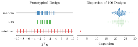
with a one-dimensional active subspace $\operatorname{Span}\{{\mathbf{1}}\}$ and a rank-one Lipschitz matrix ${\mathbf{L}}={\mathbf{1}}{\mathbf{1}}^{\top}$. If we randomly select points $\{{\mathbf{x}}_{j}\}_{j=1}^{M}$ with uniform probability over the domain, their sum tends to concentrate around the mean (zero) when projected onto the active subspace as seen in Fig. 4. The same is true with a Latin hypercube design where points are randomly selected so that projection onto the coordinate axes results in evenly spaced points. However, this is not true when we construct a minimax design under the Lipschitz matrix metric. This design has much lower dispersion and consequently we can construct much more accurate approximations according to Theorem 4.1.

Figure 4: In high dimensional spaces it is critical to incorporate structure to construct good experimental designs. In this example we consider ridge function Eq. 63 and measure the quality of uniform random sampling and Latin hypercube sampling (LHS) in the Lipschitz matrix metric.

5.2 Constructing Minimax Designs

Finding even an approximately optimal minimax design is challenging: it requires solving a deeply nested optimization problem Eq. 62 in a high dimensional space with many local minimizers with large dispersion. Here we briefly describe a combination of three algorithms that we use to construct the minimax designs appearing in the remainder of this paper. Each algorithm primarily uses bounded Voronoi vertices under the Lipschitz matrix metric. All such vertices can be computed using Qhull [2] or a random subset by sequential projection [19]; using sequential projection allows us to employ this combination algorithms spaces of moderate dimension, i.e., $m>4$.

To avoid finding a local minimizer with a large dispersion, the first two algorithm construct a good initial design that is then refined to local optimality. First, we construct a maximin coffeehouse design [21] where we greedily add new points to the design maximizing their distance from existing points in the design

(64) $${\mathbf{x}}_{k}\leftarrow\operatorname*{argmax}_{{\mathbf{x}}\in{\mathcal{D}}}\min_{j=1,\ldots,k-1}\|{\mathbf{L}}({\mathbf{x}}-{\mathbf{x}}_{j})\|_{2}.$$

This optimizer ${\mathbf{x}}_{k}$ is a bounded Voronoi vertex that we can (approximately) identify by a finite minimization over (a subset of) these vertices. Second, we perform a few iterations of block coordinate descent [30] to maximize the minimum pairwise distance

(65) $${\mathbf{x}}_{k}^{\ell+1}\leftarrow\operatorname*{argmax}_{{\mathbf{x}}\in{\mathcal{D}}}\min_{\begin{subarray}{c}j=1,\ldots,M\\ j\neq k\end{subarray}}\|{\mathbf{L}}({\mathbf{x}}-{\mathbf{x}}_{j}^{\ell})\|_{2}$$

Again, we can (approximately) solve this optimization problem by a finite minimization over (a subset of) the bounded Voronoi vertices. Finally this design initializes a variant of Lloyd’s algorithm to find a locally optimal minimax design [33]. At each iteration we identify the bounded Voronoi vertices ${\mathbf{v}}_{i}^{\ell}$ associated with the design $\{{\mathbf{x}}_{j}^{\ell}\}_{j=1}^{M}$ and then move ${\mathbf{x}}_{j}^{\ell}$ to be the circumcenters of its Voronoi cell

(66) $${\mathbf{x}}_{k}^{\ell+1}\leftarrow\operatorname*{argmin}_{{\mathbf{x}}\in{\mathcal{D}}}\max_{{\mathbf{v}}_{i}^{\ell}\in\text{Voronoi cell of }{\mathbf{x}}_{k}^{\ell}}\|{\mathbf{L}}({\mathbf{x}}-{\mathbf{v}}_{i}^{\ell})\|_{2}.$$

If this iteration converges, the design satisfies the local optimality conditions for a minimax design [6, Thm. 4.7]. Note that if the Lipschitz matrix is low-rank (i.e., rank one, two, or three) it feasible to compute all the bounded Voronoi vertices even if the ambient space is high dimensional.

Figure 5: The dispersion of several types of designs for the OTL circuit function using twenty trials. The solid line shows the median and the shaded regions the 25th to 75th percentile.

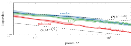
It is tempting to think that a minimax design is only necessary when function evaluations are costly. However, as Fig. 5 illustrates increasing the number of random and Latin hypercube samples decreases dispersion only very slowly at $\mathcal{O}(M^{-1/6})$ whereas we see the minimax design temporally converges faster and has a substantially reduced dispersion (see discussion in subsections 2.3 and 2.4). Hence if we seek a low-dispersion design for accurate approximation, integration, or optimization it is critical to construct an approximate minimax design.

6 Parameter Reduction

Using the Lipschitz matrix, we can perform dimension reduction by constructing a ridge approximation

(67) $$f({\mathbf{x}})\approx\widetilde{f}({\mathbf{x}})\coloneqq g({\mathbf{U}}^{\top}{\mathbf{x}}),\quad g:\mathbb{R}^{n}\to\mathbb{R},\quad{\mathbf{U}}\in\mathbb{R}^{m\times n}.$$

Since $g$ is a ridge function, $g$ has at most a rank-$n$ Lipschitz matrix (Theorem 1.1) and complexity of tasks now scales with the ridge dimension $n$ and no longer the dimension of the ambient space $m$. There are many ways to construct ridge approximations; e.g., picking ${\mathbf{U}}$ from the dominant eigenvectors of the MeGO matrix and then fitting a polynomial [4] or directly picking ${\mathbf{U}}$ and polynomial $g$ via optimization [5, 14]. Here we construct a ridge approximation using the Lipschitz matrix in light of Theorem 4.1.

6.1 Building a Ridge Approximation

Our choice of the ridge subspace is clear from Theorem 4.1: the leading $n$ eigenvectors of the Lipschitz matrix form ${\mathbf{U}}\in\mathbb{R}^{m\times n}$, same as when using the MeGO matrix. To construct a ridge approximation satisfying Theorem 4.1 we need to choose a ridge function $\widetilde{f}\in{\mathcal{L}}({\mathcal{D}},{\mathbf{L}}{\mathbf{U}}{\mathbf{U}}^{\top})$. Due to the constraints its Lipschitz matrix, $\widetilde{f}$ may not interpolate point queries; i.e., $\widetilde{f}({\mathbf{x}}_{j})\neq f({\mathbf{x}}_{j})$. Hence to a compatible ridge approximation $\widetilde{f}$ we first solve an optimization problem for function values $\widetilde{y}_{j}=\widetilde{f}({\mathbf{x}}_{j})$ minimizing the $\ell_{1}$ error (or equivalently any other convex norm)

(68) $$\widetilde{{\mathbf{y}}}=\operatorname*{argmin}_{{\mathbf{y}}\in\mathbb{R}^{M}}\sum_{j=1}^{M}|y_{j}-f({\mathbf{x}}_{j})|,\quad\text{such that}\quad|y_{j}-y_{k}|\leq\|{\mathbf{L}}{\mathbf{U}}{\mathbf{U}}^{\top}({\mathbf{x}}_{j}-{\mathbf{x}}_{k})\|_{2}.$$

Then these function values define point queries $\widetilde{\mathcal{P}}_{M}=\{{\mathbf{x}}_{j},\widetilde{y}_{j}\}_{j=1}^{M}$ and define $\widetilde{f}$ to be the central approximation of this data, cf. Eq. 28:

(69) $$\widetilde{f}({\mathbf{x}})=\frac{1}{2}\left[f_{\min}({\mathbf{x}};{\mathbf{L}}{\mathbf{U}}{\mathbf{U}}^{\top},\widetilde{\mathcal{P}}_{M})+f_{\max}({\mathbf{x}};{\mathbf{L}}{\mathbf{U}}{\mathbf{U}}^{\top},\widetilde{\mathcal{P}}_{M})\right].$$

As $\widetilde{f}$ approximates $f$ with a maximum error $\epsilon=\max_{j}|y_{j}-f({\mathbf{x}}_{j})|$, the uncertainty associated with $\widetilde{f}$ is, cf. Eq. 27,

(70) $${\mathcal{U}}_{\epsilon}({\mathbf{x}};{\mathbf{L}}{\mathbf{U}}{\mathbf{U}}^{\top},\widetilde{\mathcal{P}}_{M})=[f_{\min}({\mathbf{x}};{\mathbf{L}}{\mathbf{U}}{\mathbf{U}}^{\top},\widetilde{\mathcal{P}}_{M})-\epsilon\ ,\ f_{\max}({\mathbf{x}};{\mathbf{L}}{\mathbf{U}}{\mathbf{U}}^{\top},\widetilde{\mathcal{P}}_{M})+\epsilon].$$

6.2 Typical Workflow

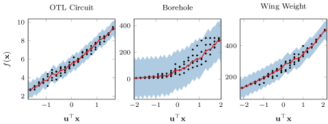
A typical workflow for using the Lipschitz matrix for dimension reduction starts with querying the gradient on the corners of the domain and using this data to estimate the Lipschitz matrix. Then, picking the active subspace to be the span of the leading eigenvector ${\mathbf{U}}\in\mathbb{R}^{m\times 1}$ of ${\mathbf{L}}$, we construct a 20-point minimax design under this metric ${\mathbf{L}}{\mathbf{U}}{\mathbf{U}}^{\top}$, $\{{\mathbf{x}}_{j}\}_{j=1}^{20}$. To better estimate the variability at each point, we take 5 maximin coffeehouse samples on each domain ${\mathcal{D}}_{j}=\{{\mathbf{x}}\in{\mathcal{D}}:{\mathbf{U}}^{\top}{\mathbf{x}}={\mathbf{U}}^{\top}{\mathbf{x}}_{j}\}$ in the Lipschitz metric ${\mathbf{L}}$. Finally, we construct the ridge approximation as described in the previous section. Figure 6 shows three examples of this workflow and the associated uncertainty.

Figure 6: Three ridge approximations as described in Section 6.2. In each plot the $x$-coordinate shows the projection of the domain onto the one-dimensional active subspace. The red curve denotes the central approximation, the black dots the data used to construct the approximation, and the shaded region the uncertainty.

7 Uncertainty Quantification

When working with expensive deterministic computer simulations it is often necessary to employ an approximation of certain quantities of interest, called a response surface or a surrogate. Supposing we have constructed this approximation using samples of $f$, it is natural ask: what are the range of possible values our approximation could take away from these samples? This is often called uncertainty in this setting. Gaussian processes provide one approach to define an uncertainty [25, sec. 2.2] and the Lipschitz constant provides another [26]. These two techniques are based on different assumptions and yield different results as illustrated in Fig. 7. The Gaussian process approach assumes that $f$ is a Gaussian process conditioned on the measurements $y_{j}=f({\mathbf{x}}_{j})$, maximizes the likelihood of a parameterized covariance kernel based on observations, and then computes the probability of observing $f({\mathbf{x}})$; the uncertainty is visualized as all function values above some probability threshold. In contrast, the Lipschitz approach assumes measurements $y_{j}=f({\mathbf{x}}_{j})$ comes from a Lipschitz function, chooses the smallest Lipschitz constant that consistent with this data, and defines uncertainty as the range of possible function values consistent with this Lipschitz constant and data; namely, the uncertainty set ${\mathcal{U}}$ Eq. 23. Replacing the Lipschitz constant by the Lipschitz matrix allows us to reduce uncertainty.

Figure 7: A comparison of Gaussian Process and the Lipschitz notions of uncertainty. Here we use ten samples of $f(x)=\sin(3\pi x)$ on ${\mathcal{D}}=[-1,1]$ denoted by dots, with $f$ shown by the black line. In both plots, the shaded area denotes the uncertainty estimate. The left plot shows the Gaussian process with zero-mean $m({\mathbf{x}})=0$ and squared exponential covariance $k({\mathbf{x}},{\mathbf{x}}^{\prime})=\exp(-\frac{1}{2}\|\ell({\mathbf{x}}-{\mathbf{x}}^{\prime})\|_{2}^{2})$ where $\ell=0.157$ has been chosen to maximize the marginal likelihood [25, subsec. 2.7.1]; the probability threshold $\delta$ corresponds to one-standard deviation. The right plot shows the Lipschitz uncertainty with Lipschitz constant $L=8.39$ estimated from the samples.

7.1 Decreasing Uncertainty

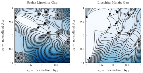
As the Lipschitz matrix more accurately encodes variability in the function, it can reduces uncertainty compared to the scalar Lipschitz constant. Figure 8 illustrates the improvement of the Lipschitz matrix over the Lipschitz constant on a two dimensional example. Table 2 demonstrates the same reduction in uncertainty occurs in higher dimensional examples. This example shows that uncertainty is reduced the most when Lipschitz matrix is used both when constructing the minimax design and evaluating the uncertainty set.

Figure 8: A plot of the gap between the upper and lower Lipschitz bounds. Here we use function values taken the OTL circuit test problem using the first two parameters, holding the remainder at their central values; additionally the domain has been normalized to $[-1,1]^{2}$. In each plot, the contours show an increase of $0.1$ in the gap. Here the uncertainty set, the Lipschitz constant, and Lipschitz matrix were all estimated using the ten samples marked with dots. Here $L=2.38$ and ${\mathbf{L}}=\begin{bmatrix}1.6&0\\ -1.3&1.6\end{bmatrix}$.

Table 2: Estimated maximum pointwise uncertainty over the domain using a 100-point minimax design with either isotropic or Lipschitz matrix metric. The maximum uncertainty is computed by extensively sampling the domain and measuring the diameter the Lipschitz constant or Lipschitz matrix uncertainty set. To aid comparison, each function’s range has been normalized to $[0,1]$.

test problem	dim.	isotropic Lip. const. uncertainty		isotropic Lip. matrix uncertainty		Lipschitz Lip. matrix uncertainty		ratio
Golinski volume [12]	$6$	$0$	$.69$	$0$	$.42$	$0$	$.15$	$4$	$.72$
OTL circult [3]	$6$	$1$	$.32$	$0$	$.61$	$0$	$.44$	$3$	$.01$
piston [17]	$7$	$3$	$.04$	$1$	$.26$	$0$	$.62$	$4$	$.90$
borehole [13]	$8$	$3$	$.12$	$1$	$.20$	$0$	$.49$	$6$	$.35$
wing weight [10]	$10$	$1$	$.72$	$0$	$.82$	$0$	$.39$	$4$	$.41$

7.2 Visualizing Uncertainty on Shadow Plots

Shadow plots are an important tool for visualizing functions with a high-dimensional domain. To include the uncertainty in shadow plots, we generalize the uncertainty set Eq. 23 to take set-valued inputs

(71) $$\begin{split}{\mathcal{U}}({\mathcal{S}};{\mathbf{L}},{\mathcal{P}}_{M})&\coloneqq\bigcup_{{\mathbf{x}}\in{\mathcal{S}}}{\mathcal{U}}({\mathbf{x}};{\mathbf{L}},{\mathcal{P}}_{M})\\ &=\left[\min_{{\mathbf{x}}\in{\mathcal{S}}}\max_{j}y_{j}-\|{\mathbf{L}}({\mathbf{x}}-{\mathbf{x}}_{j})\|_{2}\ ,\ \max_{{\mathbf{x}}\in{\mathcal{S}}}\min_{j}y_{j}+\|{\mathbf{L}}({\mathbf{x}}-{\mathbf{x}}_{j})\|_{2}\right].\end{split}$$

In our implementation, we identify these lower and upper bounds by solving a sequential linear program [22]. Then to include the uncertainty in a one-dimensional shadow plot we evaluate the uncertainty set for ${\mathcal{S}}_{\alpha}=\{{\mathbf{x}}\in{\mathcal{D}}:{\mathbf{u}}^{\top}{\mathbf{x}}=\alpha\}$ for multiple $\alpha$ in the projection of the domain onto ${\mathbf{u}}$. Figure 9 provides an example of this projected uncertainty using both the Lipschitz constant and Lipschitz matrix as well as with an isotropic minimax design or a Lipschitz matrix minimax design. Note the uncertainty in Fig. 9 is the projection of a high-dimensional uncertainty Eq. 71 rather than an intrinsically low-dimensional uncertainty Eq. 70 in Fig. 6.

Figure 9: Projected shadow plots for the OTL Circuit problem along the leading eigenvector of the Lipschitz matrix. Black dots denote the design projected onto this active subspace $\operatorname{Span}{\mathbf{u}}$, the dotted, dashed, and solid lines denote the combination of an isotopic minimax design and the scalar Lipschitz constant uncertainty, an isotropic minimax design and the Lipschitz matrix uncertainty, and a minimax design in the Lipschitz matrix metric and the Lipschitz matrix uncertainty. The shaded region on each plot represents the projected uncertainty.

8 $\epsilon$-Lipschitz

In this section we explore three applications of the $\epsilon$-Lipschitz matrix exploiting its ability to ignore a small changes in the function.

8.1 Computational Noise

Many functions appearing in computational science and engineering often have computational noise [20]—a phenomenon emerging from many factors including convergence tolerances and mesh discretizations. With the addition of computational noise, functions that are ideally Lipschitz continuous can become discontinuous. The $\epsilon$-Lipschitz matrix enables us to perform dimension reduction for these discontinuous functions and remove the influence of noise. As an example, consider the partial trace function of Moré and Wild [20, Sec. 1]: the sum of the first five smallest eigenvalues of the parameterized matrix

(72) $$f:[-1,1]^{2}\to\mathbb{R},\qquad f({\mathbf{x}})=\sum_{i=0}^{4}\lambda_{700-i}({\mathbf{A}}+2.5(x_{1}+1){\mathbf{e}}_{1}{\mathbf{e}}_{1}^{\top}+2.5(x_{2}+1){\mathbf{e}}_{2}{\mathbf{e}}_{2}^{\top})$$

where ${\mathbf{A}}\in\mathbb{R}^{700\times 700}$ is the Trefethen_700 sparse matrix [7], and $\lambda_{i}$ denotes the $i$th eigenvalue in decreasing order. If we accurately evaluate this function it is approximately linear on the domain and yields an approximately low-rank Lipschitz matrix. To introduce computational noise, we use a very loose relative accuracy termination criteria of $0.1$ when computing these eigenvalues using ARPACK [18]. As evidenced in Table 3, the introduction of noise pollutes the estimate of the Lipschitz matrix, yielding a large, full-rank Lipschitz matrix. If we estimate an $\epsilon$-Lipschitz matrix instead with $\epsilon=6.47$ (the largest mismatch between accurate and noisy evaluations of this function) we are able to recover an accurate, approximately low-rank Lipschitz matrix. In this example we use samples on a $10\times 10$ grid and initialize the Lanczos iteration using the ones vector.

Table 3: Computational noise can lead to inaccurate estimates of the Lipschitz matrix. Using the $\epsilon$-Lipschitz matrix instead, we can recover an accurate Lipschitz matrix. These Lipschitz matrices correspond to the partial trace example described in Section 8.1.

Exact data	Noisy data	Noisy data with $\epsilon$-Lipschitz
${\mathbf{L}}_{\phantom{1}}=\begin{bmatrix}1.89&1.63\\ 1.63&1.84\end{bmatrix}$	${\mathbf{L}}_{\phantom{1}}=\begin{bmatrix}31.6&0.118\\ 0.118&31.5\\ \end{bmatrix}$	${\mathbf{L}}_{\epsilon}=\begin{bmatrix}1.84&1.66\\ 1.66&1.79\end{bmatrix}$
$\lambda_{1}=3.50,\ \lambda_{2}=0.233$	$\lambda_{1}=31.7,\ \lambda_{2}=31.4$	$\lambda_{1}=3.48,\ \lambda_{2}=0.151$

8.2 Distracting Oscillations

The active subspace identified using a Lipschitz matrix can yield counterintuitive results when a function has high frequency, low amplitude oscillations. Consider the “corrugated roof” function [5, eq. (26)]:

(73) $$f:[-1,1]^{2}\to\mathbb{R},\qquad f({\mathbf{x}})=5x_{1}+\sin(10\pi x_{2}).$$

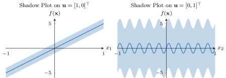
Most of the variation in this function is due to $x_{1}$, but there is a high frequency oscillation in $x_{2}$. As $f$ is additive in the two coordinates, we can identify a Lipschitz matrix ${\mathbf{L}}=\begin{bmatrix}5&0\\ 0&10\pi\end{bmatrix}$ by considering the largest derivative in each coordinate. Then applying Theorem 4.1, we would choose the active subspace $\operatorname{Span}\{{\mathbf{e}}_{2}\}$. However, as illustrated in Fig. 10, this yields much higher uncertainty than using $\operatorname{Span}\{{\mathbf{e}}_{1}\}$ because the oscillations in $x_{2}$ have less influence on the output than the linear term in $x_{1}$. We can remove the influence of these oscillations by using the $\epsilon$-Lipschitz matrix. Taking $\epsilon=2$, we can ignore the sine term and identify an $\epsilon$-Lipschitz matrix ${\mathbf{L}}_{2}=\begin{bmatrix}5&0\\ 0&0\end{bmatrix}$ With this choice, we choose the active subspace $\operatorname{Span}\{{\mathbf{e}}_{1}\}$. Although this has increased the uncertainty at each point, it yields better active subspace which reduces overall uncertainty.

Figure 10: Two shadow plots of the corrugated roof function Eq. 73. The solid line denotes the mean value, the shaded area denotes the area of possible oscillation.

8.3 Dimension Reduction

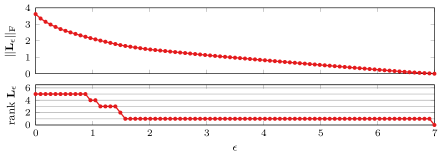
Just as we can use an $\epsilon$-Lipschitz matrix to remove undesirable oscillations, we can also use it for dimension reduction. If there is a subspace ${\mathcal{U}}$ on which a function varies by less than $\epsilon$, then there is an $\epsilon$-Lipschitz matrix that has a nullspace of $\dim({\mathcal{U}})$. We have no guarantee that by minimizing the Frobenius norm with the given function evaluations we will identify this low-rank $\epsilon$-Lipschitz matrix. However Figure 11 illustrates that we can sometimes find a low-rank matrix. In this example we note that by ignoring about $20\%$ of the variation, we can identify a rank-1 $\epsilon$-Lipschitz matrix.

Figure 11: With increasing $\epsilon$, we can identify low-rank $\epsilon$-Lipschitz matrices. This example shows the OTL Cirucit function where the $\epsilon$-Lipschitz matrix is estimated using 200 maximin samples chosen using an approximate Lipschitz matrix for this function.

References

- [1] M. S. Andersen, J. Dahl, and L. Vandenberghe, CVXOPT: A Python package for convex optimization, 2019, http://cvxopt.org.
- [2] C. B. Barber, D. P. Dobkin, and H. T. Huhdanpaa, The Quickhull algorithm for convex hulls, ACM T. Math. Software, 22 (1996), pp. 469–483, http://www.qhull.org.
- [3] E. N. Ben-Ari and D. M. Steinberg, Modeling data from computer experiments: An empirical comparison of kriging with MARS and projection pursuit regression, Qual Eng, 19 (2007), pp. 327–338, https://doi.org/10.1080/08982110701580930.
- [4] P. G. Constantine, Active Subspaces: Emerging Ideas for Dimension Reduction in Parameter Studies, SIAM, Philadelphia, 2015.
- [5] P. G. Constantine, A. Eftekhari, J. Hokanson, and R. A. Ward, A near-stationary subspace for ridge approximation, Comput. Methods Appl. Mech. Engrg., 326 (2017), pp. 402–421, https://doi.org/10.1016/j.cma.2017.07.038.
- [6] J. Cortés and F. Bullo, Coordination and geometric optimization via distributed dynamical systems, SIAM J. Control Optim., 44 (2005), pp. 1543–1574, https://doi.org/10.1137/S0363012903428652.
- [7] T. A. Davis and Y. Hu, The university of florida sparse matrix collection, ACM Trans. Math. Softw., 38 (2011), pp. 1–25, https://doi.org/10.1145/2049662.2049663.
- [8] D. L. Donoho, High-dimensional data analysis: The curses and blessings of dimensionality, in AMS Conference on Math Challenges of the 21st Century, 2000, http://citeseerx.ist.psu.edu/viewdoc/summary?doi=10.1.1.329.3392.
- [9] V. V. Fedorov, Theory of Optimal Experiments, Academic Press, New York, 1972.
- [10] A. I. J. Forrester, A. Sóbester, and A. J. Keane, Engineering Design via Surrogate Modelling: A Practical Guide, Wiley, 2008.
- [11] A. Glaws, P. G. Constantine, and R. D. Cook, Inverse regression for ridge recovery: a data-driven approach for parameter reduction in computer experiments, Statistics and Computing, 30 (2019), pp. 237–253, https://doi.org/10.1007/s11222-019-09876-y.
- [12] J. Golinski, Optimal synthesis problems solved by means of nonlinear programming and random methods, J. Mechanisms, (1970), pp. 287–309, https://doi.org/10.1016/0022-2569(70)90064-9.
- [13] W. V. Harper and S. K. Gupta, Sensitivity/uncertainty analysis of a borehole scenario comparing latin hypercube sampling and deterministic sensitivity approaches, tech. report, Battelle Memorial Institute, Oct. 1983.
- [14] J. M. Hokanson and P. G. Constantine, Data-driven polynomial ridge approximation using variable projection, SIAM J. Sci. Comput., 40 (2018), pp. A1566–A589, https://doi.org/10.1137/17M1117690.
- [15] A. Holiday, M. Kooshkbaghi, J. M. Bello-Rivas, C. William Gear, A. Zagaris, and I. G. Kevrekidis, Manifold learning for parameter reduction, Journal of Computational Physics, 392 (2019), pp. 419–431, https://doi.org/10.1016/j.jcp.2019.04.015.
- [16] R. A. Horn and C. R. Johnson, Matrix Analysis, Cambridge University Press, 2nd ed., 2013.
- [17] R. Kenett and S. Zacks, Modern Industrial Statistics: Design and Control of Quality and Reliability, Duxbury Press, Pacific Grove, CA, 1998.
- [18] R. B. Lehoucq, D. C. Sorensen, and C. Yang, ARPACK User’s Guide: Solution of Large-Scale Eigenvalue Problems with Implicitly Restarted Arnoldi Methods, SIAM, Philadelphia, 1998, https://doi.org/10.1137/1.9780898719628.
- [19] S. R. Lindemann and P. Cheng, Iteratively locating Voronoi vertices for dispersion estimation, in Proceedings of the 2005 IEEE International Conference on Robotics and Automation, Apr. 2005, pp. 3862–3867, https://doi.org/10.1109/ROBOT.2005.1570710.
- [20] J. J. Moré and S. M. Wild, Estimating computational noise, SIAM J. Sci. Comput., 33 (2011), pp. 1292–1314.
- [21] W. G. Müller, Coffee-house designs, in Optimum Design 2000, A. Atkinson, B. Bogacka, and A. Zhigljavsky, eds., Kluwer, Dordrecht, 2001, ch. 21, pp. 241–248.
- [22] M. R. Osborne and G. A. Watson, An algorithm for minimax approximation in the nonlinear case, Comput. J., 12 (1969), pp. 63–68, https://doi.org/10.1093/comjnl/12.1.63.
- [23] A. Pinkus, Ridge Functions, Cambridge University Press, 2015, https://doi.org/10.1017/CBO9781316408124.
- [24] L. Pronzato, Minimax and maximin space-filling designs: some properties and methods for construction, J. Soc. Fr. Stat., 158 (2017), pp. 7–36, http://journal-sfds.fr/article/view/601.
- [25] C. E. Rasmussen and C. K. I. Williams, Gaussian Processes for Machine Learning, MIT Press, 2006.
- [26] J. C. Regier and P. B. Stark, Mini-minimax uncertainty quantification for emulators, SIAM/ASA J. Uncert. Quant., 3 (2015), pp. 686–708, https://doi.org/10.1137/130917909.
- [27] A. Saltelli, M. Ratto, T. Andres, F. Campolongo, J. Cariboni, D. Gatelli, M. Saisana, and S. Tarantola, Global Sensitivity Analysis: The Primer, John Wiley & Sons, New York, 2008.
- [28] T. J. Santer, B. J. Williams, and W. I. Notz, The Design and Analysis of Computer Experiments, Springer, 2003.
- [29] I. Sobol’, S. Tarantola, D. Gatelli, S. Kucherenko, and W. Mauntz, Estimating the approximation error when fixing unessential factors in global sensitivity analysis, Reliability Engineering & System Safety, 92 (2007), pp. 957–960, https://doi.org/10.1016/j.ress.2006.07.001.
- [30] E. Stinstra, D. den Hertog, P. Stehouwer, and A. Vestjens, Constrained maximin designs for computer experiments, Technometrics, 45 (2003), pp. 340–346, https://doi.org/10.1198/004017003000000168.
- [31] A. G. Sukharev, Minimax models in the theory of numerical methods, Springer Science+Business Media, 1992.
- [32] S. Surjanovic and D. Bingham, Virtual library of simulation experiments: Test functions and datasets, 2013, http://www.sfu.ca/~ssurjano.
- [33] A. Suzuki and Z. Drezner, The -center location problem in an area, Locat. Sci., 4 (1996), pp. 69–82, https://doi.org/10.1016/S0966-8349(96)00012-5.
- [34] J. F. Traub and A. G. Werschulz, Complexity and Information, Cambridge University Press, Cambridge, 1998.
- [35] J. F. Traub, H. Woźniakowski, and G. W. Wasilkowski, Information-Based Complexity, Academic Press, 1988.
- [36] Y. Wu, Lecture notes for ECE598YW: Information-theoretic methods for high-dimensional statistics, http://www.stat.yale.edu/~yw562/teaching/it-stats.pdf.