A modified version of the IEEE 3-area RTS ’96 Test Case for time series analysis

Abstract

This report describes a modified version of the IEEE 3-area RTS ’96 Test Case for time series analysis. This test case was originally developed to investigate the impact of the introduction of losses in the market clearing, thus the main application of this system is DC Optimal Power Flow (OPF) studies. A fourth area is included in the system. In each snapshot, wind power production and load consumption are modified. This allows for different import-export situations among zones, varying the prices in each zone. Moreover, several High-Voltage Direct-Current (HVDC) lines are included in the system.

I Introduction

In the last decades, over 25,000 km of High-Voltage Direct-Current (HVDC) lines have been gradually integrated to the existing pan-European HVAC system. Thanks to their properties, HVDC lines facilitate the transfer of bulk power over long distances, allow the connection of asynchronous areas, represent a cost-effective solution for long-distance submarine cables and provide a useful tool for power systems stability. HVAC-HVDC interaction will be a key feature in the coming years, both for system operation and system reliability.

In this regard, there are few test systems which include meshed HVDC links. This report presents a modified version of the IEEE RTS ’96 Test System [1], with the inclusion of several HVDC interconnectors. The intention is to develop a test system with universal characteristics, to be used as a reference for testing the impact of different evaluation techniques on diverse applications and technologies. This test system was used for the first time in [2], for analyzing the impact of the introduction of HVDC losses in the market clearing algorithm of zonal pricing markets.

The test case is modified as follows:

• A fourth area is included.

• Three new VSC-based HVDC links are included to connect Area 1 to the other areas.

• Different wind farms are added in each area; different wind profiles are considered.

• All the loads are considered elastic; three different load profiles are considered.

• To create high and low price areas, generator costs and load utilities in the four areas are multiplied by scaling factors.

• To create price differences over the year, load consumption and wind generation vary in each snapshot.

II System Topology

This test case is intended to represent a power system where zonal pricing is applied. For this reason, the system is a multi-area power system developed by merging four different areas, each of which is the IEEE RTS 24-bus Test System shown in Figure 1. The whole system is represented in Figure 2. The four areas are interconnected by the following new interconnectors:

• 400 kV VSC-HVDC line connecting bus # 106 and bus # 203;

• 250 kV VSC-HVDC line connecting bus # 123 and bus # 323;

• 350 kV VSC-HVDC line connecting bus # 121 and bus # 422;

• 230 kV AC line connecting bus # 222 and bus # 317;

• 138 kV AC line connecting bus # 307 and bus # 403;

• 230 kV AC line connecting bus # 313 and bus # 415;

• 230 kV AC line connecting bus # 323 and bus # 417;

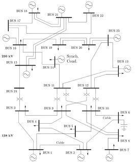
Figure 1: IEEE RTS 24-bus Test System.

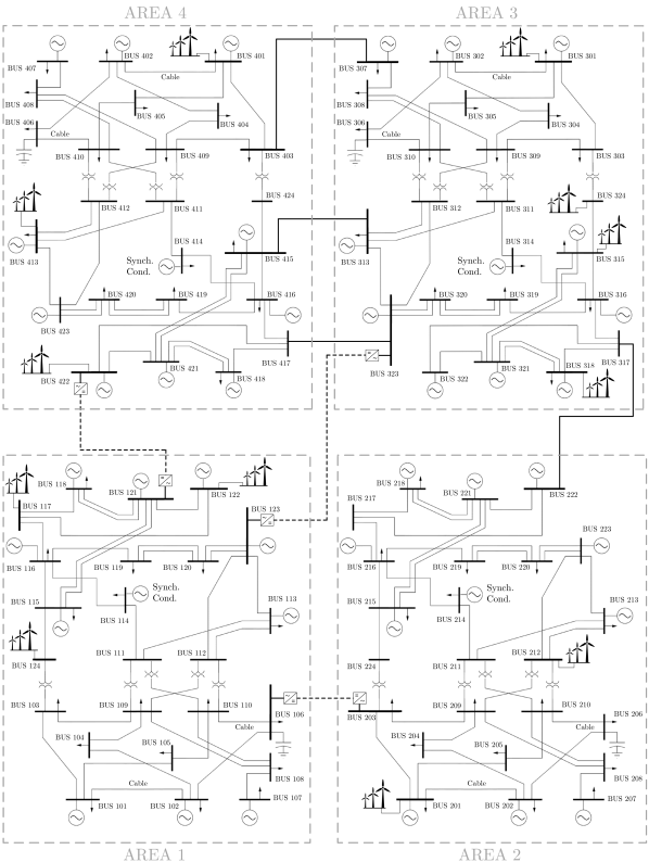
Figure 2: 4-area 96-bus system.

III Bus Data

The bus data is obtained from the IEEE RTS ’96 Test Stystem [1]. The four areas are labeled with numbers raging from 1 to 4. The buses in each area are numbered with a preassigned numbering system (e.g., in Area 1, the 24 buses are labeled with number raging from 101 to 124, in Area 2 from 201 to 224, and so on). The slack bus is Bus # 113 in Area 1. The bus data for Area 1 and 2 is listed in Table I. Area 3 and 4 are equal to Area 2. The bus types are the following:

• 1 - load bus;

• 2 - generator bus;

• 3 - slack bus.

TABLE I: bus data (area 1 and 2)

AREA	BUS	BUS			Base	V	V
#	#	TYPE	GL	BL	kV	max	min
1	101	2	0	0	138	1.05	0.95
1	102	2	0	0	138	1.05	0.95
1	103	1	0	0	138	1.05	0.95
1	104	1	0	0	138	1.05	0.95
1	105	1	0	0	138	1.05	0.95
1	106	1	0	100	138	1.05	0.95
1	107	2	0	0	138	1.05	0.95
1	108	1	0	0	138	1.05	0.95
1	109	1	0	0	138	1.05	0.95
1	110	1	0	0	138	1.05	0.95
1	111	1	0	0	230	1.05	0.95
1	112	1	0	0	230	1.05	0.95
1	113	3	0	0	230	1.05	0.95
1	114	2	0	0	230	1.05	0.95
1	115	2	0	0	230	1.05	0.95
1	116	2	0	0	230	1.05	0.95
1	117	1	0	0	230	1.05	0.95
1	118	2	0	0	230	1.05	0.95
1	119	1	0	0	230	1.05	0.95
1	120	1	0	0	230	1.05	0.95
1	121	2	0	0	230	1.05	0.95
1	122	2	0	0	230	1.05	0.95
1	123	2	0	0	230	1.05	0.95
1	124	1	0	0	230	1.05	0.95
2	201	2	0	0	138	1.05	0.95
2	202	2	0	0	138	1.05	0.95
2	203	1	0	0	138	1.05	0.95
2	204	1	0	0	138	1.05	0.95
2	205	1	0	0	138	1.05	0.95
2	206	1	0	100	138	1.05	0.95
2	207	2	0	0	138	1.05	0.95
2	208	1	0	0	138	1.05	0.95
2	209	1	0	0	138	1.05	0.95
2	210	1	0	0	138	1.05	0.95
2	211	1	0	0	230	1.05	0.95
2	212	1	0	0	230	1.05	0.95
2	213	2	0	0	230	1.05	0.95
2	214	2	0	0	230	1.05	0.95
2	215	2	0	0	230	1.05	0.95
2	216	2	0	0	230	1.05	0.95
2	217	1	0	0	230	1.05	0.95
2	218	2	0	0	230	1.05	0.95
2	219	1	0	0	230	1.05	0.95
2	220	1	0	0	230	1.05	0.95
2	221	2	0	0	230	1.05	0.95
2	222	2	0	0	230	1.05	0.95
2	223	2	0	0	230	1.05	0.95
2	224	1	0	0	230	1.05	0.95

GL and BL refer to the real and imaginary components of the shunt admittance to ground, Base kV to the voltage level, Vmax and Vmin to the maximum allowed voltage deviation.

IV Elastic loads

In each area, 17 elastic load are included. Their location and their peak values are taken from the IEEE RTS ’96 Test System [1] (peak values increased by 10%), their utilities are linear and derived from [3]. The load data is listed in Table II. To create high and low price areas, load utilities in the four areas are multiplied by a scaling factor, respectively 1.8, 0.95, 1 and 1.1.

In order to create price differences over the year, the maximum consumption of loads varies according to their yearly and daily profiles (see Figure 3). Three different types of load are considered: residential, industrial and commercial. The profiles are assigned to the loads using the coefficients $i_{1}$ and $i_{2}$, as shown in Table II. The maximum consumption is modified as follows:

$$\begin{split}&D^{max}=0.65\cdot\textsc{res}_{y}\textsc{res}_{d}\,r\,i_{1}\overline{D}^{max}\,\,+\\ &\qquad\qquad 0.35\cdot\textsc{com}_{y}\textsc{com}_{d}\,r\,i_{1}\overline{D}^{max}\,\,+\\ &\qquad\qquad\textsc{ind}_{y}\textsc{ind}_{d}\,r\,i_{2}\overline{D}^{max},\end{split}$$ (1)

where $r$ is a random numbers between 0.95 and 1.05, $i_{1}$ and $i_{2}$ are either 0 or 1 according to the load profile, $\textsc{res}_{y}$, $\textsc{res}_{d}$, $\textsc{com}_{y}$, $\textsc{com}_{d}$, $\textsc{ind}_{y}$ and $\textsc{ind}_{d}$ are the different yearly and daily coefficients, listed in Table III and IV, and $\overline{D}^{max}$ is the peak load, shown in Table II.

TABLE II: load data

LOAD	BUS	Peak Load	Utility
ID	#	(MW)	($/MWh)	$i_{1}$	$i_{2}$
D01	1	118.8	39.21	0	1
D02	2	106.7	35.21	1	$0$
D03	3	198	65.35	1	$0$
D04	4	81.4	26.89	0	$1$
D05	5	78.1	25.79	1	$0$
D06	6	149.6	49.42	1	$0$
D07	7	137.5	45.42	0	$1$
D08	8	188.1	62.11	1	$0$
D09	9	192.5	63.56	0	$1$
D10	10	214.5	80.82	1	$0$
D11	13	291.5	96.97	0	$1$
D12	14	213.4	70.45	1	$0$
D13	15	348.7	112.07	0	$1$
D14	16	110	36.34	1	$0$
D15	18	366.3	135.88	0	$1$
D16	19	199.1	65.71	1	$0$
D17	20	140.8	46.49	1	0

Figure 3: Load profiles.

TABLE III: yearly load profiles

Period	$RES_{y}$	$IND_{y}$	$COM_{y}$
Jan 1 - Jan 15	0.620	0.731	0.683
Jan 16 - Jan 31	0.560	0.700	0.620
Feb 1 - Feb 14	0.524	0.692	0.601
Feb 15 - Feb 28	0.490	0.710	0.630
Mar 1 - Mar 15	0.476	0.769	0.654
Mar 16 - Mar 31	0.500	0.787	0.730
Apr 1 - Apr 15	0.571	0.792	0.774
Apr 16 - Apr 30	0.620	0.820	0.790
May 1 - May 15	0.643	0.862	0.824
May 16 - May 31	0.720	0.890	0.860
Jun 1 - Jun 15	0.857	0.940	0.940
Jun 16 - Jun 30	0.910	0.960	0.950
Jul 1 - Jul 15	0.952	0.962	0.940
Jul 16 - Jul 31	0.955	0.975	0.947
Aug 1 - Aug 15	0.976	0.977	0.955
Aug 16 - Aug 31	0.999	0.992	0.980
Sep 1 - Sep 15	1.000	1.000	1.000
Sep 16 - Sep 30	0.940	0.930	0.900
Oct 1 - Oct 15	0.730	0.820	0.780
Oct 16 - Oct 31	0.580	0.810	0.753
Nov 1 - Nov 15	0.550	0.846	0.740
Nov 16 - Nov 30	0.570	0.820	0.680
Dec 1 - Dec 15	0.610	0.754	0.660
Dec 16 - Dec 31	0.615	0.740	0.670

TABLE IV: daily load profiles

Hour	$RES_{d}$	$IND_{d}$	$COM_{d}$
00-01	0.600	0.150	0.040
01-02	0.480	0.140	0.050
02-03	0.420	0.110	0.060
03-04	0.380	0.090	0.070
04-05	0.350	0.100	0.080
05-06	0.360	0.115	0.090
06-07	0.400	0.220	0.110
07-08	0.460	0.350	0.140
08-09	0.510	0.620	0.170
09-10	0.530	0.850	0.200
10-11	0.530	0.900	0.280
11-12	0.540	0.880	0.380
12-13	0.580	0.870	0.500
13-14	0.560	0.910	0.560
14-15	0.540	0.950	0.670
15-16	0.550	0.960	0.850
16-17	0.610	0.820	0.870
17-18	0.830	0.600	0.870
18-19	0.960	0.420	0.890
19-20	1.000	0.370	0.850
20-21	0.950	0.380	0.700
21-22	0.900	0.310	0.600
22-23	0.790	0.190	0.450
23-24	0.810	0.160	0.220

V Generating units

In each area, 33 generating units are included. Their data is taken from the IEEE RTS ’96 Test System [1] and listed in Table V. The minimum output level of all generating units has been set to zero. The cost of production of each unit is assumed to be a linear function of their output level. As for loads, these costs are multiplied by different scaling factors, respectively 0.97, 1.03, 1 and 0.99, according to the area where generators are located in. Start-up and shut-down costs, unit cylce restrictions, ramping rates and emissions have not been considered. Unit G15 is a synchronous condenser.

TABLE V: generator data

UNIT	BUS	P max	Q min	Q max	Cost
ID	#	(MW)	(MVAR)	(MVAR)	($/MWh)
G01	1	20	0	10	130
G02	1	20	0	10	130.00
G03	1	76	-25	30	16.08
G04	1	76	-25	30	16.08
G05	2	20	0	10	130.00
G06	2	20	0	10	130.00
G07	2	76	-25	30	16.08
G08	2	76	-25	30	16.08
G09	7	100	0	60	43.66
G10	7	100	0	60	43.66
G11	7	100	0	60	43.66
G12	13	197	0	80	48.58
G13	13	197	0	80	48.58
G14	13	197	0	80	48.58
G15	14	0	-50	200	0.00
G16	15	12	0	6	56.56
G17	15	12	0	6	56.56
G18	15	12	0	6	56.56
G19	15	12	0	6	56.56
G20	15	12	0	6	56.56
G21	15	155	-50	80	12.39
G22	16	155	-50	80	12.39
G23	18	400	-50	200	4.42
G24	21	400	-50	200	4.42
G25	22	50	-10	16	1E-04
G26	22	50	-10	16	1E-04
G27	22	50	-10	16	1E-04
G28	22	50	-10	16	1E-04
G29	22	50	-10	16	1E-04
G30	22	50	-10	16	1E-04
G31	23	155	-50	80	12.39
G32	23	155	-50	80	12.39
G33	23	350	-25	150	11.85

TABLE VI: wind farm data

AREA	BUS	P max	Wind
#	#	(MW)	coefficient
1	117	113.5	DK1
1	122	56.75	DK1
1	122	56.75	DK1
1	124	113.5	DK1
2	201	17.03	DK2
2	212	8.51	DK2
2	212	8.52	DK2
3	301	34.05	SE1
3	301	34.05	SE1
3	315	68.1	SE1
3	317	68.1	SE1
3	324	68.1	SE1
4	401	17.25	SE4
4	401	17.25	SE4
4	413	34.05	SE4
4	422	34.05	SE4

VI Wind farms

In each area, several wind farms are included. Their data is listed in Table VI. No uncertainty is considered: the output of the wind farm is known, and it varies according to the wind profile of each area. In order to have reasonable wind profiles, they are based on the wind power production of DK1, DK2 [4], SE1 and SE4 [5] in 2016. The four wind profiles are depicted in Figure 4.

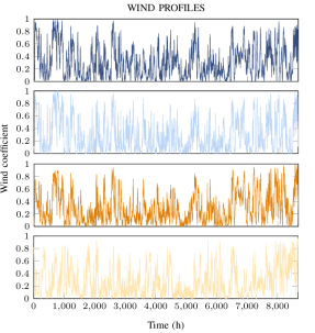
Figure 4: Wind profiles. From the top: Area 1 (DK1), Area 2 (DK2), Area 3 (SE1) and Area 4 (SE4) [4, 5].

VII Transmission system

The internal network of each area is a meshed AC grid with 31 overhead lines, 2 cables and 5 transformers (see Figure 1). Transmission network data is obtained from the IEEE RTS ’96 Test System [1] and listed in Table VII. Only continuous line ratings are considered.

The four area are interconnected by the following AC and HVDC tie-lines:

• 400 kV VSC-HVDC line connecting bus # 106 and bus # 203;

• 250 kV VSC-HVDC line connecting bus # 123 and bus # 323;

• 350 kV VSC-HVDC line connecting bus # 121 and bus # 422;

• 230 kV AC line connecting bus # 222 and bus # 317;

• 138 kV AC line connecting bus # 307 and bus # 403;

• 230 kV AC line connecting bus # 313 and bus # 415;

• 230 kV AC line connecting bus # 323 and bus # 417;

The four AC interconnectors are adopted from [1], their data is listed in Table VIII. The base power is $100\text{\,}\mathrm{M}\mathrm{W}$ and the base voltage $230\text{\,}\mathrm{kV}$ (except for line 307-403, for which the base voltage is $138\text{\,}\mathrm{kV}$).

Three HVDC interconnectors are connecting Area 1 to the other areas. The base power is $100\text{\,}\mathrm{M}\mathrm{W}$ and the base voltages (DC side) respectively $400\text{\,}\mathrm{kV}$, $250\text{\,}\mathrm{kV}$ and $350\text{\,}\mathrm{kV}$. The converter station losses are represented with the generalized loss model [6, 7]:

$$p^{loss}_{conv}=a\,\left|I_{conv}\right|^{2}+b\,\left|I_{conv}\right|+c,$$ (2)

where $a$, $b$ and $c$ are numerical parameters reflecting the quadratic, linear and constant dependence of the losses on the line current and $\left|I^{conv}\right|$ is the magnitude of the current flowing through the converter. The data of HVDC interconnectors is derived from [7] and listed in Table IX.

It is worth mentioning that, since Area 1 is connected to the other areas only through HVDC lines, the whole system can represent two asynchronous areas (Area 1 and Area 2-4).

TABLE VII: line data

	FROM	TO	R	X	B	Rating	Transf
ID	BUS	BUS	(pu)	(pu)	(pu)	(MVA)	ratio
C01	1	2	0.003	0.014	0.461	175	0
L01	1	3	0.055	0.211	0.057	175	0
L02	1	5	0.022	0.085	0.023	175	0
L03	2	4	0.033	0.127	0.034	175	0
L04	2	6	0.050	0.192	0.052	175	0
L05	3	9	0.031	0.119	0.032	175	0
T01	3	24	0.002	0.084	0.000	400	1.03
L06	4	9	0.027	0.104	0.028	175	0
L07	5	10	0.023	0.088	0.024	175	0
C02	6	10	0.014	0.061	2.459	175	0
L08	7	8	0.016	0.061	0.017	175	0
L09	8	9	0.043	0.165	0.045	175	0
L10	8	10	0.043	0.165	0.045	175	0
T02	9	11	0.002	0.084	0.000	400	1.03
T03	9	12	0.002	0.084	0.000	400	1.03
T04	10	11	0.002	0.084	0.000	400	1.02
T05	10	12	0.002	0.084	0.000	400	1.02
L11	11	13	0.006	0.048	0.100	500	0
L12	11	14	0.005	0.042	0.088	500	0
L13	12	13	0.006	0.048	0.100	500	0
L14	12	23	0.012	0.097	0.203	500	0
L15	13	23	0.011	0.087	0.182	500	0
L16	14	16	0.005	0.039	0.082	500	0
L17	15	16	0.002	0.017	0.036	500	0
L18	15	21	0.006	0.049	0.103	500	0
L19	15	21	0.006	0.049	0.103	500	0
L20	15	24	0.007	0.052	0.109	500	0
L21	16	17	0.003	0.026	0.055	500	0
L22	16	19	0.003	0.023	0.049	500	0
L23	17	18	0.002	0.014	0.030	500	0
L24	17	22	0.014	0.105	0.221	500	0
L25	18	21	0.003	0.026	0.055	500	0
L26	18	21	0.003	0.026	0.055	500	0
L27	19	20	0.005	0.040	0.083	500	0
L28	19	20	0.005	0.040	0.083	500	0
L29	20	23	0.003	0.022	0.046	500	0
L30	20	23	0.003	0.022	0.046	500	0
L31	21	22	0.009	0.068	0.142	500	0

TABLE VIII: AC interconnector data

LINE	FROM	TO	R	X	B	Rating
ID	BUS	BUS	(pu)	(pu)	(pu)	(MVA)
AC01	222	317	0.013	0.104	0.218	500
AC02-1	307	403	0.042	0.161	0.044	175
AC02-2	313	415	0.010	0.075	0.158	500
AC02-3	323	417	0.010	0.074	0.155	500

TABLE IX: HVDC interconnector data

LINE	FROM	TO	R	$a_{inv}$	$a_{rec}$	$b$	$c$	Rating
ID	BUS	BUS	(pu)	(pu)	(pu)	(pu)	(pu)	(MW)
DC01	106	203	.0080	.0005	.0003	.0007	.0074	80
DC02	123	323	.0036	.0056	.0019	.0013	.0015	400
DC03	121	422	.0037	.0049	.0019	.0012	.0015	600

VIII Flow-based Market Coupling

Figure 5: Equivalent representation of the system under the assumption of FBMC.

In a zonal pricing system, the network is split into price-zones in case of congestion on certain flowgates. The intra-zonal network is not included in the model, and a single price per zone is defined. The main difference between nodal and zonal pricing is that, in case of congestion, in a nodal pricing market all the nodes are subjected to different prices, while in a zonal pricing market price differences arise only among zones, with all generators and loads subjected to their zonal price [3]. An evolution of zonal pricing is the Flow-Based Market Coupling (FBMC), which aims at coupling different independent markets. FBMC includes two clearing processes: first the energy market clearing, where a clearing price per zone is determined according to the internal power exchanges, and second, the import and export trades via the interconnections [3]. As for zonal pricing, the intra-zonal flows are not represented in the model; in addition, cross-border lines to another zone are aggregated into a single equivalent interconnector.

Under the assumption of FBMC, all the intra-zonal nodes are aggregated into a single equivalent node. As a consequence, the 96-bus system is reduced to a 4-area system, as shown in Figure 5. Also, all the AC tie-lines connecting Area 3 to Area 4 are substituted by a single equivalent interconnector.

IX Conclusion

This report presents a modified version of the IEEE RTS ’96 Test System [1], with the inclusion of several HVDC interconnectors, for time series analyses. The test case is modified introducing a fourth area, three new VSC-based HVDC links, different wind farms and elastic loads. The intent is to develop a test system with universal characteristics, to be used as a reference for testing the impact of different evaluation techniques on diverse applications and technologies. The test case is designed for DC Optimal Power Flow (OPF) studies and used for the first time in [2].

References

- [1] C. Grigg, P. Wong et al., “The IEEE Reliability Test System-1996. A report prepared by the Reliability Test System Task Force of the Application of Probability Methods Subcommittee,” IEEE Transactions on Power Systems, vol. 14, no. 3, pp. 1010–1020, Aug 1999.
- [2] A. Tosatto, T. Weckesser, and S. Chatzivasileiadis, “Market Integration of HVDC Lines,” arXiv.org, December 2018. Available: https://arxiv.org/pdf/1812.00734v1.pdf.
- [3] T. Krause, Evaluating Congestion Management Schemes in Liberalized Electricity Markets Applying Agent-based Computational Economics. Doctoral thesis, Swiss Federal Institute of Technology, Zürich, Switzerland, 2006.
- [4] Nord Pool Group. Historical Market Data - Wind Power Production DK 2016. [Online]. Available: https://www.nordpoolgroup.com/globalassets/marketdata-excel-files/wind-power-dk_2016_hourly.xls [Accessed: 2018-09-28]
- [5] Nord Pool Group. Historical Market Data - Wind Power Production SE 2016. [Online]. Available: https://www.nordpoolgroup.com/globalassets/marketdata-excel-files/wind-power-se_2016_hourly.xls [Accessed: 2018-09-28]
- [6] G. Daelemans, VSC HVDC in meshed networks. Master’s thesis, Katholieke Universiteit Leuven, Leuven, Belgium, 2008.
- [7] J. Beerten, S. Cole, and R. Belmans, “Generalized Steady-State VSC MTDC Model for Sequential AC/DC Power Flow Algorithms,” IEEE Transactions on Power Systems, vol. 27, no. 2, pp. 821–829, May 2012.