The Grism Lens-Amplified Survey from Space (GLASS). XIII. G800L optical spectra from the parallel fields

Abstract

We present a catalogue of 22755 objects with slitless, optical, Hubble Space Telescope (HST) spectroscopy from the Grism Lens-Amplified Survey from Space (GLASS). The data cover $\sim$220 sq. arcmin to 7-orbit ($\sim$10 ks) depth in 20 parallel pointings of the Advanced Camera for Survey’s G800L grism. The fields are located 6^′ away from 10 massive galaxy clusters in the HFF and CLASH footprints. Thirteen of the fields have ancillary HST imaging from these or other programs to facilitate a large number of applications, from studying metal distributions at $z\sim 0.5$, to quasars at $z\sim 4$, to the star formation histories of hundreds of galaxies in between. The spectroscopic catalogue has a median redshift of $\langle z\rangle=0.60$ with a median uncertainty of $\Delta z/(1+z)\lesssim 2\%$ at $\rm F814W\lesssim 23$ AB. Robust continuum detections reach a magnitude fainter. The 5 $\sigma$ limiting line flux is $f_{\rm lim}\approx 5\times 10^{-17}\rm~{}erg~{}s^{-1}~{}cm^{-2}$ and half of all sources have 50% of pixels contaminated at $\lesssim$1%. All sources have 1- and 2-D spectra, line fluxes/uncertainties and identifications, redshift probability distributions, spectral models, and derived narrow-band emission line maps from the Grism Redshift and Line Analysis tool (GRIZLI). We provide other basic sample characterisations, show data examples, and describe sources and potential investigations of interest. All data and products will be available online along with software to facilitate their use.

1 Introduction

The Hubble Space Telescope (HST) provides some of the best ultraviolet (UV) to near-infrared (NIR) imaging available. These data underpin most of our knowledge of the distant universe. Ground-based spectra—from, e.g., MOSDEF (Kriek et al., 2015) and LEGA-C (van der Wel et al., 2016)—are critical, but the atmosphere limits continuum measurements to the most massive galaxies and blurs all spatial information. Using space-based data reduces these restrictions and yields a clearer picture of galaxy evolution.

HST’s slitless grisms have played key roles here. They produce maps of every source at every wavelength at spatial scales inaccessible from Earth without adaptive optics. The two NIR grisms—G102 and G141 on WFC3—have proven especially effective, with, e.g., the 3D-HST survey (Momcheva et al., 2016) and our own Grism Lens-Amplified Survey from Space (GLASS; Schmidt et al., 2014; Treu et al., 2015) providing rest-optical $z>1$ spectroscopy over scores to hundreds of sq. arcmin without the need for potentially biasing photometric preselection or slit masks. Paired with HST imaging, these data have extended our knowledge of the ages and star formation histories of galaxies at early cosmic times in ways comparable to ground based results at $z\lesssim 1$ (e.g., Whitaker et al., 2012; Newman et al., 2014; Nelson et al., 2016; Wang et al., 2017, 2018; Abramson et al., 2018; Morishita et al., 2018a, b).

Table 1: Basic survey information for the 20 GLASS ACS parallels. Field names reflect GLASS central pointing/IR grism (cluster) IDs and ROOT is the corresponding catalog keyword (Appendix A.2). PAs are “PA_V3.”
^a All objects with ${\rm c}|z-z_{\rm cl}|(1+z_{\rm cl})^{-1}<2000~{}\rm km\,s^{-1}$ irrespective of $z_{Q}$ where $z_{\rm cl}$ is the GLASS cluster redshift from Table 1 of Treu et al. (2015).
^b Covering band(s) other than F814W to support SED fitting.
^c CLASH – Postman et al. (2012); http://archive.stsci.edu/proposal_search.php?mission=hst&id=12067; HFF – Lotz et al. (2017); http://archive.stsci.edu/proposal_search.php?mission=hst&id=13498; Ebeling – GO10420; http://archive.stsci.edu/proposal_search.php?mission=hst&id=10420; Riess – GO13063; http://archive.stsci.edu/proposal_search.php?mission=hst&id=13063; Rodney – GO13386; http://archive.stsci.edu/proposal_search.php?mission=hst&id=13386; Siana – GO13389; http://archive.stsci.edu/proposal_search.php?mission=hst&id=13389.
^d One band.
^e Grism data incorporated from GO12099 (PI Riess).

Field	ROOT	RA [J2000]	DEC [J2000]	PA [deg]	$N_{\rm srcs}$	$N_{\rm infall}$a	G800L Exptime [s]	HST Imaging [program or PI]b,c
Abell 2744	j0014m3023	0:13:53.9	-30:22:51	323	976	26	10076	HFF, Siana, Rodney
Abell 2744	j0014m3030	0:14:20.9	-30:29:46	225	1066	16	10076	HFFd, Rodneyd
Abell 370	j0240m0132	2:39:31.6	-1:31:42	343	1028	31	10076	$\cdots$
Abell 370	j0240m0140	2:39:44.6	-1:40:08	245	965	32	10344	$\cdots$
MACS0416	j0416m2402	4:15:44.7	-24:02:04	337	808	15	10076	CLASH, Rodney
MACS0416	j0416m2410	4:15:56.0	-24:09:42	254	887	24	10186	$\cdots$
MACS0717	j0717p3750	7:17:16.3	37:49:53	10	1123	46	9927	HFF, CLASH, Siana, Ebeling
MACS0717	j0718p3747	7:18:01.6	37:47:26	110	1186	37	10061	$\cdots$
MACS0744	j0745p3922	7:45:08.6	39:22:16	194	853	37	9562	CLASH
MACS0744	j0745p3930	7:45:20.6	39:30:10	109	934	35	10061	$\cdots$
MACS1149	j1150p2218	11:49:40.3	22:18:02	215	1117	37	10084	HFF, CLASHd, Siana
MACS1149	j1150p2225	11:50:00.9	22:25:25	122	1090	47	9854	CLASH
RXJ1347	j1347m1140	13:47:19.7	-11:40:11	13	1049	31	10076	CLASH
RXJ1347	j1347m1147	13:47:09.4	-11:47:36	293	954	20	10344	$\cdots$
MACS1423	j1424p2401	14:24:06.8	24:00:38	178	813	40	10076	CLASH
MACS1423	j1424p2408	14:24:09.4	24:08:19	98	939	33	10344	$\cdots$
MACS2129	j2130m0736	21:29:31.5	-7:35:40	58	1131	39	10061	Rodney
MACS2129e	j2130m0742	21:29:54.4	-7:41:45	136	3910	127	18789	CLASH, Riess
RXJ2248	j2249m4433	22:49:18.0	-44:32:37	143	906	16	9372	HFF, CLASH, Riess
RXJ2248	j2249m4438	22:48:46.0	-44:37:39	223	1020	27	10344	CLASHd

Beyond their scientific utility, HST’s grisms play a pathfinding role: the astronomical community has decided that space-based, wide-field, slitless spectroscopy will be an increasingly large part of its portfolio with the forthcoming operation of JWST, Euclid, and WFIRST. Hence, building intuition, applications, and tools to handle these data is prudent.

HST’s less widely used optical disperser—the ACS G800L grism—is powerful in this context. Covering $\lambda=0.5$–1.0 µm with $\sim$2.5$\times$ WFC3’s footprint, G800L extends space-based grism surveys to lower redshifts and more than doubles their area. The instrument’s capability has been exploited by the GRAPES (GO9793, PI Malhotra; Pirzkal et al., 2004) and PEARS (GO10530, PI Malhotra; Straughn et al., 2008, 2009) surveys, and 3D-HST, with all results obtained prior to 3D-HST compiled by Kümmel et al. (2011).

Here, we describe GLASS’ use of the G800L grism in parallel observing mode and present a source catalogue covering the 20 fields this survey comprises to 7-orbit depth (cf. 2 orbits for 3D-HST). These data may be useful to anyone interested in a range of scientific questions—from infalling cluster galaxies to $z\gtrsim 4$ Lyman-$\alpha$ emitters—and illustrate what could be done with higher signal-to-noise ratio ($S/N$) or spectral resolution data from future facilities.

Below, Section 2 describes data acquisition, field locations, reduction procedures, and output products. Section 3 describes the catalogue’s redshift, magnitude, and contamination distributions, and highlights some notable sources for further study. Section 4 proposes some uses of the data. Section 5 summarises. We provide file descriptions and some useful pieces of code in the Appendix. Throughout, we take $(H_{0}~{}\mathrm{km^{-1}~{}s}~{}{\rm Mpc},\Omega_{m},\Omega_{\Lambda})=(70,0.3,0.7)$ and quote AB magnitudes (Oke, 1974). All data/products are available upon request and will be made public.

2 Data

2.1 Acquisition

GLASS covers ten $z\sim 0.4$–0.6 cluster sightlines: six from HFF (Lotz et al., 2017) and four more from CLASH (Postman et al., 2012). WFC3 was placed on the cluster centre at each sightline where gravitational lensing maximises the chances of detecting high-redshift Lyman-$\alpha$ emitters. G102 and G141 were exposed there in series for 5 + 2 orbits, respectively. This process was repeated in two visits at two roughly orthogonal position angles (PAs) to facilitate source deblending. A $2\times$2 dither pattern with sub-pixel offsets was used to support image interlacing (Brammer et al., 2012), the format of the GLASS IR coadds.

In parallel with the NIR grism observations, G800L was exposed to a region $\sim$6^′ ($\sim$2 Mpc) away from the cluster centres. Given HST’s rotation between visits, this strategy yielded 20, non-overlapping G800L survey fields; i.e., a spectroscopic database covering $\sim$220 sq. arcmin to 7-orbit ($\sim$10 ks) depth. Data were acquired between 24 December 2013 and 18 January 2015. Table 1 provides basic information.

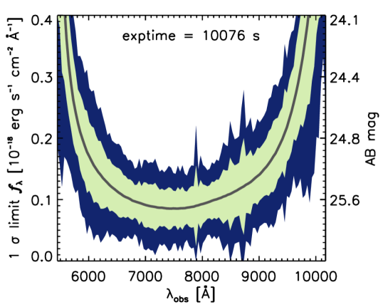
Figure 1: GLASS G800L sensitivity based on a $1^{\prime\prime}$ spatial extraction aperture. This plot describes Abell 2744 (at PA 323) but is typical of all pointings. Thresholds are the median 1 $\sigma$ $f_{\lambda}$ limit (grey) and that value’s 1 $\sigma$ and 2 $\sigma$ scatter (shaded). The median 5 $\sigma$ limiting line flux is $f_{\rm lim}\approx 5\times 10^{-17}\,{\rm erg~{}s^{-1}~{}cm^{-2}}$ ($\log f_{\rm lim}=-16.29\pm 0.36$).

A F814W pre-image was taken with each grism exposure (2 per orbit per PA). These data are necessary for source detection, spectral ID assignment, and wavelength calibration. Where possible, one PA was aligned with planned or actual ancillary imaging. This was achieved in 13 fields, where GLASS’ F814W pre-images complement or supplement other HST photometry (Table 1). GLASS pre-images are the only HST images in the remainder (e.g., MACS0717 j0718p3747). We provide example spectrophotometry in Section 4.2 and catalogue matching instructions in Appendix B, but all analyses here including redshift estimation use no additional photometry unless stated.

2.2 Reduction

Whereas the GLASS NIR data (Schmidt et al., 2014; Treu et al., 2015) were reduced using a modified version of the 3D-HST pipeline (Brammer et al., 2012; Momcheva et al., 2016), the ACS parallel data were extracted using a python package with improved capabilities: GRIZLI—the Grism Redshift and Line Analysis tool (see Wang et al., 2017, 2018, Brammer et al. in preparation). As with the original pipeline, the basic ingredients are two full-field ACS frames: one direct image, and one containing the dispersed 2D spectra of all sources therein. The former serves as the reference frame to which the latter is anchored.

GRIZLI first identifies cosmic rays in the F814W and G800L exposures using standard settings with the AstroDrizzle software (Gonzaga & et al., 2012), and fits and removes a two dimensional master sky image from the grism exposures. We refine the astrometric alignment including both a fine relative alignment between exposures and a global alignment to an absolute reference frame, here defined by the GAIA DR2 catalogue (Gaia Collaboration et al., 2018). As there are no telescope offsets between the paired F814W direct and G800L grism exposures, the alignment of the former is applied directly to the latter. Finally, we combine the F814W direct exposures into a rectified mosaic with AstroDrizzle and generate a source catalog and segmentation map from this mosaic using the sep software package.

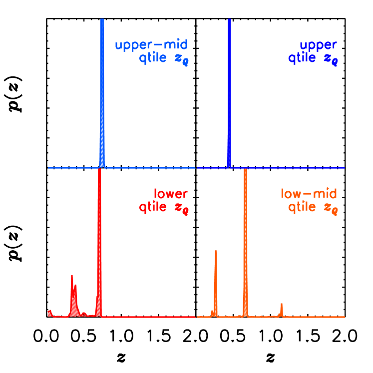
Figure 2: Random examples of redshift estimation quality in the 4 quartiles of the redshift quality parameter, $z_{Q}$ based on the $m_{814}<24~{}{\tt or}~{}S/N\geq 5$ in any optical strong line quality cut. Variation in the PDFs is noticeable.

The global contamination model for a given field is constructed in two passes. In the first, we assume that each object has a spectrum flat in units of $f_{\lambda}$ flux density with a normalisation set by its observed flux in the F814W direct image (integrated over the object’s segmentation polygon). In the second pass, we step through objects in the catalogue sorted by increasing magnitude and compute a third-order polynomial fit to each spectrum after subtracting the contamination model from any neighbours (i.e., either the flat spectra of fainter sources or the polynomial models of brighter sources). This refinement is iterated three times.

In both passes, the spatial template of the dispersed 2D model spectra is taken from the observed F814W cutout within an object’s segmentation polygon. Note that this approach neglects both morphological variation across the G800L bandpass (e.g., the PSF, continuum colour gradients, and morphological differences between line- and continuum-emitting regions). However, it provides a spatial model with much higher fidelity than any simple parametrised representation (e.g., Gaussian or Sérsic approximations).

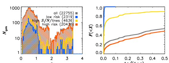
Figure 3: The redshift (left) and redshift uncertainty (right) distributions for the GLASS G800L sample. Here and in all following plots, the “high” and “low risk” samples are plotted in red and blue, respectively. These are defined based on the median $z_{Q}$ of all sources with $m_{814}<24~{}{\tt or}~{}S/N\geq 5$, whose distributions are plotted in gold. The median redshift for those sources is $\langle z\rangle\simeq 0.60$, with the low risk sample at $\langle z\rangle\simeq 0.58$. Median formal uncertainties rise from $<1\%$ for low risk to nearly 50% for high risk objects. Half of the full sample has $\Delta z/(1+z)\lesssim 0.35$. These uncertainties would be reduced by the addition of archival photometry where available, especially at $m_{814}\gtrsim 23$ (Table 1, Figure 5).

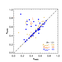
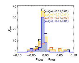
Figure 4: Top: GLASS G800L GRIZLI redshifts compared to those from VLT VIMOS as taken by various authors (see text). Agreement is quite good at $z<1$, with the global sample biased to lower redshifts by just $\Delta z=-0.01$ and with a scatter of the same order (right panel). A similar comparison with HFF photo-$z$s is presented in the Appendix.

The above process automatically yields a source and contamination model for each galaxy detected in the reference image. These can be used to “decontaminate” source spectra—i.e., remove overlapping light from neighbouring sources—to provide more accurate line and continuum characterisations. This was critical in GLASS’ crowded cluster G102 and G141 pointings, but the ACS parallels are sparse enough that source contamination is often negligible (Section 3). Note that no spectra are modelled or extracted for objects not detected in the reference frame. As such, the catalogue presented here is truncated at a F814W flux of $m_{814}=26$ with various subsamples defined by brighter flux limits (Section 3).

There are two main differences between GRIZLI and the previous GLASS pipeline. First, GRIZLI automatically handles HST grism spectra taken at one or more telescope roll angles that translate into different spectral dispersion position angles. This is implemented in that the 2D spectral models are computed in the pixel space of each separate grism exposure. This is the space in which the field-dependent grism dispersion configuration is measured and defined (e.g., Kümmel et al., 2009). This approach allows for evaluating model fits in the space of the original detector pixels with a well-calibrated noise model. Recent works have demonstrated the strengths of this approach (see Wang et al., 2018; Morishita et al., 2018a, b), though, note that the GLASS G800L data described here are observed at a single position angle. This implementation causes the ACS data format to differ from the WFC3IR data (Schmidt et al., 2014; Treu et al., 2015) in that each field’s 14 subframes are drizzle- and not interlace-combined. All weight maps account for this fact and contain the appropriate pixel-level covariances.

The second difference is that GRIZLI provides automatic redshift estimates of each source, along with its uncertainty, and “risk factor” (Tanaka et al. 2018; proportional to $1/\chi^{2}$; Section 3). This is done by evaluating fits of galaxy templates similar to those used by the EAZY code (Brammer et al., 2008). At the best redshift (typically where $\chi^{2}(z)$ is minimised but with an option to include a separate redshift prior), GRIZLI produces measurements and uncertainties of emission line fluxes and equivalent widths, as well as continuum-subtracted, 2D narrow-band maps around the emission line species. We do not use all of the GRIZLI outputs here, but they may be of value to other investigations.

Note that all of the above processing is based exclusively on the G800L spectra; no ancillary photometry is employed. This caveat should be kept in mind for analyses based solely on our catalog entries as it affects any quantity that may depend substantially on information outside the grism bandpass (e.g., stellar mass).

2.3 Products

The GLASS ACS GRIZLI reductions yield a suite of derived data products beyond the reference and spectral data frames:

1. A master FITS catalogue containing IDs and summary metrics for all extracted sources.

2. A “.beams.” FITS file containing 2D cutouts straight from each grism exposure covering a given object, and the metadata necessary for using them to generate spectral models with GRIZLI.

3. A “.stack.” FITS table for each object containing its 2D spectrum, error map, contamination and source models, and F814W direct image. All are rectified such that the spectral dispersion aligns with the data’s $x$-axis. Unlike in the .beams. files, this rectification (and drizzling) necessitates a resampling of the original detector pixels. This file’s header contains a wavelength solution, exposure time, source location, and ancillary information.

4. A “.full.” FITS table for each object containing redshift solutions, the covariance matrix and $\chi^{2}(z)$ of the template SED fits, the best-fit high-resolution template SED with and without emission lines, the rectified, drizzled F814W direct image and error map, and rectified, drizzled narrow-band images at wavelengths surrounding possible emissions lines (Section 4.2). These stamps comprise a line map, continuum estimate, contamination, and error array for each line listed in the FITS header. The header also contains a wavelength solution, exposure time, source location, line fluxes, and ancillary information.

5. A “.1D.” FITS table for each object comprising the wavelength array, contamination-subtracted source spectrum ($\rm e^{-}\,s^{-1}$), sensitivity curve [$\rm e^{-}\,s^{-1}/(erg\,s^{-1}\,cm^{-2}$ Å^-1)], RMS error ($\rm e^{-}\,s^{-1}$), and line emission and continuum models. These extractions use an optimal weighting (Horne, 1986) based on an object’s spatial profile derived from the direct image itself as described above.

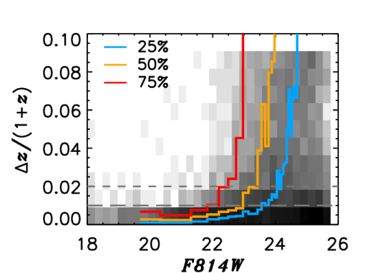
Figure 5: GLASS G800L GRIZLI redshifts are precise to $<1\%$ at $m_{814}\lesssim 22$ for most sources but degrade rapidly by $m_{814}\sim 24$, where ancillary SED coverage or strong emission lines are needed to ensure fidelity. Coloured lines show redshift uncertainty quartiles as a function of flux.

All of the above files are detailed in Appendix A, are available upon request, and will be published on GLASS’ MAST website. Useful software tools for selecting sources and matching to external catalogues will also be released (Appendix B).

3 Sample Characteristics

3.1 Counts, quality levels, and depth

GLASS’ G800L spectral database contains 22755 objects extracted to a limiting magnitude of $m_{814}=26$—roughly 1000 sources per pointing. For the purposes of this characterisation, we split these into three, somewhat overlapping, quality-based subsets defined by continuum and line $S/N$. These are:

1. All non-point sources with $m_{814}\leq 24~{}{\tt or}~{}S/N_{\rm line}\geq 5$ (“high-$S/N$+lines”; $N=4636$);

2. The subset of such galaxies below that subsample’s median GRIZLI $z_{Q}$ (“low risk”; $N=2319$);

3. Everything not in (ii) (“high risk”; $N=20436$).

Above, $S/N_{\rm line}$ refers to the $S/N$ in any of the following features as identified by GRIZLI: H$\alpha$, H$\beta$, [O ii], [O iii], [S ii], [Mg ii], or Ly$\alpha$. The magnitude cut corresponds roughly to the inferred $5\,\sigma$ continuum sensitivity—$\sim$$5\times 10^{-19}\,{\rm erg\,s^{-1}\,cm^{-2}}$ Å^-1 (Figure 1)—as measured in a $1^{\prime\prime}$ spatial aperture. “$z_{Q}$” is the GRIZLI-characterised redshift quality/risk (lower is better), which correlates well with redshift errors estimated as $\Delta z\equiv\,$84th$-$16th $P(z)$ percentile. Figure 2 shows $P(z)$ PDFs for each quartile of the $z_{Q}$ distribution.

Figure 6: F814W magnitude distributions (left) and estimated stellar mass coverage as a function of redshift (right) for the full and quality-defined samples. Color coding is as in Figure 3. Sources in the low risk sample fainter than $m_{814}=22$ tend to be high-EW line emitters. Lines therefore form the basis of redshifts in that regime, with the continuum shape playing a larger role for brighter objects. High quality sources reach $\log M_{\ast}/{\rm M}_{\odot}\sim 7$ and $\sim$9 at $z=0.60$ and 1.0, respectively, though these numbers are based on the relatively small G800L bandpass.

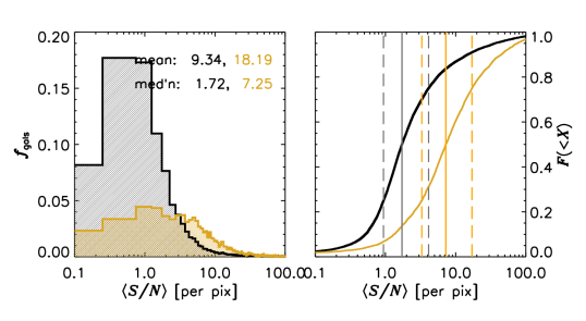
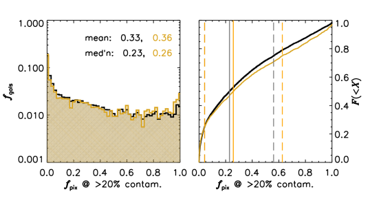
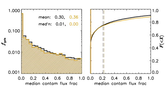
Figure 7: Top: median $S/N$ per spectral pixel from the optimal 1D extractions for all galaxies (grey) and those in the high-$S/N$+lines subsample (gold). The latter has about 3$\times$ the $S/N$ as the former. Middle: the fraction of source 2D spectral pixels whose flux is contaminated by overlapping traces to at least 20%. Unlike in the WFC3 data, fully half of G800L GLASS spectra have fewer than 20% substantially contaminated pixels. Bottom: median contaminating flux per pixel per source; another metric of contamination. Cumulative distributions for all quantities are shown at right: 75% of objects have a median per-pixel contamination of $<$20%; 75% of high-$S/N$+lines objects have typical continuum $S/N>4~{}\rm pix^{-1}$

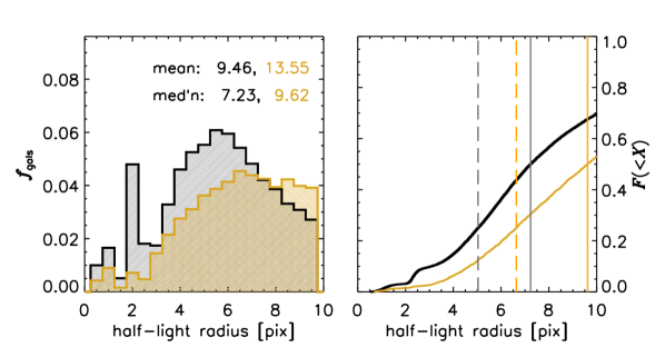
Figure 8: Sample size distribution. The high-$S/N$+lines sample comprises larger sources on average, contributing to their slightly higher contamination levels.

Figure 3 shows the sources’ inferred redshift distribution (left) and redshift error distribution (right; $\equiv\Delta z/(1+z)$). Note that, due to the inclusion of template lines spanning [O ii]$\,\lambda 3727$ and redward, there is an artifact in the redshift distribution at $z\sim 1.7$ where that feature drops out of the G800L bandpass. The sample’s median redshift is $z\simeq 0.60$, irrespective of quality cuts. Compared to the high risk subsample, the enhanced quality of the other objects’ redshifts is clear, with the $\sim$2200 low risk systems having estimates formally precise to $<$1%. Visual inspection of high quality objects suggests these redshifts are systematically accurate to within the 2 $\sigma$ formal uncertainties. The $R\sim 40$ spectral resolution makes more quantitative crosschecks difficult, but comparisons to much higher resolution VLT VIMOS spectra for 131 common objects suggest agreement is at the $\Delta z=0.01$ level with a scatter of $\sigma_{z}=0.01$ below $z=1$ (Figure 4; data from Grillo et al. 2016; Caminha et al. 2017; Karman et al. 2017; Monna et al. 2017). Figure 5 illustrates that this quality is typical at $m_{814}\lesssim 22$ ($S/N\sim 20$ per spectral pixel), and true for at least 50% of objects up to a magnitude fainter.

Figure 6, left, shows the F814W apparent magnitude distribution for the above samples. Half of the full sample is brighter than $m_{814}\approx 25$, though it is dominated by insecure redshifts at that limit. The distribution of “high-$S/N$+lines” objects cuts off sharply at $m_{814}=24$ by construction (see definition above), though counts in the low risk subsample remain relatively flat beyond this point. Comparing these histograms amplifies Figure 5’s results, suggesting that robust automated redshift estimations probably require ancillary SED information or spectral lines beyond $m_{814}\sim 22$ in these data, so catalogue values should be used cautiously. Inverted, this statement provides a selection criterion: GLASS sources fainter than that limit with tight redshifts distributions are probably high-EW line emitters.

Figure 6, right, presents the samples’ rough stellar mass ($M_{\ast}$) limit. For the low risk objects, this extends from $\log M_{\ast}/{\rm M}_{\odot}\sim 7$ at $z\sim 0.6$ to $\log M_{\ast}/{\rm M}_{\odot}\sim 9$ at $z\sim 1$—similar to the main GLASS catalogue limits (Morishita et al., 2017). We caution, however, that these estimates are based only on the information in the G800L spectrum and therefore may change significantly when ancillary photometry is included in the inference (Section 4.2).

Of course, all of the above depends fundamentally on the grism $S/N$. Figure 7, top, shows the median per-pixel $S/N$ for the full sample (grey) and the baseline quality cut ($m_{814}\leq 24$ or any line detected at $>$5 $\sigma$). In the case of the former, half of the spectra have $\langle S/N\rangle>2\,\rm pix^{-1}$, and 25% have at least twice that. The high-confidence sample has a median and upper quartile of $\sim$7 and $\sim$20, respectively, more than triple the $S/N$ of the general population. We therefore recommend basing most general analyses on at least our “high-$S/N$ + lines” quality cut, and only proceeding beyond this after more rigourous exploration of the data. Fortunately, Figure 7’s middle and bottom rows reveal that contamination is often not an impediment: half the sample has $>$50% of pixels free of any contamination. Alternatively, half of sources have $\lesssim$20% of pixels contaminated at $>$20%. Contamination (by either metric) is slightly higher for the higher quality data subset. This is likely due in part to their typically $\sim$30% larger half-light radii (Figure 8), which increases the probability of spectral collisions.

3.2 Higher level outputs: spectral line maps

The GLASS G800L catalogue contains automated spectral line identifications. Figure 9, left, shows the distribution of galaxy fractional counts as a function of the number of lines detected at $S/N_{\rm line}\geq 5$ and quality cut. The corresponding line IDs for the low risk sample are shown at right. As expected, the higher quality samples typically have 1–2 well detected lines while the general population has zero. Of detected lines, the most common are [O iii], [O ii], and the strong Balmer lines. However, even at moderate $S/N_{\rm line}$, these IDs should be treated with care: visual inspection suggests $\sim$20–40% of sources at fixed $N_{\rm lines}\in[1,3]$ may reflect spurious characterisations. Furthermore, because the line is not explicitly modelled, objects identified as [Mg ii] emitters nearly entirely reflect reduction errors or noise spikes and so should not be taken prima facie as, e.g., AGN or Lyman continuum leaker candidates (Finley et al., 2017; Henry et al., 2018). Appendix B contains example code to extract high confidence line emitters.

In addition to the total fluxes and errors for every line in every source, GRIZLI outputs 2D spectral cutouts in the relevant wavelength regions. Figure 10 shows examples of these line maps for two high-quality sources with their direct images and full 1- and 2-D spectra. The source on the left is a typical $z\sim 0.2$ starforming galaxy with prominent and extended H$\alpha$. The source on the right is a high-EW [O iii] emitter at $z\sim 0.65$ with quite different oxygen and H$\beta$ morphologies, perhaps suggesting the presence of an active galactic nucleus (though H$\beta$ is poorly resolved). We discuss these maps further in Section 4.3.

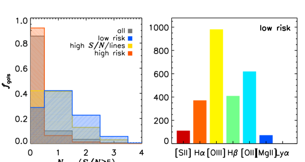
Figure 9: Line detection statistics for all galaxies and quality subsamples split as in Figure 3. Line IDs from the low risk sample cut (blue histogram at left) are shown in the right hand panel. All lines have integrated $S/N\geq 5$. Unsurprisingly, higher quality subsamples tend to have more high-confidence line detections, with the mode in the full and high-risk samples being zero lines. Of detections, the most common line is [O iii]. Note: since the line is not explicitly modelled, sources identified as [Mg ii] emitters typically reflect reduction errors or noise spikes.

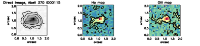
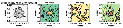
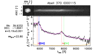
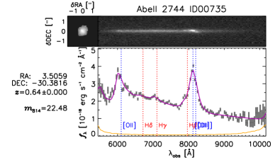
Figure 10: Top: line maps for two low risk subsample sources. Contours show 70, 80, 90% flux contours. Bottom: the sources’ direct images and 2D spectra above their 1D optimal extractions with GRIZLI model (purple) and line IDs overlaid (blue = oxygen, red = hydrogen, green = sulphur). The source on the right shows a typical redshift systematic offset for these sources. Ancillary source details are printed to the left of both spectra (coordinates, redshift, flux).

3.3 Notable sources

Slitless spectroscopy avoids the need for photometric preselection. As such, it maximises the chance of serendipitously capturing interesting sources. Figure 11 shows two of these in the GLASS G800L footprint that are also known redshift misclassifications (due to the modelling of lines only at and blueward of [O ii]$\,\lambda 3727$ in the template spectra; see Section 3.1). As revealed by its prominent Ly$\alpha$, carbon lines, and pointlike morphology, the source at left is a $z\sim 4$ quasar. Of course, GLASS data simultaneously provide a redshift survey along this QSO’s line of sight, and thus immediately suggest 61 (164) foreground candidates with a $\rho\leq 150$ (300) kpc impact parameter from the quasar suitable for characterizing H i and low-ionization species such as Mg ii (Chen et al., 2010; Prochaska et al., 2011; Rudie et al., 2012; Johnson et al., 2015). As such, this source could support higher resolution spectroscopic follow-up to learn about the circumgalactic media (CGM) of scores of galaxies (though 30-m class facilities will be needed for $R\sim 40,000$ studies). Combined with their ISM maps (Figure 10), the CGM enrichment levels/temperatures/ionization states derived from such follow-up could provide powerful empirical constraints on metal transport, and therefore evolutionary models (e.g., Davé et al., 2011, 2017; Peeples et al., 2014; Muratov et al., 2015). Both of these studies are enabled by slitless spectroscopy.

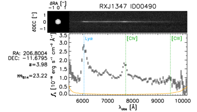
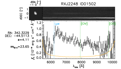
Figure 11: Examples of two known redshift misclassifications. Both the QSO (left) and LBG (right) are at $z\sim 4$ but were initially placed at $z=0.89$ and $z=0.70$, respectively. More examples of the $\sim$300 bright, $S/N\geq 5$ [O iii] emitters in the GLASS G800L database are shown in Appendix D.

Figure 11, right, shows another $z\sim 4$ source. As opposed to the QSO, this object’s lack of Ly$\alpha$ emission, strong Ly$\alpha$ break, and extended morphology reveal it to be a Lyman Break Galaxy (LBG). Large samples of such objects at these redshifts exist (e.g., Bouwens et al., 2015), but spectroscopy remains difficult. The low backgrounds in space and avoidance of slit losses, however, make HST efficient at spectroscopically identifying LBGs. Indeed, at $m_{814}=23.8$, this object shows that GLASS’ data reach continuum levels comparable to those from surveys on 10-m class ground-based telescopes for similar integration times (albeit at lower spectral resolution; Steidel et al., 1999; Shapley et al., 2003).

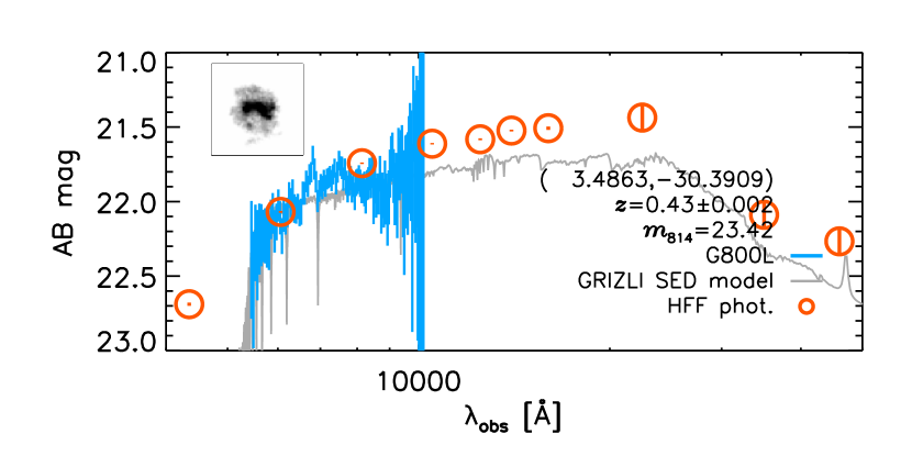
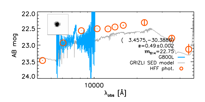
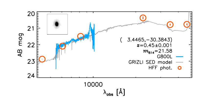
Figure 12: Examples of GLASS G800L spectra (blue) and GRIZLI-inferred continuum SEDs (grey) shown with matched source photometry from the HFF campaign (Shipley et al., 2018, orange circles). Some inferences agree remarkably well with photometry lying well outside the grism bandpass despite its limited coverage; others are less consistent. Such offsets—typically at the $\sim$0.25 mag level (Section 4.2)—will affect stellar mass and SFR estimates. However, the consistent location of observed and inferred features (e.g., the 1.6 µm bump) support the accuracy of these sources’ grism-determined redshifts (see also Figure 14). These data are available to anyone wishing to perform joint spectrophotometric SED fitting on the the 13 fields where HST photometry exist (Table 1). More examples of low risk objects in the HFF footprints are shown in Appendix D.

4 Discussion and Further Applications

The GLASS G800L database will support a range of investigations. We note three potentially fruitful avenues below beyond the QSO and LBG follow-up studies just discussed.

4.1 Infalling cluster members

As shown in Table 1, each pointing in the catalogue contains $\sim$20–40 objects within $2000~{}{\rm km}\,\rm s^{-1}$ of the HFF or CLASH cluster redshifts. These are likely galaxies either falling into the cluster potential for the first time, or “splashing back” after one or more crossings through the clusters (More et al., 2015; Baxter et al., 2017). Both cases present opportunities to study the forces affecting galaxies in the densest environments in the Universe. We encourage anyone interested in ram pressure stripping (Gunn & Gott, 1972) or preprocessing (Zabludoff & Mulchaey, 1998) to explore these objects. Analogous analyses to Vulcani et al. (2015, 2016, 2017, see Section 4.3) but based on [O iii] may, for example, prove powerful.

4.2 Joint analyses with HST photometry

Over half of the sources in the database lie in regions covered by CLASH, HFF, or other HST imaging. Given the limited bandpass of the G800L grism, incorporating these data into any further SED fitting is valuable, especially for analyses that rely on accurate stellar mass or SFR inferences. Figure 12 shows the GLASS spectra overlaid on HFF photometry for three of the 859 common GLASS/Shipley et al. (2018) sources in the Abell 2744 parallel field. For low risk sources, the relative fluxing between the grism data and HFF photometry is good to $\Delta m_{814}=0.1$ mag (such that HFF fluxes are brighter) with a scatter of 0.25 mag about that offset. The grism-derived continuum SED model extrapolated well outside the G800L bandpass can be predictive to similar levels—low risk median $m_{{\tt GRIZLI}}-m_{\rm HFF}=[0.19,0.25,0.25,0.25]$ in [F105,125,140,160W] with $>$0.5 mag scatters around these offsets—but larger disagreements in the IR and UV can obviously occur.

Moreover, the combination of low resolution grism spectroscopy covering, e.g., the Balmer or 4000 Å breaks with broadband photometry to the red and blue is now being used to great effect in inferring the star formation histories (SFHs) of galaxies at $0.3<z<3$, not just observed quantities (Dressler et al., 2016; Dressler et al., 2018; Abramson et al., 2018; Morishita et al., 2018b). Figure 12 shows the GLASS data will support similar analyses at $z\sim 0.4$–1.25, and Figure 13 shows an example estimate (L. Abramson, in preparation). Critically, given their high spatial resolution and low contamination, these data could support spatially resolved SED analyses to constrain individual galaxies’ joint mass and structural evolution over at least the past $\sim$1–2 Gyr. These empirical inferences can be compared to simulations to provide direct, longitudinal tests of numerical physical prescriptions, not just bulk predictions for the galaxy population at large. Abramson et al. (2018) performed such an analysis, but were limited to just 4 systems due to the high contamination rates in GLASS’ central WFC3 pointings. The G800L data do not suffer from this issue, so spatially resolved spectrophotometric SFH reconstructions based on functional [e.g., by pyspecfit (Newman et al., 2014), or other means (Iyer & Gawiser, 2017)] or free-form inferential techniques (Pacifici et al., 2012; Kelson et al., 2014; Leja et al., 2017; Morishita et al., 2018b) should yield a valuable database of hundreds of high quality mass, SFR, and structural histories over large ranges in observed mass, SFR, and structural parameters.

Figure 13: Left: a GLASS G800L spectrum of a starforming galaxy at $z=0.44$ (grey bars showing 1 $\sigma$ errors) with HFF + Spitzer photometry from Shipley et al. (2018) (white circles). The maximum likelihood Bruzual & Charlot (2003) SED fit is overlaid in blue (photometry in diamonds) with the 5%, 50%, and 95% probability fits in orange. The inferred contribution from emission lines is plotted in cyan at bottom. Middle: the SFH (${\rm SFR}(t)$) inferred from this SED using a library of 3000 $H=1$ stochastic model SFHs from Kelson (2014). The blue line is the maximum likelihood output, with the rust- and mustard-coloured bands showing the 95% and 68% confidence envelopes, respectively, and the median plotted in orange. The inset shows the fractional mass growth history (same intervals) with the 95% envelope from the prior plotted in hatched white lines. Right: the inferred absolute mass growth history with $M_{\ast}$, $Z_{*}$, and $A_{V}$ covariances plotted in the inset. According to this fit—which marginalises over the choice of a Reddy, Calzetti, SMC, and Milky Way dust law—this galaxy has an observed $\log M_{\ast}/{\rm M}_{\odot}=9.3\pm 0.06$ (Chabrier 2003 IMF) with a half-mass redshift of $z\simeq 0.8$ and has grown in a relatively linear fashion for at least $0.5\,t_{\rm Hubble}$. The machinery that performed this fit will be described in a future paper (L. Abramson, in preparation), but is similar to that described by Pacifici et al. (2012). The GLASS G800L data combined with extant photometry will support analyses of SFHs derived using these and other tools.

4.3 Emission line mapping

As mentioned in Sections 1, 3.2, Figure 10 illustrates one of the key advantages of HST and future space-based slitless spectroscopy: the automatic production of spatially resolved spectral features mapped at the diffraction limit—600 pc at $z=0.6$ (${\rm FWHM}=0\aas@@fstack{\prime\prime}09$). These maps can be used, for example, to infer galaxy metallicity distributions and even outflow patterns at sub-kpc scales to challenge numerical feedback and star formation models in new ways. For example, Vulcani et al. (2015, 2016, 2017) used the G102 H$\alpha$ maps from GLASS’ central pointings to study the connection between galaxy stellar and gas morphology, and associate this with various features of the local and global environment in clusters. Jones et al. (2015) and Wang et al. (2017) used oxygen and H$\beta$ to produce gas-phase metallicity maps and gradients for sources at $z\sim 1$–3 and unprecedentedly low stellar masses ($\log M_{\ast}\lesssim 8$). Wang et al. (2018) identified two such sources with steeply positive gradients ($[{\rm O/H}]\propto r$) and used simple models to produce outflow maps and mass loading factors as a function of underlying stellar mass density, showing that individual systems are not described well by only energy or momentum driven wind models. The GLASS G800L data will support similar studies based on [O ii] through H$\alpha$ lines at $z\lesssim 1$, both outside and in the infall regions around massive clusters. Further two-dimensional explorations of the ISM will no doubt be fruitful.

5 Summary

We present a catalogue of 22755 objects with ACS G800L slitless spectroscopy from the 20 GLASS parallel fields (Table 1). The catalogue extends to $m_{814}=26$ with uniform 7-orbit ($\sim$10 ks) coverage over $\sim$220 sq. arcmin. Sources have a median redshift of $z=0.60$ with median uncertainties of $\Delta z/(1+z)\lesssim 0.02$ at $m_{814}\leq 23$ (Figures 3, 5) and are typically contaminated at the 0%–20% level (Figure 7). About a quarter of the sample either has continuum flux detected at $\geq$5 $\sigma$ ($m_{814}\lesssim 24;~{}f_{\lambda}\approx 5\times 10^{-19}~{}{\rm erg~{}s^{-1}~{}cm^{-2}~{}\AA^{-1}}$) or $S/N>5$ in at least one spectral line ($f_{\rm lim}\approx 5\times 10^{-17}~{}{\rm erg~{}s^{-1}~{}cm^{-2}}$) such that median redshift errors are $<$1%. Incorporating photometry for the 13 fields that overlap with extant HST imaging from CLASH, HFF, or other programs will allow redshifts to be obtained to much greater depth and support a rich variety of spectrophotometric studies into galaxy star formation histories at $z\sim 0.5$–1.5 (Section 4.2).

The full catalogue also contains full 2D spectra, contamination, and source models for each object, along with automated line identifications, fluxes, uncertainties, and 2D spatially resolved maps produced by GRIZLI. Optimal 1D extractions are also provided, as are full UV–sub-mm best-fit SEDs and redshift PDFs. All data and derived products are available on request, and will be published on MAST along with code for performing various basic operations—which we also give here in Appendix B.

These data and products will support a wide range of investigations—from mapping galaxy outflows at $z<0.8$ (Sections 3.2, 4.3) to identifying QSOs and LBGs at $z\sim 4$ (Section 3.3)—and serve as useful intuition-builders as the field prepares for the increasing ubiquity of slitless spectroscopy in the eras of JWST and WFIRST.

Facilities: HST ACS.

Software: IDL (Coyote libraries; http://www.idlcoyote.com/), python (GRIZLI).

Appendix A File Names, Formats, and Contents

The core component of the GLASS G800L database is the catalogue master FITS table:

1. glass-acs-2019.05.10.fits.

This table contains field names and IDs for all extracted sources—from which their data filenames can be constructed—along with a wealth of summary metrics described at the end of this Appendix.

The master FITS file is designed for the database’s organization into 20 folders—one for each ACS pointing. These are named by their field centroid coordinates in the format:

1. jRARA${}^{\rm p}_{\rm m}$DEDE,

such that ‘j0014m3023’ corresponds to the Abell 2744 parallel at PA 323. These correspond to the ROOT column in the master catalogue. Within each folder, all objects are identified by a source number, corresponding to the ID column. As such, the master catalogue can be used to point to the ii-th object’s datafiles by writing:

⬇

folder = mastercat[ii].ROOT

sourceID = string(mastercat[ii].ID, f = ’(FI05)’)

sourceFileBase = folder+’/’+folder+’_’+sourceID

which will construct the base filename from which a source’s data files are built (Appendix B).

A.1 Individual source files

As mentioned in Section 3, each source is associated with three files. These are defined by the following suffixes appended to their base ID jRARA${}^{\rm p}_{\rm m}$DEDE_0IDID:

1. “.stack.fits” – A 9 layer 2D FITS table containing:

   1. SCI – A source’s rectified, drizzled 2D spectral cutout;

   2. WHT – inverse variance array;

   3. CONTAM – contamination model;

   4. MODEL – source model;

   5. KERNEL – F814W direct image used to convolve the 2D trace to a common spatial sampling.

   Layers 1, 2, 4, and 5 are then repeated with the source resampled to a common PA. Since each GLASS source is observed only once, this PA is set to the PA of observation, such that the layers are identical (to $<$1%). This file’s header also contains the wavelength solution, exposure time, RA/DEC, and other ancillary information.

2. “.full.fits” – An $N\geq 5$ layer 2D FITS table containing:

   1. ZFIT_STACK – A 6-column table containing redshift estimation information. This includes the ZGRID redshift array, $P(z)$ distribution (PDF), redshift RISK and CHI2 goodness of fit distributions, and SED template/redshift covariance matrix (COVAR);

   2. COVAR – Covariance matrix of the template fit coefficients at the best-fit redshift (taken to be where $P(z)$ is maximised from the previous extension).

   3. TEMPL – A 3-column table containing the best fit SED (FULL), continuum-only model (CONTINUUM), and wavelength array spanning $0.02<\lambda/\micron<2\times 10^{4}$ (WAVE);

   4. DSCI – F814W source direct image;

   5. DWHT – F814W image weight map;

   6. LINE001 – Map of LINE001 in the file header;

   7. CONTINUUM – Continuum near LINE001 in the file header;

   8. CONTAM – Contamination near LINE001 in the file header;

   9. LINEWHT – Weight map near LINE001 in the file header;

   10. LINE002 – As above, but for LINE002 in the file header;

   Layers 6–$N$ will not be present in an object with no entries in the master catalogue’s HASLINES column (see below) or no lines in this file’s header. Otherwise, e.g., H$\alpha\beta\gamma\delta$, [O ii] and [O iii], [S ii] have names “Ha, Hb, Hg, Hd, OII, OIII, SII,” etc. There is one set of 4 layers for each line. The header also contains the wavelength solution, exposure time, RA/DEC, line fluxes, and other ancillary information.

3. “.1D.fits” – A 6 column 1D FITS table containing:

   1. WAVE – Wavelength array spanning only the G800L bandpass ($5450<\lambda/$Å $<10170$);

   2. FLUX – Optimally extracted, contamination subtracted 1D source spectrum ($\rm e^{-}\,s^{-1}$);

   3. ERR – 1 $\sigma$ noise on FLUX ($\rm e^{-}\,s^{-1}$);

   4. FLAT – Sensitivity curve needed to transform the above into $f_{\lambda}$ ($\rm e^{-}\,s^{-1}/erg\,s^{-1}\,cm^{-2}\,\AA^{-1}$);

   5. LINE – Best fit galaxy SED template, including emission lines.

   6. CONT – Best fit galaxy SED template, continuum only.

The getfname function in Appendix B will return the filenames for all of the above FITS tables given a source’s ROOT and ID entry in the GLASS master catalogue.

A.2 Master catalogue column definitions

The following entries are found in the GLASS G800L master catalogue FITS table:

• ROOT – ACS field (string)

• ID – Source ID in ROOT (int)

• RA – Source RA (J2000, decimal deg.; double)

• DEC – Source DEC (J2000, decimal deg.; double)

• NINPUT – $N$ frames in source’s G800L coadd (int; 1 –14)

• REDSHIFT – Source redshift estimate ($=z_{\rm MAP}$; float)

• NUMLINES – Number of potential lines in source spectrum (int; 0 –10)

• HASLINES – Emission line IDs (string; space-separated)

• CHI2POLY – $\chi^{2}$ of a third-order polynomial fit to the spectrum (float)

• DOF – Approximate spectral degrees of freedom given by the total number of unmasked pixels in the “beams” spectra extracted from the grism exposures (float)

• CHIMIN – Minimum $\chi^{2}$ of the SED template fit on a redshift grid (float)

• CHIMAX – Maximum $\chi^{2}$ of the SED template fit on a redshift grid (float)

• BIC_POLY – “Bayesian Information Criterion” of the polynomial fit; $\ln(\mathtt{DOF})\cdot k+(\mathtt{CHI2POLY-CHIMIN})$, where $k=4+N_{b}$ and $N_{b}$ the number of spectra in the .beams. file, since an additive background component is fit for each.

• BIC_TEMP – Bayesian Information Criterion of the template fit, where $k=N_{c}+N_{b}$ and $N_{c}$ is the number of non-zero template fit coefficients.

• BIC_DIFF – Difference $\mathtt{BIC\_POLY}-\mathtt{BIC\_TEMP}$. Large values generally correspond to cases where the galaxy SED templates much better explain the observed spectrum than the trivial polynomial fit.

• Z02 – 2 $\sigma$ redshift lower limit (float)

• Z16 – 1 $\sigma$ redshift lower limit (float)

• Z50 – 50% confidence redshift estimate (float)

• Z84 – 1 $\sigma$ redshift upper limit (float)

• Z97 – 2 $\sigma$ redshift upper limit (float)

• ZWIDTH1 – 1 $\sigma$ $\Delta z$ ($84-16$; float)

• ZWIDTH2 – 2 $\sigma$ $\Delta z$ ($97-2$; float)

• Z_MAP – Maximum likelihood redshift (same as REDSHIFT; float)

• Z_RISK – Redshift where the “risk” is minimised, where risk is defined as in Tanaka et al. (2018) (float)

• MIN_RISK – Risk estimate at Z_RISK (float)

• FLUX_{LINE} – Line flux (erg sec^-1 cm^-2 Å^-1; float)

• ERR_{LINE} – Line error (erg sec^-1 cm^-2 Å^-1; float)

• EW50_{LINE} – Median line equivalent width drawn from the line-plus-continuum covariance matrix (observed-frame Å; float)

• EWHW_{LINE} – Half-width between the 16 and 84th percentiles of the EW estimates for a given line (observed-frame Å; float)

• SN_{LINE} – Line $S/N=\tt FLUX/ERR$ (float)

• CHINU – Spectral model fit reduced $\chi^{2}$ ($\tt CHIMIN/DOF$; float)

• ZQ – EAZY redshift risk assessment (float)

• IDX – Vizier search query URL for this source (string)

• ELLIPTICITY – SExtractor ELLIPTICITY measure (float)

• MAG_AUTO – SExtractor MAG_AUTO (F814W; float)

• FLUX_RADIUS – SExtractor half-light radius (F814W pix; float)

• A_IMAGE – SExtractor semimajor axis length (F814W pix; float)

• T_G800L – Total G800L exposure time (seconds; float)

• IS_POINT – Point source flag (bit)

where “{LINE}” refers to each of the following:

• He i $\lambda 1083$, He ii $\lambda 1640$;

• Lyman $\alpha$;

• N v $\lambda 1240$, N iv $\lambda 1487$, N iii] $\lambda 1750$;

• C iv $\lambda 1549$, C iii] $\lambda 1908$;

• [O iii] $\lambda 1663$, [O ii] $\lambda 3727$, [O iii] $\lambda 4363$, [O iii] $\lambda\lambda 4959,5007$, [O i] $\lambda 6302$;

• [Mg ii];

• [Ne v] $\lambda 3346$, [Ne vi] $\lambda 3426$, [Ne iii] $\lambda 3867$;

• H$\delta$, H$\gamma$, H$\beta$, H$\alpha$+[N ii];

• [S ii] $\lambda\lambda 6716,6731$, [S iii] $\lambda\lambda 9069,9532$.

Various quantities inferred from the template SED fits ($M/L$, $M_{\ast}$, sSFR, and implied fluxes in various filters) are also given, but—as noted in the main text—these estimates are not typically reliable and so caution against their use (Section 3.1).

Appendix B Useful Algorithms

Below are some useful IDL routines to perform some basic data operations mentioned in the main text.

B.1 Return the high $S/N$+lines and low/high risk subsamples:

⬇

function getGoldSample, mastercat, $

MAGLIM = maglim, $

SNLIM = snlim

if NOT keyword_set(MAGLIM) then maglim = 24.

if NOT keyword_set(SNLIM) then snlim = 5.

;; Define ‘high S/N + lines’ objects

hiQ = where(mastercat.MAG_AUTO le maglim OR $

(mastercat.SN_HA ge snlim OR $

mastercat.SN_HB ge snlim OR $

mastercat.SN_OII ge snlim OR $

mastercat.SN_OIII ge snlim OR $

mastercat.SN_SII ge snlim OR $

mastercat.SN_MGII ge snlim OR $

mastercat.SN_LYA ge snlim) AND NOT $

mastercat.IS_POINT, compl = nhiQ)

;; Use highQ to define ‘low’ and ‘high risk’

;; after nulling the not-hiQ qualities

mastercat[nhiQ].ZQ = 0

medrisk = median(mastercat[highQ].ZQ)

loRisk = where(mastercat.ZQ le medrisk, $

compl = hiRisk)

indices = {HIQ: hiQ, NOTHIQ: nhiQ, $

LORISK: loRisk, HIRISK: hiRisk}

RETURN, indices

end

B.2 Match to HFF photometry from Shipley et al. (2018):

⬇

function loadHffPhot, hffPhotFile

;; Restore the Shipley et al. .save catlaog

restore, hffPhotFile

ninds = n_elements(ra)

;; Find the NIR intrument

if n_elements(f_KS_HAWKI) gt 0 then begin

fks = f_KS_HAWKI

eks = e_KS_HAWKI

flgks = redflag_KS_HAWKI

endif else begin

fks = f_KS_MOSFIRE

eks = e_KS_MOSFIRE

flgks = redflag_KS_MOSFIRE

endelse

;; Create the SED, error, and flag arrays

;; (F435W--Spitzer 4.5 um)

fluxes = transpose([[f_F435W], [f_F606W], [f_F814W], [f_F105W], [f_F125W], [f_F140W], [f_F160W], [fks], [f_CH1], [f_CH2]])

errs = transpose([[e_F435W], [e_F606W], [e_F814W], [e_F105W], [e_F125W], [e_F140W], [e_F160W], [eks], [e_CH1], [e_CH2]])

flags = transpose([[redflag_F435W], [redflag_F606W], [redflag_F814W], [redflag_F105W], [redflag_F125W], [redflag_F140W], [redflag_F160W], [flgks], [redflag_CH1], [redflag_CH2]])

;; Add the MW dust and zeropoint corrections

;; (should they be necessary; key names differ

;; slightly between catalogues)

mwcorr = transpose([[mw_F435W], [mw_F606W], [mw_F814W], [mw_F105W], [mw_F125W], [mw_F140W], [mw_F160W], [1.0], [1.0], [1.0]])

if N_ELEMENTS(zpcorr_f814w) gt 0 then $

zpcor = transpose([[zpcorr_F435W], [zpcorr_F606W], [zpcorr_F814W], [zpcorr_F105W], [zpcorr_F125W], [zpcorr_F140W], [zpcorr_F160W], [1.0], [1.0], [1.0]]) $

else $

zpcor = transpose([[zpcor_F435W], [zpcor_F606W], [zpcor_F814W], [zpcor_F105W], [zpcor_F125W], [zpcor_F140W], [zpcor_F160W], [1.0], [1.0], [1.0]])

;; Set up the output

nbands = n_elements(fluxes[*,0])

results = {LAMBDA: [4350., 6060., 8140., $

10500., 12500., 14000., 16000., $

22500., 35000., 46000.], $

SED : fltarr(nbands), $

ESED : fltarr(nbands), $

FLAGS: bytarr(nbands), $

RA : 0.d, $

DEC : 0.d, $

MWCORR: fltarr(nbands), $

ZPCORR: fltarr(nbands)}

results = replicate(results, ninds)

;; Fill the output structure

;; get fluxes to erg/s/cm2/Hz

ninds = n_elements(ra)

for ii = 0, ninds - 1 do begin

results[ii].SED = fluxes[*,ii]/10.^29.44

results[ii].ESED = errs[*,ii]/10.^29.44

results[ii].FLAGS = flags[*,ii]

results[ii].RA = ra[ii]

results[ii].DEC = dec[ii]

results[ii].MWCORR = mwcorr

results[ii].ZPCORR = zpcor

endfor

RETURN, results

end

;;

;;

;;

pro getSpecPhot, mastercat, field

if field ne ’Abell 2744’ AND $

field ne ’MACS0717’ AND $

field ne ’MACS1149’ AND $

field ne ’RXJ2248’ then $

print, ’NO HFF ANCILLARY PHOTOMETRY AVAILABLE’ $

else begin

;; Load spectral database

data = mrdfits(mastercat, 1)

;; Load photometry

phot = loadhffphot(field)

;; Match with a 1’’ radius

spherematch, phot.RA, phot.DEC, $

data.RA, data.DEC, 1./3600, $

minds, sinds, len

;; Trim and align databases

data = data[sinds]

phot = phot[minds]

endelse

... ;; Operations go here

end

B.3 Get sources emitting $N_{\rm lines}$ lines at high confidence:

⬇

function getHighSnLines, mastercat, $

SNCUT = sncut

if NOT keyword_set(SNCUT) then sncut = 5.

;; Set up the output storage

;; allowing for up to 10 high-sn lines

output = {NUMLINES: 0, $

IDS: strarr(10), $

SNS: fltarr(10)}

output = replicate(output, n_elements(mastercat))

;; Go through the lines and get their S/N

for ii = 0, n_elements(mastercat) - 1 do begin

lines = mastercat[ii].HASLINES

lines = strsplit(lines, ’ ’, /extr)

if mastercat[ii].NUMLINES gt 0 then begin

tsn = fltarr(mastercat[ii].NUMLINES)

for jj = 0, mastercat[ii].NUMLINES - 1 do begin

tl = lines[jj]

case tl of

’Ha’: tsn[jj] = mastercat[ii].SN_HA

’Hb’: tsn[jj] = mastercat[ii].SN_HB

’OII’: tsn[jj] = mastercat[ii].SN_OII

’OIII’: tsn[jj] = mastercat[ii].SN_OIII

’SII’: tsn[jj] = mastercat[ii].SN_SII

’MgII’: tsn[jj] = mastercat[ii].SN_MGII

’Lya’: tsn[jj] = mastercat[ii].SN_LYA

... ;; More line names here.

endcase

endfor

;; Count and store lines about S/N threshold

foo = where(tsn ge sncut, nlines)

output[ii].NUMLINES = nlines

if nlines gt 0 then begin

output[ii].IDS[0:nlines-1] = lines[foo]

output[ii].SNS[0:nlines-1] = tsn[foo]

endif

endif

endfor

RETURN, answer

end

B.4 Get all of the data file names for a given source:

⬇

function getfname, root, id

fname = root+’/’+root+’_’+string(id, f = ’(I05)’)+’.XXX.fits’

stack = repstr(fname, ’XXX’, ’stack’)

full = repstr(fname, ’XXX’, ’full’)

oneD = repstr(fname, ’XXX’, ’1D’)

srcName = root+’_’+string(id, f = ’(I05)’)

fnames = {ONED: oneD, $

FULL: full, $

STACK: stack, $

SRCNAME: srcName}

RETURN, fnames

end

Appendix C Comparison to Extant Photometric Redshifts

Shipley et al. (2018) provides photometric redshifts for GLASS G800L sources in the HFF footprint. Figure 14 compares these to the grism-only redshifts. Agreement is quite good for low risk sources, and unbiased for the full high-$S/N$+lines sample. The low risk sample is consistent with gaussian errors, though errors may be slightly underestimated for the other samples ($\sigma/\sqrt{2}\langle{\rm err}\rangle>1$). Nevertheless, this analysis supports our conclusion that the $\sim$2200 low risk objects should be immediately useful to analyses “straight out of the box.”

Appendix D Further Data Examples

Below are more examples of GLASS G800L spectra and combined spectrophotometry for select sources in the HFF footprint. All galaxies shown Figure 15 have $S/N_{\rm[OIII]}\geq 5$ and are above the median brightness in the low risk sample. There are 304 such sources in the GLASS ACS database. All galaxies in Figure 16 are in the low risk sample with matching HFF photometry. There are 383 such objects in the GLASS ACS database (3411 in total with HFF overlap).

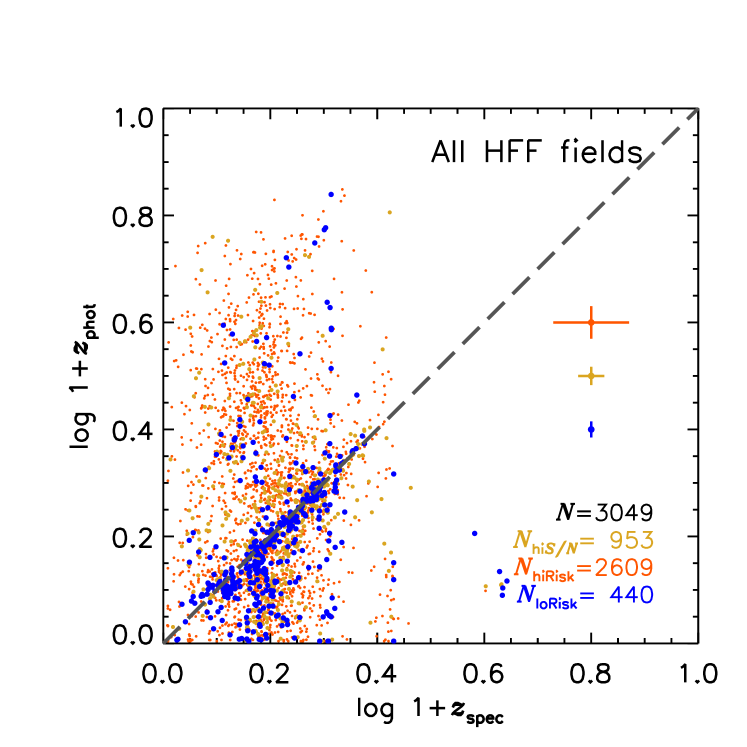
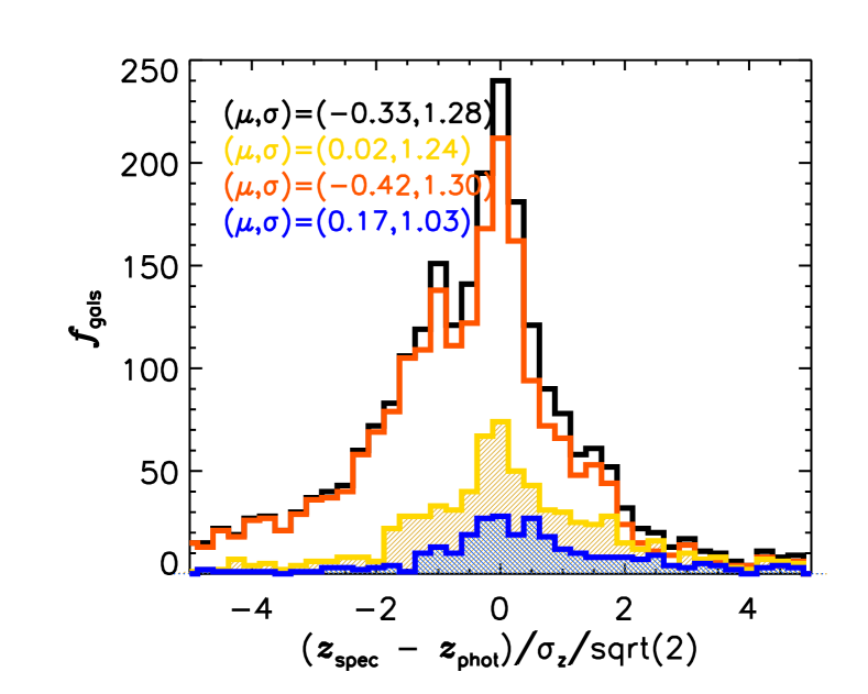
Figure 14: Similar to Figure 4 but plotting HFF photometric redshifts from Shipley et al. (2018) ($z_{\rm phot}$) against GLASS G800L redshifts ($z_{\rm spec}$). Distributions are much wider, but agreement is still fair, with low risk sources having photo-$z$ errors consistent with gaussian noise. All samples show slight biases, but those for high-$S/N$+lines and low-risk sources are small in the mean.

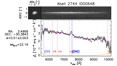
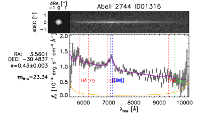
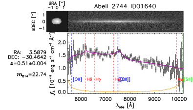
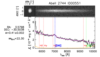
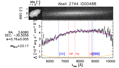
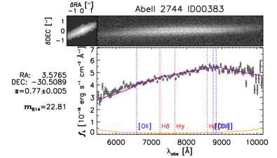
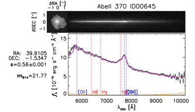
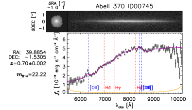
Figure 15: Examples of the $\sim$300 bright, $S/N\geq 5$ [O iii] emitters in the glass database. This figure continues on the following page.

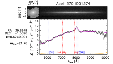
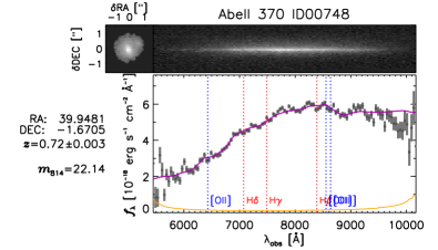
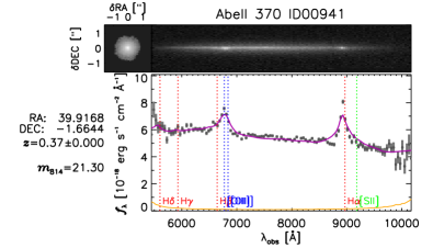
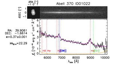
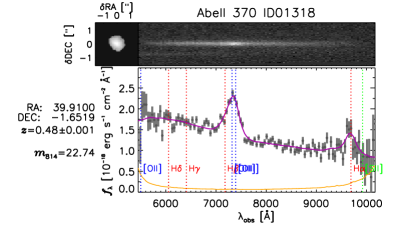
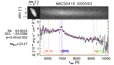
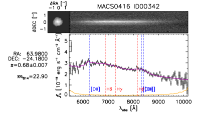
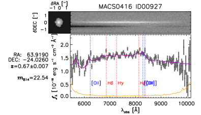
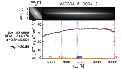
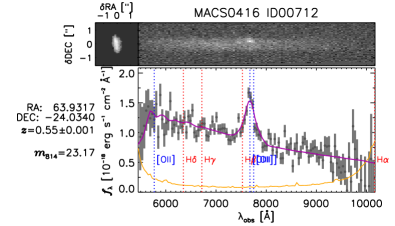
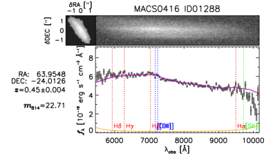
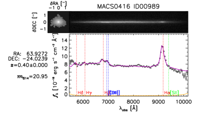
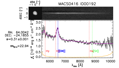
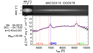
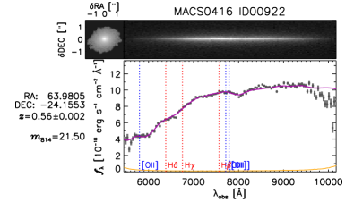
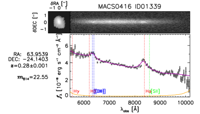
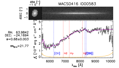
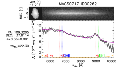
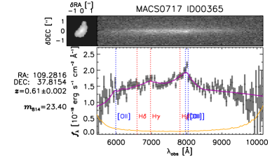
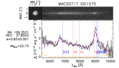
Figure 15: Examples of the $\sim$300 bright, $S/N\geq 5$ [O iii] emitters in the glass database. This figure continues on the following page. This figure continues on the following page.

Figure 15: Examples of the $\sim$300 bright, $S/N\geq 5$ [O iii] emitters in the glass database. This figure continues on the following page.

Figure 15: Examples of the $\sim$300 bright, $S/N\geq 5$ [O iii] emitters in the glass database.

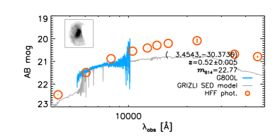
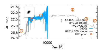
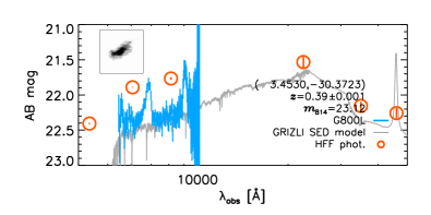
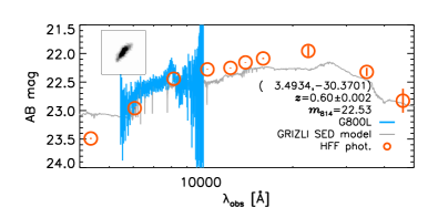
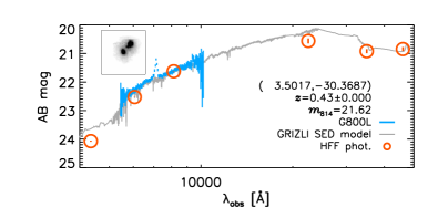
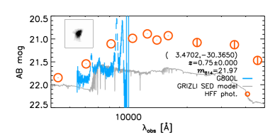
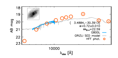
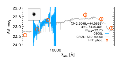
Figure 16: GLASS G800L sources in the Abell 2744 and RXJ2248 parallel fields matched to HFF photometry from Shipley et al. (2018). This figure is continued on the following page.

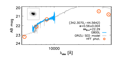
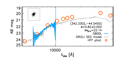
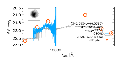
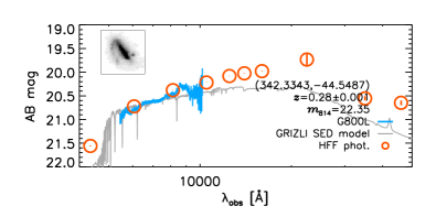
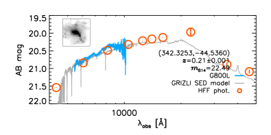
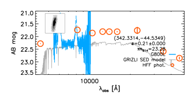
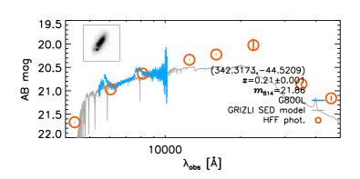
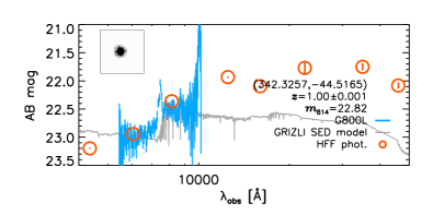
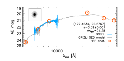
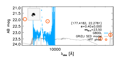
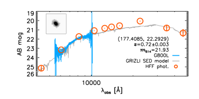
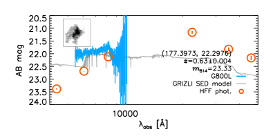
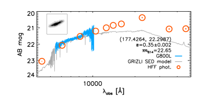
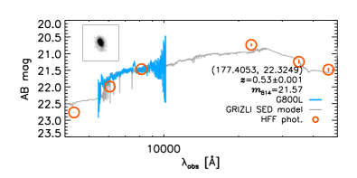
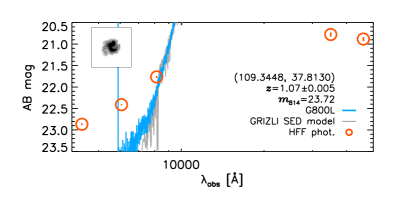
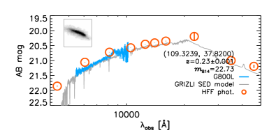
Figure 16: GLASS G800L sources in the Abell 2744 and RXJ2248 parallel fields matched to HFF photometry from Shipley et al. (2018). This figure is continued on the following page.

Figure 16: GLASS G800L sources in the MACS0717 and MACS1149 parallel fields matched to HFF photometry from Shipley et al. (2018).

References

- Abramson et al. (2018) Abramson L. E., et al., 2018, AJ, 156, 29
- Baxter et al. (2017) Baxter E., et al., 2017, ApJ, 841, 18
- Bertin & Arnouts (1996) Bertin E., Arnouts S., 1996, A&AS, 117, 393
- Bouwens et al. (2015) Bouwens R. J., et al., 2015, ApJ, 803, 34
- Brammer et al. (2008) Brammer G. B., van Dokkum P. G., Coppi P., 2008, ApJ, 686, 1503
- Brammer et al. (2012) Brammer G. B., et al., 2012, ApJS, 200, 13
- Bruzual & Charlot (2003) Bruzual G., Charlot S., 2003, MNRAS, 344, 1000
- Caminha et al. (2017) Caminha G. B., et al., 2017, A&A, 600, A90
- Chabrier (2003) Chabrier G., 2003, PASP, 115, 763
- Chen et al. (2010) Chen H.-W., Helsby J. E., Gauthier J.-R., Shectman S. A., Thompson I. B., Tinker J. L., 2010, ApJ, 714, 1521
- Davé et al. (2011) Davé R., Finlator K., Oppenheimer B. D., 2011, MNRAS, 416, 1354
- Davé et al. (2017) Davé R., Rafieferantsoa M. H., Thompson R. J., Hopkins P. F., 2017, MNRAS, 467, 115
- Dressler et al. (2016) Dressler A., et al., 2016, ApJ, 833, 251
- Dressler et al. (2018) Dressler A., Kelson D. D., Abramson L. E., 2018, ApJ, 869, 152
- Finley et al. (2017) Finley H., et al., 2017, A&A, 608, A7
- Gaia Collaboration et al. (2018) Gaia Collaboration et al., 2018, A&A, 616, A14
- Gonzaga & et al. (2012) Gonzaga S., et al. 2012, The DrizzlePac Handbook
- Grillo et al. (2016) Grillo C., et al., 2016, ApJ, 822, 78
- Gunn & Gott (1972) Gunn J. E., Gott III J. R., 1972, ApJ, 176, 1
- Henry et al. (2018) Henry A., Berg D. A., Scarlata C., Verhamme A., Erb D., 2018, ApJ, 855, 96
- Horne (1986) Horne K., 1986, PASP, 98, 609
- Iyer & Gawiser (2017) Iyer K., Gawiser E., 2017, ApJ, 838, 127
- Johnson et al. (2015) Johnson S. D., Chen H.-W., Mulchaey J. S., 2015, MNRAS, 449, 3263
- Jones et al. (2015) Jones T., et al., 2015, AJ, 149, 107
- Karman et al. (2017) Karman W., et al., 2017, A&A, 599, A28
- Kelson (2014) Kelson D. D., 2014, preprint, (arXiv:1406.5191)
- Kelson et al. (2014) Kelson D. D., et al., 2014, ApJ, 783, 110
- Kriek et al. (2015) Kriek M., et al., 2015, ApJS, 218, 15
- Kümmel et al. (2009) Kümmel M., Walsh J. R., Pirzkal N., Kuntschner H., Pasquali A., 2009, PASP, 121, 59
- Kümmel et al. (2011) Kümmel M., et al., 2011, A&A, 530, A86
- Leja et al. (2017) Leja J., Johnson B. D., Conroy C., van Dokkum P. G., Byler N., 2017, ApJ, 837, 170
- Lotz et al. (2017) Lotz J. M., et al., 2017, ApJ, 837, 97
- Momcheva et al. (2016) Momcheva I. G., et al., 2016, ApJS, 225, 27
- Monna et al. (2017) Monna A., et al., 2017, MNRAS, 466, 4094
- More et al. (2015) More S., Diemer B., Kravtsov A. V., 2015, ApJ, 810, 36
- Morishita et al. (2017) Morishita T., et al., 2017, ApJ, 835, 254
- Morishita et al. (2018a) Morishita T., et al., 2018a, arXiv e-prints,
- Morishita et al. (2018b) Morishita T., et al., 2018b, preprint, (arXiv:1803.01852)
- Muratov et al. (2015) Muratov A. L., Kereš D., Faucher-Giguère C.-A., Hopkins P. F., Quataert E., Murray N., 2015, MNRAS, 454, 2691
- Nelson et al. (2016) Nelson E. J., et al., 2016, ApJ, 828, 27
- Newman et al. (2014) Newman A. B., Ellis R. S., Andreon S., Treu T., Raichoor A., Trinchieri G., 2014, ApJ, 788, 51
- Oke (1974) Oke J. B., 1974, ApJS, 27, 21
- Pacifici et al. (2012) Pacifici C., Charlot S., Blaizot J., Brinchmann J., 2012, MNRAS, 421, 2002
- Peeples et al. (2014) Peeples M. S., Werk J. K., Tumlinson J., Oppenheimer B. D., Prochaska J. X., Katz N., Weinberg D. H., 2014, ApJ, 786, 54
- Pirzkal et al. (2004) Pirzkal N., et al., 2004, ApJS, 154, 501
- Postman et al. (2012) Postman M., et al., 2012, ApJS, 199, 25
- Prochaska et al. (2011) Prochaska J. X., Weiner B., Chen H.-W., Mulchaey J., Cooksey K., 2011, ApJ, 740, 91
- Rudie et al. (2012) Rudie G. C., et al., 2012, ApJ, 750, 67
- Schmidt et al. (2014) Schmidt K. B., et al., 2014, ApJ, 782, L36
- Shapley et al. (2003) Shapley A. E., Steidel C. C., Pettini M., Adelberger K. L., 2003, ApJ, 588, 65
- Shipley et al. (2018) Shipley H. V., et al., 2018, ApJS, 235, 14
- Steidel et al. (1999) Steidel C. C., Adelberger K. L., Giavalisco M., Dickinson M., Pettini M., 1999, ApJ, 519, 1
- Straughn et al. (2008) Straughn A. N., et al., 2008, AJ, 135, 1624
- Straughn et al. (2009) Straughn A. N., et al., 2009, AJ, 138, 1022
- Tanaka et al. (2018) Tanaka M., et al., 2018, PASJ, 70, S9
- Treu et al. (2015) Treu T., et al., 2015, ApJ, 812, 114
- Vulcani et al. (2015) Vulcani B., et al., 2015, ApJ, 814, 161
- Vulcani et al. (2016) Vulcani B., et al., 2016, ApJ, 833, 178
- Vulcani et al. (2017) Vulcani B., et al., 2017, ApJ, 837, 126
- Wang et al. (2017) Wang X., et al., 2017, ApJ, 837, 89
- Wang et al. (2018) Wang X., et al., 2018, preprint, (arXiv:1808.08800)
- Whitaker et al. (2012) Whitaker K. E., van Dokkum P. G., Brammer G., Franx M., 2012, ApJ, 754, L29
- Zabludoff & Mulchaey (1998) Zabludoff A. I., Mulchaey J. S., 1998, ApJ, 496, 39
- van der Wel et al. (2016) van der Wel A., et al., 2016, ApJS, 223, 29