Data assimilation in price formation
Abstract
We consider the problem of estimating the density of buyers and vendors in a nonlinear parabolic price formation model using measurements of the price and the transaction rate. Our approach is based on a work by Puel et al., see [20], and results in a optimal control problem. We analyse this problems and provide stability estimates for the controls as well as the unknown density in the presence of measurement errors. Our analytic findings are supported with numerical experiments.
1 Introduction
In this paper we use techniques developed in the field of data assimilation to predict the dynamics of a nonlinear parabolic free boundary price formation model proposed by Lasry & Lions in [16]. The Lasry-Lions (LL) model describes the price evolution of a single good traded between a large group of buyers and a large group of vendors. The price enters as a free boundary, at which trading takes place. After the realisation of a transaction, buyers and vendors immediately sell or rebuy the good at a shifted price. The shift in the price is due to the previously paid constant transaction costs. The situation detailed above can be described by the following nonlinear parabolic partial differential equation
| (1.1a) | |||
| (1.1b) | |||
| (1.1c) | |||
The positive part of the function corresponds to the distribution of buyers over the price , the negative part to the is the vendor distribution over the price. The free boundary corresponds to the price where , the function to the total number of transactions executed at that price. The immediate placement and execution of new bids and orders after the trading event are modelled by the Delta Diracs at the shifted prices and , where denotes the transaction costs. Random changes in the buyer and vendor distribution are included by a Laplacian with constant diffusivity . We assume that the initial distribution satisfies:
| (1.2) |
and set . System (1.1) can be posed on the positive real line or a bounded interval , where denotes the maximum price. We will consider (1.1) on the bounded interval only and impose homogeneous Neumann boundary conditions
| (1.3) |
to ensure that the total number of buyers and vendors is constant in time.
For convenience, we assume the initial price is normalized to and only consider its relative change. Hence we work on the shifted domain , where .
Altogether we will consider (1.1) with boundary condition (1.3) on throughout this manuscript.
The LL model (1.1) was analysed in a series of papers, cf. [11, 19, 8, 4, 5]. Most available results are based on a nonlinear transformation of (1.1), which transforms the problem to the heat equation with nonlinear boundary conditions. This connection provides the main analytical ingredients to study existence and long time behaviour of solutions to (1.1). Lasry and Lions introduced the model on the macroscopic level only, a more detailed microscopic interpretation of the trading process and the respective limit as the number of buyers and vendors tend to infinity was missing. This connection was established by Burger et al., who proved that the
original LL model can be derived from a Boltzmann type model as the number of transactions tends to infinity, see [2]. In their approach trading events between buyers and vendors are modelled by “collisions”, which can also be used to describe price dynamics in case of more general trading rules. The connection
between the Boltzmann-type price formation model and the LL model (1.1) was further investigated in different asymptotic limits in [3].
The LL and Boltzmann-type price formation models are appealing in many respects, especially in terms of analytical tractability. However the resulting price process is deterministic and
does not give any insights into connections between transactions rates, order flows or price volatility. Markowich et al., [18] considered a stochastic extensions of
the original LL model. However this extension did not give realistic price dynamics either. Very recently Cont and Müller [10] proposed a stochastic partial differential
equation with multiplicative noise, which reproduces statistical properties of real price dynamics.
In this paper we focus on the inverse problem of determining the buyer-vendor distribution given measurements of the price and the transaction rate on a time interval . This distribution can then be used as an initial value and thus allows us to predict price and transaction rate for . More specifically we will investigate the question
Problem I: Given measurements of the price and the transaction rate in some time interval , is it possible to predict the price for times ?
Our approach is based on an optimal control approach proposed by J-P. Puel, see [20, 21]. It is based on a duality argument, which allows to reconstruct the distribution at the final time . This is in contrast to standard data assimilation where one tries to recover the initial datum . We adopt the strategy of Puel et al. and use duality estimates to compute linear functionals of . These functionals involve the solution of optimal boundary control problems with PDE constraints. Optimal boundary control problems are well studied in the literature, see e.g. [17, 22, 13]. We will make use of an exact null controllability result for parabolic boundary control problems shown in [7]. Its proof is based on Carleman estimates, a technique commonly used to derive exact controllability results (and also uniqueness for inverse problems), see [23, 14] for details. A possible numerical realisation of Puel’s strategy was presented in [9].
Our contributions to the subject of optimal control for parabolic free boundary problems and data assimilation in price formation models are the following:
-
•
We present the first approach to reconstruct the buyer- and vendor distribution from measurements of price and transaction rate (to the author’s knowledge).
-
•
We generalise the data assimilation approach of Puel et al., see [20], to free boundary value problems and evolving domains.
-
•
We provide stability estimates, which give novel insights into the influence of measurement errors on the price dynamics.
-
•
We propose a computational strategy to implement the developed framework numerically.
This paper is organized as follows: The proposed framework is based on several analytic results, which will be presented in Section 2. The data assimilation problem itself is discussed in Section 3. Section 4 is devoted to stability in the presence of measurement errors and we conclude by presenting numerical experiments in Section 5.
2 Preliminary results
In this section we provide analytic tools and results of the forward problem and define the respective adjoint problem, which will be used in the optimal control approach.
The presented results rely on the following assumptions:
-
(A1)
.
-
(A2)
For every , there exists a constant such that .
Assumption (A1) is the necessary compatibility condition for the initial datum (which we already stated in (1.2)), while (A2) ensures that the price stays sufficiently far away from the interval boundaries. Note that the restriction on is not severe in the context of inverse problems: Since we will assume later on that we know measurements of in some time interval , we can always chose the domain size (within realistic bounds) such that the condition is satisfied. As is continuous, we also know it will stay in for some time so that it is safe to predict for .
2.1 Nonlinear transformation of the model
We start by discussing the nonlinear transformation which converts (1.1) to a linear heat equation. This connection was exploited in almost all analytic results as well as computational methods. It is based on the fact that the second derivative of the buyer vendor distribution at the price behaves like Thus, shifting the function by multiples of and adding them up ’eliminates’ the singularity on the right hand side. More precisely, for , we define
| (2.1) |
Then the function satisfies the heat equation
| (2.2a) | ||||
| (2.2b) | ||||
with the transformed initial datum
Since we consider (1.1) with homogeneous Neumann boundary conditions on the interval , the sum in (2.1) is finite. If we assume that the initial price is a multiple of , then the transformed initial condition is given by
| (2.3) |
with
We recall that the solution of the original LL model (1.1) can be computed by
This back-transformation allows us to deduce the corresponding transformed Neumann boundary conditions
| (2.4a) | ||||
| (2.4b) | ||||
Remark 2.1.
As explained above the non-linear transformation is tailored specifically to (1.1), i.e. the fact that first derivates of solutions to (1.1) at are of the form and thus, when summing up shifted solutions the terms on the right hand side vanish. As soon as the structure of the equation is changed, e.g. by adding new non-linear terms or constraints (that act away from ), the transformation will no longer work.
2.2 Existence and regularity of the price
In the following we provide additional existence and regularity results for the direct problem. Note that they are not optimal in terms of regularity but sufficient to define all quantities that we shall need in the sequel.
Theorem 2.2 (Existence of , ).
Proof.
Note that the stationary price is determined by the initial mass of buyers and vendors as well as the transaction rate . In particular
| (2.5) |
where and . The presented analysis of the adjoint and assimilation problem relies on the following regularity result for the price .
Lemma 2.3 (Regularity of ).
Let and satisfy (A1). Then for .
Proof.
The results is a direct consequence of the fact that is smooth in space and time for all and of the boundedness of . Indeed, differentiating the relation yields
| (2.6) |
and therefore
where the parabolic version of Hopf’s Lemma applied at ensures that . ∎
Remark 2.4.
The regularity of the price as well as the buyer-vendor density at the initial time is crucial to define the transformation between the time-dependent domains and and the reference domain (see Subsection 2.3). It is also important for the exact controllability results of Theorem 3.3. Therefore we will work the temporal domain instead of for some fixed in the following only.
2.3 Evolving spaces and the transformation to fixed domains
A crucial step in the subsequent analysis is the splitting of the domain into the part left and right of the price (illustrated in Figure 1). We introduce the domains
as well as
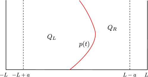
Following [1], we define evolving Bochner spaces on these domains. We present the construction for the left domain only, since the argument for the right domain is analogous. First denote by the evolving Hilbert space. Next we define the map by
with and for all and . The function is obviously continuous and reduces to the identity at . It is also a homeomorphism as its inverse
is continuous as well. This allows us to introduce the evolving Bochner spaces (as in [1, Definition 2.7])
| (2.7) | ||||
| (2.8) |
and, following again [1], make the identification of with for (and likewise in ). The space of continuously differentiable functions on evolving Bochner spaces is given by
Thus we can, as in [1, Definition 2.20], to give a notion of time (material) derivative as
for any . Then we can finally define the space used for the notion of weak solutions, namely
| (2.9) |
The definitions of the respective quantities , , , and
are analogous.
While the previous definitions allow us to directly work in a noncylindrical domain, it is sometimes also useful consider the transformation to the fixed domain . Hence we introduce transformations which map and to :
| (2.10a) | ||||||
| (2.10b) | ||||||
Note that due to assumption (A1), and are well-defined and that actually flips the domain, i.e. it swaps left and right boundary points.
2.4 Adjoint equations
The next ingredient will be two adjoint equations, posed on the domains and , respectively.
Definition 2.5 (Adjoint equations).
For any , , , and , we introduce the backward in time adjoint equations
| (2.11a) | ||||||
| (2.11b) | ||||||
| (2.11c) | ||||||
| (2.11d) | ||||||
and
| (2.12a) | ||||||
| (2.12b) | ||||||
| (2.12c) | ||||||
| (2.12d) | ||||||
Applying the existence theory of, e.g. [1], for equations on evolving domains, we obtain the following theorem.
Theorem 2.6.
With the help of the transformations and , equation (2.11) and (2.12) can be transformed into a generic problem of the form
| (2.15a) | ||||||
| (2.15b) | ||||||
| (2.15c) | ||||||
| (2.15d) | ||||||
For (2.11) we define and compute
| (2.16) |
while for (2.12) and we obtain
| (2.17) |
Note that in view of Lemma 2.3 and Assumption (A1), the coefficients and are (in both cases) continuous and uniformly bounded by
| (2.18) |
as there may be points with . Thus, standard existence and regularity results for linear diffusion–convection equations on fixed domains, such as [15, Theorem 5.2], can be used to ensure the solvability of (2.15).
3 Data assimilation problem
We now turn to the main part of this paper - the inverse or data assimilation problem 1. In classic data assimilation approaches one would use the measurements of and on to reconstruct the initial datum of (1.1). Here we follow an alternative approach proposed by Puel et al., see [20, 21], and estimate the buyer-vendor distribution at the final time, that is instead. This requires the solution of additional optimal control problems, which are, however, well posed if an appropriate regularisation (penalty) is added.
To use Puel’s strategy in our setting, we will estimate the densities of buyers and of vendors separately (that is on the right and left of the free boundary). The reconstruction is based on the following two duality estimates:
Theorem 3.1.
Proof.
Now we will use (3.2a)–(3.2b) to determine . Since the choice of and in (3.2a) and (3.2b) is arbitrary and the last term on the right hand side contains only known (i.e. computed or measured) quantities, we could obtain a linear functional of . The only unknowns are the first terms on the respective right hand sides. But since we are free to choose arbitrary boundary data and , this leads to the null–controllability problems for (2.11)–(2.12). Indeed, if we can chose and such that and , the unknown terms in both orthogonality relations drop out and we can reconstruct .
3.1 Optimal control problem
To conduct the strategy outlined above, we have to solve the optimal control problems
| (3.3) | ||||
| (3.4) |
Since the structure of both problems is the same, we will only discuss the first one. To increase readability, we will drop the subscript and write , , instead of , from now on. The next result states that the optimal control problem is indeed exactly null-controllable in the sense of the following definition.
Definition 3.2.
The following exact boundary controllability result is based on [7, Theorem 2.3], slightly extended and adapted to our situation. The theorem reads as follows.
Theorem 3.3 (Exact null-controllability).
For every , there exists at least one control such that the solutions of (2.11) satisfies on . Furthermore, there exists a constant which depends on , and such that
| (3.5) |
holds with being the control of minimum –Norm.
Proof.
The regularity of the price allows us to transform the problem to a fixed domain using defined in (2.10). Hence we only consider equations of type (2.15). First we observe that for any positive , any solution to (2.15) with initial datum is, by standard parabolic regularity [12, Chapter 7.1], in with the estimate
| (3.6) |
Thus, we can assume that already holds. Since by lemma 2.3, (and thus the coefficients and in (2.15) are continuous) we can apply [7, Theorem 2.3] to conclude the requested boundary controllability. The continuity estimate (3.5) then follows by combining (3.6), the respective estimate from [7, Theorem 2.1] for the distributed control problem and a standard trace inequality.
∎
In order to be able to numerically solve the optimal control problem, we introduce the following regularized version
| (3.7) |
Standard arguments guarantee the existence of a unique minimizer, see e.g. [22, Section 3.5]. Calculating the derivatives of the corresponding Lagrange functional
| (3.8) | ||||
we obtain the first order optimality system
| (3.9a) | |||||
| (3.9b) | |||||
| (3.9c) | |||||
| (3.9d) | |||||
where satisfies the adjoint equation (2.11) and the coupling
| (3.10) |
The following results examine the convergence of as . The proofs are using the same techniques as in [21], yet adapted to our boundary control problem.
Theorem 3.4.
Proof.
By Theorem 3.3, we know that there exists at least one function solving the exact null controllability problem. Thus, the set of all these controls in is nonempty. As it is also convex and closed, there exists a unique having minimal -norm. Since minimizes the functional (3.7) among all function in we have
| (3.13) |
which implies the (uniform in ) bound
| (3.14) |
Thus, we can extract a subsequence, again labelled that converges weakly to some in . Using the weak formulation of (2.11) and an Aubin-Lions argument, we see that this is sufficient to obtain the convergence
and (3.13) implies Thus, arguing as in the proof of [21, Theorem 2.12], we can use the fact that has minimal norm as well as the lower semi-continuity of the norm w.r.t weak convergence to obtain that . This argument also implies norm convergence and the uniqueness of the limit then finally yields
This also implies which completes the proof. ∎
Remark 3.5.
Understanding the optimal control problem (3.3) (or (3.4)) as Tikhonov regularisation, one could ask for convergence rates of to as . Indeed, such rates could be expected under appropriate source conditions on . The interesting point now is to understand the influence of in the definition of the forward operator in the characterisation of such conditions and also how perturbation in would influence them. We leave this question for future research.
4 Stability in the presence of measurement errors
Assume we have measurements of two different prices and as well as two different transaction rates and . Can we control the difference in the reconstructions and as well as the future predicted prices and for in terms of these differences? In this section we will give a positive answer to this question based on the following strategy
-
1.
Estimate the error in the optimal controls and in terms of the error in and (Lemma 4.2).
-
2.
Estimate the error in the respective reconstructions and in terms of errors in price and transaction rate (Lemma 4.3).
-
3.
Use these results to predict errors in the future price (Lemma 4.7).
Note however that for the last point we need to make additional regularity assumptions on the reconstructed final data that do not directly follow from our analysis (see Remark 4.5 for details). We start by assuming
-
(A3)
W.l.o.g. we only consider the optimality system related to (3.3), i.e. the left part and again drop the subscript . Moreover, we transform all equations to the unit interval , so that the optimality system reads as
| (4.1a) | |||||
| (4.1b) | |||||
| (4.1c) | |||||
| (4.1d) | |||||
| (4.1e) | |||||
| (4.1f) | |||||
| (4.1g) | |||||
| (4.1h) | |||||
| and the coupling condition | |||||
| (4.1i) | |||||
with and as defined in (2.16). Note that the transformed primal and dual equations are still adjoint to one another, yet now with respect to the scalar product
| (4.2) |
Proof.
Now we are able to prove stability of the optimal control problem in terms of measurement errors in the price.
Lemma 4.2 (Stability of ).
Proof.
For each (and corresponding , ), we denote by , and the corresponding solutions to the optimality system (4.1a)–(4.1i) and furthermore
Then, and satisfy, in the weak sense, the equations
| (4.3a) | ||||||
| (4.3b) | ||||||
| (4.3c) | ||||||
| (4.3d) | ||||||
| and | ||||||
| (4.3e) | ||||||
| (4.3f) | ||||||
| (4.3g) | ||||||
| (4.3h) | ||||||
Note that the following calculations are formal since for now we only know existence of weak solutions and therefore some of the integrals are not defined. In the end we arrive, however, at an estimate which is again well defined and could can be obtained rigorously by directly working with weak solutions. We chose this way of presentation as we believe it to be easier to follow. Thus (formally) taking equation (4.3a) and testing it with (with respect to the scalar product (4.2)) yields
Integrating by parts on the left hand side, using (4.3e) and the boundary conditions results in
A final integration by parts to remove the second derivatives on the right hand side gives
Using the estimates of Lemma 4.1, the boundedness of in (see (3.14)) and Cauchy’s inequality applied to the last term on the right hand side, we have
where we also used the lower bounds (2.18) on and Assumption (A3) to estimate the expression from below by and above by . Using again (2.18) yields
Combining this with the previous estimate yields the assertion. ∎
For the second step of our strategy, we return to the orthogonality relation (3.2a) which, transformed to , reads as
| (4.4) | ||||
In the presence of errors in and we obtain two different relations and the following stability result. Note that the above results on the adjoint equations imply solvability for with continuous dependence on the initial value for any . Hence, the duality relation uniquely defines when given . There is further stable dependence of on the errors in the price and transaction rates, which we make precise by the following result:
Lemma 4.3 (Stability of ).
Proof.
Subtracting (4.4) for and yields
We estimate each term of the right hand side separately
where we used Lemmata 4.1 and 4.2. Next we have
using that for positive times (and away from the boundary) is Lipschitz continuous. Next we have
and finally
Combining all estimates and taking the supremum over all with , we finally obtain
| (4.5) |
Taking yields the assertion. ∎
Remark 4.4.
The estimates of Lemma 4.2 and 4.3 show that, for , the reconstruction of the unknown buyer vendor distribution is actually a well-posed problem, at least for sufficiently smooth perturbations of . This is due to the fact that we are solving a regularized optimization problem. The price to pay is that the term involving in (4.4) does not vanish. However, since is fixed, is does not appear in our stability estimates.
For the next result, we choose perturbed prices and such that and assume w.l.o.g. that and make the following additional assumptions:
-
(A4)
,
-
(A5)
with
-
(A6)
Remark 4.5.
We mention that indeed it is natural to assume strong regularity of in a neighbourhood of for , since it locally arises as the solution of a heat equation. On the other hand we need to expect some singularities around and due to the singular source terms. Thus (A5) seems completely natural for forwards solutions of the price formation model. Moreover, it can also be verified that reconstructed via (4.4) has local -regularity, which follows from using supported in and an analysis of the solution of the parabolic equation for , which can be estimated in terms of the norm of the initial value.
In the following we analyse the forward propagation for in a small time interval. We denote the new initial value by . First note that using the same localisation strategy as in [19] (i.e. multiplying the solution to (1.1) with a smooth cut-off function that has support inside the interval ), implies
| (4.6) |
with to be fixed later on and where is the solution to (1.1) with the reconstructed initial datum that additionally satisfies (A4)-(A6). Furthermore, is an interval that is compactly contained in . This allows us to derive the following estimates on terms of the form , where we denote by the heat kernel with Neumann boundary conditions on , see e.g. [6, Section 6.4], and furthermore use the notation
Lemma 4.6.
Proof.
First note that is the solution to the heat equation with homogeneous Neumann boundary condition, zero right hand side and initial datum . Then, the first estimate is a direct consequence of (4.6) applied to such an solution with initial datum . The second one follows from the fact that, as for sufficiently small, and are in and thus, using again (4.6), the derivative of a solution to the heat equation that appears on the left hand side is Lipschitz continuous. ∎
We are now in a position to state the stability result for future prices.
Lemma 4.7.
Note that unfortunately, we cannot give a lower bound on the quantity as it depends in a non-linear and non-local fashion on the initial datum via the solution of the equation. However, the proof below shows that as the transaction rate increases, also becomes larger which agrees with the modelling.
Proof.
Due to assumption (A5) we can invoke [19][Lemma 2.5] to show that for sufficiently small (depending on , ) the corresponding transaction rates are strictly positive on . Furthermore, (A5) implies that are in . Now Duhamel’s formula allows us to express the solutions to (1.1) as
| (4.7) |
Taking the space derivative and evaluating at we obtain
| (4.8) |
Subtracting (4.8) for and using the linearity of the convolution, we obtain
| (4.9) | ||||
with As the are continuous, choosing sufficiently small guarantees that the derivatives of appearing in the definition of are always evaluated away from their singularity, in particular they are bounded and locally Lipschitz-continuous, which implies with the local Lipschitz constant
Taking the absolute value on both sides of (4.9) and using Lemma 4.6 implies
so that Gronwall’s lemma implies, together with (A3) and (A6), yields
| (4.10) |
Next we exploit the fact that by taking the time derivative, which gives
Subtracting the above equation for and respectively, using the definition of and integrating in time we obtain, for
| (4.11) | ||||
Denoting by and using (A3) this yields
As a consequence of (4.6), is bounded and Lipschitz continuous. Thus using (4.10), (A3) and once more (4.6) applied to (and together with (A6)) finally yields the assertion. ∎
5 Numerical Simulation
We conclude by illustrating the proposed methodologies and confirming the
obtained analytic results with various computational experiments. All simulations are
performed on
the domain , which is split into intervals of length . The
discrete grid points are denoted by . We compute solutions at
discrete times , where is the discrete time
step. However we will omit all full time-discrete expressions in the
following, to enhance readability.
The reconstruction of the
buyer-vendor distribution is based on piecewise linear basis functions.
Let denote the space of piecewise linear basis functions , which
satisfy . We wish to reconstruct , which is given by
using the duality estimates (3.2).
Data generation: We solve the transformed LL model (2.2)
for a given initial buyer-vendor distribution . In doing so we transform the
initial distribution via (2.1), and compute the solution to the heat
equation (2.2) using an implicit in time discretization. The
returned discrete price corresponds to the
zero levelset of the buyer-vendor distribution (computed via linear
interpolation). Note that we use a
finer spatial and temporal discretization to generate the data than in the subsequent
reconstruction.
Steepest descent: We solve (3.7) and the corresponding problem on and using steepest descent. In doing so, we compute the variational derivatives of (3.8) and obtain the first order optimality system (3.9) as well as the updates for the controls and . The detailed steps are outlined in the While-Loop of Algorithm 5.1. Here the parameter is the step size of the steepest descent update. We use the Armijo-Goldstein condition to adjust in the search direction . We recall that the Armijo-Goldstein condition for a general functional is given by
| (5.1) |
where . The starting value is set to , which is then reduced (up to a maximum of four times) by a factor of until condition (5.1) is satisfied. Note that we transform the computational domains and to as discussed in Section 2.3 in all simulations. We solve the forward as well as the adjoint equations using an implicit in time discretization and piecewise linear basis functions in space.
Identifiabilty for different initial conditions.
In the first experiment we set and the final time to . We split the spatial domain into elements and the time interval into time steps. The initial datum is set to
| (5.2) |
We approximate the final buyer-vendor distribution using basis functions. Furthermore we choose the following parameters
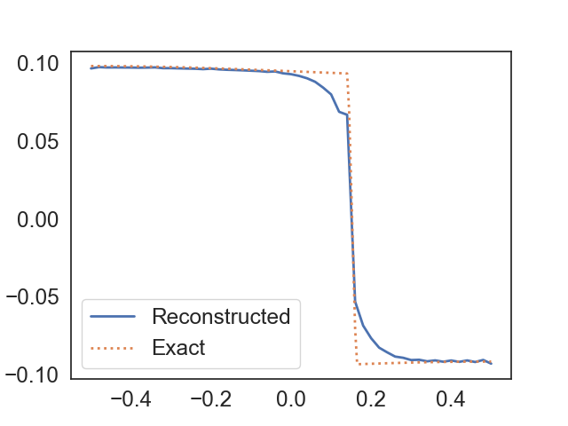
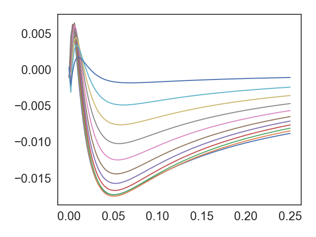
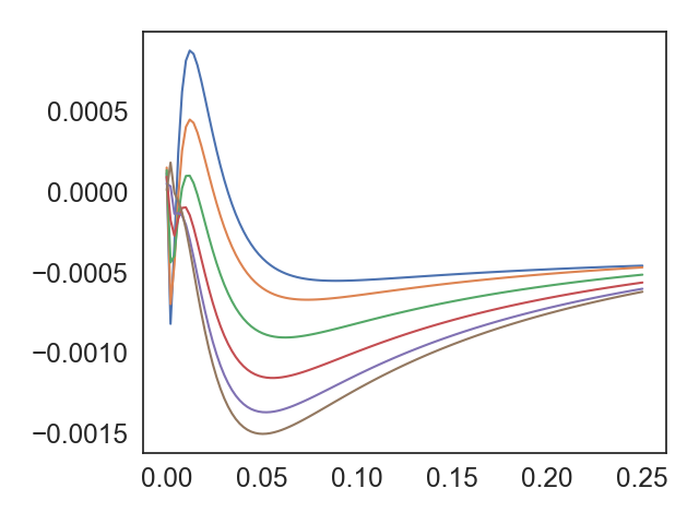
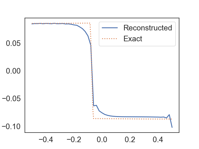
Figure 2 shows the reconstructed and computed function (the latter computed by solving the heat equation (2.2) with the transformed initial datum ). We observe a good agreement, with small artefacts at the boundary and the buyer-vendor interface. The corresponding controls are shown in Figure 3.
Next we choose a slightly different initial datum, in particular
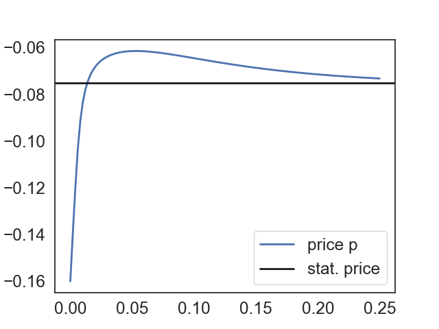
In this case the price is not monotone, see Figure 4. However, the quality of the reconstructions is comparable to the one of the previous example.
Stability of
Next we are interested in the stability of the reconstruction with respect to perturbations in the price. Lemma 4.3 and in particular estimate (4.5) state that the difference in the reconstructions is bounded by the difference in the prices and transaction rates. We consider the following perturbation of the unperturbed price :
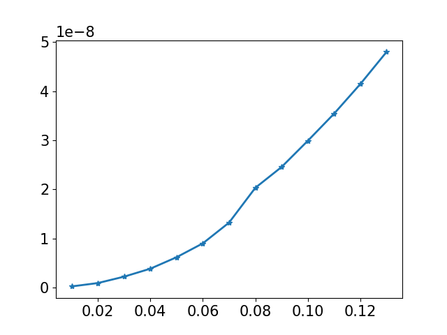
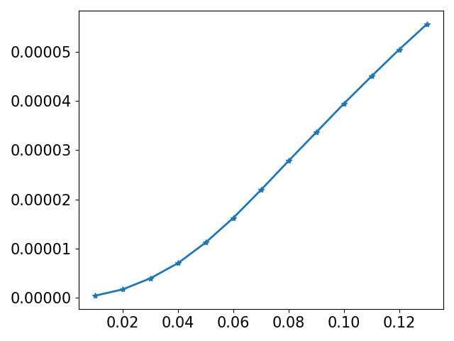
Note that the perturbed price is still in and that for all . We start with the same the initial datum as in the first example, that is (5.2), and set and . All other parameters are the same as in the first example, except that we reconstruct the final profile using basis functions. Figure 5 illustrates the linear increase of the error in the controls and the reconstruction as the noise level increases. For larger values of this agrees with the theoretical results of Lemma 4.2 and Lemma 4.3, respectively. For small a saturation effect due to the numerical discretization error occurs.
Predicting price dynamics
We conclude with an example where we use the reconstructed buyer-vendor distribution to estimate future price dynamics and illustrate the influence of noise in those. We consider an initial datum of the form
on the domain , that is . The computational domain is split into intervals, the time horizon into time steps. Since the number
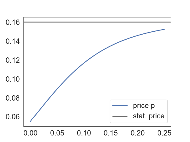
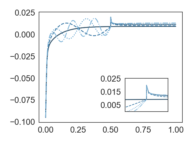
of buyers equals the number of vendors the exact price is constant and equal to zero. The computed price curve, that is the dark blue line in Figure 6, converges
quickly to the true equilibrium price (being slightly off at the beginning due to numerical errors caused by the nonlinear transformation of the initial datum).
We then use the original price curve on the time interval , denoted by , as well as the perturbed prices
to reconstruct the solution at time , that is . Note that the sinusoidal perturbations ensure that the final distribution of buyers and vendors equals the initial
distribution. These reconstructed buyer-vendor profiles are then used to compute the future price dynamics. We observe a jump in the price in all prices at time , which
is caused by the numerical error made in the reconstruction. However, the price then converges quickly to an equilibrium value, which is close to the true price (dark blue line).
The parameters used in the reconstruction Algorithm 5.1 are set to
The final buyer vendor distribution was computed using basis functions.
6 Summary and Outlook
We studied a data assimilation problem for a parabolic nonlinear free boundary problem. This partial differential equation describes the
evolution of the price, that is the free boundary, in a large economic market. We developed an analytical and computational framework for
the corresponding data assimilation problem, which is based on a previous work by Puel et al., see [20]. The free boundary splits the original problem into two
parts, each of them defining a separate optimal control problem. We discussed analytic properties of the respective problems and derived
stability estimates for the controls and reconstructed unknown buyer-vendor distribution in the presence of noise. Finally we confirmed and illustrated our
results with computational experiments.
We believe that the developed framework provides the basis for more general data assimilation problems in price formation. In [2] Burger et al. considered a Boltzmann type price formation
model, which allows for more complex trading mechanisms. This problem is a system of nonlocal reaction-diffusion equations on the whole domain, where multiple prices (even with continuous distribution) and transaction rates can appear. Analogous questions can be asked for this problem if only the expectation of the price is to be predicted, but the problem could also be extended to a stochastic distribution of the price.
Acknowledgements
MB acknowledges support by ERC via Grant EU FP 7 - ERC Consolidator Grant 615216 LifeInverse. MTW acknowledges financial support from the Austrian Academy of Sciences ÖAW via the New Frontiers Grant NST-001 and the EPSRC via the First Grant EP/P01240X/1.
References
- [1] A. Alphonse, C. M. Elliott, and B. Stinner. An abstract framework for parabolic PDEs on evolving spaces. Portugaliae Mathematica, 72:1–46, 2015.
- [2] M. Burger, L.A. Caffarelli, P.A. Markowich, and M.-T. Wolfram. On a Boltzmann-type price formation model. 469(2157):20130126, 2013.
- [3] M. Burger, L.A. Caffarelli, P.A. Markowich, and M.-T. Wolfram. On the asymptotic behavior of a Boltzmann-type price formation model. Communications in Mathematical Sciences, 12(7), 2014.
- [4] L.A. Caffarelli, P.A. Markowich, and J.-F. Pietschmann. On a price formation free boundary model by Lasry and Lions. Comptes Rendus Mathematique, 349(11-12):621 – 624, 2011.
- [5] L.A. Caffarelli, P.A. Markowich, and M.-T. Wolfram. On a price formation free boundary model by Lasry and Lions: the Neumann problem. Comptes Rendus Mathematique, 349(15):841–844, 2011.
- [6] J.R. Cannon. The one-dimensional heat equation, volume 23 of Encyclopedia of Mathematics and its Applications. Addison-Wesley Publishing Company, Advanced Book Program, Reading, MA, 1984. With a foreword by Felix E. Browder.
- [7] D. Chae, O.Y.. Imanuvilov, and S.M. Kim. Exact controllability for semilinear parabolic equations with Neumann boundary conditions. Journal of Dynamical and Control Systems, 2(4):449–483, 1996.
- [8] L. Chayes, M. del Mar González, M.P. Gualdani, and I. Kim. Global existence and uniqueness of solutions to a model of price formation. SIAM Journal on Mathematical Analysis, 41(5):2107–2135, 2009.
- [9] C. Clason and P. Hepperger. A forward approach to numerical data assimilation. SIAM Journal on Scientific Computing, 31(4):3090–3115, 2009.
- [10] R. Cont and M. S. Mueller. A stochastic PDE model for limit order book dynamics. arXiv e-prints, page arXiv:1904.03058, Apr 2019.
- [11] M. del Mar Gonzàlez and M. P. Gualdani. Asymptotics for a free boundary model in price formation. Nonlinear Analysis: Theory, Methods & Applications, 74(10):3269 – 3294, 2011.
- [12] L. C. Evans. Partial differential equations, volume 19 of Graduate Studies in Mathematics. American Mathematical Society, Providence, RI, second edition, 2010.
- [13] M. Hinze, R. Pinnau, M. Ulbrich, and S. Ulbrich. Optimization with PDE constraints, volume 23. Springer Science & Business Media, 2008.
- [14] M. V. Klibanov. Inverse problems and Carleman estimates. Inverse problems, 8(4):575, 1992.
- [15] O. A. Ladyzenskaja, V. A. Solonnikov, and N. N. Ural’ceva. Linear and Quasilinear Equations of Parabolic Type. American Mathematical Society, Providence, rhode island, 1968.
- [16] J.-M. Lasry and P.-L. Lions. Mean field games. Jpn. J. Math., 2(1):229–260, 2007.
- [17] J. L. Lions. Control and estimation in distributed parameter systems: 1. Pointwise control for distributed systems. chapter 1, pages 1–39. SIAM, 1992.
- [18] P. Markowich, J. Teichmann, and M. Wolfram. Parabolic free boundary price formation models under market size fluctuations. Multiscale Modeling & Simulation, 14(4):1211–1237, 2016.
- [19] P.A. Markowich, N. Matevosyan, J.-F. Pietschmann, and M.-T. Wolfram. On a parabolic free boundary equation modeling price formation. Mathematical Models and Methods in Applied Sciences, 19(10):1929–1957, 2009.
- [20] J.-P. Puel. Une approche non classique d’un problème d’assimilation de données. Comptes Rendus Mathematique, 335(2):161 – 166, 2002.
- [21] J.-P. Puel. A Nonstandard Approach to a Data Assimilation Problem and Tychonov Regularization Revisited. SIAM Journal on Control and Optimization, 48(2):1089–1111, 2009.
- [22] F. Tröltzsch. Optimal control of partial differential equations: theory, methods, and applications, volume 112. American Mathematical Soc., 2010.
- [23] M. Yamamoto. Carleman estimates for parabolic equations and applications. Inverse problems, 25(12):123013, 2009.