PowerSGD: Practical Low-Rank
Gradient Compression for Distributed Optimization

Abstract

We study lossy gradient compression methods to alleviate the communication bottleneck in data-parallel distributed optimization. Despite the significant attention received, current compression schemes either do not scale well, or fail to achieve the target test accuracy. We propose a new low-rank gradient compressor based on power iteration that can i) compress gradients rapidly, ii) efficiently aggregate the compressed gradients using all-reduce, and iii) achieve test performance on par with SGD. The proposed algorithm is the only method evaluated that achieves consistent wall-clock speedups when benchmarked against regular SGD using highly optimized off-the-shelf tools for distributed communication. We demonstrate reduced training times for convolutional networks as well as LSTMs on common datasets. Our code is available at https://github.com/epfml/powersgd.

1 Introduction

Synchronous data-parallel SGD is the most common method for accelerating training of deep learning models (Dean et al., 2012; Iandola et al., 2015; Goyal et al., 2017). Because the gradient vectors of such models can be large, the time required to share those gradients across workers limits the scalability of deep learning training (Seide et al., 2014; Iandola et al., 2015; Lin et al., 2018).

Previous work proposes lossy gradient compression as a solution to this issue. Notable examples include replacing the coordinates of the gradient with only their sign (Seide et al., 2014; Carlson et al., 2015; Bernstein et al., 2018, 2019; Karimireddy et al., 2019), quantizing the individual coordinates (Alistarh et al., 2017; Wen et al., 2017), and low-rank approximation of the gradient (Wang et al., 2018). While these works demonstrate speedups over full-precision SGD in some settings, we find that their speedups vanish with a fast network and highly optimized communication backend, even on commodity hardware. Some prior work also suffers from degraded test accuracy compared to SGD. We combine three observations to fix these issues: i) Linear compressor operators achieve scalability by enabling aggregation using all-reduce. ii) Error feedback ensures convergence with general biased compressors. iii) Low-rank updates enable aggressive compression without sacrificing quality.

First, we explore the properties of various gradient compression schemes for SGD and identify which ones are crucial for high scalability. In particular, we note that currently proposed gradient compressors are not linear. Their compressed messages cannot be added up hierarchically, unlike raw gradients. This prevents current compressed SGD algorithms from aggregating gradients using an efficient reduce operation and instead require a gather operation. Current deep learning frameworks rely either solely or predominantly on all-reduce, which is key to why regular SGD scales well with fast communication hardware (cf. Awan et al., 2018; Panda et al., 2019).

Secondly, it was recently shown that using error feedback (i.e. storing the difference between the computed and compressed gradient, and reinserting it at the next iteration) improves both convergence and generalization for compression schemes (Karimireddy et al., 2019). This can enable general biased gradient compression schemes to reach the target test accuracy.

Thirdly, there is growing evidence that the generalization ability of modern over-parameterized deep learning models is related to low-rankedness (Arora et al., 2018; Martin & Mahoney, 2018; Collins et al., 2018). Using a low-rank update (as we do) can be viewed as implicitly performing spectral regularization (Gunasekar et al., 2018) and hence can be expected to have good generalization properties (Yoshida & Miyato, 2017). Further, Wang et al. (2018) show that the eigenspectrum of the stochastic gradients for deep learning models decays, suggesting that a rank-based schemes can get away with aggressive compression without sacrificing convergence.

In this work, we design PowerSGD with the above observations in mind. PowerSGD computes a low-rank approximation of the gradient using a generalized power iteration (known as subspace iteration (Stewart & Miller, 1975)). The approximation is computationally light-weight, avoiding any prohibitively expensive Singular Value Decomposition. To improve the quality of the efficient approximation, we warm-start the power iteration by reusing the approximation from the previous optimization step. Using all-reduce gradient aggregation, we empirically demonstrate that PowerSGD achieves wall-clock speedups over regular SGD in a 16-GPU setting, even with the optimized NCCL communication backend on a fast network (and is the only algorithm to do so.) By compressing gradients more than $120\times$, we reduce communication time (including coding and decoding) by $54\%$ for ResNet18 on Cifar10 and by $90\%$ for an LSTM on Wikitext-2. End-to-end wall-clock training time to full test quality is reduced by $24\%$ for ResNet18 and by $55\%$ for the LSTM.

2 Related work

Layer gradient

Sign

Sign $+$ Norm

Top $K$

Random $K$

Random Block

Low-rank (ours)

Figure 1: Compression schemes compared in this paper. Left: Interpretation of a layer’s gradient as a matrix. Coordinate values are color coded ( positive, negative). Right: The output of various compression schemeson the same input. Implementation details arein Appendix G.

Gradient compression

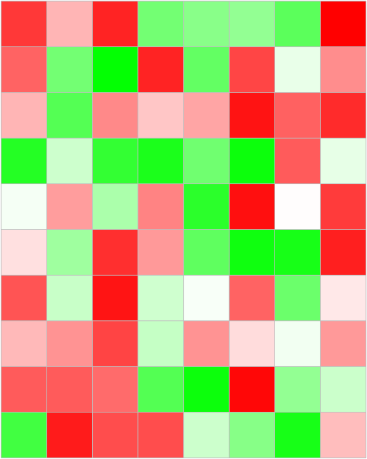
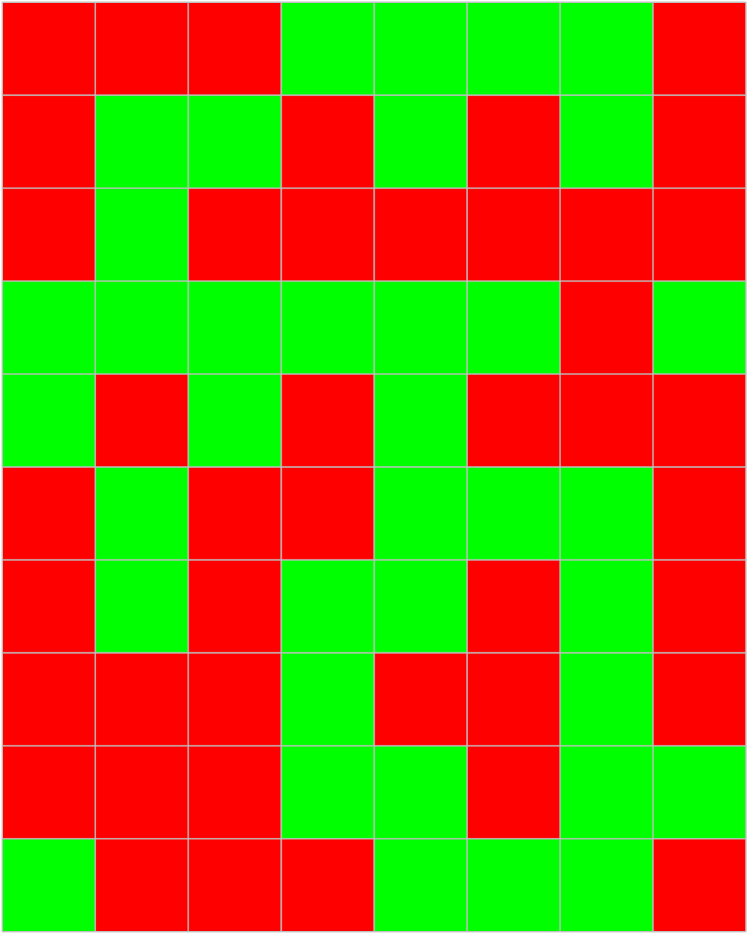
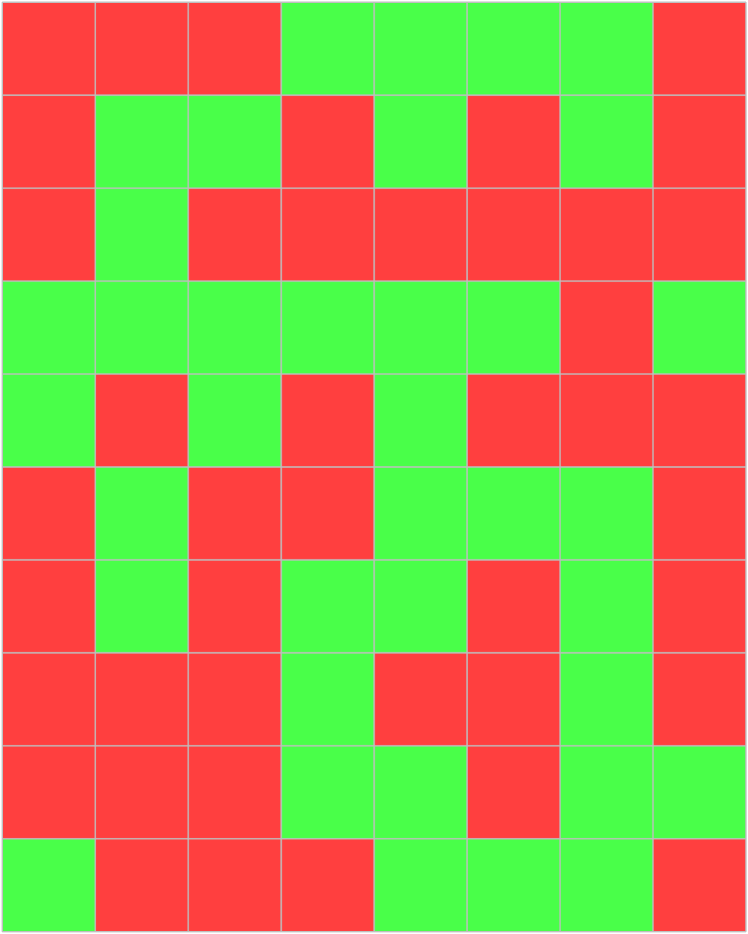
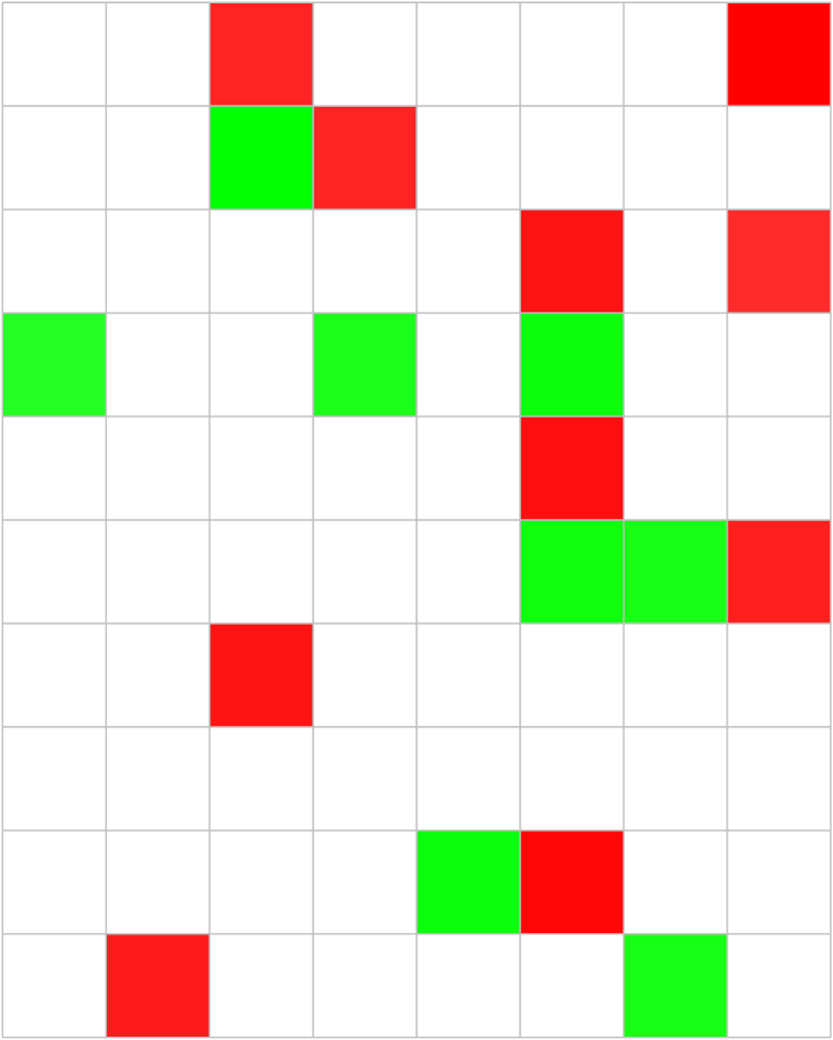
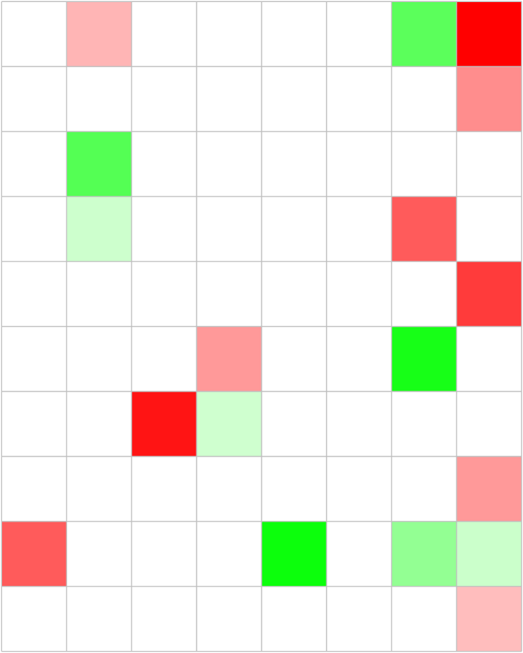
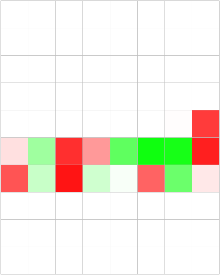
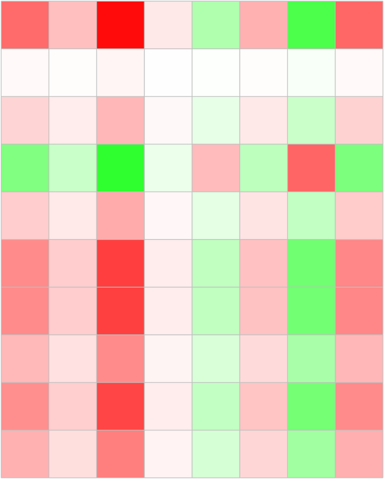
A variety of compression schemes (Figure 1) have been proposed: Alistarh et al. (2017) and Wen et al. (2017) quantize each gradient coordinate; Seide et al. (2014); Carlson et al. (2015); Bernstein et al. (2018, 2019) and Karimireddy et al. (2019) replace each coordinate of the gradient with its sign; Lin et al. (2018); Stich et al. (2018) and Wangni et al. (2018) use the largest few coordinates; and Konečnỳ et al. (2016) and Wang et al. (2018) use a low-rank approximation.

Spectral Atomo by Wang et al. (2018) is perhaps the closest to our work. It performs importance sampling of the gradient’s singular vectors and is an unbiased compression scheme. It requires, however, a full Singular Value Decomposition every iteration and is hence computationally impractical.

Commutative compression and addition

Yu et al. (2018) stress that commutability of compression with gradient addition enables efficient aggregation with ring all-reduce. Most compressors, however, lack this property. Yu et al. utilize temporally-consistent correlations between gradients coordinates to compress them linearly. PowerSGD has a similar property that we call ‘linearity’.

Error feedback

First introduced in (Seide et al., 2014) and analyzed in (Stich et al., 2018) for the convex case, error feedback involves computing the difference between a worker’s gradient and the compressed gradient (i.e. error) and adding it back to the next gradient (feedback). Karimireddy et al. (2019) and Stich & Karimireddy (2019) further develop and generalize the framework of error feedback with improved rates. In the non-convex setting, Karimireddy et al. (2019) show that error feedback is crucial both for convergence and generalization when using biased compressors (e.g. sign or top-$K$). In general, biased compression schemes equipped with error feedback tend to out-perform their unbiased counterparts. The practical algorithm by Lin et al. (2018) is also as an approximate top-$K$ compressor with error feedback.

Low-rank methods

Recent works argue that in modern over-parameterized deep networks, the final model learnt has a ‘low stable rank’ (Martin & Mahoney, 2018; Li et al., 2018). This can partially explain their impressive generalization properties despite being substantially overparameterized (Arora et al., 2018). Adding explicit spectral regularization has shown to further improve the performance of such models (Mazumder et al., 2010; Yoshida & Miyato, 2017). Using a low-rank update (as we do) can be viewed as implicitly performing a similar regularization (Gunasekar et al., 2018). If the target matrices are known to be exactly low-ranked (instead of just low stable rank), Yurtsever et al. (2017) show that it is sometimes possible to converge to the optima using low rank approximations of the gradients without the need for error feedback.

3 Method

In data-parallel optimization of machine learning models, a number of $W$ workers share the same model parameters $\mathbf{x}\in\mathbb{R}^{d}$. They iteratively update $\mathbf{x}$ by computing independent stochastic gradients, aggregating these gradients by averaging, and updating the model parameters based on this aggregate.

Algorithm 1 Rank-$r$ PowerSGD compression

1:The update vector $\Delta_{w}$ is treated as a list of tensors corresponding to individual model parameters. Vector-shaped parameters (biases) are aggregated uncompressed. Other parameters are reshaped into matrices. The functions below operate on such matrices independently. For each matrix $M\in\mathbb{R}^{n\times m}$, a corresponding $Q\in\mathbb{R}^{m\times r}$ is initialized from an i.i.d. standard normal distribution.

2:function compress+aggregate(update matrix $M\in\mathbb{R}^{n\times m}$, previous $Q\in\mathbb{R}^{m\times r}$)

3:     $P\leftarrow MQ$

4:     $P\leftarrow\textsc{all reduce mean}(P)$ $\triangleright$ Now, $P=\frac{1}{W}(M_{1}+\ldots+M_{W})Q$

5:     $\hat{P}\leftarrow\textsc{orthogonalize}(P)$ $\triangleright$ Orthonormal columns

6:     $Q\leftarrow M^{\top}\hat{P}$

7:     $Q\leftarrow\textsc{all reduce mean}(Q)$ $\triangleright$ Now, $Q=\frac{1}{W}(M_{1}+\ldots+M_{W})^{\top}\hat{P}$

8:     return the compressed representation $(\hat{P},Q)$.

9:end function

10:function decompress($\hat{P}\in\mathbb{R}^{n\times r}$, $Q\in\mathbb{R}^{m\times r}$)

11:     return $\hat{P}Q^{\top}$

12:end function

PowerSGD compression

We approximate each layer in the model independently. The parameters of fully-connected layers (dense matrix multiplication) and their gradients have an inherent matrix structure. The parameters of convolutional layers can be naturally interpreted as fully-connected layers applied repeatedly over a 2D grid of inputs. Practically, this amounts to flattening input and kernel dimensions in the 4D gradient tensors. Neural networks also contain bias vectors, but these typically constitute a tiny fraction of the parameter space and can be aggregated uncompressed.

For each parameter’s gradient $M\in\mathbb{R}^{n\times m}$, the aim of rank-$r$ matrix approximation is to find matrices $P\in\mathbb{R}^{n\times r}$ and $Q\in\mathbb{R}^{m\times r}$ such that $PQ^{\top}$ approximates $M$ well. PowerSGD uses a single step of subspace iteration—power iteration generalized to $r>1$—to compute such an approximation. This involves performing one right multiplication, one left multiplication, and an orthogonalization. We use the Gram-Schmidt procedure to orthogonalize our matrices since they have very few columns (1–4), and this is the most expensive part of the compression procedure. Further, we ‘warm-start’ the subspace iteration by reusing the approximation computed at the previous step. With the inclusion of warm-start, a single step of subspace iteration yields a factorization $M\sim PQ^{\top}$ with the same performance as the best rank-$r$ approximation from an expensive Singular Value Decomposition.

Efficient aggregation between workers

In data-parallel optimization, we want to approximate the average of the worker’s gradients. Suppose PowerSGD operates on a list of corresponding gradients $\left[M_{1}\ldots M_{W}\right]$ from $W$ workers. Both occurrences of $M$ in the algorithm are a (linear) matrix multiplication followed by a (linear) mean reduction over workers. This introduces a practical invariance: execution on 1 worker with batch size $B\times W$ is equivalent to execution on $W$ workers with batch size $B$ each. We call this property ‘linearity’. Refer to Appendix A.3 for more details.

(a) Gather

(b) Reduce

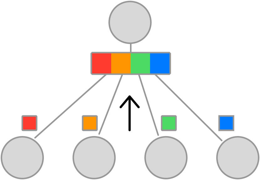
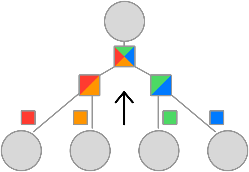
An important benefit of the PowerSGD’s linearity is that it can be implemented using the all-reduce protocol as opposed to needing a gather operation. To illustrate the difference, suppose that we want to compute the sum of $W$ matrices $\sum_{i=1}^{W}M_{i}$ for $W=4$. The all-reduce method can use associativity of addition to rewrite the computation as $(M_{1}+M_{2})+(M_{3}+M_{4})$. This enables a divide-and-conquer approach and allows the summation task to be split over multiple workers, as illustrated on the right. With $W$ workers, both the computation and the communication time scale as $\mathcal{O}(\log W)$ for all-reduce, compared to $\mathcal{O}(W)$ for all-gather.

In addition to improved scaling, all-reduce communication is preferred over a parameter-server setting because it avoids double compression. With a parameter server, both the ‘clients $\rightarrow$ server’ and ‘server $\rightarrow$ clients’ communication have to be compressed (Caldas et al., 2018; Bernstein et al., 2019; Seide et al., 2014). We avoid this by merging compression and aggregation into one step.

Error-feedback SGD

Since the PowerSGD scheme is biased (i.e. compressing and decompressing a random gradient does not yield the original in expectation), we use error feedback (Seide et al., 2014; Karimireddy et al., 2019). Our version of error feedback (Algorithm 2) extends the original by introducing post-compression momentum. This simple extension allows us to reuse the same learning rate and hyper-parameters as those tuned for SGD with momentum.

Algorithm 2 Distributed Error-feedback SGD with Momentum

1:hyperparameters: learning rate $\gamma$, momentum parameter $\lambda$

2:initialize model parameters $\mathbf{x}\in\mathbb{R}^{d}$, momentum $\mathbf{m}\leftarrow\mathbf{0}\in\mathbb{R}^{d}$, replicated across workers

3:at each worker $w=1,\ldots,W$ do

4:     initialize memory $\mathbf{e}_{w}\leftarrow\mathbf{0}\in\mathbb{R}^{d}$

5:     for each iterate $t=0,\ldots$ do

6:         Compute a stochastic gradient $\mathbf{g}_{w}\in\mathbb{R}^{d}$.

7:         $\Delta_{w}$ $\leftarrow\mathbf{g}_{w}+\mathbf{e}_{w}$ $\triangleright$ Incorporate error-feedback into update

8:         $\mathcal{C}(\Delta_{w})$ $\leftarrow\textsc{compress}(\Delta_{w})$

9:         $\mathbf{e}_{w}$ $\leftarrow\Delta_{w}-\textsc{decompress}(\mathcal{C}(\Delta_{w}))$ $\triangleright$ Memorize local errors

10:         $\mathcal{C}(\Delta)$ $\leftarrow\textsc{aggregate}(\mathcal{C}(\Delta_{1}),\ldots,\mathcal{C}(\Delta_{W}))$ $\triangleright$ Exchange gradients

11:         $\Delta^{\prime}$ $\leftarrow\textsc{decompress}(\mathcal{C}(\Delta))$ $\triangleright$ Reconstruct an update $\in\mathbb{R}^{d}$

12:         $\mathbf{m}$ $\leftarrow\lambda\mathbf{m}+\Delta^{\prime}$

13:         $\mathbf{x}$ $\leftarrow\mathbf{x}-\gamma\,(\Delta^{\prime}+\mathbf{m})$

14:     end for

15:end at

4 Analysis of PowerSGD

In this section, we consider different aspects of PowerSGD in isolation and hope to empirically understand: i) the effect of using error feedback, ii) the effect of ‘warm-start’, and iii) the trade-off between test accuracy and compression rate with varying approximation rank.

4.1 Effect of error feedback

Using error-feedback SGD as a base algorithm for PowerSGD has two advantages. First, it enables our use of a biased compressor. Secondly, EF-SGD improves convergence and obtains better test accuracy (Karimireddy et al., 2019).

To illustrate the improved test accuracy, we compare PowerSGD—a biased compressor with error feedback—against an unbiased low-rank approximation. To approximate a matrix $M\in{}^{n\times m}$, the unbiased rank-$r$ approximator samples a random matrix $U\in{}^{m\times r}$ such that $\operatorname{\mathbb{E}}[UU^{\top}]=I_{m}$ and outputs $(MU,U)$ as the low-rank approximation. This scheme is unbiased since

$$\operatorname{\mathbb{E}}[(MU)U^{\top}]=M\operatorname{\mathbb{E}}[UU^{\top}]=MI=M\,.$$

PowerSGD is the natural biased counterpart of this unbiased scheme. Table 2 demonstrates that our biased approximator with error feedback outperforms the unbiased operator on image classification.

Table 1: Rank-based compression with and without error feedback. The biased PowerSGD outperforms an unbiased linear rank-$r$ compressor on test accuracy.

Algorithm	Test accuracy	Data/epoch
SGD	$94.3\%$	1023 MB
Rank-1 PowerSGD	$93.6\%$	4 MB
Rank-2 PowerSGD	$94.4\%$	8 MB
Unbiased Rank 1	$71.2\%$	3 MB
Unbiased Rank 2	$75.9\%$	4 MB

Table 2: Best rank-2 approximation vs. PowerSGD. Warm-start improves test accuracy, even matching the performance of the best rank-2 approximation.

Algorithm	Test accuracy
Best approximation	$94.4\%$
Warm start (default)	$94.4\%$
Without warm start	$94.0\%$

4.2 Effect of warm-start

PowerSGD does not compute the best rank-$r$ approximation of a gradient matrix, but uses a cheaper, low-fidelity approximation based on power iteration. Comparing the time per batch of PowerSGD and Spectral Atomo in Table 6, we see the importance of avoiding a Singular Value Decomposition. With gradients shaped as in PowerSGD, computing the SVD of a stochastic gradient takes 673ms, the equivalent of computing 6 mini-batch gradients. In contrast, one full step of rank-2 PowerSGD, including communication between 16 workers, takes only 105ms.

Given that we only use a single step of power iteration, the quality of the approximation suffers—compare the test accuracy of ‘without warm start’ and ‘best approximation’ in Table 2. A key feature of PowerSGD is the warm start strategy which reuses previously computed matrix approximations to initialize the power iteration algorithm. If the matrix on which we perform power iteration remains constant, then this recovers the best rank-$r$ approximation (see Theorem I in the Appendix). We argue that this strategy sometimes makes sense even if the underlying matrices are varying.

Suppose we approximate the sequence of gradient matrices $\{M_{t}\}$ at timesteps $t$. At timestep $t$, we leverage the previous factorization $M_{t-1}\approx P_{t-1}Q_{t-1}^{\top}$. If $M_{t}\approx M_{t-1}$ then we would benefit from reusing $P_{t-1}$ and $Q_{t-1}$ as our starting point. While this is unlikely to be true, if $M_{t}$ and $M_{t-1}$ are stochastic approximations of the full gradient, we can expect that $\operatorname{\mathbb{E}}[M_{t}]\approx\operatorname{\mathbb{E}}[M_{t-1}]$ since the function is smooth and we only take small update steps. The result is akin to Oja’s algorithm for stochastic power iteration (Oja, 1982), and hence could result in an improved approximation quality. As we show empirically in Table 2, this ‘warm starting’ strategy is sufficient to close the gap in test accuracy between PowerSGD and the much more expensive best rank-$r$ approximation.

4.3 Effect of varying the rank

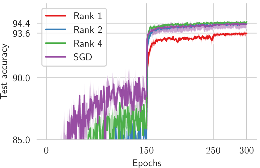
PowerSGD allows users to choose the rank of its gradient approximations. The trade-off between approximation quality and compression, decompression and transfer cost is explored in Table 3. In both the image classification and language modeling tasks we explore, the test quality achieved by PowerSGD grows with increasing rank. In both cases, it reaches a quality that is as good, or even slightly better than regular SGD.

Table 3: PowerSGD with varying rank. With sufficient rank, PowerSGD accelerates training of a ResNet18 and an LSTM by reducing communication, achieving test quality on par with regular SGD in the same number of iterations. The time per batch includes the forward/backward pass (constant). See Section 5 for the experimental setup.

Image classification — ResNet18 on Cifar10
Algorithm Test accuracy Data sent per epoch Time per batch SGD $94.3\%$ 1023 MB ($1\times$) 312 ms $+0\%$ Rank 1 $93.6\%$ 4 MB ($243\times$) 229 ms $-26\%$ Rank 2 $94.4\%$ 8 MB ($136\times$) 239 ms $-23\%$ Rank 4 $94.5\%$ 14 MB ($72\times$) 260 ms $-16\%$
Language modeling — LSTM on Wikitext-2
Algorithm Test perplexity Data sent per epoch Time per batch SGD 91 7730 MB ($1\times$) 300 ms $+0\%$ Rank 1 102 25 MB ($310\times$) 131 ms $-56\%$ Rank 2 93 38 MB ($203\times$) 141 ms $-53\%$ Rank 4 91 64 MB ($120\times$) 134 ms $-55\%$

5 Results

Default experimental setting
Dataset Cifar10 Architecture ResNet18 Number of workers 16 Backend NCCL (fastest in PyTorch) Batch size $128\times\text{number of workers}$ Momentum 0.9 Learning rate Tuned for 16 workers — $0.1\times 16$ for SGD. Scaled linearly by the number of workers LR decay $/10$ at epoch 150 and 250 LR warmup Linearly within 5 epochs, starting from the single-worker LR # Epochs 300 Weight decay $10^{-4}$, $0$ for BatchNorm parameters Repetitions 3, with varying seeds Error bars min — max

This section demonstrates the practicality of PowerSGD for distributed optimization of deep neural networks. We show that the compression scheme of PowerSGD i) is fast and matches test performance of SGD, ii) scales well with increasing workers even with a sub-optimal communication backend, and iii) significantly reduces training time for larger models.

Most of the analysis is performed on Cifar10, in the setting described in the table on the right. We verify the generality of PowerSGD by an additional evaluation of an LSTM for language modeling on Wikitext-2. We use 16 GPUs on 8 machines, connected through a fast (10Gbit/s) network. To obtain meaningful timings, we have aimed to optimize all compared optimizers to a similar level. We provide a list of our performance optimizations in Appendix H. Throughout these results, we tune the learning rate for full-precision SGD, and use the same parameters for PowerSGD and other compression algorithms that use error feedback with momentum. Learning rates for the compared-to Spectral Atomo (Wang et al., 2018) and Signum (Bernstein et al., 2019) were separately tuned cf. Appendix I.

5.1 Comparison with other compressors

Table 4: Comparing different compression operators for Error-feedback SGD in a unified setting; running 300 epochs of Error-feedback SGD with Momentum (Algorithm 2) with a learning rate tuned for full-precision SGD on 16 GPUs for Cifar10. Note that the variations of PowerSGD with ranks 2 and 7 strike the best balance between the achieved test accuracy and time per batch (total time for forward, backward, compression, decompression, and gradient aggregation).

		Test accuracy	Sent/epoch	All-reduce	Time/batch
No compression		$94.3\%$	1023 MB	✓	312 ms
Medium	Rank 7	$94.6\%$	24 MB	✓	285 ms
	Random Block	$93.3\%$	24 MB	✓	243 ms
	Random K	$94.0\%$	24 MB	✓	540 ms
	Sign+Norm	$93.9\%$	32 MB	✗	429 ms
	Top K	$94.4\%$	32 MB	✗	444 ms
High	Rank 2	$94.4\%$	8 MB	✓	239 ms
	Random Block	$87.8\%$	8 MB	✓	240 ms
	Random K	$92.6\%$	8 MB	✓	534 ms
	Top K	$93.6\%$	8 MB	✗	411 ms

Error feedback in compressed optimization enables the use of a multitude of compression schemes, including biased ones. The potential compression operators illustrated in Figure 1 are compared in Table 4. We evaluate compressors based on the test accuracy achieved and the total time taken to process one mini-batch. The former is a holistic measure of the accuracy of the compression operator, and the latter is the net time required for a forward pass, backward pass, gradient compression and decompression and gradient communication. We study two compression regimes—medium and high.

At around $32\times$ compression, achieved by sign-based methods, all compression schemes (other than Random Block) achieve test accuracy close to full-precision SGD. This implies that all schemes in this regime (other than Random Block) obtain a good-enough compression quality. At high compression ($128\times$), PowerSGD particularly stands out as the only method to achieve the target test accuracy.

In both the medium and high compression settings, the only schemes to be faster than full-precision SGD are PowerSGD and Random Block. Note that both are simple linear schemes and hence support all-reduce. While Random $K$ also supports all-reduce, the overhead for random memory access during both the compression and decompression stages is substantial, making it slower overall than SGD. Thus, on modern GPU-enabled infrastructure, PowerSGD, which relies on matrix multiplication, is faster and much more accurate than the other compression schemes.

5.2 Scalability of PowerSGD

Here we investigate how PowerSGD scales with an increasing number of workers, shedding light on what we can expect if we use a significantly larger number of workers. Additionally, we investigate how these results depend on the choice of communication backend. We benchmark PowerSGD against SGD and Signum (signSGD with majority vote) from Bernstein et al. (2019) which we believe is the current state-of-the-art for distributed algorithms.

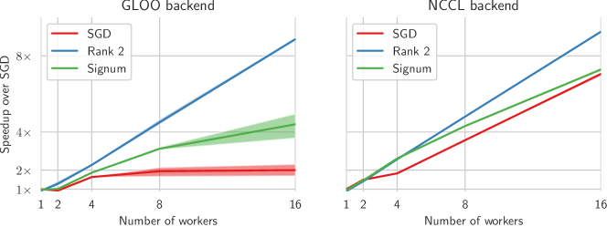
Table 5 provides a detailed breakdown of the time spent for each mini-batch (i.e. one step) into the forward pass, backward pass, gradient exchange (communication), and compression/decompression. The time spent in the forward and backward pass is constant across all algorithms and numbers of workers. Since both SGD and PowerSGD use all-reduce, the gradient communication time (solid green in Table 5) scales gracefully with increasing number of workers. Signum—which uses all-gather instead of all-reduce—has a steeper increase. It has comparable time to PowerSGD for 4 workers but becomes more expensive for 16 workers.

There is another, more subtle, consequence of all-reduce vs. all-gather on the decoding times. In all-reduce, the aggregation step and the communication step happen simultaneously. Each worker receives a pre-aggregated gradient, making the cost of decompression independent of the number of workers. On the other hand, in all-gather, a worker receives $W$ compressed gradients that need to be individually decompressed and aggregated (either using majority vote or averaging). The time for decompression with all-gather therefore scales linearly with number of workers. This shows when comparing the hatcheted regions in Table 5. This observation speaks to the importance of the reduce operation for scalability.

Table 5: Breakdown of time spent (in seconds) in one iteration of ResNet18 training. Because PowerSGD (Rank 2) uses all-reduce, time spent encoding/decoding gradients is constant.
 Forward pass,  Backward pass,  Gradient exchange,  Encoding and decoding.

	2 workers	4 workers	8 workers	16 workers
Rank 2
SGD
Signum

We next study two different backends—the more optimized NCCL  and the slower GLOO. All three methods scale reasonably well with the optimized NCCL backend, although Signum has a slope less than 1 in the log-log plot, indicating sub-linear scaling. On the slower GLOO backend, PowerSGD is notably the only method that retains excellent scaling due to its high compression rate.

Figure 3: Scaling of PowerSGD on Cifar10 compared to full-precision SGD and Signum (Bernstein et al., 2019) on two communication backends. The batch size increases linearly with the number of workers. We compare training time for one epoch to 1-worker SGD. Note that the faster NCCL backend used throughout benefits the baselines more than our method.

5.3 Other tasks and methods

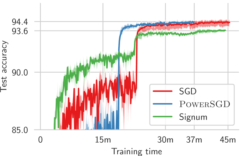
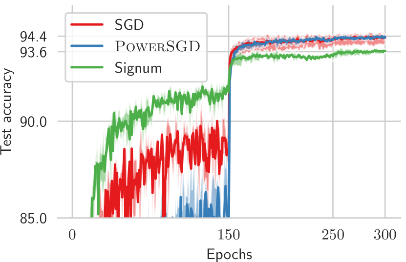
In Table 6, we compare PowerSGD against the state-of-the-art compressed optimization algorithms Signum and Spectral Atomo. The cost of performing a full SVD at each step renders Spectral Atomo impractical in a high-performance setting, especially considering that it fails to match the test accuracies of the other methods. Signum performs much better, proving a minor speedup over SGD. PowerSGD is the fastest and most accurate of the compared methods.

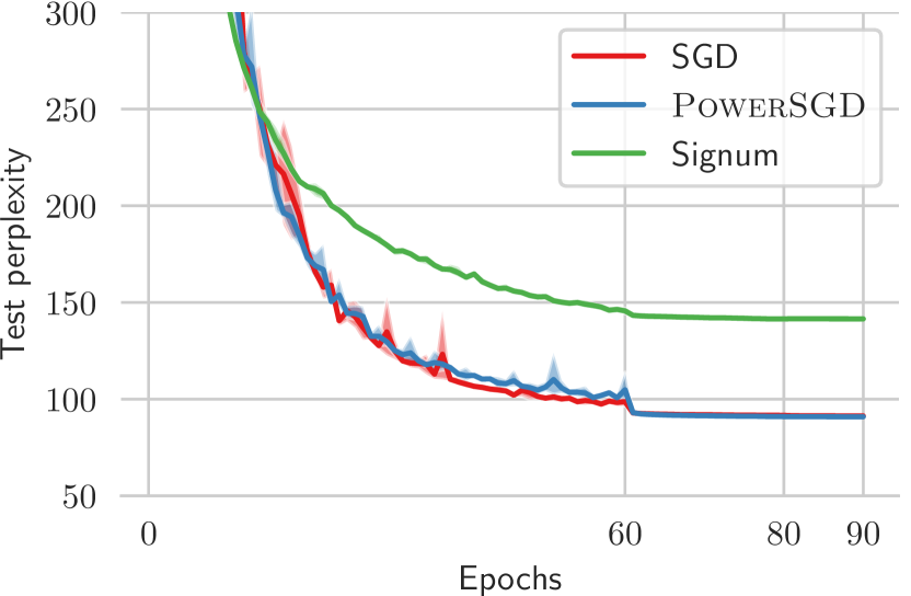
The advantage of PowerSGD truly shows when using really large models, i.e. where the communication actually becomes a bottleneck. To verify this, we run Signum, full-precision SGD, and PowerSGD to train an LSTM on a language modeling task which has a substantially larger model size than ResNet18 (see Appendix F). To match the test score of full-precision SGD, we needed to use a rank-4 approximation (see Section 4.3). PowerSGD reduces communication by $90\%$ and the overall running time by $55\%$, while Signum becomes slower than full-precision SGD and also obtains a worse test score.

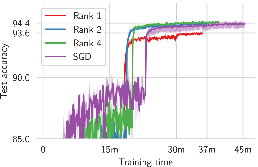
Convergence curves on test accuracy corresponding to Tables 3, 6 and 7 are provided in Appendix C. In those figures, you can read our improvements in time-to-accuracy for any target accuracy. We also provide a case study on using PowerSGD for a novel task (language modeling with transformers on Wikitext-2) and more workers (32) on the public cloud in Appendix D.

Table 6: Results on Cifar10. Contrary to rank-2 Spectral Atomo (Wang et al., 2018) and Signum (Bernstein et al., 2019), PowerSGD achieves the same test accuracy as full-precision SGD within the default epoch budget.

Algorithm	Test accuracy	Data/epoch	Time per batch
SGD	$94.3\%$	1023 MB	312 ms	$+0\%$
Atomo	$92.6\%$	113 MB	948 ms	$+204\%$
Signum	$93.6\%$	32 MB	301 ms	$-3\%$
Rank 2	$94.4\%$	8 MB	239 ms	$-23\%$

Table 7: In language modeling, rank-4 PowerSGD achieves the target test accuracy and provides a significant speedup over SGD.

Algorithm	Test perplexity	Data/epoch	Time per batch
SGD	91	7730 MB	300 ms	$+0\%$
Signum	142	242 MB	424 ms	$+41\%$
Rank 4	91	64 MB	134 ms	$-55\%$

6 Conclusion

Gradient compression is a promising approach to tackling the communication bottleneck in synchronous distributed optimization. Thus far, however, it has not found widespread adoption because existing compression schemes either run slower than SGD with optimized all-reduce gradient aggregation, or more importantly do not reach the same test performance. We see PowerSGD as the first practical gradient compression method, and believe it is ready for adaptation in practice.

The key to the practicality of PowerSGD is its linear compression scheme that is cheap to compute and allows for all-reduce gradient aggregation, while simultaneously matching the test performance of full-precision SGD. This speedup gained over SGD actually increases for larger models such as those commonly found in NLP. Further, as a result of our modifications to the error feedback algorithm, PowerSGD is a plug-in replacement for SGD with momentum, avoiding the need for additional hyper-parameter tuning. We expect that these properties of PowerSGD will enable training of even larger models with even more workers than what is possible with full-precision SGD.

While PowerSGD enables faster training with larger batch sizes, increasing batch sizes are known to eventually suffer from a ‘generalization gap’ (Shallue et al., 2018). This is an orthogonal issue that we see as the next step towards solving large-scale training. In our experiments, we have observed that PowerSGD can achieve higher test accuracy than SGD. Combined with the intriguing links between low-rankedness and generalization, this indicates that PowerSGD may also be helpful for closing the generalization gap in large batch training.

Acknowledgements

We thank Alp Yurtsever and Tao Lin for valuable discussions and the reviewers for their feedback. This project was supported by SNSF grant $200021\_175796$, as well as a Google Focused Research Award.

Appendix

Appendix A Discussion of convergence

The proof of convergence of EF-SGD with momentum can be derived by incoporating a few key changes to the proof of Karimireddy et al. (2019): i) we are in a multi-worker setting, and ii) we incorporate the techniques introduced by Ghadimi & Lan (2016) to handle the additional momentum. Further, $\lVert\cdot\rVert^{2}$ unless otherwise specified is always the standard euclidean norm for vectors, and is the Frobenius norm for matrices.

Suppose that we want to minimize a continuous (possibly) non-convex function $f\colon{}^{d}\to\real$:

$$f^{\star}=\min_{\mathbf{x}\in{}^{d}}f(\mathbf{x})\,.$$

The classic stochastic gradient algorithm (SGD) Robbins & Monro (1951) when adapted to the distributed optimization setting performs iterations of the form

$$\mathbf{x}_{t+1}:=\mathbf{x}_{t}-\gamma\,\mathbf{g}_{t}\,,\text{ where}$$ (1)

$$\mathbf{g}_{t}=\frac{1}{W}\sum_{w=1}^{W}\mathbf{g}_{t,w}\hskip 28.45274pt\text{and}\hskip 28.45274pt\operatorname{\mathbb{E}}[\mathbf{g}_{t}]=\nabla f(\mathbf{x}_{t})\,.$$

Here $\gamma\in\real$ is the step-size (or learning-rate) and $\mathbf{g}_{t,w}$ is the stochastic gradient computed by the $w$th worker for $w\in\{1,\dots,W\}$ workers.

Now EF-SGD (Algorithm 2) when run on the $W$ workers with step-size $\gamma$ and momentum parameter $\lambda$ can be rewritten making the dependence on iteration $t$ explicit as follows:

$$\begin{split}\Delta_{t}^{\prime}&=\textsc{Decompress}(\textsc{compress}(\mathbf{g}_{t}+\mathbf{e}_{t}))\,,\\ \mathbf{m}_{t+1}&=\Delta_{t}^{\prime}+\lambda\mathbf{m}_{t}\,,\\ \mathbf{x}_{t+1}&=\mathbf{x}_{t}-\gamma(\Delta_{t}^{\prime}+\mathbf{m}_{t+1})\,,\text{ and}\\ \mathbf{e}_{t+1}&=(\mathbf{g}_{t}+\mathbf{e}_{t})-\Delta_{t}^{\prime}\,.\end{split}$$ (2)

A.1 Eigen compression

Assumption A (Eigen compression).

Consider any matrix $M=g_{t}+e_{t}$ encountered during the run of Algorithm 2 such that $M$ is of rank $R$. Further, suppose that $\mathcal{C}_{r}(M)$ is the best rank-$r$ approximation of $M$ i.e.

$$\mathcal{C}_{r}(M)=\operatorname*{arg\,min}_{C}\lVert M-C\rVert^{2}\,.$$

Then we assume that there exists a $\delta_{\texttt{e},r}>0$ such that

$$\lVert M-\mathcal{C}_{r}(M)\rVert^{2}\leq(1-\delta_{\texttt{e},r})\lVert M\rVert^{2}\,\ a.s.$$

We state the below standard fact from linear algebra.

Remark 1 (Best rank-$r$ approximation).

Suppose we are given a matrix $M$ of rank $n$ whose singular value decomposition is

$$M=\sum_{i=1}^{n}\sigma_{i}\mathbf{u}_{i}\mathbf{v}_{i}^{\top}\,,$$

where the singular-values $(\sigma_{i})$ are sorted in descending order. Then the best rank-$r$ approximation of $M$ for $r\leq n$ is

$$\mathcal{C}_{r}(M)=(\sum_{i=1}^{r}\sigma_{i}\mathbf{u}_{i}\mathbf{v}_{t}^{\top})Q\,,$$

where $Q\in{}^{r\times r}$ is an orthogonal matrix, and further the quality of its approximation is bounded by

$$\lVert M-\mathcal{C}_{r}(M)\rVert^{2}=\left(1-\frac{\sum_{i=1}^{r}\sigma_{i}^{2}}{\sum_{i=1}^{n}\sigma_{i}^{2}}\right)\lVert M\rVert^{2}\,.$$

Thus if we used Algorithm 2 with exact rank-$r$ approximation of the gradients, we would converge at rate dictated by the eigen-spectrum of the gradients. If the singular values are ‘top-heavy’ i.e. the largest $r$ values are significantly larger than the rest, then a rank-$r$ approximation is quite accurate. As demonstrated in (Wang et al., 2018), the eigen-spectrum of stochastic gradients in common deep learning tasks is indeed ‘top-heavy’. Thus we can expect $\delta_{\texttt{e},r}$ to be bounded away from 0 even for very small $r$ (e.g. 1 or 2). Of course computing the actual top eigenvectors of the stochastic gradients is very computationally expensive, and more-over is not linear (and hence does not support reduce).

A.2 Subspace iteration

The key innovation in PowerSGD is to use only a single step of subspace (or power) iteration to give a fast low rank approximation (Stewart & Miller, 1975) to the given matrix, which in our case is a stochastic gradient. However, a single step of subspace iteration in general does not result in an adequate low-rank approximation of the input matrix. To combat this, and to at the same time reduce the variance of the stochastic gradient approximation compared to the full (deterministic) gradient, we propose the reuse of the low-rank approximation from the previous iteration as the starting point for the current iteration. This is in spite of the target matrices which are trying to approximate are changing, as the parameters evolve. Nevertheless, reuse here is justified because the full gradient does not change very fast (the gradient is Lipschitz by assumption) and we only perform a tiny update at each step, so can be assumed to be stationary within a small number of steps. Intuitively, by linearity of the subspace operation, the sequence of subspace steps with the reuse then is converging to the eigenvector of the averaged stochastic gradients over these steps, thus having a lower variance than the analogue without re-use, which has no such averaging effect.

For simplicity, we assume all matrices to be square and symmetric in this sub-section. These insights can be generalized to arbitrary matrices but with a substantial increase in complexity of exposition. Here, we simply note that for any non-square matrix $A$, we can instead consider

$$\tilde{A}=\begin{bmatrix}0&A\\ A^{\top}&0\end{bmatrix}$$

which is symmetric and has the same eigenvectors and eigenvalues as the original matrix $A$—see Stewart (1976) for more details on handling such cases.

We can now state an informal theorem about the convergence of subspace iteration.

Theorem I.

Suppose that we run subspace iteration as in (3) on a fixed matrix $A_{t}=M$. Also let $M=\sum_{i=1}^{n}\sigma_{i}\mathbf{u}_{i}\mathbf{u}_{i}^{\top}$ be the eigen decomposition of $M$ with $\sigma_{1}\geq\dots\sigma_{r}>\sigma_{r+1}\geq\dots\geq\sigma_{n}$. Then there exists an orthogonal matrix $Q\in{}^{r\times r}$ such that

$$\lim_{t=\infty}X_{t}=[\mathbf{u}_{1},\dots,\mathbf{u}_{r}]Q\,.$$

In other words, (3) recovers the best rank-$r$ approximation of $M$ as long as there is a gap between the $\sigma_{r}$ and $\sigma_{r+1}$ eigenvalues.

Suppose that at each iteration we receive a matrix $A_{t}\in{}^{n\times n}$ whose expectation is the same fixed matrix $M\in{}^{n\times n}$. Starting from an orthonormalized $X_{0}\in{}^{n\times r}$ (i.e. $X_{0}^{\top}X_{0}=I_{r}$), the rank-$r$ subspace iteration algorithm performs the following update:

$$X_{t+1}=\textsc{orthogonalize}(A_{t}X_{t})\,.$$ (3)

The final output of the algorithm (i.e.) the matrix approximation is $(A_{T+1}X_{T})X_{T}^{\top}$. This closely resembles the method of PowerSGD as outlines in Algorithm 1. We recommend (Arbenz, 2016) for an in-depth analysis of the (non-varying) subspace iteration algorithm.

Remark 2 (Orthogonalization is a linear operation).

We recall some more facts from linear algebra. For any square matrix $B$, there exists an orthogonal matrix $Q$ and a triangular matrix $R$ such that $QQ^{\top}=I$ and $B=QR$. This is true e.g. if we use Gram–Schmidt procedure to ortho-normalize $B$: Suppose $\textsc{orthogonalize}(B)$ uses the Gram–Schmidt procedure to orthogonalize $B$. Then there exists a triangular matrix $R$ such that

$$\textsc{orthogonalize}(B)=BR^{-1}\,.$$

Proof.

It is easy to see that for any orthogonal matrix $Q$, the matrix $[\mathbf{u}_{1},\dots,\mathbf{u}_{r}]Q$ is also orthogonal, and further is the fixed point of (3). In fact all rank-$r$ matrices which are fixed points of (3) are of this form.

We will use the observation in Remark 2 to rewrite the update (3) in a more convient fashion. There exist tringular matrices $R_{0},\dots,R_{t}$ such that

$$X_{t+1}=\textsc{orthogonalize}(A_{t}X_{t})=A_{t}X_{t}R_{t}^{-1}=(A_{t}A_{t-1}\cdots A_{0})X_{0}(R_{0}^{-1}R_{1}^{-1}\cdots R_{t}^{-1})\,.$$

Thus $X_{t+1}$ can alternatively be written as

$$X_{t+1}=\textsc{orthogonalize}((A_{t}A_{t-1}\cdots A_{0})X_{0})=\textsc{orthogonalize}(M^{t+1}X_{0})\,.$$

Here we assumed that the matrix was fixed i.e. $A_{t}=M$. Let us further assume that $X_{0}$ has a non-zero support on the first $r$ eigenvectors of $M$. Then, a gap in the eigenvalues $\sigma_{r}>\sigma_{r+1}$ implies that $\textsc{orthogonalize}(M^{t+1}X_{0})$ converges to $[\mathbf{u}_{1},\dots,\mathbf{u}_{r}]Q$. We refer to Chapter 7.2 of Arbenz (2016) for the actual proof of this fact. ∎

A.3 Single/multi worker equivalence

The difference between the update as written in (2) and Algorithm 2 is that the error computation and compression is performed on the aggregated gradient $\mathbf{g}_{t}$ instead of on the individual workers’ gradients $\mathbf{g}_{t,w}$. While in general these are not equivalent, the linearity of PowerSGD ensures that these are indeed equivalent. This implies that PowerSGD has the neat property that the algorithm is equivalent if run on $W$ workers or a single worker with a larger batch-size. This does not hold for most other schemes (e.g. sign based compression schemes, QSGD, etc.).

Lemma 3 (Equivalence of single worker and multi worker updates).

The updates in PowerSGD (i.e. Algorithm 2 using Compressor 1) are equivalent to the updates (2).

Proof.

Consider the update performed by PowerSGD for abrtiary vectors $\{\mathbf{v}_{w}\}$. Let $\mathcal{C}(\mathbf{v}_{w})$ be the compressed version of $\mathbf{v}_{w}$ for $w\in\{1,\dots,W\}$. Then by design of PowerSGD , the following holds:

$$\textsc{Decompress}(\textsc{aggregate}(\mathcal{C}(\mathbf{v}_{1}),\dots,\mathcal{C}(\mathbf{v}_{W})))=\textsc{Decompress}(\mathcal{C}(\frac{1}{W}\sum_{w}\mathbf{v}_{w}))\,.$$

This implies that running the algorithm on multiple workers, or running it on a single worker with a larger batch-size is identical. In particular,

$$\textsc{Decompress}(\textsc{aggregate}(\mathcal{C}(\mathbf{g}_{t,1}+\mathbf{e}_{t,1}),\dots,\mathcal{C}(\mathbf{g}_{t,W}+\mathbf{e}_{t,W})))$$

$$=\textsc{Decompress}(\mathcal{C}(\frac{1}{W}\sum_{w}\mathbf{g}_{t,w}+\mathbf{e}_{t,w}))$$

$$=\textsc{Decompress}(\frac{1}{W}\mathcal{C}(\mathbf{g}_{t}+\mathbf{e}_{t}))\,.$$

∎

Appendix B Cluster specifications

• 8 nodes

• GPUs: $2\times$ Nvidia GeForce GTX Titan X with 12 GB memory per node

• GPU connection: traversing PCIe and the SMP interconnect between NUMA nodes

• CPU: Intel Xeon E5-2680 v3 @ 2.50Ghz, 48 cores

• System memory: 251GiB

• Ethernet: 10Gbit/s SFI/SFP+

• Fat tree network topology

• Runing PyTorch 1.1 on Anaconda Python 3.7

Timings of collective communication operations

The figure below shows timings for the NCCL backend, which is the default in our experiments, and the GLOO backend. Note that NCCL does not support the ‘gather’ operation in PyTorchat the time of writing.

Appendix C Convergence curves

Image classification on Cifar10

Language modeling with Wikitext-2

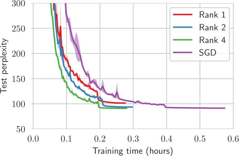
Image classification on Cifar10

Language modeling with Wikitext-2

Figure 4: Convergence curves of PowerSGD with varying rank. This figure is meant to give context to the final results and timings presented in Table 3. In two different tasks, PowerSGD with high enough rank can achieve the test quality of full-precision SGD with lower wall-clock duration. Contrary to Table 3, these timings include testing overhead at the end of each epoch, checkpointing, and other bookkeeping. Shaded areas show the min—max values over 3 replications of the experiments.

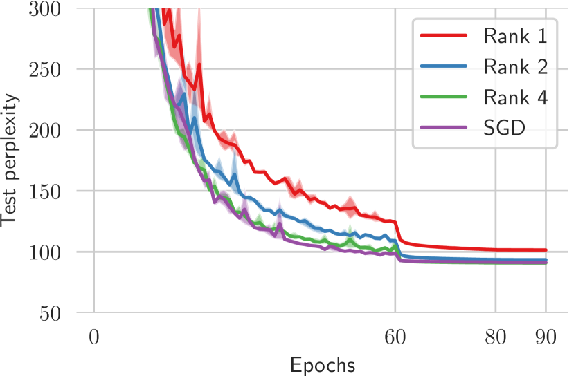
Image classification on Cifar10

Language modeling with Wikitext-2

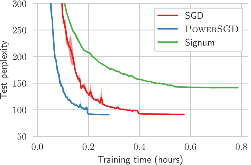
Image classification on Cifar10

Language modeling with Wikitext-2

Figure 5: Convergence curves comparing PowerSGD to the Signum optimizer Bernstein et al. (2019) (with tuned learning rate). Out of the compared methods, Signum came out as the most competitive. This figure is meant to give context to the final results and timings presented in Table 6. Contrary to Table 3, these timings include testing overhead at the end of each epoch, checkpointing, and other bookkeeping. Shaded areas show the min—max values over 3 replications of the experiments.

Appendix D Language Modeling with Transformers

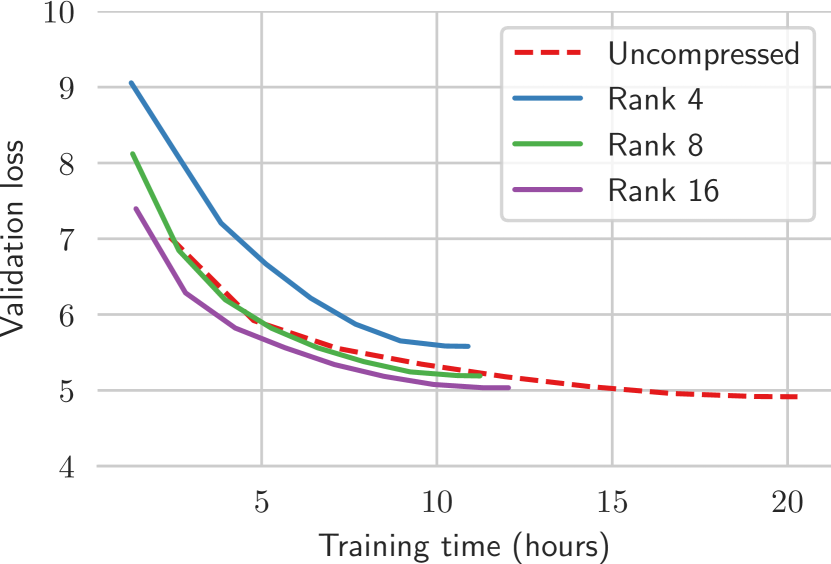
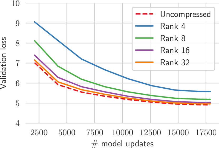
In this case study, we assess PowerSGD’s universality and ease of tuning. We implemented PowerSGD communication in Facebook AI Research’s fairseq library (Ott et al., 2019). We trained fairseq’s language modeling example with transformers (Baevski & Auli, 2019) on Google’s public cloud. The communication infrastructure, hardware, number of workers (32), and model architecture are all different from any experiments we have conducted before. See Table 8 for details.

The results of our experiments for various ranks are shown in Figure 6 and Table 9. For this task, we need a higher rank than previously (32 vs 4) to achieve a validation loss comptetitive to uncompressed SGD. We hypothesize this may be due differences in architecture to the cosine learning rate schedule. Nevertheless, even at this higher rank, we achieve a time-to-accuracy (to $\text{loss}=5$) of around $1.5\times$ and a compression ratio of $14\times$. These numbers could probably be further improved by re-tuning learning-rate-related hyperparameters.

Table 8: Experimental setting for the experiments in Appendix D

Dataset	WikiText-103
Architecture	Transformer-based (Baevski & Auli, 2019)
Framework & defaults	https://github.com/pytorch/fairseq/tree/920b85d4bd39e181229db5639c701c854c83ec5c/examples/language_model
Number of workers	32
Backend	NCCL (fastest in PyTorch)
Hardware	n1-standard-8 nodes on Google Cloud with 1 Nvidia Tesla K80 GPU
Hyperparameters	Taken from the example, not re-tuned,
	with minor changes for the higher number of workers and different GPU memory:
lr period updates	16875
max update	17875
max tokens (valid)	1536 (to fit on a K80 gpu)
tokens per sample	1536 (to fit on a K80 gpu)
warmup updates	1000
update freq	$\left[1\right]$ — don’t aggregate multiple mini-batches locally
Optimizer	original: Nesterov accelerated gradient, we just added PowerSGD for communication
Learning rate	original cosine schedule from the example
Float precision	32-bit (16-bit is unavailable on the K80)
Repetitions	1

Wall-clock time

Update steps

Figure 6: Language Modeling on Wikitext-2 with Transformers. With a large enough rank, PowerSGD can roughly match the validation loss of full-precision SGD in the same number of iterations. A speedup of $1.5\times$ in time-to-accuracy (loss=5) is achieved with a rank of 16.

Table 9: PowerSGD for Language Modeling with Transformers. With rank 32, PowerSGD achieves similar validation loss to uncompressed SGD in the same number of update steps. At this rank, the compression ratio is $14\times$ and we can train the model in 12h compared to 20h for the baseline.

Compression	Total training time		Compression ratio	Validation loss
	for 17875 updates			at 17875 updates
Uncompressed		20h	$1\times$	4.92
Rank 4		11h	$105\times$	5.58
Rank 8		11h	$55\times$	5.19
Rank 16		12h	$28\times$	5.03
Rank 32		13h	$14\times$	4.97

Forward pass    Backward pass    Gradient exchange including computation

Appendix E The need for error feedback

ResNet18 on Cifar10

Figure 7: PowerSGD with and without error feedback compared. While rank-4 PowerSGD achieves the same test accuracy as full-precision SGD, the same method without error feedback does not converge to a good accuracy at all. Both experiments use the same learning rate that was tuned for full-precision SGD.

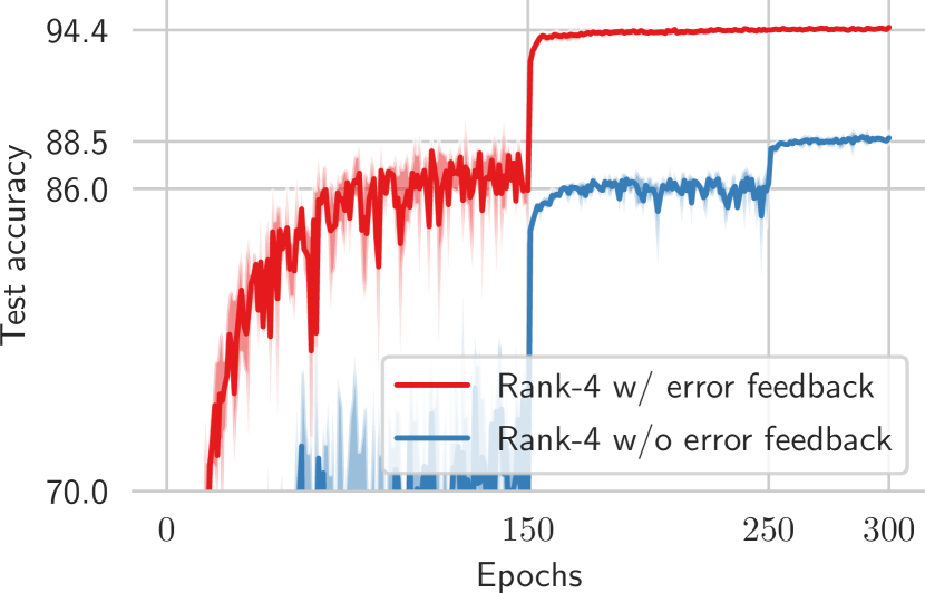
Appendix F Network parameters

See Table 10 and Table 11 for an overview of parameters in the models used.

Table 10: Parameters in the ResNet18 architecture and their shapes. The table shows the per-tensor compression ratio achieved by rank-$r$ PowerSGD.

Parameter	Gradient tensor shape	Matrix shape	Uncompressed	Compression
layer4.1.conv2	$512\times 512\times 3\times 3$	$512\times 4608$	9216 KB	$461/r\;\times$
layer4.0.conv2	$512\times 512\times 3\times 3$	$512\times 4608$	9216 KB	$461/r\;\times$
layer4.1.conv1	$512\times 512\times 3\times 3$	$512\times 4608$	9216 KB	$461/r\;\times$
layer4.0.conv1	$512\times 256\times 3\times 3$	$512\times 2304$	4608 KB	$419/r\;\times$
layer3.1.conv2	$256\times 256\times 3\times 3$	$256\times 2304$	2304 KB	$230/r\;\times$
layer3.1.conv1	$256\times 256\times 3\times 3$	$256\times 2304$	2304 KB	$230/r\;\times$
layer3.0.conv2	$256\times 256\times 3\times 3$	$256\times 2304$	2304 KB	$230/r\;\times$
layer3.0.conv1	$256\times 128\times 3\times 3$	$256\times 1152$	1152 KB	$209/r\;\times$
layer2.1.conv2	$128\times 128\times 3\times 3$	$128\times 1152$	576 KB	$115/r\;\times$
layer2.1.conv1	$128\times 128\times 3\times 3$	$128\times 1152$	576 KB	$115/r\;\times$
layer2.0.conv2	$128\times 128\times 3\times 3$	$128\times 1152$	576 KB	$115/r\;\times$
layer4.0.shortcut.0	$512\times 256\times 1\times 1$	$512\times 256$	512 KB	$171/r\;\times$
layer2.0.conv1	$128\times 64\times 3\times 3$	$128\times 576$	288 KB	$105/r\;\times$
layer1.1.conv1	$64\times 64\times 3\times 3$	$64\times 576$	144 KB	$58/r\;\times$
layer1.1.conv2	$64\times 64\times 3\times 3$	$64\times 576$	144 KB	$58/r\;\times$
layer1.0.conv2	$64\times 64\times 3\times 3$	$64\times 576$	144 KB	$58/r\;\times$
layer1.0.conv1	$64\times 64\times 3\times 3$	$64\times 576$	144 KB	$58/r\;\times$
layer3.0.shortcut.0	$256\times 128\times 1\times 1$	$256\times 128$	128 KB	$85/r\;\times$
layer2.0.shortcut.0	$128\times 64\times 1\times 1$	$128\times 64$	32 KB	$43/r\;\times$
linear	$10\times 512$	$10\times 512$	20 KB	$10/r\;\times$
conv1	$64\times 3\times 3\times 3$	$64\times 27$	7 KB	$19/r\;\times$
Bias vectors (total)			38 KB	None
Total			43 MB	$243/r\;\times$

Table 11: Parameters in the LSTM architecture and their shapes. The table shows the per-tensor compression ratio achieved by rank-$r$ PowerSGD.

Parameter	Gradient tensor shape	Matrix shape	Uncompressed	Compression
encoder	$28869\times 650$	$28869\times 650$	73300 KB	$636/r\;\times$
rnn-ih-l0	$2600\times 650$	$2600\times 650$	6602 KB	$520/r\;\times$
rnn-hh-l0	$2600\times 650$	$2600\times 650$	6602 KB	$520/r\;\times$
rnn-ih-l1	$2600\times 650$	$2600\times 650$	6602 KB	$520/r\;\times$
rnn-hh-l1	$2600\times 650$	$2600\times 650$	6602 KB	$520/r\;\times$
rnn-ih-l2	$2600\times 650$	$2600\times 650$	6602 KB	$520/r\;\times$
rnn-hh-l2	$2600\times 650$	$2600\times 650$	6602 KB	$520/r\;\times$
Bias vectors (total)			174 KB	None
Total			110 MB	$310/r\;\times$

Appendix G Compressor implementation details

G.1 Random Block

This implements compression for error-feedback with momentum (Algorithm 2).

Algorithm 3 Random Block compression

1:function compress(update matrix $M\in\mathbb{R}^{n\times m}$)

2:     Treat $M$ as a vector of length $nm$.

3:     Sample an index $s$ uniformly between 0 and $nm-1$, using the same seed on all workers.

4:     The block length $b$ is set to $(m+n)r$ to match rank-$r$ PowerSGD.

5:     return A consequtive memory slice $S=M(s:s+b)$.

6:end function

7:function aggregate+decompress(worker’s slices $S_{1}\ldots S_{W}$)

8:     $\hat{M}\leftarrow\mathbf{0}\in\mathbb{R}^{n\times m}$

9:     $\hat{M}(s:s+b)\leftarrow\frac{1}{W}\sum_{i=1}^{W}S_{i}$ $\triangleright$ using all-reduce

10:     return $\hat{M}$

11:end function

G.2 Random K

This implements compression for error-feedback with momentum (Algorithm 2).

Algorithm 4 Random $K$ compression

1:function compress(update matrix $M\in\mathbb{R}^{n\times m}$)

2:     Treat $M$ as a vector of length $nm$.

3:     The number of samples $b$ is set to $(m+n)r$ to match rank-$r$ PowerSGD.

4:     Sample a set of $b$ indices $I$ without replacement, using the same seed on all workers.

5:     return Looked up values $S=M(I)$.

6:end function

7:function aggregate+decompress(worker’s values $S_{1}\ldots S_{W}$)

8:     $\hat{M}\leftarrow\mathbf{0}\in\mathbb{R}^{n\times m}$

9:     $\hat{M}(I)\leftarrow\frac{1}{W}\sum_{i=1}^{W}S_{i}$ $\triangleright$ using all-reduce

10:     return $\hat{M}$

11:end function

Sampling of indices

We sample random indices on the CPU using Numpy. This operation is relatively expensive. Together with the many random lookups, this explains why Random $K$ compression is significantly slower than Random Block compression.

G.3 Sign+Norm

This implements compression for error-feedback with momentum (Algorithm 2).

Algorithm 5 Sign$+$Norm compression

1:function compress(update matrix $M\in\mathbb{R}^{n\times m}$)

2:     Compute the signs $S\in\left\{-1,1\right\}^{n\times m}$ of $M$

3:     Compute the $L_{1}$ norm $\ell$ of $M$.

4:     return ($\ell$, $S$)

5:end function

6:function aggregate+decompress(worker’s norms $\ell_{1}\ldots\ell_{W}$ and signs $S_{1}\ldots S_{W}$)

7:     return $\frac{1}{W}\sum_{i=1}^{W}\frac{\ell_{i}}{nm}S_{i}$ $\triangleright$ Executed on all workers using NCCL’s all-gather

8:end function

Because PyTorch does not natively support data types smaller than 8 bits per scalar, we use a C++ extension (Bernstein et al., 2019) to actually send single bits to other workers. The employed all-gather operation from NCCL is faster than aggregation using a parameter server using GLOO. We cannot implement a parameter server in NCCL due to lack of a ‘gather’ operation.

G.4 Top K

This implements compression for error-feedback with momentum (Algorithm 2).

Algorithm 6 Top $K$ compression

1:function compress(update matrix $M\in\mathbb{R}^{n\times m}$)

2:     Treat $M$ as a vector of length $nm$.

3:     The number of samples $b$ is set to $(m+n)r$ to match rank-$r$ PowerSGD.

4:     Construct a list of $b$ indices $I$ corresponding to the top absolute values in $M$.

5:     return Looked up values $S=M(I)$ and indices $I$.

6:end function

7:function aggregate+decompress(worker’s values $S_{1}\ldots S_{W}$ and indices $I_{1}\ldots I_{W}$)

8:     $\hat{M}\leftarrow\mathbf{0}\in\mathbb{R}^{n\times m}$

9:     for worker index $i$ in $1,\ldots,W$ do

10:         $\hat{M}(I_{i})\leftarrow\frac{1}{W}S_{i}$ $\triangleright$ using all-gather in NCCL

11:     end for

12:     return $\hat{M}$

13:end function

The employed all-gather operation from NCCL is faster than aggregation using a parameter server using GLOO. We cannot implement a parameter server in NCCL due to lack of a ‘gather’ operation.

G.5 Signum

This is our implementation of the Signum compression algorithm by Bernstein et al. (2019). We run it in its original form, without error feedback, with momentum of 0.9, and a learning rate tuned based on 5 experiments in the 16-worker setting.

Algorithm 7 Signum compression

1:function compress(update matrix $M\in\mathbb{R}^{n\times m}$)

2:     Compute the signs $S\in\left\{-1,1\right\}^{n\times m}$ of $M$

3:     return $S$

4:end function

5:function aggregate+decompress(worker’s signs $S_{1}\ldots S_{W}$)

6:     return $\textsc{sign}(\sum_{i=1}^{W}S_{i})$ $\triangleright$ Majority vote, on all workers using NCCL’s all-gather

7:end function

Because PyTorch does not natively support data types smaller than 8 bits per number, we use a C++ extension Zhao (2019) to actually send single bits to other workers. The employed all-gather operation from NCCL is faster than aggregation using a parameter server using GLOO. We cannot implement a parameter server in NCCL due to lack of a ‘gather’ operation.

G.6 Atomo

This is our implementation of the Spectral Atomo algorithm presented by Wang et al. (2018). We run it in its original form, without error feedback, with momentum of 0.9, and a learning rate tuned based on 4 experiments in the 16-worker setting.

Matix shape

Atomo differs from PowerSGD in how it treats tensors as matrices. This results in lower compression at the same rank.

Number of sampled components

Atomo decomposes gradient matrices $M$ using a Singular Value Decomposition into $M\sim\sum_{i}U_{i:}S_{ii}V_{i:}^{\top}$ and importance-samples components from this summation based on probabilities derived from the absolute singular values $S_{ii}$. The probabilities are such, that the expected number of samples components is equal to the target rank $r$, but there is no guarantee. We modify the algorithm to always use exactly $r$ components, to allow for faster communication. We achieve this by repeating the sampling procedure until the number of selected components is $r$. This has no significant impact on the runtime performance.

Algorithm 8 Rank-$r$ Spectral-Atomo compression

1:function compress(update matrix $M\in\mathbb{R}^{n\times m}$)

2:     $U,S,V\leftarrow\textsc{svd}(M)$. $\triangleright$ on CPU using Numpy, faster than PyTorch

3:     Compute Atomo probabilities $p_{1}\ldots p_{k}$ from $S_{11},\ldots S_{kk}$. $\triangleright$ see Wang et al. (2018).

4:     Sampling: include index $i$ independently with probability $p_{i}$.

5:     Repeat sampling until a set of $r$ indices $C$ is selected. $\triangleright$ our modification (see above)

6:     return $\left\{(U_{i:}\cdot S_{ii}/p_{i},V_{i:})\;|\;i\in C\right\}$ as two matrices $U^{\prime}\in\mathbb{R}^{n\times r}$ and $V^{\prime}\in\mathbb{R}^{m\times r}$.

7:end function

8:function aggregate+decompress(rank-$r$ approximations $(U^{\prime}_{1},V^{\prime}_{1})\ldots(U^{\prime}_{W},V^{\prime}_{W})$ for each worker)

9:     return $\sum_{i=1}^{W}U^{\prime}_{i}V_{i}^{\prime\top}$ $\triangleright$ using all-gather in NCCL

10:end function

The employed all-gather operation from NCCL is faster than aggregation using a parameter server using GLOO. We cannot implement a parameter server in NCCL due to lack of a ‘gather’ operation.

G.7 Best-approximation PowerSGD

This variant is the same as PowerSGD (Algorithm 1), but with more steps of subspace iteration, and without reuse of previous steps. We find that 4 steps of subspace iterations (8 matrix multiplications) is enough to converge to the best low-rank approximation of gradient matrices, when measuring final test accuracy achieved by PowerSGD.

Appendix H Performance optimizations

Because we compare timings, we have aimed to optimize all compared optimizers to a similar level. For sign-based methods, we used a publicly available C++ library by Bernstein et al. (2019) to efficiently pack the signs into bitmaps, an operation which is not supported by PyTorch natively. For Atomo, we have benchmarked the SVD operation on the GPU and CPU, and chose the faster CPU implementation. For all methods, we pack all gradient tensors into one flat buffer to reduce the number of communications. Where possible, we overlay communication with computation. Algorithms that do not support all-reduce are implemented using NCCL’s all-gather, which is faster than a parameter server with GLOO.

Appendix I Learning rate tuning

For each task and each optimization algorithm without error feedback, learning rates were tuned separately. For algorithms based on error feedback with momentum, we use the learning rate tuned for SGD.

Learning rates are defined as rates for 1 worker, and scaled linearly with 5-epoch warmup to the number of workers (16 by default). We tune them in the 16-worker setting.

We determine the best learning rate by comparing test accuracy of one replication after running the full number of epochs. We start training with 3 different learning rates, a factor 2 apart, based on commonly used rates for the optimizer, and if the best learning rate is either the lower or higher end, we extended the range.

For Cifar10, the rates considered for SGD were [0.05, 0.1, 0.2], we chose 0.1. For rank-2 Spectral Atomo, we considered [0.025, 0.05, 0.1, 0.2] and chose 0.1. For Signum, we considered [2e-5, 5e-5, 1e-4, 2e-4] and chose 5e-5.

For Wikitext-2, the rates considered for SGD were [0.6, 1.25, 2.5, 5, 10], we chose 1.25. For Signum, we considered [2e-4, 1e-1, 5e-5, 1e-5, 1e-6], and chose 1e-5.

We have not tuned the momentum parameter or $L_{2}$, weight decay parameters or learning rate schedule for any experiment.

References

- Alistarh et al. (2017) Alistarh, D., Grubic, D., Li, J., Tomioka, R., and Vojnovic, M. QSGD: Communication-efficient sgd via gradient quantization and encoding. In Advances in Neural Information Processing Systems (NIPS), 2017.
- Arbenz (2016) Arbenz, P. Lecture notes on solving large scale eigenvalue problems. D-MATH, ETH Zürich, 2, 2016.
- Arora et al. (2018) Arora, S., Ge, R., Neyshabur, B., and Zhang, Y. Stronger generalization bounds for deep nets via a compression approach. In International Conference on Machine Learning (ICML), 2018.
- Awan et al. (2018) Awan, A. A., Chu, C.-H., Subramoni, H., and Panda, D. K. Optimized broadcast for deep learning workloads on dense-GPU infiniband clusters: MPI or NCCL? In European MPI Users’ Group Meeting (EuroMPI), 2018.
- Baevski & Auli (2019) Baevski, A. and Auli, M. Adaptive input representations for neural language modeling. In International Conference on Learning Representations (ICLR), 2019.
- Bernstein et al. (2018) Bernstein, J., Wang, Y.-X., Azizzadenesheli, K., and Anandkumar, A. signSGD: compressed optimisation for non-convex problems. In International Conference on Machine Learning (ICML), 2018.
- Bernstein et al. (2019) Bernstein, J., Zhao, J., Azizzadenesheli, K., and Anandkumar, A. signSGD with majority vote is communication efficient and fault tolerant. In International Conference on Learning Representations (ICLR), 2019.
- Caldas et al. (2018) Caldas, S., Konecný, J., McMahan, H. B., and Talwalkar, A. Expanding the reach of federated learning by reducing client resource requirements. arXiv, abs/1812.07210, 2018.
- Carlson et al. (2015) Carlson, D., Cevher, V., and Carin, L. Stochastic Spectral Descent for Restricted Boltzmann Machines. In International Conference on Artificial Intelligence and Statistics (AISTATS), 2015.
- Collins et al. (2018) Collins, E., Bigdeli, S. A., and Süsstrunk, S. Detecting memorization in ReLU networks. arXiv, abs/1810.03372, 2018.
- Dean et al. (2012) Dean, J., Corrado, G., Monga, R., Chen, K., Devin, M., Mao, M., Senior, A., Tucker, P., Yang, K., Le, Q. V., et al. Large scale distributed deep networks. In Advances in Neural Information Processing Systems (NIPS), 2012.
- Ghadimi & Lan (2016) Ghadimi, S. and Lan, G. Accelerated gradient methods for nonconvex nonlinear and stochastic programming. Mathematical Programming, 156(1-2):59–99, 2016.
- Goyal et al. (2017) Goyal, P., Dollar, P., Girshick, R., Noordhuis, P., Wesolowski, L., Kyrola, A., Tulloch, A., Jia, Y., and He, K. Accurate, large minibatch SGD: training imagenet in 1 hour. arXiv, abs/1706.02677, 2017.
- Gunasekar et al. (2018) Gunasekar, S., Lee, J., Soudry, D., and Srebro, N. Characterizing implicit bias in terms of optimization geometry. In International Conference on Machine Learning (ICML), 2018.
- Iandola et al. (2015) Iandola, F. N., Ashraf, K., Moskewicz, M. W., and Keutzer, K. FireCaffe: near-linear acceleration of deep neural network training on compute clusters. corr abs/1511.00175 (2015), 2015.
- Karimireddy et al. (2019) Karimireddy, S. P., Rebjock, Q., Stich, S. U., and Jaggi, M. Error feedback fixes SignSGD and other gradient compression schemes. In International Conference on Machine Learning (ICML), 2019.
- Konečnỳ et al. (2016) Konečnỳ, J., McMahan, H. B., Yu, F. X., Richtárik, P., Suresh, A. T., and Bacon, D. Federated learning: Strategies for improving communication efficiency. arXiv, abs/1610.05492, 2016.
- Li et al. (2018) Li, Y., Ma, T., and Zhang, H. Algorithmic regularization in over-parameterized matrix sensing and neural networks with quadratic activations. In Conference on Learning Theory (COLT), 2018.
- Lin et al. (2018) Lin, Y., Han, S., Mao, H., Wang, Y., and Dally, W. J. Deep gradient compression: Reducing the communication bandwidth for distributed training. In International Conference on Learning Representations (ICLR), 2018.
- Martin & Mahoney (2018) Martin, C. H. and Mahoney, M. W. Implicit self-regularization in deep neural networks: Evidence from random matrix theory and implications for learning. arXiv, abs/1810.01075, 2018.
- Mazumder et al. (2010) Mazumder, R., Hastie, T., and Tibshirani, R. Spectral regularization algorithms for learning large incomplete matrices. Journal of Machine Learning Research, 11(Aug):2287–2322, 2010.
- Oja (1982) Oja, E. Simplified neuron model as a principal component analyzer. Journal of Mathematical Biology, 15(3):267–273, 1982.
- Ott et al. (2019) Ott, M., Edunov, S., Baevski, A., Fan, A., Gross, S., Ng, N., Grangier, D., and Auli, M. fairseq: A fast, extensible toolkit for sequence modeling. In Proceedings of NAACL-HLT 2019: Demonstrations, 2019.
- Panda et al. (2019) Panda, D. K. D., Subramoni, H., and Awan, A. A. High performance distributed deep learning: A beginner’s guide. In Symposium on Principles and Practice of Parallel Programming (PPoPP), 2019.
- Robbins & Monro (1951) Robbins, H. and Monro, S. A Stochastic Approximation Method. The Annals of Mathematical Statistics, 22(3):400–407, September 1951.
- Seide et al. (2014) Seide, F., Fu, H., Droppo, J., Li, G., and Yu, D. 1-bit stochastic gradient descent and its application to data-parallel distributed training of speech dnns. In Annual Conference of the International Speech Communication Association (INTERSPEECH), 2014.
- Shallue et al. (2018) Shallue, C. J., Lee, J., Antognini, J., Sohl-Dickstein, J., Frostig, R., and Dahl, G. E. Measuring the effects of data parallelism on neural network training. arXiv, abs/1811.03600, 2018.
- Stewart (1976) Stewart, G. Simultaneous iteration for computing invariant subspaces of non-Hermitian matrices. Numerische Mathematik, 25(2):123–136, 1976.
- Stewart & Miller (1975) Stewart, G. and Miller, J. Methods of simultaneous iteration for calculating eigenvectors of matrices. Topics in Numerical Analysis II, pp. 169–185, 1975.
- Stich & Karimireddy (2019) Stich, S. U. and Karimireddy, S. P. The error-feedback framework: Better rates for sgd with delayed gradients and compressed communication. arXiv, abs/1909.05350, 2019.
- Stich et al. (2018) Stich, S. U., Cordonnier, J.-B., and Jaggi, M. Sparsified SGD with memory. In Advances in Neural Information Processing Systems (NeurIPS), 2018.
- Wang et al. (2018) Wang, H., Sievert, S., Liu, S., Charles, Z., Papailiopoulos, D., and Wright, S. ATOMO: Communication-efficient learning via atomic sparsification. In Advances in Neural Information Processing Systems (NeurIPS), 2018.
- Wangni et al. (2018) Wangni, J., Wang, J., Liu, J., and Zhang, T. Gradient sparsification for communication-efficient distributed optimization. In Advances in Neural Information Processing Systems (NeurIPS), 2018.
- Wen et al. (2017) Wen, W., Xu, C., Yan, F., Wu, C., Wang, Y., Chen, Y., and Li, H. Terngrad: Ternary gradients to reduce communication in distributed deep learning. In Advances in Neural Information Processing Systems (NIPS), pp. 1509–1519, 2017.
- Yoshida & Miyato (2017) Yoshida, Y. and Miyato, T. Spectral norm regularization for improving the generalizability of deep learning. arXiv, abs/1705.10941, 2017.
- Yu et al. (2018) Yu, M., Lin, Z., Narra, K., Li, S., Li, Y., Kim, N. S., Schwing, A. G., Annavaram, M., and Avestimehr, S. Gradiveq: Vector quantization for bandwidth-efficient gradient aggregation in distributed CNN training. In Advances in Neural Information Processing Systems (NeurIPS), 2018.
- Yurtsever et al. (2017) Yurtsever, A., Udell, M., Tropp, J. A., and Cevher, V. Sketchy decisions: Convex low-rank matrix optimization with optimal storage. In International Conference on Artificial Intelligence and Statistics (AISTATS), 2017.
- Zhao (2019) Zhao, J. signSGD with majority vote. github.com/PermiJW/signSGD-with-Majority-Vote, 2019. [Online; accessed 12-May-2019].