On approximate solutions of the equations of incompressible magnetohydrodynamics

Livio Pizzocchero$\,{}^{a}$ (), Emanuele Tassi $\,{}^{b,c}$
^a Dipartimento di Matematica, Università di Milano

Via C. Saldini 50, I-20133 Milano, Italy

and Istituto Nazionale di Fisica Nucleare, Sezione di Milano, Italy

e–mail: livio.pizzocchero@unimi.it

^b Aix Marseille Univ, Univ Toulon, CNRS, CPT, Marseille, France

^c Université Côte d’Azur, Observatoire de la Côte d’Azur, CNRS,

Laboratoire Lagrange, France

e–mail: etassi@oca.eu

Inspired by an approach proposed previously for the incompressible Navier-Stokes (NS) equations, we present a general framework for the a posteriori analysis of the equations of incompressible magnetohydrodynamics (MHD) on a torus of arbitrary dimension $d$; this setting involves a Sobolev space of infinite order, made of $C^{\infty}$ vector fields (with vanishing divergence and mean) on the torus. Given any approximate solution of the MHD Cauchy problem, its a posteriori analysis with the method of the present work allows to infer a lower bound on the time of existence of the exact solution, and to bound from above the Sobolev distance of any order between the exact and the approximate solution. In certain cases the above mentioned lower bound on the time of existence is found to be infinite, so one infers the global existence of the exact MHD solution. We present some applications of this general scheme; the most sophisticated one lives in dimension $d=3$, with the ABC flow (perturbed magnetically) as an initial datum, and uses for the Cauchy problem a Galerkin approximate solution in $124$ Fourier modes. We illustrate the conclusions arising in this case from the a posteriori analysis of the Galerkin approximant; these include the derivation of global existence of the exact MHD solution with the ABC datum, when the dimensionless viscosity and resistivity are equal and stay above an explicitly given threshold value.

Keywords: Magnetohydrodynamics, existence and regularity theory, theoretical approximation, a posteriori analysis.

AMS 2000 Subject classifications: 35Q35, 76W05.

1 Introduction

Magnetohydrodynamics (MHD) and the Navier-Stokes (NS) equations. The incompressible MHD equations are usually written as follows (in dimensionless form):

$$\dot{u}=\nu\Delta u-u{\scriptstyle{\bullet}}\partial u+b{\scriptstyle{\bullet}}\partial b-\partial(p+{1\over 2}|b|^{2})~{},$$ (1.1)

$$\dot{b}=\eta\Delta b-u{\scriptstyle{\bullet}}\partial b+b{\scriptstyle{\bullet}}\partial u~{},$$ (1.2)

$$\mbox{div}u=0~{},\quad\mbox{div}b=0~{}.$$ (1.3)

Here: $u=u(x,t)$ and $b=b(x,t)$ are, respectively, the velocity and magnetic field, depending on the space variables $x=(x_{1},...,x_{d})$ and on time $t$, whereas $p=p(x,t)$ is the pressure; the constants $\nu,\eta\geqslant 0$ are the viscosity and resistivity. Throughout the paper we consider periodic boundary conditions, or, more precisely, we assume $x$ to range in the $d$-dimensional torus ${{\mathbb{T}}}^{d}:=({\mathbb{R}}/2\pi{\mathbb{Z}})^{d}$. Thus $u,b:{{\mathbb{T}}}^{d}\times[0,T)\rightarrow{\mathbb{R}}^{d}$ (and $p:{{\mathbb{T}}}^{d}\times[0,T)\rightarrow{\mathbb{R}}$). In Eqs. (1.1) (1.2) and in the rest of the paper, $\partial$ stands for the gradient and, for all (sufficiently regular) vector fields $v,w$, we indicate with $v{\scriptstyle{\bullet}}\partial w$ the vector field with components $(v{\scriptstyle{\bullet}}\partial w)_{r}:=\sum_{s=1}^{d}v_{s}\partial_{s}w_{r}$; of course $\Delta:=\sum_{r=1}^{d}\partial_{rr}$ is the Laplacian. The space dimension $d$ is arbitrary, but we are typically interested in the case $d=3$. For $d=3$, one can write the above equations in a more familiar form using the identities $-u{\scriptstyle{\bullet}}\partial b+b{\scriptstyle{\bullet}}\partial u=\mbox{rot}(u\wedge b)$ and $b{\scriptstyle{\bullet}}\partial b-\partial(|b|^{2}/2)=(\mbox{rot}\,b)\wedge b$ (the first one holding for all divergence free vector fields $u,b$ and the second one valid for any vector field $b$).

One can reexpress Eqs. (1.1) (1.2) applying to both sides the Leray projection $\mathcal{L}$, which transforms any vector field (on the torus) into its divergence free part; this operator annihilates gradients, so that Eqs. (1.1) (1.2) become

$$\dot{u}=\nu\Delta u-\mathcal{L}(u{\scriptstyle{\bullet}}\partial u)+\mathcal{L}(b{\scriptstyle{\bullet}}\partial b)~{},$$ (1.4)

$$\dot{b}=\eta\Delta b-\mathcal{L}(u{\scriptstyle{\bullet}}\partial b)+\mathcal{L}(b{\scriptstyle{\bullet}}\partial u)~{},$$ (1.5)

(and no longer contain the pressure $p$). It should be noted that the vector field $-u{\scriptstyle{\bullet}}\partial b+b{\scriptstyle{\bullet}}\partial u$ is divergence free like $u$ and $b$, so that $-\mathcal{L}(u{\scriptstyle{\bullet}}\partial b)+\mathcal{L}(b{\scriptstyle{\bullet}}\partial u)=-u{\scriptstyle{\bullet}}\partial b+b{\scriptstyle{\bullet}}\partial u$. In spite of this, for our purposes it is convenient to indicate explicitly $\mathcal{L}$ in these terms of Eq. (1.5); one advantage is that, in this formulation, all bilinear terms in Eqs. (1.4) (1.5) involve a unique bilinear map

$${\mathscr{P}}:(v,w)\mapsto{\mathscr{P}}(v,w):=-\mathcal{L}(v{\scriptstyle{\bullet}}\partial w)$$ (1.6)

(where $v,w:{{\mathbb{T}}}^{d}\rightarrow{\mathbb{R}}^{d}$ are any two sufficiently smooth vector fields). This “fundamental” bilinear map is the same governing the NS equations of incompressible fluids, which read

$$\dot{u}=\nu\Delta u+{\mathscr{P}}(u,u)$$ (1.7)

(with $u$ representing again the velocity field, and $\nu\geqslant 0$ the viscosity; for $\nu=0$, these become the Euler equations). A posteriori analysis of NS approximate solutions: a review of known results. The structural analogies between the MHD equations (1.4)(1.5) and the NS equations (1.7) suggest the possibility to extend to the MHD case an approach developed in the last years for the NS equations, allowing to infer rigorous results on their exact solutions from the a posteriori analysis of approximate solutions. This a posteriori approach to the NS equations was started in [1] [2] [3] and continued in a series of papers co-authored by one of us [4] [5] [6] [7]; there are close relations between this scheme and a strategy proposed for other nonlinear PDEs (especially, the equations of surface growth), which has even been extended to stochastic PDEs [8] [9] [10] [11].

Let us give some more information about [4] [5] [6] [7]; here one works in a rigorous functional setting, where the exact or approximate solutions of the NS Cauchy problem take values in suitable Sobolev spaces of (divergence free, mean zero) vector fields on the torus ${{\mathbb{T}}}^{d}$. These Sobolev spaces are based on $L^{2}$, and their order is either finite [4] or infinite [7]; the case of infinite order amounts to work in a space of $C^{\infty}$ vector fields. In this framework one considers an approximate solution of the NS Cauchy problem, i.e., a function fulfilling the NS equations with a given initial datum up to errors affecting both the evolution equations and the initial condition. Setting up an a posteriori analysis centered about the Sobolev norms of the above errors, one obtains a lower bound on the time of existence of the exact solution of the NS Cauchy problem, and also derives upper bounds on the Sobolev distances between the exact and the approximate solution at any instant. The previously mentioned lower bound on the time of existence of the NS solution can be $+\infty$; in this case, one concludes that the solution of the NS Cauchy problem is defined on the whole interval $[0,+\infty)$, i.e., it is global.

The key ingredient in the above constructions are certain differential inequalities supplemented with suitable “initial value inequalities”, built up from the norms of the errors mentioned previously; these are referred to as the control inequalities. The unknowns in these inequalities are real valued functions of time; there is a pair of control inequalities (a differential and an initial value inequality) for any Sobolev order, and a solution is an upper bound on the Sobolev distance of that order between the exact and the approximate NS solution. The time of existence of a solution of the control inequalities of some basic Sobolev order also gives a lower bound on the time of existence for the exact solution of the NS Cauchy problem. The simplest way to solve a pair of control inequalities is to fulfill them as equalities: in this case we have a differential equation and an initial condition for an unknown real function of time, forming what we call a control Cauchy problem and possessing a unique solution.

In the applications already proposed for the above scheme, the approximate NS solutions are obtained using the Galerkin method [4] or a truncated expansion with respect to a suitable quantity, which can be the reciprocal of the viscosity [5] or the time variable [6]. The fully quantitative implementation of the a posteriori analysis requires accurate estimates on the constants in certain inequalities about the fundamental bilinear map (1.6), involving the Sobolev norms; rather accurate upper bounds on these constants have been given in [12] [13] [14]. Contents of the present work. The aim of this paper is to transfer some results on the NS equations to the MHD case; these results concern mainly the a posteriori analysis of approximate solutions, as developed in [7] (and in the previous work [4]) for NS equations.

The key point in our constructions is a formulation of the MHD equations, emphasizing strong analogies with the setting of [7] for NS equations. In few words, the pair of functions $\mathbf{u}:=(u,b)$ appearing in the MHD equations (1.4) (1.5) is viewed as taking values in the product of two copies of an infinite order Sobolev space (made of divergence free and mean zero vector fields on ${{\mathbb{T}}}^{d}$), and the cited equations are written as

$$\dot{\mathbf{u}}={\mbox{\boldmath$\mathscr{A}$}}\mathbf{u}+{\mbox{\boldmath$\mathscr{P}$}}(\mathbf{u},\mathbf{u})~{};$$ (1.8)

here $\mathscr{A}$ is the operator $(u,b)$ $\mapsto$ $(\nu\Delta u,\eta\Delta b)$ and $\mathscr{P}$ is a “two component” bilinear map whose definition is suggested by the structure of the bilinear terms in Eqs. (1.4) (1.5) (see Eq. (3.8) for the necessary details). One can notice that the NS equations (1.7) are formally converted into the MHD equations (1.8) with the substitutions

$$u\rightsquigarrow\mathbf{u},\quad\nu\Delta\rightsquigarrow{\mbox{\boldmath$\mathscr{A}$}},\quad{\mathscr{P}}\rightsquigarrow{\mbox{\boldmath$\mathscr{P}$}}~{}.$$ (1.9)

These structural similarities are very deep. In fact, as shown in the present paper, some important Sobolev norm inequalities fulfilled by the NS bilinear map ${\mathscr{P}}$ have essentially identical counterparts for $\mathscr{P}$; this is a not-so-trivial fact, whose proof requires a minimum of effort. In addition, some Sobolev norm inequalities for $\nu\Delta$ have counterparts for $\mathscr{A}$, based on the parameter $\mu:=\min(\nu,\eta)$.

After pointing out the above structural analogies, in the present work we consider any approximate solution of the MHD Cauchy problem and we analyze it a posteriori, using ideas developed in [7] for the NS equations and adapting them to the MHD case. In this way we derive lower bounds on the time of existence of the exact MHD solution and upper bounds on the Sobolev distances (of any order) between the exact and the approximate solution; suitable control inequalities (conceptually similar to those mentioned in the previous paragraph) are developed for this purpose. In some cases, this construction ensures the global existence in time (i.e., a domain $[0,+\infty)$) for the exact solution of the MHD Cauchy problem.

Some basic estimates on the exact solution of the MHD Cauchy problem can be obtained applying the previous scheme to a very simple approximate solution, namely, the zero function. The a posteriori analysis of the zero function shows, amongst else, that the solution of the MHD Cauchy problem with any smooth initial datum is global if $\mu:=\min(\nu,\eta)$ is above a computable threshold value, depending on the datum. As examples we present these basic estimates in space dimension $d=3$, choosing as initial data the Orszag-Tang vortex and an Arnold-Beltrami-Childress (ABC) flow with a perturbing magnetic field [15] [16].

A second, more sophisticated application is developed subsequently; this uses an approximate solution provided by the Galerkin method (i.e., by the truncation of the MHD equations to a finite set of Fourier modes). For this construction we take inspiration from the Galerkin method for NS equations, in the approach described by [4].

The explicit (numerical) construction of the Galerkin approximants for the MHD Cauchy problem is exemplified in space dimension $d=3$, assuming a common value $\mu$ for the viscosity and the resistivity ($\nu=\eta\equiv\mu$) and choosing the (magnetically perturbed) ABC initial datum; the Galerkin approximant is supported by a set of $124$ Fourier modes. The a posteriori analysis of this approximate solution shows, for example, that the MHD equations (1.4) (1.5) with the ABC initial datum have a global solution if $\mu$ is above a known threshold value, determined by the Galerkin approximant and by the control inequalities (this estimate is sensibly better than the one previously mentioned for the ABC flow, based on the zero approximate solution). For $\mu$ below the threshold value, our approach grants existence of the MHD exact solution up to a finite, explicitly computable time. Organization of the paper. Section 2 describes some general facts on Sobolev spaces on ${{\mathbb{T}}}^{d}$; it also reviews some results on the bilinear map ${\mathscr{P}}$ of Eq. (1.6), including the inequalities mentioned before.

Section 3 discusses the MHD equations Cauchy problem, in a setting based on the infinite order Sobolev space mentioned before (made of $C^{\infty}$ vector fields on ${{\mathbb{T}}}^{d}$); local in time existence of the exact solution is reviewed, making reference to the available literature (see Proposition 3.1 and the discussion that accompanies it). In the same section, we emphasize the analogies between the NS equations (1.7) and the MHD equations in the formulation (1.8), with the definition (3.8) for $\mathscr{P}$. We have already mentioned that certain Sobolev norm inequalities for the NS bilinear map ${\mathscr{P}}$ (see Eq. (1.6)) have counterparts for $\mathscr{P}$: this fact is presented in Section 3 and proved in Appendix A, where we also estimate certain related constants (making reference to results of [12] [13] [14] about ${\mathscr{P}}$). Again in section 3, we write down some natural inequalities for the operator $\mathscr{A}$ of Eq. (1.8).

Section 4 presents our general setting for approximate solutions of the MHD Cauchy problem and their a posteriori analysis, based on the previously mentioned control inequalities. This framework is applied in Section 5 to the zero approximate solution, and in Section 6 to general Galerkin approximants. Finally, in Section 7 we construct (in dimension $3$) the previously mentioned Galerkin approximate solution with $124$ Fourier modes for the perturbed ABC initial datum, and describe the results on the exact solution arising from its a posteriori analysis. Notice. After the acquisition of the structural analogies between the NS equations (1.7) and the MHD equations (1.8), the main propositions about the MHD approximate solutions can be derived by a simple translation of similar propositions proved in [7] for the NS approximate solutions; essentially, one applies the “correspondence principle” (1.9). To some extent, a similar remark also applies to the analysis of the Galerkin approximation for the MHD equations; many results on this subject are obtained translating via (1.9) the analysis of the Galerkin method performed in [4] for the NS equations.

In spite of this, in writing the present paper we have decided to give explicitly the above mentioned “translations” to the MHD framework, even at the price of textual similarities with the corresponding statements of [4] [7] on NS equations. This choice makes the present paper self-contained, a feature that we think could be useful since the a posteriori analysis of the MHD approximate solutions is (to the best of our knowledge) an essentially new subject. In any case, the connections of the present results with [4] [7] are indicated explicitly whenever they occur.

2 General functional setting

We work in any space dimension

$$d\in\{2,3,...\}~{};$$ (2.1)

for $a,b\in{\mathbb{C}}^{d}$ we write $a{\scriptstyle{\bullet}}b:=\sum_{r=1}^{d}a_{r}b_{r}$. We often use the lattice ${\mathbb{Z}}^{d}$, where ${\mathbb{Z}}$ is the set of integers; denoting with $0$ its zero element, we write ${\mathbb{Z}}^{d}_{0}:={\mathbb{Z}}^{d}\setminus\{0\}$.

Sobolev spaces on the torus. Throughout the paper we stick rather closely to the functional setting adopted in [4] [7] for the NS equations on ${{\mathbb{T}}}^{d}$; for convenience of the reader, let us re-propose here the basic function spaces involved in this setting.

First of all, we write $\mathbb{D}^{\prime}$ for the space of ${\mathbb{R}}^{d}$-valued distributions on ${{\mathbb{T}}}^{d}$ (distributional vector fields). Each $v\in\mathbb{D}^{\prime}$ has weakly convergent Fourier expansion $v=\sum_{k\in{\mathbb{Z}}^{d}}v_{k}e_{k}$, where $e_{k}(x):=(2\pi)^{-d/2}\mathrm{e}^{ik{\scriptstyle{\bullet}}x}$ and $v_{k}=\overline{v_{-k}}\in{\mathbb{C}}^{d}$ are the Fourier coefficients. The spaces of divergence free or zero mean distributional vector fields and their intersection are

$$\mathbb{D}^{\prime}_{\Sigma}:=\{v\in\mathbb{D}^{\prime}~{}|~{}\mbox{div}v=0~{}\}=\{v\in\mathbb{D}^{\prime}~{}|~{}k{\scriptstyle{\bullet}}v_{k}=0\,\mbox{for $k\in{\mathbb{Z}}^{d}$}\}~{};$$ (2.2)

$$\mathbb{D}^{\prime}_{0}:=\{v\in\mathbb{D}^{\prime}~{}|~{}\int_{{{\mathbb{T}}}^{d}}v\,dx=0~{}\}=\{v\in\mathbb{D}^{\prime}~{}|~{}v_{0}=0\}~{};\quad\mathbb{D}^{\prime}_{\Sigma 0}:=\mathbb{D}^{\prime}_{\Sigma}\cap\mathbb{D}^{\prime}_{0}~{}.$$ (2.3)

Let us consider the space $\mathbb{L}^{2}$ of square integrable vector fields on ${{\mathbb{T}}}^{d}$, and its standard inner product $\langle~{}|~{}\rangle_{L^{2}}$. For any $p\in{\mathbb{R}}$, we define the Sobolev space $\mathbb{H}^{{p}}_{\Sigma 0}$ of divergence free, zero mean vector fields on ${{\mathbb{T}}}^{d}$ as

$$\begin{split}\mathbb{H}^{{p}}_{\Sigma 0}&:=\{v\in\mathbb{D}^{\prime}~{}|~{}\mbox{div}v=0,~{}\int_{{{\mathbb{T}}}^{d}}v\,dx=0,~{}\sqrt{-\Delta}^{\,p}v\in\mathbb{L}^{2}\}\\ &=\{v\in\mathbb{D}^{\prime}~{}|~{}k{\scriptstyle{\bullet}}v_{k}=0,~{}v_{0}=0,~{}\sum_{k\in{\mathbb{Z}}^{d}_{0}}|k|^{2p}|v_{k}|^{2}<+\infty\}~{}.\end{split}$$ (2.4)

(Here $\Delta$ is the Laplacian; the fractional power $\sqrt{-\Delta}^{p}$ is defined by $(\sqrt{-\Delta}^{p}v)_{k}=|k|^{p}v_{k}$, as suggested by the obvious Fourier representation $(-\Delta v)_{k}=|k|^{2}v_{k}$). $\mathbb{H}^{{p}}_{\Sigma 0}$ is a real Hilbert space with the inner product

$$\langle v|w\rangle_{p}:=\langle{\sqrt{-\Delta}}^{\,p}v|{\sqrt{-\Delta}}^{\,p}w\rangle_{L^{2}}=\sum_{k\in{\mathbb{Z}}^{d}_{0}}|k|^{2p}\bar{v}_{k}{\scriptstyle{\bullet}}w_{k}$$ (2.5)

and the induced norm

$$\|v\|_{p}:=\sqrt{\langle v|v\rangle_{p}}~{};$$ (2.6)

of course, for $p=0$ we have

$$\mathbb{H}^{{0}}_{\Sigma 0}=\mathbb{D}^{\prime}_{\Sigma 0}\cap\mathbb{L}^{2}~{},~{}~{}\langle~{}|~{}\rangle_{0}=\langle~{}|~{}\rangle_{L^{2}}~{}.$$ (2.7)

From now on we indicate with $\hookrightarrow$ a continuous imbedding. With this notation, for $p\geqslant q$ we have $\mathbb{H}^{{p}}_{\Sigma 0}\hookrightarrow\mathbb{H}^{{q}}_{\Sigma 0}$ (and, more quantitatively, $\|~{}\|_{p}\geqslant\|~{}\|_{q}$). Now we introduce, analogously to Ref. [7], the infinite order Sobolev space

$$\mathbb{H}^{{\infty}}_{\Sigma 0}:=\cap_{p\in{\mathbb{R}}}\mathbb{H}^{{p}}_{\Sigma 0}~{}.$$ (2.8)

This carries the complete topology induced by the infinitely many norms $\|~{}\|_{p}$ ($p\in{\mathbb{R}}$); indeed, this family of norms is equivalent to the countable family $\|~{}\|_{p}$ ($p=0,1,2,...$), so $\mathbb{H}^{{\infty}}_{\Sigma 0}$ is a Fréchet space. For $k\in{\mathbb{N}}\cup\{\infty\}$ we consider the space

$$\mathbb{C}^{{k}}_{\Sigma 0}({{\mathbb{T}}}^{d}):=\{v\in C^{k}({{\mathbb{T}}}^{d},{\mathbb{R}}^{d})~{}|~{}~{}\mbox{div}v=0,~{}\int_{{{\mathbb{T}}}^{d}}v\,dx=0~{}\}~{},$$ (2.9)

which is a Banach space for $k<\infty$ and a Fréchet space for $k=\infty$, with the usual sup norms of the derivatives of all involved orders. Let $h,k\in{\mathbb{N}}$, $p\in{\mathbb{R}}$; then $\mathbb{C}^{{h}}_{\Sigma 0}\hookrightarrow\mathbb{H}^{{p}}_{\Sigma 0}$ if $h\geqslant p$ and, by the Sobolev lemma, $\mathbb{H}^{{p}}_{\Sigma 0}\hookrightarrow\mathbb{C}^{{k}}_{\Sigma 0}$ if $p>k+d/2$. These imbeddings imply

$$\mathbb{H}^{{\infty}}_{\Sigma 0}=\mathbb{C}^{{\infty}}_{\Sigma 0}$$ (2.10)

(equality as topological vector spaces). Laplacian. Let us consider the Laplacian $\Delta:\mathbb{D}^{\prime}\rightarrow\mathbb{D}^{\prime}$; from the Fourier representation $(\Delta v)_{k}=-|k|^{2}v_{k}$ we readily infer the following: for each real $p$ and $v\in\mathbb{H}^{{p+2}}_{\Sigma 0}$, one has $\Delta v\in\mathbb{H}^{{p}}_{\Sigma 0}$ and

$$\|\Delta v\|_{p}=\|v\|_{p+2}~{},$$ (2.11)

$$\langle\Delta v|v\rangle_{p}=-\|v\|^{2}_{p+1}\leqslant-\|v\|^{2}_{p}~{}.$$ (2.12)

Using Eq.(2.11), one infers that $\Delta$ is continuous from $\mathbb{H}^{{p+2}}_{\Sigma 0}$ to $\mathbb{H}^{{p}}_{\Sigma 0}$ for each real $p$, and from $\mathbb{H}^{{\infty}}_{\Sigma 0}$ to $\mathbb{H}^{{\infty}}_{\Sigma 0}$. Leray projection. This is the map

$$\mathcal{L}:\mathbb{D}^{\prime}\rightarrow\mathbb{D}^{\prime}_{\Sigma}~{},\quad v\mapsto\mathcal{L}v~{}\mbox{such that $(\mathcal{L}v)_{k}=\mathcal{L}_{k}v_{k}$ for $k\in{\mathbb{Z}}^{d}$}~{};$$ (2.13)

here $\mathcal{L}_{k}$ is the orthogonal projection of ${\mathbb{C}}^{d}$ onto $k^{\perp}=\{a\in{\mathbb{C}}^{d}~{}|~{}k{\scriptstyle{\bullet}}a=0\}$ (so that $\mathcal{L}_{k}c=c-(k{\scriptstyle{\bullet}}c)k/|k|^{2}$ and $\mathcal{L}_{0}c=c$, for $k\in{\mathbb{Z}}^{d}_{0}$ and $c\in{\mathbb{C}}^{d}$). One proves that $\mathcal{L}\mathbb{D}^{\prime}=\mathbb{D}^{\prime}_{\Sigma}$, $\mathcal{L}\mathbb{D}^{\prime}_{0}=\mathbb{D}^{\prime}_{\Sigma 0}$, $\mathcal{L}\mathbb{L}^{2}=\mathbb{D}^{\prime}_{\Sigma}\cap\mathbb{L}^{2}$. Fundamental bilinear map. Let us consider two vector fields $v,w\in\mathbb{D}^{\prime}$ such that

$$v\in\mathbb{L}^{2},\quad\partial_{s}w\in\mathbb{L}^{2}~{}\mbox{for $s=1,...,d$};$$ (2.14)

then $v{\scriptstyle{\bullet}}\partial w$ belongs to the space $\mathbb{L}^{1}$ of integrable vector fields on ${{\mathbb{T}}}^{d}$. The bilinear map sending $v,w$ as in (2.14) into

$${\mathscr{P}}(v,w):=-\mathcal{L}(v{\scriptstyle{\bullet}}\partial w)\in\mathcal{L}\mathbb{L}^{1}$$ (2.15)

will be referred to as the “fundamental bilinear map”. In terms of Fourier components, we have

$$(v{\scriptstyle{\bullet}}\partial w)_{k}=\frac{i}{(2\pi)^{d/2}}\sum_{h\in{\mathbb{Z}}^{d}}[v_{h}{\scriptstyle{\bullet}}(k-h)]w_{k-h}.$$ (2.16)

for all $k\in{\mathbb{Z}}^{d}$; this implies that the $k$-th Fourier component of ${\mathscr{P}}(v,w)$ is

$${\mathscr{P}}_{k}(v,w)=-\frac{i}{(2\pi)^{d/2}}\sum_{h\in{\mathbb{Z}}^{d}}[v_{h}{\scriptstyle{\bullet}}(k-h)]{\mathcal{L}}_{k}w_{k-h}.$$ (2.17)

(where, as in the previous paragraph, ${\mathcal{L}}_{k}$ indicates the orthogonal projection of ${\mathbb{C}}^{d}$ onto $k^{\perp}$). Of course, in Eqs. (2.16) (2.17) the sum over ${\mathbb{Z}}^{d}$ can be replaced with a sum over ${\mathbb{Z}}^{d}\setminus\{k\}$; moreover, if $v$ has mean zero we can sum over the set ${\mathbb{Z}}^{d}\setminus\{0,k\}$, hereafter denoted with ${\mathbb{Z}}^{d}_{0k}$.

To go on let us remark that, for $v,w$ as in (2.14),

$$\langle v{\scriptstyle{\bullet}}\partial w|w\rangle_{L^{2}}=\langle{\mathscr{P}}(v,w)|w\rangle_{L^{2}}=0\quad\mbox{if $v{\scriptstyle{\bullet}}\partial w\in\mathbb{L}^{2}$ and $\mbox{div}v=\mbox{div}w=0$}$$ (2.18)

(this follows, e.g., from Eq. (1.8) and Lemma 2.3 of [12]; note that $v{\scriptstyle{\bullet}}\partial w\in\mathbb{L}^{2}$ implies ${\mathscr{P}}(v,w)\in\mathbb{L}^{2}$). We now add much more regularity. Let $n,p$ denote two real numbers; it is known that

$$p>d/2,~{}v\in\mathbb{H}^{{p}}_{\Sigma 0},~{}w\in\mathbb{H}^{{p+1}}_{\Sigma 0}\quad\Rightarrow\quad{\mathscr{P}}(v,w)\in\mathbb{H}^{{p}}_{\Sigma 0}$$ (2.19)

and that there are constants $K_{pn}$, $G_{pn}$ $\in(0,+\infty)$ such that the following holds:

$$\|{\mathscr{P}}(v,w)\|_{p}\leqslant{1\over 2}K_{pn}(\|v\|_{p}\|w\|_{n+1}+\|v\|_{n}\|w\|_{p+1})$$ (2.20)

$$\qquad\mbox{for $p\geqslant n>d/2$, $v\in\mathbb{H}^{{p}}_{\Sigma 0}$, $w\in\mathbb{H}^{{p+1}}_{\Sigma 0}$}~{},$$

$$|\langle{\mathscr{P}}(v,w)|w\rangle_{p}|\leqslant{1\over 2}G_{pn}(\|v\|_{p}\|w\|_{n}+\|v\|_{n}\|w\|_{p})\|w\|_{p}$$ (2.21)

$$\mbox{for $p\geqslant n>d/2+1$, $v\in\mathbb{H}^{{p}}_{\Sigma 0}$, $w\in\mathbb{H}^{{p+1}}_{\Sigma 0}$}~{}.$$

Of course, with $p=n$ and $K_{p}:=K_{pp}$, $G_{p}:=G_{pp}$ the above inequalities become

$$\|{\mathscr{P}}(v,w)\|_{p}\leqslant K_{p}\|v\|_{p}\|w\|_{p+1}\qquad\mbox{for $p>d/2$, $v\in\mathbb{H}^{{p}}_{\Sigma 0}$, $w\in\mathbb{H}^{{p+1}}_{\Sigma 0}$}~{},$$ (2.22)

$$|\langle{\mathscr{P}}(v,w)|w\rangle_{p}|\leqslant G_{p}\|v\|_{p}\|w\|^{2}_{p}\qquad\mbox{for $p>d/2+1$, $v\in\mathbb{H}^{{p}}_{\Sigma 0}$, $w\in\mathbb{H}^{{p+1}}_{\Sigma 0}$}~{},$$ (2.23)

Statements (2.19) (2.22) indicate that ${\mathscr{P}}$ maps continuously $\mathbb{H}^{{p}}_{\Sigma 0}\times\mathbb{H}^{{p+1}}_{\Sigma 0}$ to $\mathbb{H}^{{p}}_{\Sigma 0}$. The same statements can be used in an obvious way to prove that ${\mathscr{P}}$ maps continuously $\mathbb{H}^{{\infty}}_{\Sigma 0}\times\mathbb{H}^{{\infty}}_{\Sigma 0}$ to $\mathbb{H}^{{\infty}}_{\Sigma 0}$.

Eq. (2.22) will be referred to as the “basic” inequality for ${\mathscr{P}}$, since it is closely related to the standard norm inequalities about multiplication in Sobolev spaces; Eq. (2.23) was established by Kato [17] for integer $p$, and generalized to noninteger cases in [18]; it will be referred to as the “Kato inequality”. Eqs. (2.20) (2.21) are “tame” generalizations (in the Nash-Moser sense) of the basic and Kato inequalities for ${\mathscr{P}}$ (for some inequalities very similar to (2.21), see [19] [20] [21]).

The inequalities (2.20) (2.21) and the related constants were discussed in [14], generalizing previous results of [12] [13] on the special case $p=n$. The analysis of [14] shows that the cited relations are fulfilled with

$$K_{pn}=\frac{1}{(2\pi)^{d/2}}\sqrt{\sup_{k\in{\mathbb{Z}}^{d}_{0}}\mathcal{K}_{pn}(k)}~{},$$ (2.24)

$$G_{pn}=\frac{1}{(2\pi)^{d/2}}\sqrt{\sup_{k\in{\mathbb{Z}}^{d}_{0}}\mathcal{G}_{pn}(k)}~{},$$ (2.25)

where $\mathcal{K}_{pn}$, $\mathcal{G}_{pn}$ $:{\mathbb{Z}}^{d}_{0}\to(0,+\infty)$ are the functions defined by

$${\mathcal{K}}_{pn}(k):=4|k|^{2p}\sum_{h\in{\mathbb{Z}}^{d}_{0k}}{Q^{2}_{h,k-h}\over(|h|^{p}|k-h|^{n}+|h|^{n}|k-h|^{p})^{2}}~{};$$ (2.26)

$$\mathcal{G}_{pn}(k):=4\sum_{h\in{\mathbb{Z}}^{d}_{0k}}\frac{(|k|^{p}-|k-h|^{p})^{2}Q^{2}_{h,k-h}}{(|h|^{p}|k-h|^{n-1}+|h|^{n}|k-h|^{p-1})^{2}}~{}.$$ (2.27)

Here ${\mathbb{Z}}^{d}_{0k}:={\mathbb{Z}}^{d}\setminus\{0,k\}$ (as already defined), and for all $q,r,h,\ell\in{\mathbb{R}}^{d}\setminus\{0\}$ we stipulate the following:

$$\vartheta_{qr}:=\mbox{convex angle between $q,r$}\quad(\vartheta_{qr}\in[0,\pi])~{},$$ (2.28)

$$Q_{h\ell}:=\left\{\begin{array}[]{ll}\sin\vartheta_{h\ell}&\mbox{if $d\geqslant 3$}\,,\\ \sin\vartheta_{h\ell}\cos\vartheta_{h+\ell,\ell}&\mbox{if $d=2$}\end{array}\right.$$ (2.29)

(). As examples for later use, let us give explicit values for the constants $K_{pp}\equiv K_{p},G_{pp}\equiv G_{p}$ and $G_{pn}$ in space dimension $3$, for some values of $p,n$ of interest for the sequel. From [12] [13] [14] we know that we can take ()

$$K_{3}=0.320,~{}G_{3}=0.438,~{}K_{5}=0.657,~{}G_{5}=0.749,~{}G_{53}=1.26\quad(d=3).$$ (2.30)

3 The MHD Cauchy problem

Formulation of the problem. Let us choose two parameters

$$\nu,\eta\in[0,+\infty)~{},$$ (3.1)

that we call the viscosity and the resistivity following the Introduction. Moreover, we fix a couple of initial data

$$u_{0},b_{0}\in\mathbb{H}^{{\infty}}_{\Sigma 0}~{}.$$ (3.2)

The MHD Cauchy problem with viscosity, resistivity and initial data as above reads:

$$\mbox{Find}\,u,b\in C^{\infty}([0,T),\mathbb{H}^{{\infty}}_{\Sigma 0})~{}\mbox{(with $T\in(0,+\infty]$) such that}~{}$$ (3.3)

$$\dot{u}=\nu\Delta u+{\mathscr{P}}(u,u)-{\mathscr{P}}(b,b)~{},$$

$$\dot{b}=\eta\Delta b+{\mathscr{P}}(u,b)-{\mathscr{P}}(b,u)~{}.$$

$$u(0)=u_{0},~{}~{}b(0)=b_{0}$$

(with ${\mathscr{P}}$ as in Eq. (2.15)). In the above, one recognizes Eqs. (1.4) (1.5) of the Introduction; the length $T$ of the time interval considered in (3.3) is unspecified, and depends on $(u,b)$. A reformulation of the previous setting for MHD. For the sake of brevity, let

$$\mathbf{D}^{\prime}:=\mathbb{D}^{\prime}\times\mathbb{D}^{\prime}~{},\qquad\mathbf{D}^{\prime}_{\Sigma 0}:=\mathbb{D}^{\prime}_{\Sigma 0}\times\mathbb{D}^{\prime}_{\Sigma 0}$$ (3.4)

$$\mathbf{L}^{2}:=\mathbb{L}^{2}\times\mathbb{L}^{2}~{};$$ (3.5)

the last space is a Hilbert space with the inner product

$$\langle\mathbf{v}|\mathbf{w}\rangle_{L^{2}}:=\langle v|w\rangle_{L^{2}}+\langle b|c\rangle_{L^{2}}\quad\mbox{for $\mathbf{v}=(v,b)$, $\mathbf{w}=(w,c)\in\mathbf{L}^{2}$}~{}.$$ (3.6)

By comparison with the Cauchy problem (3.3), we see that this involves the linear operator

$${\mbox{\boldmath$\mathscr{A}$}}:\mathbf{D}^{\prime}\rightarrow\mathbf{D}^{\prime}~{},\qquad\mathbf{v}:=(v,b)\mapsto{\mbox{\boldmath$\mathscr{A}$}}\mathbf{v}:=(\nu\Delta v,\eta\Delta b)$$ (3.7)

and the bilinear map

$$\mathbf{v}=(v,b),\mathbf{w}=(w,c)\mapsto{\mbox{\boldmath$\mathscr{P}$}}(\mathbf{v},\mathbf{w}):=({\mathscr{P}}(v,w)-{\mathscr{P}}(b,c),{\mathscr{P}}(v,c)-{\mathscr{P}}(b,w))~{}.$$ (3.8)

The largest domain on which $\mathscr{P}$ is well defined is formed by the pairs $(\mathbf{v},\mathbf{w})$ as above with $v,b\in\mathbb{L}^{2}$ and $\partial_{s}w,\partial_{s}c\in\mathbb{L}^{2}$ for $s\in\{1,...,d\}$; $\mathscr{P}$ maps this domain to ${\mathcal{L}}\mathbb{L}^{1}\times{\mathcal{L}}\mathbb{L}^{1}$.

To go on, for any real $p$ we introduce the Hilbert space

$$\mathbf{H}^{{p}}_{\Sigma 0}:=\mathbb{H}^{{p}}_{\Sigma 0}\times\mathbb{H}^{{p}}_{\Sigma 0},$$ (3.9)

equipped with the inner product

$$\langle\mathbf{v}|\mathbf{w}\rangle_{p}:=\langle v|w\rangle_{p}+\langle b|c\rangle_{p},$$ (3.10)

for $\mathbf{v}=(v,b),\mathbf{w}=(w,c)$. From this inner product we also derive the norm

$$\lVert\mathbf{v}\rVert_{{p}}:=\sqrt{\langle\mathbf{v}|\mathbf{v}\rangle_{{p}}}=\sqrt{\|v\|_{p}^{2}+\|b\|^{2}_{p}}.$$ (3.11)

We also set

$$\mathbf{H}^{{\infty}}_{\Sigma 0}:=\mathbb{H}^{{\infty}}_{\Sigma 0}\times\mathbb{H}^{{\infty}}_{\Sigma 0}~{};$$ (3.12)

this is a Fréchet space with the infinitely many norms $\|~{}\|_{p}$ ($p\in{\mathbb{R}}$ or, equivalently, $p=0,1,2,...$).

Keeping in mind Eqs. (2.11) (2.12), one readily obtains the following: for each real $p$ and $\mathbf{v}=(v,b)\in\mathbf{H}^{{p+2}}_{\Sigma 0}$, one has ${\mbox{\boldmath$\mathscr{A}$}}\mathbf{v}\in\mathbf{H}^{{p}}_{\Sigma 0}$, and

$$\|{\mbox{\boldmath$\mathscr{A}$}}\mathbf{v}\|_{p}=\sqrt{\nu^{2}\|v\|^{2}_{p+2}+\eta^{2}\|b\|^{2}_{p+2}}\leqslant\mu\|\mathbf{v}\|_{p+2}~{},$$ (3.13)

$${~{}}\langle{\mbox{\boldmath$\mathscr{A}$}}\mathbf{v}|\mathbf{v}\rangle_{p}=-\nu\|v\|^{2}_{p+1}-\eta\|b\|^{2}_{p+1}\leqslant-\mu\|\mathbf{v}\|^{2}_{p+1}\leqslant-\mu\|\mathbf{v}\|^{2}_{p}~{},$$ (3.14)

where we have set

$$\mu:=\min(\nu,\eta)~{}.$$ (3.15)

Eq. (3.13) implies that $\mathscr{A}$ is continuous from $\mathbf{H}^{{p+2}}_{\Sigma 0}$ to $\mathbf{H}^{{p}}_{\Sigma 0}$ for each real $p$, and from $\mathbf{H}^{{\infty}}_{\Sigma 0}$ to $\mathbf{H}^{{\infty}}_{\Sigma 0}$. In addition, due to the properties of ${\mathscr{P}}$ reviewed in the previous section, $\mathscr{P}$ maps continuously $\mathbf{H}^{{p}}_{\Sigma 0}\times\mathbf{H}^{{p+1}}_{\Sigma 0}$ to $\mathbf{H}^{{p}}_{\Sigma 0}$ for each $p>d/2$, and $\mathbf{H}^{{\infty}}_{\Sigma 0}\times\mathbf{H}^{{\infty}}_{\Sigma 0}$ to $\mathbf{H}^{{\infty}}_{\Sigma 0}$.

Let $\mathbf{v}=(v,b)$, $\mathbf{w}=(w,c)$, with $v,b,w,c,\partial_{s}w,\partial_{s}c\in\mathbb{L}^{2}$, $\mbox{div}v=\mbox{div}b=\mbox{div}w=\mbox{div}c=0$ and $v{\scriptstyle{\bullet}}\partial w,b{\scriptstyle{\bullet}}\partial c,v{\scriptstyle{\bullet}}\partial c,b{\scriptstyle{\bullet}}\partial w\in\mathbb{L}^{2}$; then, using Eq. (2.18) one proves that ()

$$\langle{\mbox{\boldmath$\mathscr{P}$}}(\mathbf{v},\mathbf{w})|\mathbf{w}\rangle_{L^{2}}=0~{}.$$ (3.16)

For the sequel of this paper, it is essential to point out that the map $\mathscr{P}$ fulfills the following inequalities, containing suitable constants ${\hat{K}}_{pn}$ and ${\hat{G}}_{pn}$ and for the rest structurally identical to the inequalities (2.20) (2.21) for ${\mathscr{P}}$:

$$\begin{split}&\|{\mbox{\boldmath$\mathscr{P}$}}(\mathbf{v},\mathbf{w})\|_{p}\leqslant\frac{1}{2}{\hat{K}}_{pn}(\|\mathbf{v}\|_{p}\|\mathbf{w}\|_{n+1}+\|\mathbf{v}\|_{n}\|\mathbf{w}\|_{p+1})\\ &\mbox{for $p\geqslant n>d/2$, \, $\mathbf{v}\in\mathbf{H}^{{p}}_{\Sigma 0}$, \, $\mathbf{w}\in\mathbf{H}^{{p+1}}_{\Sigma 0}$}~{};\end{split}$$ (3.17)

$$\begin{split}&|\langle{\mbox{\boldmath$\mathscr{P}$}}(\mathbf{v},\mathbf{w})|\mathbf{w}\rangle_{{p}}|\leqslant\frac{1}{2}{\hat{G}}_{pn}(\lVert\mathbf{v}\rVert_{{p}}\lVert\mathbf{w}\rVert_{{n}}+\lVert\mathbf{v}\rVert_{{n}}\lVert\mathbf{w}\rVert_{{p}})\lVert\mathbf{w}\rVert_{{p}}\\ &\mbox{for $p\geqslant n>d/2+1$, \, $\mathbf{v}\in\mathbf{H}^{{p}}_{\Sigma 0}$, \, $\mathbf{w}\in\mathbf{H}^{{p+1}}_{\Sigma 0}$}~{}.\end{split}$$ (3.18)

We refer to Appendix A for the derivation of Eqs. (3.17) and (3.18) from Eqs. (2.20) and (2.21), respectively (such a derivation is not so obvious, especially in the case of (3.18)). This appendix shows that the constants in (3.17) (3.18) can be taken as follows:

$${\hat{K}}_{pn}:=\sqrt{2}\,K_{pn}~{},$$ (3.19)

$${\hat{G}}_{pn}:=\sqrt{2}\,G_{pn}~{},$$ (3.20)

where $K_{pn},G_{pn}$ are constants fulfilling (2.20) (2.21) (these could be taken as in Eqs. (2.24) (2.25), respectively). Of course, with $p=n$ and ${\hat{K}}_{p}:={\hat{K}}_{pp}$, ${\hat{G}}_{p}:={\hat{G}}_{pp}$ we get

$$\begin{split}&\|{\mbox{\boldmath$\mathscr{P}$}}(\mathbf{v},\mathbf{w})\|_{p}\leqslant{\hat{K}}_{p}\|\mathbf{v}\|_{p}\|\mathbf{w}\|_{p+1}\\ &\mbox{for $p>d/2$, \, $\mathbf{v}\in\mathbf{H}^{{p}}_{\Sigma 0}$, \, $\mathbf{w}\in\mathbf{H}^{{p+1}}_{\Sigma 0}$}~{};\end{split}$$ (3.21)

$$\begin{split}&|\langle{\mbox{\boldmath$\mathscr{P}$}}(\mathbf{v},\mathbf{w})|\mathbf{w}\rangle_{{p}}|\leqslant{\hat{G}}_{p}\|\mathbf{v}\|_{p}\|\mathbf{w}\|^{2}_{p}\\ &\mbox{for $p>d/2+1$, \, $\mathbf{v}\in\mathbf{H}^{{p}}_{\Sigma 0}$, \, $\mathbf{w}\in\mathbf{H}^{{p+1}}_{\Sigma 0}$}~{};\end{split}$$ (3.22)

As an example, let us consider the case of space dimension $d=3$ and give for later use the explicit values for the constants ${\hat{K}}_{pp}\equiv{\hat{K}}_{p},{\hat{G}}_{pp}\equiv{\hat{G}}_{p}$ and ${\hat{K}}_{pn},{\hat{G}}_{pn}$ for some values of $p,n$. Taking the values of $K_{3}$, etc. reported in Eq. (2.30), multiplying each one of these values by $\sqrt{2}$ and rounding up the results to three digits, we conclude that we can take

$${\hat{K}}_{3}=0.453~{},~{}{\hat{G}}_{3}=0.620,~{}{\hat{K}}_{5}=0.930,~{}{\hat{G}}_{5}=1.06,~{}{\hat{G}}_{53}=1.79\quad(d=3)~{}.$$ (3.23)

Let us return to the case of any space dimension $d\geqslant 2$. With the previous notations, for $\mathbf{u}_{0}=(u_{0},b_{0})\in\mathbf{H}^{{\infty}}_{\Sigma 0}$, we can rephrase as follows the Cauchy problem (3.3):

Find $$\mathbf{u}=(u,b)\in C^{\infty}([0,T),\mathbf{H}^{{\infty}}_{\Sigma 0}) T\in(0,+\infty]$$ () such that

$$\dot{\mathbf{u}}={\mbox{\boldmath$\mathscr{A}$}}\mathbf{u}+{\mbox{\boldmath$\mathscr{P}$}}(\mathbf{u},\mathbf{u}),\qquad\mathbf{u}(0)=\mathbf{u}_{0}~{}.$$ (3.24)

This formulation makes evident the analogies with the NS Cauchy problem $\dot{u}=\nu\Delta u+{\mathscr{P}}(u,u)$, $u(0)=u_{0}$, on the grounds of a “correspondence principle” already mentioned in the Introduction (see Eq. (1.9)). Local existence and uniqueness results for the Cauchy problem. The incompressible MHD Cauchy problem has been extensively discussed in the literature in appropriate functional settings, not necessarily coinciding with ours. To our knowledge, the case $\nu,\eta>0$ was first studied in [22]; a subsequent, influential work on the same case is [23]. Reference [24] first treated the case $\nu=\eta=0$ which is technically harder, proving local existence and uniqueness and deriving a blow-up criterion by means of techniques which in fact work for arbitrary $\nu,\eta\geqslant 0$.

Paper [24] considers MHD on ${\mathbb{R}}^{d}$, [22] works on a domain in ${\mathbb{R}}^{d}$, [23] also considers the case of ${{\mathbb{T}}}^{d}$ (); the reformulation of the main results from [22] [24] in the case of ${{\mathbb{T}}}^{d}$ is straightforward. Another feature of the three cited works is that they consider (strong) solutions of the Cauchy problem taking values in Sobolev spaces of finite order. However, the adaptation of their results to a $C^{\infty}$ framework is obtained by standard arguments, as indicated explicitly in [24]; the infinite order Sobolev spaces $\mathbf{H}^{{\infty}}_{\Sigma 0}$ considered here allow a precise definition of the $C^{\infty}$ framework. ()

Summing up we can refer to the existing literature, and especially to [24], to account for the following statement:

3.1

Proposition. For all $\nu,\eta\geqslant 0$, $\mathbf{u}_{0}=(u_{0},b_{0})\in\mathbf{H}^{{\infty}}_{\Sigma 0}$, the following holds.

i) Problem (3.3) (or (3.24)) has a unique maximal (i.e., unextendable) solution $\mathbf{u}=(u,b)$, for suitable $T\in(0,+\infty]$; any other solution is a restriction of the maximal one.

ii) (Blow-up criterion). If $T<+\infty$, for any $n>d/2+1$ one has

$$\limsup_{t\rightarrow T^{-}}\|\mathbf{u}(t)\|_{n}=+\infty~{}.$$ (3.25)

For completeness, let us add two remarks:

(i) There exist blow-up conditions finer than (3.25), and similar to the Beale-Kato-Majda criterion for incompressible NS equations. For simplicity, let us consider the case of space dimension $d=3$. In [25], the following criterion was derived: if $T<+\infty$, then

$$\int_{0}^{T}dt(\|\,\mbox{rot}u(t)\|_{L^{\infty}}+\|\mbox{rot}b(t)\|_{L^{\infty}})=+\infty~{}.$$ (3.26)

Let us note that, for $n>d/2+1=5/2$, the Sobolev imbedding gives $\|\mbox{rot}\,u(t)\|_{L^{\infty}}+\|\mbox{rot}\,b(t)\|_{L^{\infty}}\leqslant\mbox{const.}\|\mathbf{u}(t)\|_{n}$; thus if $T<+\infty$ we also have $\int_{0}^{T}dt\|\mathbf{u}(t)\|_{n}=+\infty$, which of course implies (3.25).

(ii) The local existence (of strong solutions) for the MHD Cauchy problem in Sobolev spaces of minimal order is obviously outside the scope of this paper; however we would mention that the problem is especially hard when $\nu$ or $\eta$ vanish, and that such cases have been treated only in recent times [26] [27] [28]. Energy balance law. This is a well known fact, that we review just for convenience. Let us consider the (maximal) solution $\mathbf{u}=(u,b)$ of the Cauchy problem (3.3)(3.24); for all $t$ in its domain $[0,T)$, the squared norm

$$\|\mathbf{u}(t)\|^{2}_{L^{2}}=\|u(t)\|^{2}_{L^{2}}+\|b(t)\|^{2}_{L^{2}}$$ (3.27)

represents (twice) the total energy of the system at time $t$.

3.2

Proposition. One has

$${d\over dt}\|\mathbf{u}\|^{2}_{L^{2}}=2\langle{\mbox{\boldmath$\mathscr{A}$}}\mathbf{u}|\mathbf{u}\rangle_{L^{2}}\leqslant-2\mu\|\mathbf{u}\|^{2}_{L^{2}}$$ (3.28)

(with $\mu$ as in Eq. (3.15)). This implies the following, for $t\in[0,T)$:

$$\|\mathbf{u}(t)\|_{L^{2}}\left\{\begin{array}[]{ll}=\|\mathbf{u}_{0}\|_{L^{2}}&\mbox{if $\nu=\eta=0$,}\\ \leqslant\|\mathbf{u}_{0}\|_{L^{2}}e^{-\mu t}&\mbox{for all $\nu,\eta\geqslant 0$}.\end{array}\right.$$ (3.29)

Proof. Writing $\|\mathbf{u}\|^{2}_{L^{2}}=\langle\mathbf{u}|\mathbf{u}\rangle_{L^{2}}$, taking the $t$ derivative and using Eqs. (3.24) (3.16) (3.14) we get

$${d\over dt}\|\mathbf{u}\|^{2}_{L^{2}}=2\langle{d\mathbf{u}\over dt}|\mathbf{u}\rangle_{L^{2}}=2\langle{\mbox{\boldmath$\mathscr{A}$}}\mathbf{u}|\mathbf{u}\rangle_{L^{2}}+2\langle{\mbox{\boldmath$\mathscr{P}$}}(\mathbf{u},\mathbf{u})|\mathbf{u}\rangle_{L^{2}}=2\langle{\mbox{\boldmath$\mathscr{A}$}}\mathbf{u}|\mathbf{u}\rangle_{L^{2}}\leqslant-2\mu\|\mathbf{u}\|^{2}_{L^{2}}~{}.$$

This proves Eq. (3.28). If $\nu=\eta=0$ we have ${\mbox{\boldmath$\mathscr{A}$}}=0$, and Eq. (3.28) yields the first statement in (3.29). For all $\nu,\eta\geqslant 0$, Eq. (3.28) gives as well the second statement in (3.29). $\square$

4 Approximate solutions of the Cauchy problem for incompressible MHD

The purpose of this section (and of the subsequent Section 5) is to convert to the MHD case the framework developed in [7] for the approximate solutions of the NS Cauchy problem; concerning this construction and its similarities with the cited work, we recall the notice at the end of the Introduction.

From here to the end of the present section we fix a viscosity, a resistivity and a MHD initial datum, namely

$$\nu,\eta\in[0,+\infty)~{},\qquad\mathbf{u}_{0}=(u_{0},b_{0})\in\mathbf{H}^{{\infty}}_{\Sigma 0}~{}.$$ (4.1)

The definition, the lemma and the proposition which follow correspond to Definition 4.1, Lemma 4.2 and Proposition 4.3 of [7] on NS equations; this remark applies as well to the related proofs.

4.1

Definition. An approximate solution of the Cauchy problem (3.3) (or (3.24)) is any map $\mathbf{u}_{a}=(u_{a},b_{a})\in C^{1}([0,T_{a}),\mathbf{H}^{{\infty}}_{\Sigma 0})$, with $T_{a}\in(0,+\infty]$. Given a map of this kind, we use the following terminology:

(i) The differential error of $\mathbf{u}_{a}$ is

$$\mathbf{e}(\mathbf{u}_{a}):=\frac{d\mathbf{u}_{a}}{dt}-{\mbox{\boldmath$\mathscr{A}$}}\mathbf{u}_{a}-{\mbox{\boldmath$\mathscr{P}$}}(\mathbf{u}_{a},\mathbf{u}_{a})\,\in C([0,T_{a}),\mathbf{H}^{{\infty}}_{\Sigma 0}).$$ (4.2)

A differential error estimator of order $p\in{\mathbb{R}}$ for $\mathbf{u}_{a}$ is a function $\epsilon_{p}\in C([0,T_{a}),[0,+\infty))$ such that

$$\lVert\mathbf{e}(\mathbf{u}_{a})(t)\rVert_{{p}}\leqslant\epsilon_{p}(t)\qquad\text{for}\quad t\in[0,T_{a}).$$ (4.3)

(ii) The datum error of $\mathbf{u}_{a}$ is

$$\mathbf{u}_{a}(0)-\mathbf{u}_{0}\,\in\mathbf{H}^{{\infty}}_{\Sigma 0}.$$ (4.4)

A datum error estimator of order $p\in{\mathbb{R}}$ for $\mathbf{u}_{a}$ is a real number $\delta_{p}\geqslant 0$ such that

$$\lVert\mathbf{u}_{a}(0)-\mathbf{u}_{0}\rVert_{{p}}\leqslant\delta_{p}.$$ (4.5)

(iii) A growth estimator of order order $p\in{\mathbb{R}}$ for $\mathbf{u}_{a}$ is a function $\mathcal{D}_{p}\in C([0,T_{a}),[0,+\infty))$ such that

$$\lVert\mathbf{u}_{a}(t)\rVert_{p}\leqslant\mathcal{D}_{p}(t),\qquad\mbox{for}\,t\in[0,T_{a}).$$ (4.6)

From here to the end of the section, we assume the following:

i) $\mathbf{u}=(u,b)$ is the maximal (exact) solution of the Cauchy problem (3.3)(3.24), of domain $[0,T)$;

ii) $\mathbf{u}_{a}=(u_{a},b_{a})$ is an approximate solution of the same Cauchy problem, of domain $[0,T_{a})$.

We also introduce the following notations:

iii) for any real $p$, $\epsilon_{p}$ and $\delta_{p}$ are estimators of order $p$ for the differential and datum error; $\mathcal{D}_{p}$ is a growth estimator of the same order (see Definition 4.1);

iv) As in Eq. (3.15), we put

$$\mu:=\min(\nu,\eta)~{}.$$

v) $d^{+}/dt$ stands for the right, upper Dini derivative; so, for each function $f:[0,\tau)\to{\mathbb{R}}$ (with $0<\tau\leqslant+\infty$) we have

$${d^{+}f\over dt}:[0,\tau)\to[-\infty,+\infty],\quad t\mapsto{d^{+}f\over dt}(t):=\limsup_{h\to 0^{+}}{f(t+h)-f(t)\over h}\,.$$ (4.7)

4.2

Lemma. For any real $p$ consider the function $t\in[0,\min(T,T_{a}))$ $\mapsto$ $\|\mathbf{u}(t)-\mathbf{u}_{a}(t)\|_{p}$ (which is continuous, possibly non derivable at times $t$ such that $\mathbf{u}(t)=\mathbf{u}_{a}(t)$). If $n,p\in{\mathbb{R}}$ are such that $d/2+1<n\leqslant p<+\infty$, this function fulfills the inequality

$${d^{+}\over dt}\,\|\mathbf{u}-\mathbf{u}_{a}\|_{p}\leqslant$$ (4.8)

$$\leqslant-\mu\|\mathbf{u}-\mathbf{u}_{a}\|_{p}+({\hat{G}}_{p}\mathcal{D}_{p}+{\hat{K}}_{p}\mathcal{D}_{p+1}))\|\mathbf{u}-\mathbf{u}_{a}\|_{p}+{\hat{G}}_{pn}\|\mathbf{u}-\mathbf{u}_{a}\|_{n}\|\mathbf{u}-\mathbf{u}_{a}\|_{p}+\epsilon_{p}$$

$$\mbox{everywhere on \, $[0,\min(T,T_{a}))$}~{}.$$

Proof. We work systematically on the time interval $[0,\min(T,T_{a}))$, using the abbreviations

$$\mathbf{w}:=\mathbf{u}-\mathbf{u}_{a},\qquad\mathbf{e}\equiv\mathbf{e}(\mathbf{u}_{a})~{}.$$ (4.9)

The definition (4.2) of the differential error amounts to

$$\frac{d\mathbf{u}_{a}}{dt}={\mbox{\boldmath$\mathscr{A}$}}\mathbf{u}_{a}+{\mbox{\boldmath$\mathscr{P}$}}(\mathbf{u}_{a},\mathbf{u}_{a})+\mathbf{e}~{};$$

making use of (3.24) we obtain

$$\begin{split}&\frac{d\mathbf{w}}{dt}=\frac{d\mathbf{u}}{dt}-\frac{d\mathbf{u}_{a}}{dt}={\mbox{\boldmath$\mathscr{A}$}}\mathbf{u}+{\mbox{\boldmath$\mathscr{P}$}}(\mathbf{u},\mathbf{u})-{\mbox{\boldmath$\mathscr{A}$}}\mathbf{u}_{a}-{\mbox{\boldmath$\mathscr{P}$}}(\mathbf{u}_{a},\mathbf{u}_{a})-\mathbf{e}\\ &={\mbox{\boldmath$\mathscr{A}$}}\mathbf{u}_{a}+{\mbox{\boldmath$\mathscr{A}$}}\mathbf{w}+{\mbox{\boldmath$\mathscr{P}$}}(\mathbf{u}_{a}+\mathbf{w},\mathbf{u}_{a}+\mathbf{w})-{\mbox{\boldmath$\mathscr{A}$}}\mathbf{u}_{a}-{\mbox{\boldmath$\mathscr{P}$}}(\mathbf{u}_{a},\mathbf{u}_{a})-\mathbf{e}~{},\\ \end{split}$$

i.e.,

$$\frac{d\mathbf{w}}{dt}={\mbox{\boldmath$\mathscr{A}$}}\mathbf{w}+{\mbox{\boldmath$\mathscr{P}$}}(\mathbf{u}_{a},\mathbf{w})+{\mbox{\boldmath$\mathscr{P}$}}(\mathbf{w},\mathbf{u}_{a})+{\mbox{\boldmath$\mathscr{P}$}}(\mathbf{w},\mathbf{w})-\mathbf{e}~{}.$$ (4.10)

Let us consider an instant $t_{0}$ such that $\mathbf{w}(t_{0})\neq 0$. In a neighborhood $I$ of this instant, the function $\|\mathbf{w}\|_{p}$ is derivable and

$$\frac{d^{+}\|\mathbf{w}\|_{p}}{dt}=\frac{d\|\mathbf{w}\|_{p}}{dt}=\frac{1}{2\|\mathbf{w}\|_{p}}\frac{d\|\mathbf{w}\|^{2}_{p}}{dt}=\frac{1}{\|\mathbf{w}\|_{p}}\langle\frac{d\mathbf{w}}{dt}|\mathbf{w}\rangle_{p}$$ (4.11)

$$=\frac{1}{\|\mathbf{w}\|_{p}}\left(\langle{\mbox{\boldmath$\mathscr{A}$}}\mathbf{w}|\mathbf{w}\rangle_{{p}}+\langle{\mbox{\boldmath$\mathscr{P}$}}(\mathbf{u}_{a},\mathbf{w})|\mathbf{w}\rangle_{{p}}+\langle{\mbox{\boldmath$\mathscr{P}$}}(\mathbf{w},\mathbf{u}_{a})|\mathbf{w}\rangle_{{p}}+\langle{\mbox{\boldmath$\mathscr{P}$}}(\mathbf{w},\mathbf{w})|\mathbf{w}\rangle_{{p}}\right.\\ \left.-\langle\mathbf{e}|\mathbf{w}\rangle_{{p}}\right).$$

In the sequel we estimate the summands in the right hand side of Eq. (4.11). To this purpose we note that the inequalities (3.18) (3.21) (3.22) for $\mathscr{P}$, the Schwarz inequality, the inequalities (4.3) (4.6) defining the estimators $\epsilon_{p}$, $\mathcal{D}_{p}$ and the inequality in (3.14) for $\mathscr{A}$ give

$$\langle{\mbox{\boldmath$\mathscr{A}$}}\mathbf{w}|\mathbf{w}\rangle_{{p}}\leqslant-\mu\|\mathbf{w}\|^{2}_{p}~{},$$ (4.12)

$$\langle{\mbox{\boldmath$\mathscr{P}$}}(\mathbf{u}_{a},\mathbf{w})|\mathbf{w}\rangle_{{p}}\,\,\leqslant{\hat{G}}_{p}\lVert\mathbf{u}_{a}\rVert_{{p}}\|\mathbf{w}\|_{p}^{2}\leqslant{\hat{G}}_{p}\mathcal{D}_{p}\|\mathbf{w}\|_{p}^{2}~{},$$ (4.13)

$$\langle{\mbox{\boldmath$\mathscr{P}$}}(\mathbf{w},\mathbf{u}_{a})|\mathbf{w}\rangle_{{p}}\,\,\leqslant\|{\mbox{\boldmath$\mathscr{P}$}}(\mathbf{w},\mathbf{u}_{a})\|_{p}\|\mathbf{w}\|_{{p}}\leqslant{\hat{K}}_{p}\lVert\mathbf{u}_{a}\rVert_{{p+1}}\|\mathbf{w}\|_{p}^{2}\leqslant{\hat{K}}_{p}\mathcal{D}_{p+1}\|\mathbf{w}\|_{p}^{2}~{},$$ (4.14)

$$\langle{\mbox{\boldmath$\mathscr{P}$}}(\mathbf{w},\mathbf{w})|\mathbf{w}\rangle_{p}\leqslant{\hat{G}}_{pn}\lVert\mathbf{w}\rVert_{n}\lVert\mathbf{w}\rVert_{{p}}^{2}~{},$$ (4.15)

$$-\langle\mathbf{e}|\mathbf{w}\rangle_{{p}}\,\,\leqslant\lVert\mathbf{e}\rVert_{{p}}\lVert\mathbf{w}\rVert_{{p}}\leqslant\epsilon_{p}\|\mathbf{w}\|_{p}~{}.$$ (4.16)

Inserting Eqs. (4.12-4.16) into Eq. (4.11) one obtains

$$\frac{d^{+}\|\mathbf{w}\|_{p}}{dt}\leqslant-\mu\lVert\mathbf{w}\rVert_{{p}}+({\hat{G}}_{p}\mathcal{D}_{p}+{\hat{K}}_{p}\mathcal{D}_{p+1})\lVert\mathbf{w}\rVert_{{p}}+{\hat{G}}_{pn}\lVert\mathbf{w}\rVert_{n}\lVert\mathbf{w}\rVert_{{p}}+\epsilon_{p}~{};$$ (4.17)

we repeat that this holds in a neighborhood of any instant $t_{0}$ such that $\mathbf{w}(t_{0})\neq 0$.

Now, let us consider a instant $t_{0}$ such that $\mathbf{w}(t_{0})=0$. In this case we use a general result on the Dini derivative (see e.g. [29]), ensuring that

$${d^{+}\|\mathbf{w}\|_{p}\over dt}(t_{0})\leqslant\|{d\mathbf{w}\over dt}(t_{0})\|_{p}~{};$$ (4.18)

on the other hand, Eq. (4.10) for ${d\mathbf{w}/dt}$ and the assumption $\mathbf{w}(t_{0})=0$ give $(d\mathbf{w}/dt)(t_{0})=-\mathbf{e}(t_{0})$ so that (recalling again Eq. (4.3) for $\epsilon_{p}$)

$${d^{+}\|\mathbf{w}\|_{p}\over dt}(t_{0})\leqslant\|\mathbf{e}(t_{0})\|_{p}\leqslant\epsilon_{p}(t_{0})~{}.$$ (4.19)

But $\epsilon_{p}(t_{0})$ equals the right hand side of Eq. (4.17) at $t=t_{0}$, again by the assumption $\mathbf{w}(t_{0})=0$.

In conclusion, Eq. (4.17) is proved at each instant in $[0,\min(T,T_{a}))$; recalling that $\mathbf{w}=\mathbf{u}-\mathbf{u}_{a}$, we see that Eq. (4.17) coincides with the thesis (4.8). $\square$

4.3

Proposition. Consider a real $n>d/2+1$, and assume there is a function ${\mathcal{R}}_{n}\in C([0,T_{c}),{\mathbb{R}})$, with $T_{c}\in(0,T_{a}]$, fulfilling the following control inequalities:

$${d^{+}{\mathcal{R}}_{n}\over dt}\geqslant-\mu{\mathcal{R}}_{n}+({\hat{G}}_{n}\mathcal{D}_{n}+{\hat{K}}_{n}\mathcal{D}_{n+1}){\mathcal{R}}_{n}+{\hat{G}}_{n}{\mathcal{R}}^{2}_{n}+\epsilon_{n}~{}\mbox{everywhere on $[0,T_{c})$},$$ (4.20)

$${\mathcal{R}}_{n}(0)\geqslant\delta_{n}$$ (4.21)

(with $d^{+}/dt$ as in Eq. (4.7); note that (4.20) (4.21) are fulfilled as equalities by a unique function in $C^{1}([0,T_{\tt{c}}),{\mathbb{R}})$ for a suitable, maximal $T_{\tt{c}}$). Then, (i) and (ii) hold.
(i) The maximal solution $\mathbf{u}$ of the MHD Cauchy problem (3.3) (3.24) and its time of existence $T$ are such that

$$T\geqslant T_{c}~{},$$ (4.22)

$$\|\mathbf{u}(t)-\mathbf{u}_{a}(t)\|_{n}\leqslant{\mathcal{R}}_{n}(t)\qquad\mbox{for $t\in[0,T_{c})$}$$ (4.23)

(and Eq. (4.23) of course implies ${\mathcal{R}}_{n}(t)\geqslant 0$). In particular, if ${\mathcal{R}}_{n}$ is global ($T_{c}=+\infty)$ then $\mathbf{u}$ is global as well ($T=+\infty$).
(ii) Consider any real $p>n$, and let ${\mathcal{R}}_{p}\in C([0,T_{c}),{\mathbb{R}})$ be a solution of the linear control inequalities

$${d^{+}{\mathcal{R}}_{p}\over dt}\geqslant-\mu{\mathcal{R}}_{p}+({\hat{G}}_{p}\mathcal{D}_{p}+{\hat{K}}_{p}\mathcal{D}_{p+1}+{\hat{G}}_{pn}{\mathcal{R}}_{n}){\mathcal{R}}_{p}+\epsilon_{p}~{}\mbox{everywhere on $[0,T_{c})$},$$ (4.24)

$${\mathcal{R}}_{p}(0)\geqslant\delta_{p}\,.$$ (4.25)

Then

$$\|\mathbf{u}(t)-\mathbf{u}_{a}(t)\|_{p}\leqslant{\mathcal{R}}_{p}(t)\qquad\mbox{for $t\in[0,T_{c})$}$$ (4.26)

(which of course implies ${\mathcal{R}}_{p}(t)\geqslant 0$). Conditions (4.24) (4.25) are fulfilled as equalities by a unique function ${\mathcal{R}}_{p}\in C^{1}([0,T_{c}),{\mathbb{R}})$, given explicitly by

$${\mathcal{R}}_{p}(t)=\mathrm{e}^{-\mu t+{\mathcal{A}}_{p}(t)}\left(\delta_{p}+\int_{0}^{t}ds\,\mathrm{e}^{\mu s-{\mathcal{A}}_{p}(s)}\epsilon_{p}(s)\right)\qquad\mbox{for $t\in[0,T_{c})$},$$ (4.27)

$${\mathcal{A}}_{p}(t):=\int_{0}^{t}ds({\hat{G}}_{p}\mathcal{D}_{p}(s)+{\hat{K}}_{p}\mathcal{D}_{p+1}(s)+{\hat{G}}_{pn}{\mathcal{R}}_{n}(s)).$$ (4.28)

Proof. (i) The inequality (4.8) of the previous lemma and Eq. (4.5) for the estimator $\delta_{p}$, with $p=n$, read

$${d^{+}\over dt}\,\|\mathbf{u}-\mathbf{u}_{a}\|_{n}\leqslant$$

$$\leqslant-\mu\|\mathbf{u}-\mathbf{u}_{a}\|_{n}+({\hat{G}}_{n}\mathcal{D}_{n}+{\hat{K}}_{n}\mathcal{D}_{n+1})\|\mathbf{u}-\mathbf{u}_{a}\|_{n}+{\hat{G}}_{n}\|\mathbf{u}-\mathbf{u}_{a}\|_{n}^{2}+\epsilon_{n}$$

$$\text{everywhere on}\,[0,\min(T,T_{a}))~{};$$

$$\lVert\mathbf{u}_{a}(0)-\mathbf{u}_{0}\rVert_{{n}}\leqslant\delta_{n}.$$

These inequalities for $\|\mathbf{u}-\mathbf{u}_{a}\|_{n}$ are like the control inequalities (4.20) (4.21) for ${\mathcal{R}}_{n}$, with the reverse order relation; so, the comparison theorem of Čaplygin-Lakshmikhantam [30] [31] ensures that

$$\|\mathbf{u}(t)-\mathbf{u}_{a}(t)\|_{n}\leqslant{\mathcal{R}}_{n}(t)\qquad\mbox{for $t\in[0,\min(T,T_{a},T_{c}))=[0,\min(T,T_{c}))$}~{}.$$ (4.29)

Finally, let us prove that

$$T\geqslant T_{c}\quad\mbox{(i.e., $\min(T,T_{c})=T_{c}$)}~{};$$ (4.30)

indeed, if it were $T<T_{c}$, for all $t\in[0,T)$ we would have $\|\mathbf{u}(t)\|_{n}$ $\leqslant\|\mathbf{u}(t)-\mathbf{u}_{a}(t)\|_{n}$ $+\|\mathbf{u}(t)\|_{n}$ $\leqslant{\mathcal{R}}_{n}(t)+\mathcal{D}_{n}(t)$ and this would imply $\limsup_{t\to T^{-}}\|\mathbf{u}(t)\|_{n}\leqslant{\mathcal{R}}_{n}(T)+\mathcal{D}_{n}(T)<+\infty$, contradicting the blow-up criterion (ii) of Proposition 3.1.

(ii) From (i) we know that $T\geqslant T_{\tt{c}}$ and $\|\mathbf{u}-\mathbf{u}_{a}\|_{n}\leqslant{\mathcal{R}}_{n}$ on $[0,T_{c})$. Making use of this result and of the inequality (4.8), which is valid on the interval $[0,\min(T,T_{a}))$, we obtain that, on the shorter interval $[0,T_{c})$, there holds

$$\begin{split}&{d^{+}\over dt}\,\|\mathbf{u}-\mathbf{u}_{a}\|_{p}\leqslant\\ &\leqslant-\mu\|\mathbf{u}-\mathbf{u}_{a}\|_{p}+({\hat{G}}_{p}\mathcal{D}_{p}+{\hat{K}}_{p}\mathcal{D}_{p+1}))\|\mathbf{u}-\mathbf{u}_{a}\|_{p}+{\hat{G}}_{pn}{\mathcal{R}}_{n}\|\mathbf{u}-\mathbf{u}_{a}\|_{p}+\epsilon_{p}~{}.\end{split}$$ (4.31)

The inequality (4.31) and the relation $\|\mathbf{u}_{a}(0)-\mathbf{u}_{0}\|_{p}\leqslant\delta_{p}$ have the same structure as the relations (4.24) and (4.25), with the reversed order. Therefore, as in the proof of (i) one can apply a comparison argument à la Čaplygin-Lakshmikhantam ensuring that

$$\|\mathbf{u}(t)-\mathbf{u}_{a}(t)\|_{p}\leqslant{\mathcal{R}}_{p}(t)\qquad\mbox{for $t\in[0,T_{c})$}.$$ (4.32)

Finally, using elementary facts on linear ODEs, one checks that the function ${\mathcal{R}}_{p}$ defined by (4.27) and (4.28) is the unique $C^{1}$ function on $[0,T_{c})$ satisfying (4.24) and (4.25) as equalities. $\square$

4.4

Remark. In the sequel we often refer to the case mentioned just after Eqs. (4.20) (4.21), in which these control inequalities are fulfilled as equalities by a $C^{1}$ function ${\mathcal{R}}_{n}\in C^{1}([0,T_{c}),{\mathbb{R}})$, to be determined; this gives rise to the control Cauchy problem

$$\frac{d\mathcal{R}_{n}}{dt} = -\mu\mathcal{R}_{n}+({\hat{G}}_{n}\mathcal{D}_{n}+{\hat{K}}_{n}\mathcal{D}_{n+1})\mathcal{R}_{n}+{\hat{G}}_{n}\mathcal{R}_{n}^{2}+\epsilon_{n},$$ (4.33)

$$\mathcal{R}_{n}(0) = \delta_{n}$$ (4.34)

for the unknown ${\mathcal{R}}_{n}$.

5 Simple analytical estimates arising from Proposition 4.3

Let us consider again the Cauchy problem (3.3) (3.24); throughout this section $\mathbf{u}=(u,b)\in C^{\infty}([0,T),\mathbf{H}^{{\infty}}_{\Sigma 0})$ is its maximal solution. In the sequel we present some elementary, but useful consequences of Proposition 4.3 based on a very simple choice of the approximate solution $\mathbf{u}_{a}$ mentioned therein: the latter is assumed to be the zero function.

5.1

Lemma. Let us introduce the function

$$\mathbf{u}_{a}:[0,+\infty)\rightarrow\mathbf{H}^{{\infty}}_{\Sigma 0},\qquad\mathbf{u}_{a}(t):=0\quad\mbox{for all $t$}$$ (5.1)

and regard it as an approximate solution of problem (3.3)(3.24). The differential and datum errors of this approximate solution are

$$\mathbf{e}(\mathbf{u}_{a})(t)=\mathbf{0},\quad\mbox{for all $t\in[0,+\infty)$},\qquad\mathbf{u}_{a}(0)-\mathbf{u}_{0}=-\mathbf{u}_{0}.$$ (5.2)

Consequently, the zero approximate solution has the following differential error, datum error and growth estimators of any order $p$:

$$\epsilon_{p}:=0~{},\qquad\delta_{p}=\|\mathbf{u}_{0}\|_{p}~{},$$ (5.3)

$$\mathcal{D}_{p}(t):=0~{}.$$ (5.4)

For any fixed $n>d/2+1$, the following holds:

(i) The control Cauchy problem (4.33)-(4.34) with these estimators takes the form

$$\frac{d\mathcal{R}_{n}}{dt}=-\mu\mathcal{R}_{n}+{\hat{G}}_{n}\mathcal{R}_{n}^{2},$$ (5.5)

$$\mathcal{R}_{n}(0)=\lVert\mathbf{u}_{0}\rVert_{n}$$ (5.6)

and admits a solution $\mathcal{R}_{n}\in C^{1}([0,T_{c})),[0,+\infty))$, given by

$${\mathcal{R}}_{n}(t):={\|\mathbf{u}_{0}\|_{n}e^{-\mu t}\over 1-{\hat{G}}_{n}\|\mathbf{u}_{0}\|_{n}e_{\mu}(t)}\qquad\mbox{for $t\in[0,T_{\tt{c}})$}~{}.$$ (5.7)

Here

$$T_{\tt{c}}:=\left\{\begin{array}[]{ll}+\infty&\mbox{if $\mu>0$, $\|\mathbf{u}_{0}\|_{n}\leqslant{\mu/{\hat{G}}_{n}}$}~{},\\ -\displaystyle{1\over\mu}\log\left(1-\displaystyle{\mu\over{\hat{G}}_{n}\|\mathbf{u}_{0}\|_{n}}\right)&\mbox{if $\mu>0$, $\|\mathbf{u}_{0}\|_{n}>{\mu/{\hat{G}}_{n}}$,}\\ \displaystyle{1\over{\hat{G}}_{n}\|\mathbf{u}_{0}\|_{n}}&\mbox{if $\mu=0$}\end{array}\right.$$ (5.8)

(intending $1/({\hat{G}}_{n}\|\mathbf{u}_{0}\|_{n}):=+\infty$ if $\mathbf{u}_{0}=\mathbf{0}$), and

$$e_{\mu}(t):=\left\{\begin{array}[]{ll}\displaystyle{1-e^{-\mu t}\over\mu}&\mbox{if $\mu>0$},\\ t&\mbox{if $\mu=0$}\end{array}\right.$$ (5.9)

(note that $t=\lim_{\mu\rightarrow 0^{+}}\displaystyle{1-e^{-\mu t}\over\mu}$).

(ii) For each real $p>n$, with ${\mathcal{R}}_{n}$ defined by (5.7) (5.9) and with the above mentioned estimators, the function ${\mathcal{R}}_{p}$ of Eq. (4.27) is as follows:

$${\mathcal{R}}_{p}(t)={\|\mathbf{u}_{0}\|_{p}e^{-\mu t}\over\Big{[}1-{\hat{G}}_{n}\|\mathbf{u}_{0}\|_{n}e_{\mu}(t)\Big{]}^{{\hat{G}}_{pn}/{\hat{G}}_{n}}}\qquad\mbox{for $t\in[0,T_{\tt{c}})$}~{}.$$ (5.10)

Proof. It is obtained by elementary computations (similar to those presented in [7], page 305 for the zero approximate solution of the NS Cauchy problem). $\square$ The previous lemma allows to infer the following statement, similar to Proposition 5.1 of [7] on the NS Cauchy problem.

5.2

Proposition. Let $\mathbf{u}=(u,b)\in C^{\infty}([0,T),\mathbf{H}^{{\infty}}_{\Sigma 0})$ be the maximal solution of the Cauchy problem (3.3)(3.24). Fix any real $n>d/2+1$ and define $T_{c}$ and $e_{\mu}$ as in Eqs. (5.8) and (5.9). Then

$$T\geqslant T_{\tt{c}}~{},\qquad\|\mathbf{u}(t)\|_{n}\leqslant{\|\mathbf{u}_{0}\|_{n}e^{-\mu t}\over 1-{\hat{G}}_{n}\|\mathbf{u}_{0}\|_{n}e_{\mu}(t)}\qquad\mbox{for $t\in[0,T_{\tt{c}})$}~{},$$ (5.11)

$$\|\mathbf{u}(t)\|_{p}\leqslant{\|\mathbf{u}_{0}\|_{p}e^{-\mu t}\over\Big{[}1-{\hat{G}}_{n}\|\mathbf{u}_{0}\|_{n}e_{\mu}(t)\Big{]}^{{\hat{G}}_{pn}/{\hat{G}}_{n}}}\qquad\mbox{for real $p>n$ and $t\in[0,T_{\tt{c}})$}~{}.$$ (5.12)

In particular

$$\mbox{$T=T_{\tt{c}}=+\infty$ \quad if ~{}$\|\mathbf{u}_{0}\|_{n}\leqslant\displaystyle{\mu\over{\hat{G}}_{n}}$}~{};$$ (5.13)

in this case $\mathbf{u}$ is global.

Proof. Use Proposition 4.3 with the approximate solution $\mathbf{u}_{a}(t):=0$, along with the previous Lemma 5.1; in particular, statement (5.13) follows from Eq. (5.8) of this Lemma. $\square$ Hereafter we present two consequences of Proposition 5.2; these have close analogies with Corollaries 5.3 and 5.4 of [4] on NS equations.

5.3

Corollary. Consider again the maximal solution $\mathbf{u}$ of the Cauchy problem (3.3)(3.24). Assume that

$$\|\mathbf{u}(t_{1})\|_{n}\leqslant{\mu\over{\hat{G}}_{n}}\qquad\mbox{for some $n>d/2+1$ and $t_{1}\in[0,T)$}~{}.$$ (5.14)

Then:

$$T=+\infty,\qquad\|\mathbf{u}(t)\|_{n}\leqslant{\|\mathbf{u}(t_{1})\|_{n}e^{-\mu(t-t_{1})}\over 1-{\hat{G}}_{n}\|\mathbf{u}(t_{1})\|_{n}\,e_{\mu}(t-t_{1})}\quad\mbox{for $t\in[t_{1},+\infty)$}~{},$$ (5.15)

with $e_{\mu}$ as in Eq. (5.9).

Proof. The function $\mathbf{u}\upharpoonright[t_{1},T)$ is the maximal solution of the Cauchy problem with initial datum $\mathbf{u}(t_{1})$ specified at time $t_{1}$, rather than at time $0$; therefore, after a shift in the time variable we can apply to this function Eqs. (5.11)(5.13), which yield the thesis (5.15). $\square$

5.4

Corollary. Let $\mathbf{u}_{a}=(u_{a},b_{a})\in C^{1}([0,T_{a}),\mathbf{H}^{{\infty}}_{\Sigma 0})$ be any approximate solution of the Cauchy problem (3.3)(3.24) with estimators $\epsilon_{n},\delta_{n},\mathcal{D}_{n},\mathcal{D}_{n+1}$ for some $n>d/2+1$; assume the control inequalities (4.20) (4.21) to possess a solution ${\mathcal{R}}_{n}\in C([0,T_{\tt{c}}),{\mathbb{R}})$, with $T_{\tt{c}}\in(0,T_{a}]$ (this is nonnegative, see Proposition 4.3). Finally, assume

$$(\mathcal{D}_{n}+{\mathcal{R}}_{n})(t_{1})\leqslant{\mu\over{\hat{G}}_{n}}\qquad\mbox{for some $t_{1}\in[0,T_{\tt{c}})$}~{}.$$ (5.16)

Then, the maximal exact solution $\mathbf{u}$ of the Cauchy problem (3.24) has the following features:

$$T=+\infty,\quad\|\mathbf{u}(t)\|_{n}\leqslant{(\mathcal{D}_{n}+{\mathcal{R}}_{n})(t_{1})e^{-\mu(t-t_{1})}\over 1-{\hat{G}}_{n}(\mathcal{D}_{n}+{\mathcal{R}}_{n})(t_{1})\,e_{\mu}(t-t_{1})}~{}\mbox{for $t\in[t_{1},+\infty)$}~{}.$$ (5.17)

Proof. Writing $\|\mathbf{u}(t_{1})\|_{n}\leqslant\|\mathbf{u}_{a}(t_{1})\|_{n}+\|\mathbf{u}(t_{1})-\mathbf{u}_{a}(t_{1})\|_{n}$ and using at time $t_{1}$ the bounds (4.6) (with $p=n$) and (4.23) we get

$$\|\mathbf{u}(t_{1})\|_{n}\leqslant(\mathcal{D}_{n}+{\mathcal{R}}_{n})(t_{1})~{}.$$ (5.18)

Now the assumption (5.16) gives the inequality

$$\|\mathbf{u}(t_{1})\|_{n}\leqslant{\mu\over{\hat{G}}_{n}}~{},$$

which has the form (5.14). By Corollary 5.3 we have Eq. (5.15), and inserting therein Eq. (5.18) we obtain the thesis (5.17). $\square$ Applications to specific initial conditions. In this subsection the space dimension is

$$d=3,$$ (5.19)

and we apply Proposition 5.2 with $n=3$. Eq. (5.13) from the cited proposition, together with Eq. (3.23) about the constant ${\hat{G}}_{3}$, ensures the following: the MHD Cauchy problem with a datum $\mathbf{u}_{0}\in\mathbf{H}^{{\infty}}_{\Sigma 0}$ has a global solution if

$$\mu\geqslant{\hat{G}}_{3}\|\mathbf{u}_{0}\|_{3}~{},\qquad{\hat{G}}_{3}=0.620.$$ (5.20)

(in the above $\mu:=\min(\nu,\eta)$, as in (3.15)). Hereafter we write explicitly the condition (5.20) for two initial data often adopted in theoretical studies on MHD turbulence: a three-dimensional Orszag-Tang vortex and an Arnold-Beltrami-Childress (ABC) flow with a perturbing magnetic field (see, e.g., [15] [16]). i) Orszag-Tang vortex. This is the datum $\mathbf{u}_{0}=(u_{0},b_{0})$ where, as in [15],

$$u_{0}(x):=(-2\sin x_{2},2\sin x_{1},0)~{},$$ (5.21)

$$b_{0}(x):=\beta(\,-2\sin(2x_{2})+\sin x_{3},2\sin x_{1}+\sin x_{3},\sin x_{1}+\sin x_{2}\,)\quad(\beta\in{\mathbb{R}}).$$

We have the Fourier representations

$$u_{0}=\sum_{k=\pm a_{1},\pm a_{2}}u_{0k}e_{k},\qquad b_{0}=\sum_{k=\pm a_{1},\pm a_{2},\pm a_{3},\pm a_{4}}b_{0k}e_{k},$$ (5.22)

$$a_{1}:=(1,0,0),\qquad a_{2}:=(0,1,0),$$ (5.23)

$$a_{3}:=(0,0,1),\qquad a_{4}:=(0,2,0),$$

$$u_{0,\pm a_{1}} := \mp(2\pi)^{3/2}i(0,1,0),\qquad u_{0,\pm a_{2}} := \pm(2\pi)^{3/2} i(1,0,0),$$

$$b_{0,\pm a_{1}} := \mp(2\pi)^{3/2}i\beta\left(0,1,\frac{1}{2}\right),\qquad b_{0,\pm a_{2}} := \mp(2\pi)^{3/2} i\beta\left(0,0,\frac{1}{2}\right),$$ (5.24)

$$b_{0,\pm a_{3}} := \mp(2\pi)^{3/2}i\beta\left(\frac{1}{2},\frac{1}{2},0\right),\qquad b_{0,\pm a_{4}} := \pm(2\pi)^{3/2} i\beta(1,0,0)$$

(). We find

$$\lVert\mathbf{u}_{0}\rVert_{3}=(2\pi)^{3/2}\sqrt{4+132\beta^{2}}~{};$$ (5.25)

from here, we infer that the condition (5.20) of global existence for the MHD Cauchy problem with the Orszag-Tang datum (5.22) holds if

$$\mu\geqslant 9.77\,\sqrt{4+132\beta^{2}}.$$ (5.26)

ii) ABC flow with perturbing magnetic field. This is the datum $\mathbf{u}_{0}=(u_{0},b_{0})$ where, as in [16],

$$u_{0}(x):=(B\cos x_{2}+C\sin x_{3},A\sin x_{1}+C\cos x_{3},A\cos x_{1}+B\sin x_{2})~{},$$ (5.27)

$$b_{0}(x):=D(\sin x_{1}\cos x_{2},-\cos x_{1}\sin x_{2},0)\quad(A,B,C,D\in{\mathbb{R}})~{}.$$

We have the Fourier representations

$$u_{0}=\sum_{k=\pm a_{1},\pm a_{2},\pm a_{3}}u_{0k}e_{k},\qquad b_{0}=\sum_{k=\pm a_{5},\pm a_{6}}b_{0k}e_{k},$$ (5.28)

$$a_{1},a_{2},a_{3}~{}\mbox{as in (\ref{a1a2})},\quad a_{5}:=(1,1,0),\quad a_{6}:=(1,-1,0),$$ (5.29)

$$u_{0,\pm a_{1}} := \phantom{xx}(2\pi)^{3/2}\frac{A}{2}(0,\mp i,1),\qquad u_{0,\pm a_{2}} :=\phantom{x}(2\pi)^{3/2}\frac{B}{2}(1,0,\mp i),$$

$$u_{0,\pm a_{3}} := \phantom{xx}(2\pi)^{3/2}\frac{C}{2}(\mp i,1,0),\qquad$$ (5.30)

$$b_{0,\pm a_{5}} := \pm(2\pi)^{3/2}i\frac{D}{4}(-1,1,0), b_{0,\pm a_{6}} :=\pm(2\pi)^{3/2}i\frac{D}{4}(-1,-1,0),$$

In this case

$$\lVert\mathbf{u}_{0}\rVert_{3}=(2\pi)^{3/2}\,\sqrt{A^{2}+B^{2}+C^{2}+4D^{2}}~{};$$ (5.31)

from here, we see that the condition (5.20) of global existence for the MHD Cauchy problem with the datum (5.28) holds if

$$\mu\geqslant 9.77\sqrt{A^{2}+B^{2}+C^{2}+4D^{2}}.$$ (5.32)

6 The Galerkin approximate solutions for the MHD equations, and their errors

As well known, a Galerkin approximate solution for the NS equations, the MHD equations or many other PDEs is supported by finite sets of Fourier modes. Hereafter we adapt to the MHD case the presentation of the Galerkin approach already given in [4] for the NS case (on this construction, see again the notice at the end of the Introduction); in particular, Definition 6.1 and Propositions 6.2, 6.3, 6.5 in the present section correspond, respectively, to Definition 6.3, Lemma 6.4, Proposition 6.7 and Lemma 6.8 in [4].

Throughout the section we consider a set $G$ such that

$$G\subset{\mathbb{Z}}^{d}_{0}~{},\qquad G~{}\mbox{finite}~{},\qquad k\in G\Leftrightarrow-k\in G~{}.$$ (6.1)

Galerkin subspaces and projections. By definition, the Galerkin subspace and the projection corresponding to $G$ are, respectively:

$$\mathbb{H}^{{G}}_{\Sigma 0}:=\{v\in\mathbb{{D}}^{\prime}_{\Sigma 0}~{}|~{}v_{k}=0~{}\mbox{for $k\in{\mathbb{Z}}^{d}_{0}\setminus G$}\}$$ (6.2)

$$=\{\sum_{k\in G}v_{k}e_{k}~{}|~{}v_{k}\in{\mathbb{C}}^{d},\overline{v_{k}}=v_{-k},k{\scriptstyle{\bullet}}\,v_{k}=0~{}\mbox{for all $k$}\}~{};$$

$${\mathscr{E}}^{G}:\mathbb{{D}}^{\prime}_{\Sigma 0}~{}\rightarrow\mathbb{H}^{{G}}_{\Sigma 0}~{},\qquad v=\sum_{k\in{\mathbb{Z}}^{d}_{0}}v_{k}e_{k}\mapsto{\mathscr{E}}^{G}v:=\sum_{k\in G}v_{k}e_{k}~{}.$$ (6.3)

It is clear that

$$\mathbb{H}^{{G}}_{\Sigma 0}\subset\mathbb{H}^{{\infty}}_{\Sigma 0};~{}{\mathscr{E}}^{G}(\mathbb{H}^{{p}}_{\Sigma 0})=\mathbb{H}^{{G}}_{\Sigma 0}~{}\mbox{for $p\in{\mathbb{R}}\cup\{\infty\}$};~{}\Delta(\mathbb{H}^{{G}}_{\Sigma 0})=\mathbb{H}^{{G}}_{\Sigma 0}~{}.$$ (6.4)

Moreover

$$\langle{\mathscr{E}}^{G}v|w\rangle_{p}=\langle v|{\mathscr{E}}^{G}w\rangle_{p}\quad\mbox{for $p\in{\mathbb{R}}$, $v,w\in\mathbb{H}^{{p}}_{\Sigma 0}$}~{}.$$ (6.5)

Let us also mention that

$$\|(1-{\mathscr{E}}^{G})v\|_{p}\leqslant{\|v\|_{q}\over|G|^{q-p}}~{}\mbox{for $p,q\in{\mathbb{R}}$, $p\leqslant q$, $v\in\mathbb{H}^{{q}}_{\Sigma 0}$},\qquad|G|:=\min_{k\in{\mathbb{Z}}^{d}_{0}\setminus G}|k|$$ (6.6)

(see e.g. [4], Lemma 6.2). We can introduce a “two-component” Galerkin subspace and projection associated to $G$ which are, respectively,

$$\mathbf{H}^{{G}}_{\Sigma 0}:=\mathbb{H}^{{G}}_{\Sigma 0}\times\mathbb{H}^{{G}}_{\Sigma 0}~{},$$ (6.7)

$${{\mbox{\boldmath$\mathscr{E}$}}^{G}}:\mathbf{D}^{\prime}_{\Sigma 0}~{}\rightarrow\mathbf{H}^{{G}}_{\Sigma 0}~{},\qquad\mathbf{v}=(v,b)\mapsto{{\mbox{\boldmath$\mathscr{E}$}}^{G}}\mathbf{v}:=({\mathscr{E}}^{G}v,{\mathscr{E}}^{G}b)~{}.$$ (6.8)

The previous statements about $\mathbb{H}^{{G}}_{\Sigma 0}$ and ${\mathscr{E}}^{G}$ have obvious implications for their two-component analogues. In particular:

$${\mbox{\boldmath$\mathscr{A}$}}(\mathbf{H}^{{G}}_{\Sigma 0})\subset\mathbf{H}^{{G}}_{\Sigma 0}~{},$$ (6.9)

$$\langle{{\mbox{\boldmath$\mathscr{E}$}}^{G}}\mathbf{v}|\mathbf{w}\rangle_{p}=\langle\mathbf{v}|{{\mbox{\boldmath$\mathscr{E}$}}^{G}}\mathbf{w}\rangle_{p}\quad\mbox{for $p\in{\mathbb{R}}$, $\mathbf{v},\mathbf{w}\in\mathbf{H}^{{p}}_{\Sigma 0}$},$$ (6.10)

$$\|(1-{{\mbox{\boldmath$\mathscr{E}$}}^{G}})\mathbf{v}\|_{p}\leqslant{\|\mathbf{v}\|_{q}\over|G|^{q-p}}~{}~{}\mbox{for $p,q\in{\mathbb{R}}$, $p\leqslant q$, $\mathbf{v}\in\mathbf{H}^{{q}}_{\Sigma 0}$},$$ (6.11)

with $|G|$ as in Eq. (6.6). Galerkin approximate solutions. Let us be given $\nu,\eta\in[0,+\infty)$ and $\mathbf{u}_{0}=(u_{0},b_{0})\in\mathbf{H}^{{\infty}}_{\Sigma 0}$.

6.1

Definition. The Galerkin approximate solution of the MHD equations corresponding to $\nu,\eta,\mathbf{u}_{0}$ and to the set of modes $G$ is the maximal (i.e., unextendable) solution $\mathbf{u}_{G}$ of the following Cauchy problem:

Find $$\mathbf{u}_{G}=(u_{G},b_{G})\in C^{\infty}([0,T_{G}),\mathbf{H}^{{G}}_{\Sigma 0})$$ such that (6.12)

$${d\mathbf{u}_{G}\over dt}={\mbox{\boldmath$\mathscr{A}$}}\mathbf{u}_{G}+{{\mbox{\boldmath$\mathscr{E}$}}^{G}}{\mbox{\boldmath$\mathscr{P}$}}(\mathbf{u}_{G},\mathbf{u}_{G})~{},\qquad\mathbf{u}_{G}(0)={{\mbox{\boldmath$\mathscr{E}$}}^{G}}\mathbf{u}_{0}~{}.$$

$\lozenge$

Let us note that the Cauchy problem (6.12) rests on the finite dimensional vector space $\mathbf{H}^{{G}}_{\Sigma 0}$ and on the $C^{\infty}$ function $\mathbf{H}^{{G}}_{\Sigma 0}\rightarrow\mathbf{H}^{{G}}_{\Sigma 0}$, $\mathbf{v}\mapsto{\mbox{\boldmath$\mathscr{A}$}}\mathbf{v}+{\mathscr{E}}^{G}{\mbox{\boldmath$\mathscr{P}$}}(\mathbf{v},\mathbf{v})$. Recalling the definitions (3.7) (3.8) (6.7) of $\mathscr{A}$,$\mathscr{P}$,${{\mbox{\boldmath$\mathscr{E}$}}^{G}}$ we can rephrase as follows problem (6.12) in terms of the components $u_{G},b_{G}$ of $\mathbf{u}_{G}$:

Find $$u_{G},b_{G}\in C^{\infty}([0,T_{G}),\mathbb{H}^{{G}}_{\Sigma 0})$$ such that (6.13)

$${du_{G}\over dt}=\nu\Delta u_{G}+{\mathscr{E}}^{G}{\mathscr{P}}(u_{G},u_{G})-{\mathscr{E}}^{G}{\mathscr{P}}(b_{G},b_{G})~{},\quad{db_{G}\over dt}=\eta\Delta b_{G}+{\mathscr{E}}^{G}{\mathscr{P}}(u_{G},b_{G})-{\mathscr{E}}^{G}{\mathscr{P}}(b_{G},u_{G})~{},$$

$$u_{G}(0)={\mathscr{E}}^{G}u_{0}~{},~{}~{}b_{G}(0)={\mathscr{E}}^{G}b_{0}~{}.$$

The standard theory of ODEs in finite dimension grants local existence and uniqueness for the (maximal) solution of (6.12) (or (6.13)); according to the same theory, the finiteness of $T_{G}$ would imply $\lim\sup_{t\to T_{G}^{-}}\|\mathbf{u}_{G}(t)\|=+\infty$ for any norm $\|~{}\|$ on $\mathbf{H}^{{G}}_{\Sigma 0}$ (recall that all norms on a finite dimensional vector space are equivalent).

Hereafter we consider, in particular, the evolution of the $L^{2}$ norm $t\mapsto\|\mathbf{u}_{G}(t)\|_{L^{2}}$ (giving twice the “energy” of the Galerkin solution), and point out its implications for $T_{G}$:

6.2

Proposition. Let us consider the maximal solution $\mathbf{u}_{G}$ of problem (6.12), of domain $[0,T_{G})$. With $\mu$ as in (3.15), one has

$${d\over dt}\|\mathbf{u}_{G}\|^{2}_{L^{2}}=2\langle{\mbox{\boldmath$\mathscr{A}$}}\mathbf{u}_{G}|\mathbf{u}_{G}\rangle_{L^{2}}\leqslant-2\mu\|\mathbf{u}_{G}\|^{2}_{L^{2}}~{}.$$ (6.14)

This implies the following, for $t\in[0,T_{G})$:

$$\|\mathbf{u}_{G}(t)\|_{L^{2}}\left\{\begin{array}[]{ll}=\|{{\mbox{\boldmath$\mathscr{E}$}}^{G}}\mathbf{u}_{0}\|_{L^{2}}&\mbox{if $\nu=\eta=0$,}\\ \leqslant\|{{\mbox{\boldmath$\mathscr{E}$}}^{G}}\mathbf{u}_{0}\|_{L^{2}}e^{-\mu t}&\mbox{for all $\nu,\eta\geqslant 0$}.\end{array}\right.$$ (6.15)

A consequence of these estimates is that

$$T_{G}=+\infty~{}.$$ (6.16)

Proof. Writing $\|\mathbf{u}_{G}\|^{2}_{L^{2}}=\langle\mathbf{u}_{G}|\mathbf{u}_{G}\rangle_{L^{2}}$, taking the $t$ derivative and using Eq. (6.12) we get

$${d\over dt}\|\mathbf{u}_{G}\|^{2}_{L^{2}}=2\langle{d\mathbf{u}_{G}\over dt}|\mathbf{u}_{G}\rangle_{L^{2}}=2\langle{\mbox{\boldmath$\mathscr{A}$}}\mathbf{u}_{G}|\mathbf{u}_{G}\rangle_{L^{2}}+2\langle{{\mbox{\boldmath$\mathscr{E}$}}^{G}}{\mbox{\boldmath$\mathscr{P}$}}(\mathbf{u}_{G},\mathbf{u}_{G})|\mathbf{u}_{G}\rangle_{L^{2}}~{}.$$ (6.17)

On the other hand, using Eq. (6.10) with $p=0$ and Eq. (3.16),

$$\langle{{\mbox{\boldmath$\mathscr{E}$}}^{G}}{\mbox{\boldmath$\mathscr{P}$}}(\mathbf{u}_{G},\mathbf{u}_{G})|\mathbf{u}_{G}\rangle_{L^{2}}=\langle{\mbox{\boldmath$\mathscr{P}$}}(\mathbf{u}_{G},\mathbf{u}_{G})|{{\mbox{\boldmath$\mathscr{E}$}}^{G}}\mathbf{u}_{G}\rangle_{L^{2}}=\langle{\mbox{\boldmath$\mathscr{P}$}}(\mathbf{u}_{G},\mathbf{u}_{G})|\mathbf{u}_{G}\rangle_{L^{2}}=0~{};$$ (6.18)

moreover, due to Eq. (3.14) with $p=0$,

$$\langle{\mbox{\boldmath$\mathscr{A}$}}\mathbf{u}_{G}|\mathbf{u}_{G}\rangle_{L^{2}}\leqslant-\mu\|\mathbf{u}_{G}\|^{2}_{L^{2}}~{}.$$ (6.19)

Inserting Eqs. (6.18) (6.19) into Eq. (6.17) we obtain Eq. (6.14). Eq. (6.15) is a straightforward consequence of Eq. (6.14) (in connection with this statement, let us recall that $\nu=\eta=0$ implies ${\mbox{\boldmath$\mathscr{A}$}}=0$).

Finally, if $T_{G}$ were finite we would have $\lim\sup_{t\to T_{G}^{-}}\|\mathbf{u}_{G}(t)\|_{L^{2}}=+\infty$ (see the remark a few lines before the present proposition); this would contradict Eq. (6.15), so $T_{G}=+\infty$. $\square$ Fourier representation of the Galerkin approximants. Let us fix $\nu,\eta\geqslant 0$ and an initial datum $\mathbf{u}_{0}=(u_{0},b_{0})\in\mathbf{H}^{{\infty}}_{\Sigma 0}$; we consider the Fourier expansions

$$u_{0}=\sum_{k\in{\mathbb{Z}}^{d}_{0}}u_{0k}e_{k}~{},\qquad b_{0}=\sum_{k\in{\mathbb{Z}}^{d}_{0}}b_{0k}e_{k}$$ (6.20)

with coefficients $u_{0k},b_{0k}\in{\mathbb{C}}^{d}$; these fulfill the conditions

$$u_{0\,-k}=\overline{u}_{0k},\quad b_{0\,-k}=\overline{b}_{0k},\quad k{\scriptstyle{\bullet}}u_{0k}=k{\scriptstyle{\bullet}}b_{0k}=0~{}.$$ (6.21)

Denoting again with $G$ a finite set of modes as in (6.1), we provisionally write $\mathbf{u}_{G}=(u_{G},b_{G})$ to indicate an unspecified function in $C^{\infty}([0,+\infty),\mathbf{H}^{{G}}_{\Sigma 0})$ and associate to it two families of Fourier coefficients $\gamma_{k},\beta_{k}\in C^{\infty}([0,+\infty),{\mathbb{C}}^{d})$ ($k\in G$), defined by

$$u_{G}(t)=\sum_{k\in G}\gamma_{k}(t)e_{k}~{},\qquad b_{G}(t)=\sum_{k\in G}\beta_{k}(t)e_{k}\quad\mbox{for $t\in[0,+\infty)$}~{};$$ (6.22)

we note that

$$\gamma_{-k}=\overline{\gamma}_{k},\quad\beta_{-k}=\overline{\beta}_{k},\quad k{\scriptstyle{\bullet}}\gamma_{k}=k{\scriptstyle{\bullet}}\beta_{k}=0~{}.$$ (6.23)

6.3

Proposition. $\mathbf{u}_{G}$ fulfills the Cauchy problem (6.12) (or (6.13)) if and only if its coefficients $\gamma_{k},\beta_{k}$ fulfill the following for all $k\in G$:

$${d\gamma_{k}\over dt}=-\nu|k|^{2}\gamma_{k}-{i\over(2\pi)^{d/2}}\sum_{h\in G}\Big{(}[\gamma_{h}{\scriptstyle{\bullet}}(k-h)]\mathcal{L}_{k}\gamma_{k-h}-[\beta_{h}{\scriptstyle{\bullet}}(k-h)]\mathcal{L}_{k}\beta_{k-h}\Big{)}~{},$$ (6.24)

$${d\beta_{k}\over dt}=-\eta|k|^{2}\beta_{k}-{i\over(2\pi)^{d/2}}\sum_{h\in G}\Big{(}[\gamma_{h}{\scriptstyle{\bullet}}(k-h)]\mathcal{L}_{k}\beta_{k-h}-[\beta_{h}{\scriptstyle{\bullet}}(k-h)]\mathcal{L}_{k}\gamma_{k-h}\Big{)}~{},$$

$$\gamma_{k}(0)=u_{0k}~{},\qquad\beta_{k}(0)=b_{0k}$$

(intending $\gamma_{k-h},\beta_{k-h}:=0$ if $k-h\not\in G$; as for $\mathcal{L}_{k}$, recall the explanations after Eq. (2.13)).

Proof. Clearly, $\mathbf{u}_{G}$ fulfills problem (6.13) if and only if, for all $k\in G$,

$${d\gamma_{k}\over dt}=-\nu|k|^{2}\gamma_{k}+{\mathscr{P}}_{k}(u_{G},u_{G})-{\mathscr{P}}_{k}(b_{G},b_{G})~{},\quad{d\beta_{k}\over dt}=-\eta|k|^{2}\beta_{k}+{\mathscr{P}}_{k}(u_{G},b_{G})-{\mathscr{P}}_{k}(b_{G},u_{G})~{},$$

$$\gamma_{k}(0)=u_{0k}~{},~{}~{}\beta_{k}(0)=b_{0k}~{}.$$ (6.25)

Using the representation (2.17) for the Fourier component ${\mathscr{P}}_{k}(~{},~{})$ with the fact that $(u_{G})_{h}=\gamma_{h}$, $(b_{G})_{h}=\beta_{h}$ for $h\in G$ and $(u_{G})_{h}=(b_{G})_{h}=0$ for $h\in{\mathbb{Z}}^{d}\setminus G$, we obtain

$${\mathscr{P}}_{k}(u_{G},u_{G})=-\frac{i}{(2\pi)^{d/2}}\sum_{h\in G}[\gamma_{h}{\scriptstyle{\bullet}}(k-h)]{\mathcal{L}}_{k}\gamma_{k-h}~{},$$

$${\mathscr{P}}_{k}(b_{G},b_{G})=-\frac{i}{(2\pi)^{d/2}}\sum_{h\in G}[\beta_{h}{\scriptstyle{\bullet}}(k-h)]{\mathcal{L}}_{k}\beta_{k-h}$$

and so on, thus Eq. (6.25) coincides with Eq.(6.24). $\square$

6.4

Remark. We can regard the system (6.24) as a Cauchy problem for finitely many unknown functions $\gamma_{k},\beta_{k}\in C^{\infty}([0,+\infty),{\mathbb{C}}^{d})$ ($k\in G$). An elementary argument based on Eqs. (6.24) and (6.21) shows that the unique solution $(\gamma_{k},\beta_{k})_{k\in G}$ of this Cauchy problem automatically fulfills the conditions (6.23) (a similar statement on the Galerkin approximants for the NS equations is proved in [4], Proposition 6.7).

The Galerkin solutions in the framework of Section 4. From now on we consider, for given $\nu,\eta\geqslant 0$ and $\mathbf{u}_{0}=(u_{0},b_{0})\in\mathbf{H}^{{\infty}}_{\Sigma 0}$:

i) the MHD Cauchy problem (3.3) (3.24) and its maximal solution $\mathbf{u}\in C^{\infty}([0,T),\mathbf{H}^{{\infty}}_{\Sigma 0})$;

ii) the Galerkin approximant $\mathbf{u}_{G}=(u_{G},b_{G})\in C^{\infty}([0,+\infty),\mathbf{H}^{{G}}_{\Sigma 0})$ defined by Eq. (6.12), for a finite set $G$ of modes as in Eq. (6.1). We also refer to the Fourier representations (6.20)(6.22)(6.24) of $\mathbf{u}_{0},\mathbf{u}_{G}$ and of the Galerkin Cauchy problem.

We regard $\mathbf{u}_{G}$ as an approximate solution of the MHD Cauchy problem (3.3) (3.24), to be treated using the methods of Section 4 (and 5); to this purpose, we need growth and error estimators for $\mathbf{u}_{G}$.

Concerning the growth of $G$, we have the tautological growth estimators

$$\mathcal{D}_{p}(t):=\|\mathbf{u}_{G}(t)\|_{p}=\sqrt{\sum_{k\in G}|k|^{2p}\big{(}|\gamma_{k}(t)|^{2}+|\beta_{k}(t)|^{2}\big{)}}\quad(p\in{\mathbb{R}},t\in[0,+\infty))~{};$$ (6.26)

the errors of $\mathbf{u}_{G}$ and their estimators are discussed heferafter.

6.5

Proposition. (i) The Galerkin solution $\mathbf{u}_{G}$ has the datum error

$$\mathbf{u}_{G}(0)-\mathbf{u}_{0}=-(1-{{\mbox{\boldmath$\mathscr{E}$}}^{G}})\mathbf{u}_{0}=-\big{(}\sum_{k\in{\mathbb{Z}}^{d}_{0}\setminus G}u_{0k}e_{k},\sum_{k\in{\mathbb{Z}}^{d}_{0}\setminus G}b_{0k}e_{k}\big{)}~{}.$$ (6.27)

For each $p\in{\mathbb{R}}$, the datum error has the tautological estimator

$$\delta_{p}:=\|\mathbf{u}_{G}(0)-\mathbf{u}_{0}\|_{p}=\sqrt{\sum_{k\in{\mathbb{Z}}^{d}_{0}\setminus G}|k|^{2p}\big{(}|u_{0k}|^{2}+|b_{0k}|^{2}\big{)}}~{}.$$ (6.28)

and a rougher estimator, depending on another real number $q\geqslant p$,

$$\|\mathbf{u}_{G}(0)-\mathbf{u}_{0}\|_{p}\leqslant\delta^{\prime}_{pq}~{},\qquad\delta^{\prime}_{pq}:={\|\mathbf{u}_{0}\|_{q}\over|G|^{q-p}}\,.$$ (6.29)

(ii) The differential error of $\mathbf{u}_{G}$ is

$$\mathbf{e}(\mathbf{u}_{G})=-(1-{{\mbox{\boldmath$\mathscr{E}$}}^{G}}){\mbox{\boldmath$\mathscr{P}$}}(\mathbf{u}_{G},\mathbf{u}_{G})=-\left(\sum_{k\in dG}\rho_{k}e_{k}~{},\sum_{k\in dG}\sigma_{k}e_{k}\right)$$ (6.30)

where:

$$dG:=(G+G)\setminus(G\cup\{0\})~{},$$ (6.31)

$$\rho_{k}:=-{i\over(2\pi)^{d/2}}\sum_{h\in G}\Big{(}[\gamma_{h}{\scriptstyle{\bullet}}(k-h)]\mathcal{L}_{k}\gamma_{k-h}-[\beta_{h}{\scriptstyle{\bullet}}(k-h)]\mathcal{L}_{k}\beta_{k-h}\Big{)}~{},$$

$$\sigma_{k}:=-{i\over(2\pi)^{d/2}}\sum_{h\in G}\Big{(}[\gamma_{h}{\scriptstyle{\bullet}}(k-h)]\mathcal{L}_{k}\beta_{k-h}-[\beta_{h}{\scriptstyle{\bullet}}(k-h)]\mathcal{L}_{k}\gamma_{k-h}\Big{)}~{}.$$

(In the above: $G+G:=\{p+q|~{}p,q\in G\}$; $\setminus$ is the set-theoretical difference; again, $\gamma_{k-h}:=0$ and $\beta_{k-h}:=0$ if $k-h\not\in G$.)

For each $p\in{\mathbb{R}}$, the differential error has the tautological estimator

$$\epsilon_{p}:=\|\mathbf{e}(\mathbf{u}_{G})\|_{p}=\sqrt{\sum_{k\in dG}|k|^{2p}\big{(}|\rho_{k}|^{2}+|\sigma_{k}|^{2}\big{)}}~{};$$ (6.32)

there is a rougher estimator, depending on a second real number $q\geqslant p$, of the form

$$\epsilon^{\prime}_{pq}:={{\hat{K}}_{q}\over|G|^{q-p}}\|\mathbf{u}_{G}\|_{q}\|\mathbf{u}_{G}\|_{q+1}~{}$$ (6.33)

where ${\hat{K}}_{q}\in(0,+\infty)$ is constant fulfilling (3.21) with $p$ replaced by $q$ (i.e., $\|{\mbox{\boldmath$\mathscr{P}$}}(\mathbf{v},\mathbf{w})\|_{q}\leqslant{\hat{K}}_{q}\|\mathbf{v}\|_{q}\|\mathbf{w}\|_{q+1}$ for all $\mathbf{v}\in\mathbf{H}^{{q}}_{\Sigma 0}$, $\mathbf{w}\in\mathbf{H}^{{q+1}}_{\Sigma 0}$).

Proof. (i) Eqs. (6.27) (6.28) are self-evident. To derive Eq. (6.29), write $\|\mathbf{u}_{G}(0)-\mathbf{u}_{0}\|_{p}=\|(1-{{\mbox{\boldmath$\mathscr{E}$}}^{G}})\mathbf{u}_{0}\|_{p}$ and use the inequality (6.11).

(ii) Definition 4.2 for the differential error and Eq. (6.12) for $\mathbf{u}_{G}$ give

$$\mathbf{e}(\mathbf{u}_{G})={d\mathbf{u}_{G}\over dt}-{\mbox{\boldmath$\mathscr{A}$}}\mathbf{u}_{G}-{\mbox{\boldmath$\mathscr{P}$}}(\mathbf{u}_{G},\mathbf{u}_{G})$$

$$={{\mbox{\boldmath$\mathscr{E}$}}^{G}}{\mbox{\boldmath$\mathscr{P}$}}(\mathbf{u}_{G},\mathbf{u}_{G})-{\mbox{\boldmath$\mathscr{P}$}}(\mathbf{u}_{G},\mathbf{u}_{G})=-(1-{{\mbox{\boldmath$\mathscr{E}$}}^{G}}){\mbox{\boldmath$\mathscr{P}$}}(\mathbf{u}_{G},\mathbf{u}_{G})~{};$$ (6.34)

this proves the first equality in (6.30). In order to derive the second equality in (6.30) we must compute the Fourier representation of $(1-{{\mbox{\boldmath$\mathscr{E}$}}^{G}}){\mbox{\boldmath$\mathscr{P}$}}(\mathbf{u}_{G},\mathbf{u}_{G})$. Let us start from the equation

$${\mbox{\boldmath$\mathscr{P}$}}(\mathbf{u}_{G},\mathbf{u}_{G})=\big{(}{\mathscr{P}}(u_{G},u_{G})-{\mathscr{P}}(b_{G},b_{G}),{\mathscr{P}}(u_{G},b_{G})-{\mathscr{P}}(b_{G},u_{G})\big{)}$$ (6.35)

and use the Fourier representation (2.17) of ${\mathscr{P}}$, recalling again that $(u_{G})_{h}=\gamma_{h}$, $(b_{G})_{h}=\beta_{h}$ for $h\in G$ and $(u_{G})_{h}=(b_{G})_{h}=0$ for $h\not\in G$; this readily gives

$${\mbox{\boldmath$\mathscr{P}$}}(\mathbf{u}_{G},\mathbf{u}_{G})=\left(\sum_{k\in{\mathbb{Z}}^{d}_{0}}\rho_{k}e_{k}~{},\sum_{k\in{\mathbb{Z}}^{d}_{0}}\sigma_{k}e_{k}\right)~{},$$ (6.36)

where $\rho_{k},\sigma_{k}$ are defined following Eq. (6.31) for all $k\in{\mathbb{Z}}^{d}_{0}$. Let us consider, for example, the coefficient $\rho_{k}$, which is a sum over $h\in G$ containing terms of the form $\gamma_{k-h}$ and $\beta_{k-h}$. If $k\not\in G+G$, for all $h\in G$ we have $k-h\not\in G$ (since $k-h\in G$ would imply $k=(k-h)+h\in G+G$); but $k-h\not\in G$ implies $\gamma_{k-h}=0$ and $\beta_{k-h}=0$. In conclusion we have $\rho_{k}=0$ for $k\not\in G+G$; for similar reasons we have $\sigma_{k}=0$ for $k\not\in G+G$. Summing up, we can reformulate Eq. (6.36) as

$${\mbox{\boldmath$\mathscr{P}$}}(\mathbf{u}_{G},\mathbf{u}_{G})=\left(\sum_{k\in(G+G)\setminus\{0\}}\rho_{k}e_{k}~{},\sum_{k\in(G+G)\setminus\{0\}}\sigma_{k}e_{k}\right)~{}.$$ (6.37)

Application of $1-{{\mbox{\boldmath$\mathscr{E}$}}^{G}}$ to the above sums deletes all terms with $k\in G$; since $(G+G)\setminus(G\cup\{0\})=dG$ (see Eq. (6.31)), we obtain

$$(1-{{\mbox{\boldmath$\mathscr{E}$}}^{G}}){\mbox{\boldmath$\mathscr{P}$}}(\mathbf{u}_{G},\mathbf{u}_{G})=\left(\sum_{k\in dG}\rho_{k}e_{k}~{},\sum_{k\in dG}\sigma_{k}e_{k}\right)~{}.$$ (6.38)

Eqs. (6.34) (6.38) fully justify Eq. (6.30).

Once one has Eq. (6.30), statement (6.32) is obvious. The subsequent statement (6.33) is proved using Eq. (6.11) and the inequality involving ${\hat{K}}_{q}$, which imply

$$\|(1-{{\mbox{\boldmath$\mathscr{E}$}}^{G}}){\mbox{\boldmath$\mathscr{P}$}}(\mathbf{u}_{G},\mathbf{u}_{G})\|_{p}\leqslant{1\over|G|^{q-p}}\|{\mbox{\boldmath$\mathscr{P}$}}(\mathbf{u}_{G},\mathbf{u}_{G})\|_{q}\leqslant{{\hat{K}}_{q}\over|G|^{q-p}}\|\mathbf{u}_{G}\|_{q}\|\mathbf{u}_{G}\|_{q+1}~{}.$$

$\square$

6.6

Remarks. We think it is conceptually important to propose here the analogues of two remarks made in [4] about the Galerkin approach to NS equations.

(i) The “rough” error estimator $\epsilon^{\prime}_{pq}$ of Eq. (6.33) is determined by the norm $\|\mathbf{u}_{G}\|_{q}=\big{(}\sum_{k\in G}|k|^{2q}(|\gamma_{k}|^{2}+|\beta_{k}|^{2})\big{)}^{1/2}$ and by the analogous norm of order $q+1$, whose computation involves sums over $G$. The tautological estimator $\epsilon_{p}$ of Eq. (6.32) is obviously more precise, but involves a sum over the set $dG$ which is significantly bigger than $G$. In applications with a large $G$, the sum over $dG$ becomes too expensive from a computational viewpoint and one is led to use the rough estimator (6.33).

(ii) The Galerkin equations (6.24) are usually solved numerically; of course, this procedure does not give the exact solution $(\gamma_{k},\beta_{k})$ ($k\in G$) but, rather, some approximant whose distance from $(\gamma_{k},\beta_{k})$ should be estimated. In the application presented in the next section, relying on a relatively small set $G$ of modes, we have assumed this distance to be negligible; this viewpoint should be revised if $G$ were much larger. () $\lozenge$

7 An application of the Galerkin method

In this section we apply the general framework developed in Secs. 2-4 adopting, as approximate solutions, the Galerkin solutions described in Sec. 6. We will work in space dimension

$$d=3.$$ (7.1)

Moreover, we will specialize our analysis to the case where the dimensionless viscosity and resistivity are equal:

$$\nu=\eta\equiv\mu\in[0,+\infty)~{}.$$ (7.2)

We will choose as initial datum the ABC flow with perturbing magnetic field, given by Eqs. (5.27)-(5.30), with the following values for the parameters appearing therein:

$$A=B=C=D=1.$$ (7.3)

The previous sections frequently refer to a basic Sobolev order $n>d/2+1$; here we will take

$$n=3.$$ (7.4)

We remark that, with our choice for the initial datum, one has

$$\lVert\mathbf{u}_{0}\rVert_{3}=41.6695...$$ (7.5)

and the criterion (5.32) grants global existence for the solution of the Cauchy problem (3.24) if

$$\mu\geqslant 25.9~{}.$$ (7.6)

As shown hereafter, the use of a Galerkin approximant for this Cauchy problem allows, amongst else, to improve significantly the bound (7.6).

So, let us consider the Galerkin approximate solution $\mathbf{u}_{G}(t)=(u_{G}(t),b_{G}(t))$ for a suitable, finite set $G$ of Fourier modes. Following Eq. (6.22), we write

$$u_{G}(t)=\sum_{k\in G}\gamma_{k}(t)e_{k}~{},\qquad b_{G}(t)=\sum_{k\in G}\beta_{k}(t)e_{k}\quad\mbox{for $0\leqslant t<+\infty$}.$$ (7.7)

with $\gamma_{k},\beta_{k}\in C^{\infty}([0,+\infty),{\mathbb{C}}^{3})$, to be determined. We choose $G:=\{k=(k_{1},k_{2},k_{3})\in{\mathbb{Z}}^{3}_{0}~{}|~{}-2\leqslant k_{1},k_{2},k_{3}\leqslant 2\}$; this set consists of $124$ modes and admits the representation

$$G:=S\cup-S,\qquad-S:=\{-k:k\in S\},$$ (7.8)

where $S$ is the following set of $62$ modes:

$$\begin{split}&S:=\{(0,0,1),(0,0,2),(0,1,-2),(0,1,-1),(0,1,0),(0,1,1),(0,1,2),(0,2,-2),\\ &(0,2,-1),(0,2,0),(0,2,1),(0,2,2),(1,-2,-2),(1,-2,-1),(1,-2,0),(1,-2,1),\\ &(1,-2,2),(1,-1,-2),(1,-1,-1),(1,-1,0),(1,-1,1),(1,-1,2),(1,0,-2),(1,0,-1),\\ &(1,0,0),(1,0,1),(1,0,2),(1,1,-2),(1,1,-1),(1,1,0),(1,1,1),(1,1,2),\\ &(1,2,-2),(1,2,-1),(1,2,0),(1,2,1),(1,2,2),(2,-2,-2),(2,-2,-1),(2,-2,0),\\ &(2,-2,1),(2,-2,2),(2,-1,-2),(2,-1,-1),(2,-1,0),(2,-1,1),(2,-1,2),(2,0,-2),\\ &(2,0,-1),(2,0,0),(2,0,1),(2,0,2),(2,1,-2),(2,1,-1),(2,1,0),(2,1,1),\\ &(2,1,2),(2,2,-2),(2,2,-1),(2,2,0),(2,2,1),(2,2,2)\}\end{split}$$ (7.9)

The Galerkin approximation and its implications about the exact solution $\mathbf{u}$ of the MHD Cauchy problem (3.24) have been considered for several values of $\mu$ between $0$ and $20$, following for each $\mu$ the scheme (i)(ii)(iii) described hereafter; the related numerical computations have been implemented using Mathematica on a PC. Here is the scheme, for a given value of $\mu$.

(i) First of all, the Galerkin approximate solution $\mathbf{u}_{G}$ is computed numerically on a finite time interval $[0,T_{F})$, for the set of modes $G$ in Eqs. (7.8) (7.9); this amounts to solve numerically on $[0,T_{F})$ the system of equations (6.24) for the unknowns $\gamma_{k},\beta_{k}$. Due to the relations $\gamma_{-k}(t)=\overline{\gamma}_{k}(t)$ and $\beta_{-k}(t)=\overline{\beta}_{k}(t)$, known from Section 6, the computation is reduced to modes $k\in S$.

In our numerical computations, $T_{F}$ is between $0.5$ and $2$ (more details on this are given in the sequel); the CPU time required to solve the system (6.24) on $[0,T_{F})$ is of the order of $1$ minute in all cases considered. The rather small number of modes in $G$ and the precision of the Mathematica routines for ODEs presumably make negligible the numerical errors in the treatment of (6.24). Our analysis assumes this and confuses the numerical solution of (6.24) via Mathematica with the exact solution $(\gamma_{k},\beta_{k})$ ($k\in G$).

(ii) The next step is to determine the growth and error estimators for $\mathbf{u}_{G}$. Our attention is focused on the tautological growth estimators

$$\mathcal{D}_{p}(t):=\|\mathbf{u}_{G}(t)\|_{p}=\sqrt{\sum_{k\in G}|k|^{2p}\big{(}|\gamma_{k}(t)|^{2}+|\beta_{k}(t)|^{2}\big{)}}\quad(p=3,4,5,6)~{}$$ (7.10)

and on the tautological, differential error estimators

$$\epsilon_{p}(t):=\|\mathbf{e}(\mathbf{u}_{G})(t)\|_{p}=\sqrt{\sum_{k\in dG}|k|^{2p}\big{(}|\rho_{k}(t)|^{2}+|\sigma_{k}(t)|^{2}\big{)}}~{}\quad(p=3,5)$$ (7.11)

with $dG$ determined by $G$ and $\rho_{k},\sigma_{k}$ determined by the components $\gamma_{k}$ and $\beta_{k}$ $(k\in G)$ according to Eq. (6.31). The choice of the orders $p$ in Eqs. (7.10) (7.11) will be clarified by the subsequent item (iii).

In the case under analysis, the initial datum $\mathbf{u}_{0}$ belongs to the Galerkin subspace $\mathbf{H}^{{G}}_{\Sigma 0}$, so the datum error $-(1-{{\mbox{\boldmath$\mathscr{E}$}}^{G}})\mathbf{u}_{0}$ vanishes, and the corresponding estimators can be set to zero:

$$\delta_{p}=0\quad(p\in{\mathbb{R}})~{}.$$ (7.12)

For the computation of $\mathcal{D}_{p}$ ($p=3,...,6$) and $\epsilon_{p}$ ($p=3,5$) via Mathematica, we have used a two-step approach. First of all, we have used Eqs. (7.10) (7.11) at a grid of about $40$ points in the interval $[0,T_{F})$; then we have asked Mathematica to interpolate the results. The calculation of $\epsilon_{3}$ and $\epsilon_{5}$ at the above mentioned grid of points in $[0,T_{F})$ is the most expensive part of the present scheme in terms of time, since it requires $15$ minutes approximately for each one of the two estimators; all the other computations for the present item (ii) are performed within few seconds.

In the sequel, it is assumed that the interpolating functions produced in this way can be confused with the actual functions $\mathcal{D}_{p},\epsilon_{p}$.

(iii) Having the necessary estimators, we can pass to the control inequalities. In particular, the control Cauchy problem of order $3$ reads: find $\mathcal{R}_{3}\in C^{1}([0,T_{c}),{\mathbb{R}})$ ($0<T_{c}\leqslant T_{F}$) such that

$$\frac{d\mathcal{R}_{3}}{dt} = -\mu\mathcal{R}_{3}+({\hat{G}}_{3}\mathcal{D}_{3}+{\hat{K}}_{3}\mathcal{D}_{4})\mathcal{R}_{3}+{\hat{G}}_{3}\mathcal{R}_{3}^{2}+\epsilon_{3},$$ (7.13)

$$\mathcal{R}_{3}(0) = 0$$ (7.14)

with ${\hat{K}}_{3},{\hat{G}}_{3}$ as in Eq.(3.23) (see Remark 4.4, here used with $n=3$ and $\delta_{n}=0$). The numerical solution of problem (7.13) (7.14) is performed almost instantaneously by Mathematica, which easily detects the possible blow-up of $\mathcal{R}_{3}$ at a time $T_{c}<T_{F}$. In the sequel we assume that the numerical solution provided by Mathematica can be confused with the actual solution $\mathcal{R}_{3}$ of (7.13) (7.14), even for what concerns its domain.

On the grounds of Proposition 4.3, the solution $\mathbf{u}$ of the MHD Cauchy problem (3.24) is granted to exist at least up to time $T_{\tt{c}}$, and to fulfill

$$\|\mathbf{u}(t)-\mathbf{u}_{G}(t)\|_{3}\leqslant{\mathcal{R}}_{3}(t)\quad\mbox{for $t\in[0,T_{\tt{c}})$}.$$ (7.15)

Let us also recall Corollary 5.4 which grants the following: if

$$(\mathcal{D}_{3}+{\mathcal{R}}_{3})(t_{1})\leqslant{\mu\over{\hat{G}}_{3}}\qquad\mbox{for some $t_{1}\in[0,T_{\tt{c}})$}~{},$$ (7.16)

the solution $\mathbf{u}$ of (3.24) exists up to $T=+\infty$, and

$$\|\mathbf{u}(t)\|_{3}\leqslant{(\mathcal{D}_{3}+{\mathcal{R}}_{3})(t_{1})e^{-\mu(t-t_{1})}\over 1-{\hat{G}}_{3}(\mathcal{D}_{3}+{\mathcal{R}}_{3})(t_{1})\,e_{\mu}(t-t_{1})}~{}\mbox{for $t\in[t_{1},+\infty)$}~{}.$$ (7.17)

($e_{\mu}$ as in Eq. (5.9)). Once ${\mathcal{R}}_{3}$ is known, using item (ii) of Proposition 4.3 one could construct for each $p>3$ a function ${\mathcal{R}}_{p}$ with the same domain $[0,T_{c})$, giving a bound on $\|\mathbf{u}(t)-\mathbf{u}_{G}(t)\|_{p}$. For example, if $p=5$ we have a function ${\mathcal{R}}_{5}\in C^{1}([0,T_{c}),{\mathbb{R}})$ fulfilling as equalities the relations (4.24) (4.25) with $p=5$ and $n=3$, i.e.:

$${d{\mathcal{R}}_{5}\over dt}=-\mu{\mathcal{R}}_{5}+({\hat{G}}_{5}\mathcal{D}_{5}+{\hat{K}}_{5}\mathcal{D}_{6}+{\hat{G}}_{53}{\mathcal{R}}_{3}){\mathcal{R}}_{5}+\epsilon_{5}~{}\mbox{everywhere on $[0,T_{c})$},$$ (7.18)

$${\mathcal{R}}_{5}(0)=0~{},$$ (7.19)

with ${\hat{K}}_{5},{\hat{G}}_{5},{\hat{G}}_{53}$ as in Eq.(3.23). For the function ${\mathcal{R}}_{5}$ we have an integral representation, provided by Eqs. (4.27)(4.28); however, the direct numerical solution of the Cauchy problem (7.18) (7.19) via Mathematica is almost instantaneous, and it has been preferred to the computation of the integrals in (4.27)(4.28).

Given the numerical solution ${\mathcal{R}}_{5}$ of Eqs. (7.18) (7.19) (that we confuse with the exact solution), we have the bound

$$\|\mathbf{u}(t)-\mathbf{u}_{G}(t)\|_{5}\leqslant{\mathcal{R}}_{5}(t)~{}\mbox{for $t\in[0,T_{\tt{c}})$.}$$ (7.20)

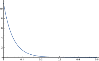
(a) $\mu=20$. Graph of $|\gamma_{k}(t)|$ for $k=(0,1,0)$ and for $t\in[0,0.5)$.

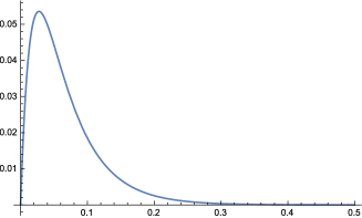
(b) $\mu=20$. Graph of $|\beta_{k}(t)|$ for $k=(0,1,0)$ and for $t\in[0,0.5)$.

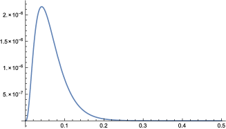
(c) $\mu=20$. Graph of $|\gamma_{k}(t)|$ for $k=(1,1,0)$ and for $t\in[0,0.5)$.

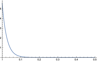
(d) $\mu=20$. Graph of $|\beta_{k}(t)|$ for $k=(1,1,0)$ and for $t\in[0,0.5)$.

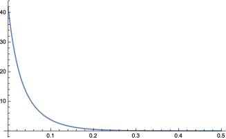
(e) $\mu=20$. Graph of $\mathcal{D}_{3}(t)$ for $t\in[0,0.5)$.

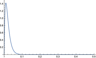
(f) $\mu=20$. Graph of $\epsilon_{3}(t)$ for $t\in[0,0.5)$.

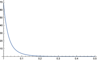
(g) $\mu=20$. Graph of $\mathcal{D}_{5}(t)$ for $t\in[0,0.5)$.

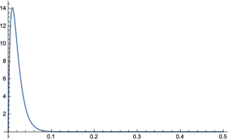
(h) $\mu=20$. Graph of $\epsilon_{5}(t)$ for $t\in[0,0.5)$.

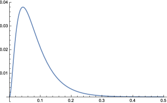
(i) $\mu=20$. Graph of ${\mathcal{R}}_{3}(t)$ for $t\in[0,0.5)$.

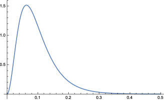
(j) $\mu=20$. Graph of ${\mathcal{R}}_{5}(t)$ for $t\in[0,0.5)$.

Figure 1: Plots related to the case $\mu=20$.

In the subsequent applications of the scheme (i)(ii)(iii) for several values of $\mu$, the graph of ${\mathcal{R}}_{5}$ is reported only in a case with rather large $\mu$, in which ${\mathcal{R}}_{5}(t)$ is small with respect to $\mathcal{D}_{5}(t)=\|\mathbf{u}_{G}(t)\|_{5}$; this fact makes the bound (7.20) interesting. In the other cases considered, ${\mathcal{R}}_{5}(t)$ is sensibly larger than $\mathcal{D}_{5}(t)$; this makes the bound (7.20) less interesting, so the graph of ${\mathcal{R}}_{5}$ is not so useful. Let us pass to exemplify the procedure (i)(ii)(iii) for some values of $\mu$. Case $\mu=20$. System (6.24) for the unknowns $\gamma_{k},\beta_{k}$ ($k\in G$) has been integrated on a time interval of length $T_{F}=0.5$. Figures 1(a)-1(d) report, as examples, the graphs of $|\gamma_{k}(t)|$, $|\beta_{k}(t)|$ for $k=(0,1,0)$ and $k=(1,1,0)$ (where $|z|:=\sqrt{\sum_{i=1}^{3}|z_{i}|^{2}}$ is the standard ${\mathbb{C}}^{3}$ norm). Figures 1(e)-1(h) report the graphs of the estimators $\mathcal{D}_{p},\epsilon_{p}$ for $p=3,5$ (the graphs of $\mathcal{D}_{p}$ for $p=4,6$ are omitted just for brevity).

The solution $\mathcal{R}_{3}$ of the control Cauchy problem (7.13) (7.14) is found to exist on the whole interval $[0,T_{F})=[0,0.5)$; its graph is given by Figure 1(i).

It turns out that condition (7.16) $(\mathcal{D}_{3}+{\mathcal{R}}_{3})(t_{1})\leqslant{\mu/{\hat{G}}_{3}}$ is fulfilled for any $t_{1}\in[0.01,0.5)$; this ensures that the solution of the MHD Cauchy problem (3.24) is global ($T=+\infty$) and decays exponentially as indicated by (7.17). For example, let us write down the estimate (7.17) choosing $t_{1}=0.25$; with appropriate roundings we have $(\mathcal{D}_{3}+{\mathcal{R}}_{3})(0.25)=0.186$ and ${\hat{G}}_{3}(\mathcal{D}_{3}+{\mathcal{R}}_{3})(0.25)=0.115$, so the cited equation gives

$$\|\mathbf{u}(t)\|_{3}\leqslant{0.186e^{-20(t-0.25)}\over 1-0.115\,e_{20}(t-0.25)}~{}\mbox{for $t\in[0.25,+\infty)$}~{}.$$ (7.21)

($e_{20}$ as in (5.9)). Figure 1(j) gives the graph of ${\mathcal{R}}_{5}(t)$ for $t\in[0,0.5)$. Of course, we have

$$\|\mathbf{u}(t)-\mathbf{u}_{G}(t)\|_{3}\leqslant{\mathcal{R}}_{3}(t),~{}\|\mathbf{u}(t)-\mathbf{u}_{G}(t)\|_{5}\leqslant{\mathcal{R}}_{5}(t)\quad\mbox{for $t\in[0,0.5)$}.$$ (7.22)

The first of these estimates is certainly interesting on the whole interval $[0,0.5)$, where ${\mathcal{R}}_{3}(t)$ is always much smaller than $\mathcal{D}_{3}(t):=\|\mathbf{u}_{G}(t)\|_{3}$ (${\mathcal{R}}_{3}(t)<\mathcal{D}_{3}(t)/100$ for $t\in[0,0.5)$). Concerning the second estimate, it should be pointed out that ${\mathcal{R}}_{5}(t)$ is smaller than $\mathcal{D}_{5}(t):=\|\mathbf{u}_{G}(t)\|_{5}$ on the whole interval $[0,0.5)$, and sensibly smaller on a shorter interval (${\mathcal{R}}_{5}(t)<\mathcal{D}_{5}(t)/2$ for $t\in[0,0.5)$ and ${\mathcal{R}}_{5}(t)<\mathcal{D}_{5}(t)/10$ for $t\in[0,0.047)$). Case $\mu=6$. System (6.24) for $\gamma_{k},\beta_{k}$ ($k\in G$) has been integrated on a time interval of length $T_{F}=2$. Figures 2(a)-2(d) give the graphs of $|\gamma_{k}(t)|$, $|\beta_{k}(t)|$ for $k=(0,1,0)$ and $k=(1,1,0)$. Figures 2(e)-2(f) report the graphs of the estimators $\mathcal{D}_{3}$, $\epsilon_{3}$.

The solution $\mathcal{R}_{3}(t)$ of the control Cauchy problem (7.13) (7.14) is found to exist on the whole interval $[0,T_{F})=[0,2)$; its graph is given by Figure 2(g). Condition (7.16) $(\mathcal{D}_{3}+{\mathcal{R}}_{3})(t_{1})\leqslant{\mu/{\hat{G}}_{3}}$ is fulfilled for all $t_{1}\in[0.32,2)$; this ensures that the solution $\mathbf{u}$ of the MHD Cauchy problem (3.24) is global ($T=+\infty$) and decays exponentially as indicated by (7.17). For example, let us write down the estimate (7.17) choosing $t_{1}=1$; with appropriate roundings we have $(\mathcal{D}_{3}+{\mathcal{R}}_{3})(1)=1.09$ and ${\hat{G}}_{3}(\mathcal{D}_{3}+{\mathcal{R}}_{3})(1)=0.68$, so the cited equation gives

$$\|\mathbf{u}(t)\|_{3}\leqslant{1.09e^{-6(t-1)}\over 1-0.68\,e_{6}(t-1)}~{}\mbox{for $t\in[1,+\infty)$}~{}.$$ (7.23)

($e_{6}$ as in (5.9)). We have

$$\|\mathbf{u}(t)-\mathbf{u}_{G}(t)\|_{3}\leqslant{\mathcal{R}}_{3}(t)\quad\mbox{for $t\in[0,2)$}.$$ (7.24)

This estimate is especially interesting when ${\mathcal{R}}_{3}(t)$ is sensibly smaller than $\mathcal{D}_{3}(t):=\|\mathbf{u}_{G}(t)\|_{3}$. This does not hold on the whole interval $[0,2)$, but it is true on shorter intervals: for example, ${\mathcal{R}}_{3}(t)<\mathcal{D}_{3}(t)/10$ for $t\in[0,0.11]$. Case $\mu=5$. System (6.24) for $\gamma_{k},\beta_{k}$ ($k\in G$) has been integrated on a time interval of length $T_{F}=2$. Figures 3(a)-3(d) give the graphs of $|\gamma_{k}(t)|$, $|\beta_{k}(t)|$ for $k=(0,1,0)$ and $k=(1,1,0)$. Figures 3(e)-3(f) report the graphs of the estimators $\mathcal{D}_{3}$, $\epsilon_{3}$.

The solution $\mathcal{R}_{3}$ of the control Cauchy problem (7.13) (7.14) has domain $[0,T_{\tt{c}})$ where $T_{\tt{c}}=0.3238...$; $\mathcal{R}_{3}(t)$ is found to diverge for $t\to T_{\tt{c}}$. Figure 3(g) contains the graph of $\mathcal{R}_{3}$.

Due to the features of our general scheme, the solution $\mathbf{u}$ of the MHD Cauchy problem (3.24) is granted to exist (at least) up to time $T_{\tt{c}}$. We have

$$\|\mathbf{u}(t)-\mathbf{u}_{G}(t)\|_{3}\leqslant{\mathcal{R}}_{3}(t)\quad\mbox{for $t\in[0,T_{\tt{c}})=[0,0.3238...)$};$$ (7.25)

this inequality is especially interesting in the smaller interval $[0,0.1]$, where ${\mathcal{R}}_{3}(t)$ is sensibly smaller than $\mathcal{D}_{3}(t):=\|\mathbf{u}_{G}(t)\|_{3}$ (${\mathcal{R}}_{3}(t)<\mathcal{D}_{3}(t)/10$ for $t\in[0,0.1]$). Case $\mu=0$. Again, system (6.24) for $\gamma_{k},\beta_{k}$ ($k\in G$) has been integrated on a time interval of length $T_{F}=2$. Figures 4(a)-4(d) give the graphs of $|\gamma_{k}(t)|$, $|\beta_{k}(t)|$ for $k=(0,1,0)$ and $k=(1,1,0)$. Figures 4(e)-4(f) report the graphs of the estimators $\mathcal{D}_{3}$, $\epsilon_{3}$.

The solution $\mathcal{R}_{3}$ of the control Cauchy problem (7.13) (7.14) has domain $[0,T_{\tt{c}})$ where $T_{\tt{c}}=0.1211...$, and diverges for $t\to T_{\tt{c}}$. The graph of $\mathcal{R}_{3}$ is presented in Figure 4(g).

The solution $\mathbf{u}$ of the MHD Cauchy problem (3.24) is granted to exist up to time $T_{\tt{c}}$. We have

$$\|\mathbf{u}(t)-\mathbf{u}_{G}(t)\|_{3}\leqslant{\mathcal{R}}_{3}(t)\quad\mbox{for $t\in[0,T_{\tt{c}})=[0,0.1211...)$};$$ (7.26)

this inequality is especially interesting in the smaller interval $t\in[0,0.067]$, where ${\mathcal{R}}_{3}(t)$ is sensibly smaller than $\mathcal{D}_{3}(t):=\|\mathbf{u}_{G}(t)\|_{3}$ (${\mathcal{R}}_{3}(t)<\mathcal{D}_{3}(t)/10$ for $t\in[0,0.067]$) Other cases. We have performed computations similar to those described before even for $\mu=10$ and $\mu=3$. As in the cases $\mu=20$ and $\mu=6$, for $\mu=10$ we can grant global existence for the exact solution $\mathbf{u}$ of the MHD Cauchy problem (3.24). As in the cases $\mu=5$ and $\mu=0$, for $\mu=3$ we can grant existence of the solution $\mathbf{u}$ only on a finite interval; in fact the solution $\mathcal{R}_{3}(t)$ of the control Cauchy problem (7.13) (7.14) diverges for $t\to T_{\tt{c}}=0.1853...$, so we can ensure existence of $\mathbf{u}$ only up to $T_{\tt{c}}$.

Acknowledgments L.P. acknowledges support from: INdAM, Gruppo Nazionale per la Fisica Matematica; Istituto Nazionale di Fisica Nucleare; MIUR, PRIN 2010 Research Project “Geometric and analytic theory of Hamiltonian systems in finite and infinite dimensions”; Università degli Studi di Milano.

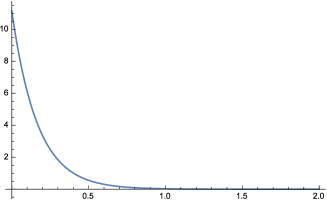
(a) $\mu=6$. Graph of $|\gamma_{k}(t)|$ for $k=(0,1,0)$ and for $t\in[0,2)$.

(b) $\mu=6$. Graph of $|\beta_{k}(t)|$ for $k=(0,1,0)$ and for $t\in[0,2)$.

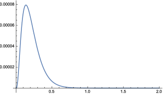
(c) $\mu=6$. Graph of $|\gamma_{k}(t)|$ for $k=(1,1,0)$ and for $t\in[0,2)$.

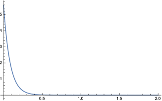
(d) $\mu=6$. Graph of $|\beta_{k}(t)|$ for $k=(1,1,0)$ and for $t\in[0,2)$.

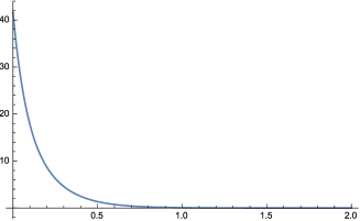
(e) $\mu=6$. Graph of $\mathcal{D}_{3}(t)$ for $t\in[0,2)$.

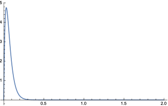
(f) $\mu=6$. Graph of $\epsilon_{3}(t)$ for $t\in[0,2)$.

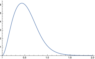
(g) $\mu=6$. Graph of ${\mathcal{R}}_{3}(t)$.

Figure 2: Plots related to the case $\mu=6$.

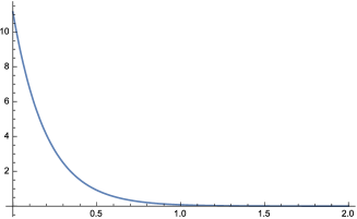
(a) $\mu=5$. Graph of $|\gamma_{k}(t)|$ for $k=(0,1,0)$ and for $t\in[0,2)$.

(b) $\mu=5$. Graph of $|\beta_{k}(t)|$ for $k=(0,1,0)$ and for $t\in[0,2)$.

(c) $\mu=5$. Graph of $|\gamma_{k}(t)|$ for $k=(1,1,0)$ and for $t\in[0,2)$.

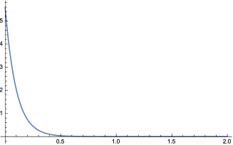
(d) $\mu=5$. Graph of $|\beta_{k}(t)|$ for $k=(1,1,0)$ and for $t\in[0,2)$.

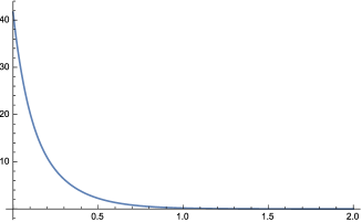
(e) $\mu=5$. Graph of $\mathcal{D}_{3}(t)$ for $t\in[0,2)$.

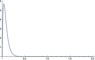
(f) $\mu=5$. Graph of $\epsilon_{3}(t)$ for $t\in[0,2)$.

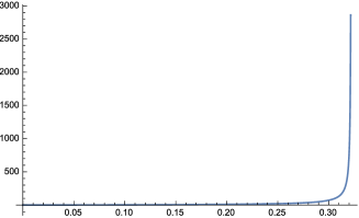
(g) $\mu=5$. Graph of ${\mathcal{R}}_{3}(t)$. This function diverges as $t\rightarrow T_{c}$ with $T_{c}=0.3238...$.

Figure 3: Plots related to the case $\mu=5$.

(a) $\mu=0$. Graph of $|\gamma_{k}(t)|$ for $k=(0,1,0)$ and for $t\in[0,2)$.

(b) $\mu=0$. Graph of $|\beta_{k}(t)|$ for $k=(0,1,0)$ and for $t\in[0,2)$.

(c) $\mu=0$. Graph of $|\gamma_{k}(t)|$ for $k=(1,1,0)$ and for $t\in[0,2)$.

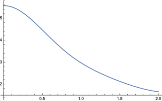
(d) $\mu=0$. Graph of $|\beta_{k}(t)|$ for $k=(1,1,0)$ and for $t\in[0,2)$.

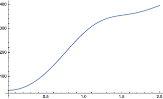
(e) $\mu=0$. Graph of $\mathcal{D}_{3}(t)$ for $t\in[0,2)$.

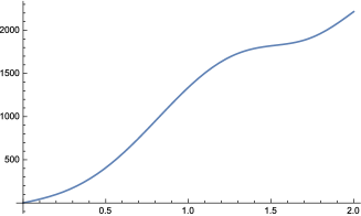
(f) $\mu=0$. Graph of $\epsilon_{3}(t)$ for $t\in[0,2)$.

(g) $\mu=0$. Graph of ${\mathcal{R}}_{3}(t)$. This function diverges as $t\rightarrow T_{c}$ with $T_{c}=0.1211...$.

Figure 4: Plots related to the case $\mu=0$.

Appendix A Appendix. Proof of Eqs. (3.17)- (3.20)

In this appendix we frequently use the following inequalities, holding for all $\alpha,\beta,\gamma,\delta$ $\in{\mathbb{R}}$:

$$\alpha\gamma+\beta\delta\leqslant\sqrt{\alpha^{2}+\beta^{2}}\sqrt{\gamma^{2}+\delta^{2}}~{},$$ (A.1)

$$\gamma+\delta\leqslant\sqrt{2}\sqrt{\gamma^{2}+\delta^{2}}~{}.$$ (A.2)

Eq. (A.1) is just the Schwartz inequality for the standard inner product of ${\mathbb{R}}^{2}$; Eq. (A.2) is the specialization of (A.1) to the case $\alpha=\beta=1$. We will also use the parallelogram law

$$\|x+y\|^{2}+\|x-y\|^{2}=2\|x\|^{2}+2\|y\|^{2}~{},$$ (A.3)

holding for all elements $x,y$ of any Hilbert space with norm $\|~{}\|$.

A.1

Proposition. Consider two reals $p\geqslant n>d/2$. For $\mathbf{v}\in\mathbf{H}^{{p}}_{\Sigma 0}$, $\mathbf{w}\in\mathbf{H}^{{p+1}}_{\Sigma 0}$ one has the inequality

$$\lVert{\mbox{\boldmath$\mathscr{P}$}}(\mathbf{v},\mathbf{w})\rVert_{{p}}\,\,\leqslant\frac{1}{2}(\sqrt{2}K_{pn})(\lVert\mathbf{v}\rVert_{{p}}\lVert\mathbf{w}\rVert_{{{n}+1}}+\lVert\mathbf{v}\rVert_{{n}}\lVert\mathbf{w}\rVert_{{p+1}}),$$ (A.4)

where $K_{pn}$ is a constant fulfilling Eq. (2.20). Thus, Eqs. (3.17) (3.19) hold.

Proof. Let us fix $p\geqslant n>d/2$ and $\mathbf{v}=(v,b)\in\mathbf{H}^{{p}}_{\Sigma 0}$, $\mathbf{w}=(w,c)\in\mathbf{H}^{{p+1}}_{\Sigma 0}$. The definition (3.8) of $\mathscr{P}$ gives

$$\lVert{\mbox{\boldmath$\mathscr{P}$}}(\mathbf{v},\mathbf{w})\rVert_{{p}}=\sqrt{\lVert{\mathscr{P}}(v,w)-{\mathscr{P}}(b,c)\rVert_{{p}}^{2}+\lVert{\mathscr{P}}(v,c)-{\mathscr{P}}(b,w)\rVert_{{p}}^{2}}~{}.$$ (A.5)

Let us note that

$$\lVert{\mathscr{P}}(v,w)-{\mathscr{P}}(b,c)\rVert_{{p}}\leqslant\lVert{\mathscr{P}}(v,w)\rVert_{{p}}+\lVert{\mathscr{P}}(b,c)\rVert_{{p}}$$

$$\leqslant\frac{1}{2}K_{pn}(\lVert v\rVert_{{p}}\lVert w\rVert_{n+1}+\lVert v\rVert_{n}\lVert w\rVert_{{p+1}}+\lVert b\rVert_{{p}}\lVert c\rVert_{n+1}+\lVert b\rVert_{n}\lVert c\rVert_{{p+1}})$$

$$\leqslant\frac{1}{2}K_{pn}(\sqrt{\lVert v\rVert_{{p}}^{2}+\lVert b\rVert_{{p}}^{2}}\sqrt{\lVert w\rVert_{n+1}^{2}+\lVert c\rVert_{n+1}^{2}}+\sqrt{\lVert v\rVert_{n}^{2}+\lVert b\rVert_{n}^{2}}\sqrt{\lVert w\rVert_{{p+1}}^{2}+\lVert c\rVert_{{p+1}}^{2}}\,)$$

$$=\frac{1}{2}K_{pn}(\lVert\mathbf{v}\rVert_{{p}}\lVert\mathbf{w}\rVert_{n+1}+\lVert\mathbf{v}\rVert_{n}\lVert\mathbf{w}\rVert_{{p+1}}).$$ (A.6)

In the above chain of relations, to go from the first to the second line we have used the inequality (2.20); to go from the second to the third line, after exchanging the order of summands we have used twice Eq. (A.1).

Similarly, we obtain

$$\lVert{\mathscr{P}}(v,c)-{\mathscr{P}}(b,w)\rVert_{{p}}\leqslant\frac{1}{2}K_{pn}(\lVert\mathbf{v}\rVert_{{p}}\lVert\mathbf{w}\rVert_{n+1}+\lVert\mathbf{v}\rVert_{n}\lVert\mathbf{w}\rVert_{{p+1}}).$$ (A.7)

Consequently, from (A.6) and (A.7), we obtain

$$\lVert{\mbox{\boldmath$\mathscr{P}$}}(\mathbf{v},\mathbf{w})\rVert_{{p}}=\sqrt{\lVert{\mathscr{P}}(v,w)-{\mathscr{P}}(b,c)\rVert_{{p}}^{2}+\lVert{\mathscr{P}}(v,c)-{\mathscr{P}}(b,w)\rVert_{{p}}^{2}}$$

$$\leqslant\sqrt{\frac{K_{pn}^{2}}{4}(\lVert\mathbf{v}\rVert_{{p}}\lVert\mathbf{w}\rVert_{n+1}+\lVert\mathbf{v}\rVert_{n}\lVert\mathbf{w}\rVert_{{p+1}})^{2}+\frac{K_{pn}^{2}}{4}(\lVert\mathbf{v}\rVert_{{p}}\lVert\mathbf{w}\rVert_{n+1}+\lVert\mathbf{v}\rVert_{n}\lVert\mathbf{w}\rVert_{{p+1}})^{2}}$$

$$=\frac{K_{pn}}{\sqrt{2}}(\lVert\mathbf{v}\rVert_{{p}}\lVert\mathbf{w}\rVert_{n+1}+\lVert\mathbf{v}\rVert_{n}\lVert\mathbf{w}\rVert_{{p+1}}),$$

which yields the inequality (A.4). $\square$

A.2

Proposition. Consider two reals $p\geqslant n>d/2+1$. For $\mathbf{v}\in\mathbf{H}^{{p}}_{\Sigma 0}$, $\mathbf{w}\in\mathbf{H}^{{p+1}}_{\Sigma 0}$ one has the inequality

$$|\langle{\mbox{\boldmath$\mathscr{P}$}}(\mathbf{v},\mathbf{w})|\mathbf{w}\rangle_{{p}}|\leqslant\frac{1}{2}(\sqrt{2}G_{pn})(\lVert\mathbf{v}\rVert_{{p}}\lVert\mathbf{w}\rVert_{{n}}+\lVert\mathbf{v}\rVert_{{n}}\lVert\mathbf{w}\rVert_{{p}})\lVert\mathbf{w}\rVert_{{p}},$$ (A.8)

where $G_{pn}$ is a constant fulfilling (2.21). Thus, Eqs. (3.18) (3.20) hold.

Proof. In the sequel $p\geqslant n>d/2+1$ and $\mathbf{v}=(v,b)\in\mathbf{H}^{{p}}_{\Sigma 0}$, $\mathbf{w}=(w,c)\in\mathbf{H}^{{p+1}}_{\Sigma 0}$ are fixed; we proceed in several steps.

Step 1. One has

$$\langle{\mbox{\boldmath$\mathscr{P}$}}(\mathbf{v},\mathbf{w})|\mathbf{w}\rangle_{p}=\langle{\mathscr{P}}(v,w)|w\rangle_{p}+\langle{\mathscr{P}}(v,c)|c\rangle_{p}+$$ (A.9)

$$-\frac{1}{2}\langle{\mathscr{P}}(b,w+c)|w+c\rangle_{p}+\frac{1}{2}\langle{\mathscr{P}}(b,w-c)|w-c\rangle_{p}~{}.$$

To prove this, we note that Eq. (3.8) for $\mathscr{P}$ implies

$$\begin{split}\langle{\mbox{\boldmath$\mathscr{P}$}}(\mathbf{v},\mathbf{w})|\mathbf{w}\rangle_{p}=\langle({\mathscr{P}}(v,w)-{\mathscr{P}}(b,c),{\mathscr{P}}(v,c)-{\mathscr{P}}(b,w))|(w,c)\rangle_{p}\\ =\langle{\mathscr{P}}(v,w)|w\rangle_{p}-\langle{\mathscr{P}}(b,c)|w\rangle_{p}+\langle{\mathscr{P}}(v,c)|c\rangle_{p}-\langle{\mathscr{P}}(b,w)|c\rangle_{p}~{}.\end{split}$$ (A.10)

On the other hand, by elementary manipulations relying on the bilinearity of ${\mathscr{P}}$ and $\langle~{}|~{}\rangle_{p}$ we get

$$\langle{\mathscr{P}}(b,c)|w\rangle_{p}+\langle{\mathscr{P}}(b,w)|c\rangle_{p}=\frac{1}{2}\langle{\mathscr{P}}(b,w+c)|w+c\rangle_{p}-\frac{1}{2}\langle{\mathscr{P}}(b,w-c)|w-c\rangle_{p}$$ (A.11)

and inserting this result into (A.10) we get the thesis (A.9).

Step 2. One has

$$|\langle{\mbox{\boldmath$\mathscr{P}$}}(\mathbf{v},\mathbf{w})|\mathbf{w}\rangle_{p}|\leqslant|\langle{\mathscr{P}}(v,w)|w\rangle_{p}|+|\langle{\mathscr{P}}(v,c)|c\rangle_{p}|+$$ (A.12)

$$+\frac{1}{2}|\langle{\mathscr{P}}(b,w+c)|w+c\rangle_{p}|+\frac{1}{2}|\langle{\mathscr{P}}(b,w-c)|w-c\rangle_{p}|~{}.$$

This is an obvious consequence of (A.9).

Step 3. One has

$$|\langle{\mathscr{P}}(v,w)|w\rangle_{p}|+|\langle{\mathscr{P}}(v,c)|c\rangle_{p}|\leqslant\frac{1}{2}G_{pn}\|v\|_{p}\|\mathbf{w}\|_{n}\|\mathbf{w}\|_{p}+\frac{1}{2}G_{pn}\|v\|_{n}\|\mathbf{w}\|^{2}_{p}~{}.$$ (A.13)

In fact, due to (2.21),

$$|\langle{\mathscr{P}}(v,w)|w\rangle_{p}|\leqslant\frac{1}{2}G_{pn}(\|v\|_{p}\|w\|_{n}+\|v\|_{n}\|w\|_{p})\|w\|_{p}$$ (A.14)

$$=\frac{1}{2}G_{pn}(\|v\|_{p}\|w\|_{n}\|w\|_{p}+\|v\|_{n}\|w\|^{2}_{p})~{};$$

one treats similarly the term $|\langle{\mathscr{P}}(v,c)|c\rangle_{p}|$, so

$$|\langle{\mathscr{P}}(v,w)|w\rangle_{p}|+|\langle{\mathscr{P}}(v,c)|c\rangle_{p}|$$ (A.15)

$$\leqslant\frac{1}{2}G_{pn}(\|v\|_{p}\|w\|_{n}\|w\|_{p}+\|v\|_{n}\|w\|^{2}_{p})+\frac{1}{2}G_{pn}(\|v\|_{p}\|c\|_{n}\|c\|_{p}+\|v\|_{n}\|c\|^{2}_{p})$$

$$=\frac{1}{2}G_{pn}\|v\|_{p}(\|w\|_{n}\|w\|_{p}+\|c\|_{n}\|c\|_{p})+\frac{1}{2}G_{pn}\|v\|_{n}(\|w\|^{2}_{p}+\|c\|^{2}_{p})~{}.$$

On the other hand, due to (A.1)

$$\|w\|_{n}\|w\|_{p}+\|c\|_{n}\|c\|_{p}\leqslant\sqrt{\|w\|^{2}_{n}+\|c\|^{2}_{n}}\sqrt{\|w\|^{2}_{p}+\|c\|^{2}_{p}}=\|\mathbf{w}\|_{n}\|\mathbf{w}\|_{p}~{},$$ (A.16)

while

$$\|w\|^{2}_{p}+\|c\|^{2}_{p}=\|\mathbf{w}\|^{2}_{p}~{};$$ (A.17)

inserting Eqs. (A.16) (A.17) into (A.14) we get the thesis (A.13).

Step 4. One has

$$\frac{1}{2}|\langle{\mathscr{P}}(b,w+c)|w+c\rangle_{p}|+\frac{1}{2}|\langle{\mathscr{P}}(b,w-c)|w-c\rangle_{p}|$$ (A.18)

$$\leqslant\frac{1}{2}G_{pn}\|b\|_{p}\|\mathbf{w}\|_{n}\|\mathbf{w}\|_{p}+\frac{1}{2}G_{pn}\|b\|_{n}\|\mathbf{w}\|^{2}_{p}~{}.$$

In fact, using the inequality (2.21) for each one of the above two terms we get

$$\frac{1}{2}|\langle{\mathscr{P}}(b,w+c)|w+c\rangle_{p}|+\frac{1}{2}|\langle{\mathscr{P}}(b,w-c)|w-c\rangle_{p}|$$ (A.19)

$$\leqslant\frac{1}{4}G_{pn}(\|b\|_{p}\|w+c\|_{n}+\|b\|_{n}\|w+c\|_{p})\|w+c\|_{p}+\frac{1}{4}G_{pn}(\|b\|_{p}\|w-c\|_{n}+\|b\|_{n}\|w-c\|_{p})\|w-c\|_{p}$$

$$=\frac{1}{4}G_{pn}\|b\|_{p}(\|w+c\|_{n}\|w+c\|_{p}+\|w-c\|_{n}\|w-c\|_{p})+\frac{1}{4}G_{pn}\|b\|_{n}(\|w+c\|^{2}_{p}+\|w-c\|^{2}_{p})~{};$$

from here and from Eq. (A.1) we infer

$$\frac{1}{2}|\langle{\mathscr{P}}(b,w+c)|w+c\rangle_{p}|+\frac{1}{2}|\langle{\mathscr{P}}(b,w-c)|w-c\rangle_{p}|$$ (A.20)

$$\leqslant\frac{1}{4}G_{pn}\|b\|_{p}\sqrt{\|w+c\|^{2}_{n}+\|w-c\|^{2}_{n}}\sqrt{\|w+c\|^{2}_{p}+\|w-c\|^{2}_{p}}+\frac{1}{4}G_{pn}\|b\|_{n}(\|w+c\|^{2}_{p}+\|w-c\|^{2}_{p})~{}.$$

On the other hand, the parallelogram law (A.3) for the Hilbert spaces $\mathbb{H}^{{n}}_{\Sigma 0},\mathbb{H}^{{p}}_{\Sigma 0}$ gives

$$\|w+c\|^{2}_{n}+\|w-c\|^{2}_{n}=2\|w\|^{2}_{n}+2\|c\|^{2}_{n}=2\|\mathbf{w}\|^{2}_{n}~{},$$ (A.21)

$$\|w+c\|^{2}_{p}+\|w-c\|^{2}_{p}=2\|w\|^{2}_{p}+2\|c\|^{2}_{p}=2\|\mathbf{w}\|^{2}_{p}$$

and inserting Eq. (A.21) into (A.20) we get the thesis (A.18).

Step 5. The inequality (A.8) holds (so the proof is concluded). In fact, from Eqs. (A.12) (A.13) (A.18) we get:

$$|\langle{\mbox{\boldmath$\mathscr{P}$}}(\mathbf{v},\mathbf{w})|\mathbf{w}\rangle_{p}|$$ (A.22)

$$\leqslant\frac{1}{2}G_{pn}(\|v\|_{p}+\|b\|_{p})\|\mathbf{w}\|_{n}\|\mathbf{w}\|_{p}+\frac{1}{2}G_{pn}(\|v\|_{n}+\|b\|_{n})\|\mathbf{w}\|^{2}_{p}~{}.$$

On the other hand, Eq. (A.2) gives

$$\|v\|_{p}+\|b\|_{p}\leqslant\sqrt{2}\sqrt{\|v\|^{2}_{p}+\|b\|^{2}_{p}}=\sqrt{2}\,\|\mathbf{v}\|_{p}~{},$$ (A.23)

$$\|v\|_{n}+\|b\|_{n}\leqslant\sqrt{2}\sqrt{\|v\|^{2}_{n}+\|b\|^{2}_{n}}=\sqrt{2}\,\|\mathbf{v}\|_{n}~{},$$

and inserting these inequalities into (A.22) we obtain the thesis (A.8). $\square$

References

- [1] S.I. Chernyshenko, P. Constantin, J.C. Robinson, E.S. Titi, A posteriori regularity of the three-dimensional Navier-Stokes equations from numerical computations, J. Math. Phys. 48 (2007), 065204/1-10.
- [2] M. Dashti, J.C. Robinson, An a posteriori condition on the numerical approximation of the Navier-Stokes equations for the existence of a strong solution, SIAM J. Numer. Anal. 46 (2008), 3136-3150.
- [3] J.C. Robinson, W. Sadowski, Numerical verification of regularity in the three-dimensional Navier-Stokes equations for bounded sets of initial data, Asymptot. Anal. 59 (2008), 39-50.
- [4] C. Morosi and L. Pizzocchero, On approximate solutions of the incompressible Euler and Navier-Stokes equations, Nonlinear Analysis, 75 (2012), 2209-2235.
- [5] C. Morosi, M. Pernici, L. Pizzocchero, Large order Reynolds expansions for the Navier-Stokes equations, Appl. Math. Letters 49 (2015), 58-66.
- [6] C. Morosi, M. Pernici, L. Pizzocchero, A posteriori estimates for Euler and Navier-Stokes equations, in “Hyperbolic Problems: Theory, Numerics and Applications. Proceedings of the XIV International Conference held in Padova (June 25-29, 2012)”, edited by F. Ancona, A. Bressan, P. Marcati, A. Marson, AIMS Series on Applied Mathematics 8 (2014), 847-855.
- [7] C. Morosi, L. Pizzocchero, Smooth solutions of the Euler and Navier-Stokes equations from the a posteriori analysis of approximate solutions, Nonlinear Analysis, 113 (2015), 298-308.
- [8] D. Blömker, C. Nolde, J. Robinson, Rigorous Numerical Verification of Uniqueness and Smoothness in a Surface Growth Model, Journal of Mathematical Analysis and Applications 429(1) (2015), 311-325.
- [9] D. Blömker, M. Romito, Stochastic PDEs and lack of regularity. (A surface growth equation with noise: existence, uniqueness, and blow-up), Jahresbericht der Deutschen Mathematiker-Vereinigung, 117(4) (2015), 233-286.
- [10] C. Nolde, “Global Regularity and Uniqueness of Solutions in a Surface Growth Model Using Rigorous A-Posteriori Methods”, ISBN: 978-3-8325-4453-9, Logos Verlag Berlin (2017).
- [11] D. Blömker, M. Kamrani, Numerically Computable A Posteriori-Bounds for SPDEs, arXiv:1702.01347v3 [math.NA] 13 Nov 2017, to appear in BIT Numerical Mathematics
- [12] C. Morosi and L. Pizzocchero, On the constants in a Kato inequality for the Euler and Navier-Stokes equations, Comm. on Pure and Applied Analysis, 11 (2012), 557-586.
- [13] C. Morosi and L. Pizzocchero, On the constants in a basic inequality for the Euler and Navier-Stokes equations, Applied Mathematics Letters 26 (2013), 277-284.
- [14] C. Morosi, M. Pernici, L. Pizzocchero, New results on the constants in some inequalities for the Navier-Stokes quadratic nonlinearity, Applied Mathematics and Computation, 308 (2017), 54-72.
- [15] P. D. Mininni, A. G. Pouquet and D. C. Montgomery, Small-scale structures in three-dimensional magnetohydrodynamic turbulence, Phys. Rev. Lett., 97 (2006), 244503/1-4.
- [16] C. Cartes, M.D. Bustamante, A. Pouquet and M.E. Brachet, Capturing reconnection phenomena using generalized Eulerian-Lagrangian description in Navier-Stokes and resistive MHD, Fluid Dyn. Res., 41 (2009), 011404/1-14.
- [17] T. Kato, Nonstationary flows of viscous and ideal fluids in , J. Funct. Anal., 9 (1972), 296-305.
- [18] P. Constantin, C. Foias, “Navier Stokes equations”, Chicago University Press (1988).
- [19] R. Temam, Local existence of solutions of the Euler equation of incompressible perfect fluids, in “Turbulence and Navier Stokes equation”, Proceedings of the Orsay Conference, Lecture Notes in Mathematics 565 (1976), 184-193.
- [20] J.T. Beale, T. Kato, A.J. Majda, Remarks on the breakdown of smooth solutions for the 3D Euler equations, Commun. Math. Phys. 94 (1984), 61-66.
- [21] J. C. Robinson, W. Sadowski, R. P. Silva, Lower bounds on blow up solutions of the three-dimensional Navier-Stokes equations in homogeneous Sobolev spaces, J. Math. Phys. 53 (2012), 115618, 15pp.
- [22] G. Duvaut, J. L. Lions, Inéquations en thermoélasticité et magnétohydrodynamique, Arch. Rational Mech. Anal. 46 (1972), 241-279.
- [23] M. Sermange and R. Temam, Some mathematical questions related to the MHD equations, Comm. on Pure and Applied Mathematics, 36 (1983), 635-664.
- [24] P. G. Schmidt, On a magnetohydrodynamic problem of Euler type, Journal of Diff. Equations, 74 (1988), 318-335.
- [25] R. E. Caflisch, I. Klapper, G. Steele, Remarks on Singularities, Dimension and Energy Dissipation for Ideal Hydrodynamics and MHD, Commun. Math. Phys. 184 (1997), 443-455.
- [26] J. Fan, T. Ozawa, Regularity criteria for the magnetohydrodynamic equations with partial viscous terms and the Leray-- MHD model, Kinetic Related Models 2(2) (2009), 293-305.
- [27] C. L. Fefferman, D. S. McCormick, J. C. Robinson, J.L. Rodrigo, Higher order commutator estimates and local existence for the non-resistive MHD equations and related models, Journal of Functional Analysis 267 (2014), 1035-1056.
- [28] C. L. Fefferman, D. S. McCormick, J. C. Robinson, J.L. Rodrigo, Local Existence for the Non-Resistive MHD Equations in Nearly Optimal Sobolev Spaces, Arch. Rational Mech. Anal. 223 (2017), 677-691.
- [29] T. Petry, On the stability of the Abramov transfer for differential algebraic equations of index 1, SIAM J. Numer. Anal. 35 (1998), 201-216.
- [30] V. Lakshmikantham, S. Leela, “Differential and integral inequalities”, Volume I, Academic Press, New York (1969).
- [31] D.S. Mitrinovic, J.E. Pecaric, A.M. Fink, “Inequalities involving functions and their integrals and derivatives”, Kluwer, Dordrecht (1991).
- [32] S. M. Rump, INTLAB, http://www.ti3.tu-harburg.de/rump/intlab/.
- [33] Fredrik Johansson, Arb - a C library for arbitrary-precision ball arithmetic, http://arblib.org/.
- [34] S. M. Rump, Verification methods: rigorous results using floating point arithmetic, Acta Numerica 19 (2010), 287-449.