Effect of extended $\nu$ production region on collective oscillations in supernovae

Abstract

In supernovae neutrinos are emitted from a region with a width $r_{\rm eff}$ of a few kilometers (rather than from a surface of infinitesimal width). We study the effect of integration (averaging) over such an extended emission region on collective oscillations. The averaging leads to additional suppression of the correlation (off-diagonal element of the density matrix) by a factor $\sim 1/r_{\rm eff}V_{e}\sim 10^{-10}$, where $V_{e}$ is the matter potential. This factor enters the initial condition for further collective oscillations and, consequently, leads to a delay of the strong flavour transitions. We justify and quantify this picture using a simple example of collective effects in two intersecting fluxes. We have derived the evolution equation for the density matrix elements integrated over the emission region and solved it both numerically and analytically. For the analytic solution we have used linearized equations. We show that the delay of the development of the instability and the collective oscillations depends on the suppression factor due to the averaging (integration) logarithmically. If the instability develops inside the production region, the integration leads not only to a delay but also to a modification of the exponential grow.

1 Introduction

In most studies of the neutrino flavour conversion and, in particular, effects of collective oscillations, the emission of neutrinos is considered from a neutrino sphere – a surface of zero width, so that further neutrino evolution proceeds in the free streaming regime. The radius of the neutrino sphere $R_{\nu\rm sphere}$ is defined in terms of the optical depth $\tau(r)$ as [1]

$$\tau(R_{\nu\rm sphere})=\frac{2}{3},$$ (1.1)

where

$$\tau(r)\equiv\int_{r}^{\infty}\Gamma(r^{\prime})dr^{\prime},$$ (1.2)

and $\Gamma$ is the collision rate. Thus, $\tau$ is the probability of collision from the emission point $r$ to $\infty$, and according to (1.1) and (1.2), $R_{\nu\rm sphere}$ is the radius from which the probability for neutrinos to escape without collisions is 1/3.

This zero width approximation was justified by the fact that in the production region, the matter density is very large. Hence the in matter mixing angle is small and, consequently, any flavour evolution are strongly suppressed. Therefore, the flavour evolution was considered from some surface outside the production region [2].

In reality, the region of neutrino production $r_{\rm eff}$ is rather large (we quantify this in Section 2). In [3] it was shown that the zero width approximation may not be correct: in spite of the smallness of mixing, the integration over the neutrino production region leads to additional suppression of flavour transitions. According to [3], strong transitions can be interpreted as a parametric effect driven by periodic modulations of the background potentials. The bigger the amplitude of modulations, the faster the transition. Therefore any averaging, which diminishes the depth of modulations $d$, will suppress the transition. The spatial scale of strong transitions $L_{\rm par}$ is inversely proportional to the depth: $L_{\rm par}\propto 1/d$. Consequently, the averaging leads to an increase of $L_{\rm par}$, i.e., delay of the transition. Since the potential induced by neutrinos (which drives collective oscillations) decreases quickly, a delay may mean that the transition never occurs. Here the delay is linear in $V_{e}r_{\rm eff}$, where $V_{e}$ is the matter potential, since the instability develops linearly with distance.

The solvable example considered in [3] has one important shortcoming: $\nu\nu$ interactions in the background neutrino flux are neglected. With $\nu\nu$ interactions being included, parametric effects can be more complicated and the instability develops much faster.

In this paper, we will explore effects of averaging over the neutrino production region in the presence of $\nu\nu$ interactions in the background. Our approach is the following: We study the integration effect using a simple and symmetric model in which collective effects show up. Namely, the model with two intersecting beams with a single energy and equal numbers of neutrinos and antineutrinos. Then we argue that the results obtained in this model are generic and to some extent should be reproduced in more realistic models. We show that the integration (averaging) leads to the suppression of the initial flavour transition by a factor $1/V_{e}r_{\rm eff}$. This suppression in turn leads to a delay (in distance) of the development of the instability and strong collective effects. The delay is given by the logarithm of the suppression factor: $\log(1/V_{e}r_{\rm eff})$. If the instability starts in the production region, the averaging also modifies the exponential growth of the transition.

The paper is organised as follows. In Section 2 we make realistic estimations of the effective width of the production region $r_{\rm eff}$ and compute suppression of the conversion in the case of negligible collective oscillations in the production region which is justified in the very early phases of evolution. In Section 3 we consider the simplest system of two intersecting neutrino fluxes in which $\nu\nu$ interactions are included and study the effect of integration over the production region. In Section 4 using the linearised evolution equations, we give an analytic description of the conversion. The analytic results are in very good agreement with the results of numerical computations. In Section 5, using the analytic formulas, we extrapolate the results to parameters that are more realistic for the situation in supernovae. We conclude in Section 6. Some details of the computations are given in the appendices.

2 Effective emission width and suppression of the initial correlation

In this section we consider realistic conditions (density profiles) in supernovas, but neglect effects of $\nu\nu$ interactions, which is justified in the early phases of the flavour evolution (see Section 4). Indeed, at high densities close to the proto-neutron star, collective oscillations mainly manifest themselves as synchronised oscillations [4]. The exception is the very fast conversions [5, 6, 7, 8, 9, 10, 11] that might be relevant, e.g., when neutrinos are emitted asymmetrically from the supernova [9] or in the late stages of the SN evolution [11]. Furthermore, if the conditions for fast conversions are not satisfied, it is a good approximation to consider neutrinos with just one energy and ignore the neutrino background when estimating the effects of an extended neutrino sphere. This corresponds to the background neutrinos considered in [3].

Notice that the single energy approximation has some similarity to the small amplitude synchronised oscillations. The results of this study can be immediately applied to the phases of neutrino emission for which collective effects are negligible, such as the neutronization and/or late cooling phases. We use the results of this section later for comparison with the results when $\nu\nu$ interactions are included.

2.1 Effective width of the neutrino emission region

We will consider electron neutrinos and antineutrinos only and ignore complications related to the presence of muon and tau neutrinos. Production of $\nu_{e}$ and $\bar{\nu}_{e}$ is dominated by the nucleon Urca processes:

$$n+e^{+}\rightarrow p+\bar{\nu}_{e},\leavevmode\nobreak\ \leavevmode\nobreak\ \leavevmode\nobreak\ \leavevmode\nobreak\ \leavevmode\nobreak\ \leavevmode\nobreak\ p+e^{-}\rightarrow n+\nu_{e}.$$ (2.1)

The number of neutrinos emitted from a unit size volume at a given point (in unit of time) is given by the emissivity $J$:

$$J_{\rm nucleon}(E,r)=\frac{1}{2}\sigma_{\rm nucleon}n_{N}(r)n_{e^{\pm}}(E,r),$$ (2.2)

where $n_{N}$ is the number density of nucleons and $n_{e^{\pm}}(E,r)$ is the number density of electrons or positrons with energy $E$ . We approximate the electron number density using the Boltzmann factor:

$$n_{e^{\pm}}(E,r)=\frac{n_{e^{\pm}}^{\rm tot}(r)}{T(r)}e^{-E/T(r)},$$ (2.3)

where $T$ is the temperature of the medium and $n_{e^{\pm}}^{\rm tot}(r)$ are the total number densities of electrons and positrons. Their difference is fixed by the electric charge neutrality of the medium if the density of protons is known. The neutrino-nucleon cross-section (2.1) equals approximately [12]

$$\sigma_{{\rm nucleon}}=\frac{G_{F}^{2}}{\pi}(g_{V}^{2}+3g_{A}^{2})E^{2},$$ (2.4)

with $g_{A}=1$ and $g_{V}=1.23$.

The probability that a neutrino travels from the production point $r_{e}$ to a given point $r$ (and we consider radial motion here) without absorption equals

$$p_{\rm survive}(r,r_{e})=\exp\left(-\int_{r_{e}}^{r}\sigma_{\rm nucleon}n_{N}(r^{\prime})dr^{\prime}\right).$$ (2.5)

Consequently, the neutrino flux at radius $r$ is

$$F(E,r,\vec{v})=\frac{dF(E,r)}{d\Omega}=\frac{1}{4\pi}\int_{0}^{r}J_{\rm nucleon}(E,r_{e})p_{\rm survive}(r,r_{e})dr_{e},$$ (2.6)

where $d\Omega$ is the solid angle around the direction determined by the neutrino velocity $\vec{v}$. We use this one dimensional picture for simplicity. In a realistic supernova, neutrinos are emitted in different directions. For non-radial motion, the effects of averaging are expected to be even stronger since neutrinos will spend more time in the neutrino emission region (or equivalently will have a wider production region).

Let us introduce the probability $p(r,r_{e})$ that a neutrino observed at $r$ has been emitted at $r_{e}$. According to (2.6)

$$p(r,r_{e})=\frac{1}{4\pi F(E,r)}J_{\rm nucleon}(E,r_{e})p_{\rm survive}(r,r_{e}).$$ (2.7)

As an example, we show the dependence of $p(r,r_{e})$ on $r_{e}$ in Figure 1 for large $r$ with the density profile [13]

$$\rho(r)=\rho_{0}e^{-r/r_{0}},$$ (2.8)

where $\rho_{0}=3\times 10^{15}{\rm g}/{\rm cm}^{3}$ and $r_{0}=4$ km, and with the temperature profile [1]

$$T=T_{0}\frac{r_{0}}{r},$$ (2.9)

where $T_{0}=50$ MeV. The infinitesimal neutrino sphere is indicated by the dashed line. The dependence of $p$ on $r_{e}$ has character of a peak at a certain radius $r_{\rm max}$: For $r_{e}>r_{\rm max}$, $p$ decreases because the nucleon density decreases. At $r_{e}<r_{\rm max}$, the absorption becomes strong and emitted neutrinos cannot escape. According to Figure 1, the width of the probability distribution is $r_{\rm eff}\sim$ 5 - 6 km. For different density and temperature profiles the width can vary by a factor 2-3.

We use single energy neutrino fluxes which to some extend correspond to synchronised oscillations. So, the results for the synchronised oscillations are expected to resemble what we find in this section.

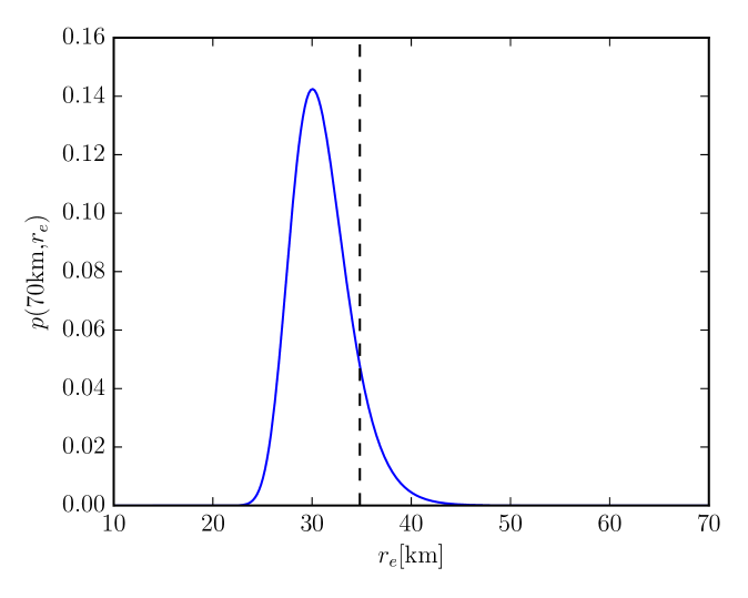
Figure 1: The probability that neutrino with energy 10 MeV observed at the distance $r=70$ km from the centre of a star is emitted at the distance $r_{e}$. We use the density distribution from Eq. (2.8), the electron fraction $Y_{e}=0.4$ and the temperature profile in Eq. (2.9). The dashed line indicates the position of the infinitesimal neutrino sphere according to Eq. (1.1).

2.2 Effect of averaging over the neutrino production region

We consider the system of two mixed neutrinos $\nu_{f}=(\nu_{e},\nu_{x})$, where $\nu_{x}$ is a linear combination of $\nu_{\mu}$ and $\nu_{\tau}$. As the mass squared difference, we take $\Delta m^{2}=\Delta m_{31}^{2}$. The wave function describing the neutrino flavour $\psi\equiv(\psi_{e},\psi_{\mu})^{T}$ evolves according to the equation

$$i\partial_{r}\psi(r)=H(r)\psi(r)$$ (2.10)

with the Hamiltonian

$$H(r)=\frac{1}{2}\begin{pmatrix}-\omega\cos 2\theta+V_{e}(r)&\omega\sin 2\theta\\ \omega\sin 2\theta&\omega\cos 2\theta-V_{e}(r)\end{pmatrix}.$$ (2.11)

Here $\omega\equiv\Delta m^{2}/2E$, $\theta$ is the vacuum mixing angle, and $V_{e}(r)=\sqrt{2}G_{F}(n^{\rm tot}_{e^{-}}(r)-n^{\rm tot}_{e^{+}}(r))$ is the standard matter potential given by the forward neutrino scattering on electrons and positrons.

We introduce the instantaneous eigenstates of the Hamiltonian $\nu^{\prime}\equiv(\nu_{1}^{\prime},\leavevmode\nobreak\ \nu_{2}^{\prime})^{T}$ which diagonalise $H(r)$:

$$\nu_{f}=U(\theta_{m})\nu^{\prime},\leavevmode\nobreak\ \leavevmode\nobreak\ \leavevmode\nobreak\ \leavevmode\nobreak\ U(\theta_{m})^{\dagger}HU(\theta_{m})=H^{\prime},$$ (2.12)

where $U(\theta_{m})$ is the unitary mixing matrix and $\theta_{m}(r)$ is the mixing angle in matter:

$$\sin 2\theta_{m}=\frac{\sin 2\theta}{\sqrt{(\cos 2\theta-V_{e}/\omega)^{2}+\sin^{2}2\theta}}\approx\sin 2\theta\frac{\omega}{V_{e}},$$ (2.13)

and

$$H^{\prime}(r)=\frac{\omega_{m}(r)}{2}\begin{pmatrix}-1&0\\ 0&1\end{pmatrix}$$ (2.14)

is the Hamiltonian in the basis of instantaneous eigenstates with $\omega_{m}(r)$ being the difference of the eigenvalues or the oscillation frequency:

$$\omega_{m}(r)=\omega\sqrt{(\cos 2\theta-V_{e}/\omega)^{2}+\sin^{2}2\theta}.$$

In central parts of the supernova, the adiabaticity condition,

$$\gamma_{ad}\equiv\frac{1}{\omega_{m}(r)}\frac{d\theta_{m}(r)}{dr}\ll 1,$$

is well satisfied. E.g., for the density profile in Eq. (2.8), we find $\gamma_{ad}=10^{-17}$ and $\gamma_{ad}=10^{-8}$ for $r=50$ and $200$ km respectively. Therefore, there are no transitions between the eigenstates, and they evolve independently:

$$\psi_{1}^{\prime}\propto\exp\left[\frac{1}{2}i\int\omega_{m}(r)dr\right],\leavevmode\nobreak\ \leavevmode\nobreak\ \leavevmode\nobreak\ \psi_{2}^{\prime}\propto\exp\left[-\frac{1}{2}i\int\omega_{m}(r)dr\right].$$ (2.15)

In the basis of eigenstates, the electron neutrino is described by

$$\psi_{e}(r)=\begin{pmatrix}\cos\theta_{m}(r)\\ \sin\theta_{m}(r)\end{pmatrix}.$$ (2.16)

Then the evolution of a state produced as $\nu_{e}$ is, according to (2.15), given by

$$\psi_{e}(r)=\begin{pmatrix}\cos\theta_{m}(r_{e})e^{0.5i\int\omega_{m}(r)dr}\\ \sin\theta_{m}(r_{e})e^{-0.5i\int\omega_{m}(r)dr}\end{pmatrix},$$ (2.17)

where the $\theta_{m}(r_{e})$ is the mixing angle in the production point.

Let us introduce the correlation of the eigenstates in the state produced as $\nu_{e}$:

$$\rho_{12}^{\prime}(r)=\psi^{\prime}_{1}(r)\psi^{\prime*}_{2}(r).$$ (2.18)

It is this correlation given by the off-diagonal element of the density matrix that is responsible for flavour conversion. According to (2.17)

$$\rho_{12}^{\prime}(r,r_{e})=\frac{1}{2}\sin 2\theta_{m}(r_{e})\exp\left(i\int_{r_{e}}^{r}\omega_{m}(r^{\prime})dr^{\prime}\right).$$ (2.19)

The correlation averaged over the neutrino production region equals

$$\left<\rho_{12}^{\prime}(r)\right>=\int_{0}^{r}p(r,r_{e})\frac{1}{2}\sin 2\theta_{m}(r_{e})\exp\left(i\int_{r_{e}}^{r}\omega_{m}(r^{\prime})dr^{\prime}\right)dr_{e},$$ (2.20)

where the emission probability $p(r,r_{e})$ is determined in Eq. (2.7). From Eq. (2.20), we can immediately see two properties of the averaged correlation:

1. The exponent introduces very fast oscillations, and this results in a strong suppression of the integral over $r_{e}$ (as it was noticed in [3]).

2. The emission probability $p(r,r_{e})$ decreases with $J\propto n_{e}n_{N}$ at large radii while $\sin 2\theta_{m}$ increases as $1/V_{e}\sim 1/n_{e}$ (for $V_{e}\gg\omega$) partially cancelling the dependence on $r_{e}$ in the integrand. Although the dependence on $n_{e^{-}}^{\rm tot}$ cancels, there is still a decrease of the integrand with $r_{e}$ due to the Boltzmann factor and the number density of nucleons.

For the exponential density profile in Eq. (2.8) and the temperature profile in Eq. (2.9), the averaging in Eq. (2.20) can be performed analytically when the Boltzmann suppression of $n_{e}(E,r)$ is neglected. For $r\gg r_{0}$ using that $\sigma_{\rm nucleon}n_{N}(r_{0})r_{0}\gg 1$, we obtain

$$\left<\rho_{12}^{\prime}(r)\right>\approx-i\frac{1}{2}\sin 2\theta_{m}\frac{1}{r_{0}V_{e}}\frac{r_{0}^{2}}{l_{\rm abs}^{2}},$$ (2.21)

where $l_{\rm abs}\equiv(\sigma_{\rm nucleon}n_{n})^{-1}$ is the neutrino absorption length and $r_{0}$ is defined below Eq. (2.8). (The oscillatory terms in $\left<\rho_{12}^{\prime}(r)\right>$ are suppressed by $e^{-\sigma n_{0}r_{0}}$.) According to (2.21), apart from very small $\sin 2\theta_{m}$, the correlation contains an additional suppressed factor $r_{\rm eff}V_{e}$ where $r_{\rm eff}=l_{\rm abs}^{2}/r_{0}$. The effective width of the production region is determined by the absorption length, so that averaging becomes weaker with the decrease of $l_{\rm abs}$. Numerically, $l_{\rm abs}\sim 5$ km for $n_{N}\sim 2\times 10^{35}{\rm cm}^{-3}$ which corresponds to $r\sim 35$ km for the density profile in Eq. (2.8). The dependence on radius in $\sin 2\theta_{m}$, $V_{e}$, and $l_{\rm abs}$ cancels in Eq. (2.21), so these three quantities can be evaluated at any radius as long as it is the same for all three.

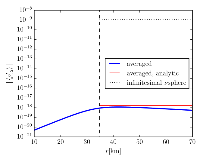
Figure 2: The averaged correlation in the eigenstates basis as function of the distance from the centre of the star. Shown are results of the numerical integration in Eq. (2.20) (blue line) and the analytic result in Eq. (2.21) (red line). In the calculations, the emission probability of Figure 1 is used. The neutrino energy is 10 MeV and the electron fraction is assumed to be $Y_{e}=0.4$. For comparison we show the result for a neutrino sphere of infinitesimal width at $r_{e}=35$ km as the dotted line.

The results of the numerical evaluation of the averaged correlation in Eq. (2.20) is shown in Figure 2 together with the analytical estimation from Eq. (2.21). The vertical dashed line indicates the position of the infinitesimal neutrino sphere from Eq. (1.1). The difference between the numerical and analytic result is due to the neglected Boltzmann suppression in the analytic calculation. Notice that the initial increase of $|\left<\rho^{\prime}_{12}\right>|$ is due to contributions from neutrinos emitted at the largest $r_{e}$ (smallest density) since the effective mixing angle increases with the decrease of density.

We see that the integration over the production region leads to a suppression of the off-diagonal term in the density matrix by $\sim 10$ orders of magnitude with respect to the result for an infinitesimal neutrino sphere. Similar suppression of the order $1/V_{e}r_{\rm eff}$ is realised for steeper density profiles with $R_{\nu\rm sphere}=(10-20)$ km. This suppression factor should be included in the initial condition for further collective oscillations. We will justify the factorisation of averaging in the production region and collective oscillations outside the production region later using a solvable example.

3 Averaging in the presence of $\nu\nu$ interactions

3.1 Model with $\nu\nu$ interactions

In order to understand how the emission of neutrinos from different points influences collective oscillations, we will consider the simple system with neutrino self-interactions, two intersecting fluxes of collinear neutrinos moving in the plane $(x,z)$ [14, 15, 16, 17, 18, 19]. The fluxes have angles $\beta$ (right moving) and $\pi-\beta$ (left moving) with respect to the $x$-axis (the same angles with respect to $z$). Both fluxes contain equal number densities of neutrinos and antineutrinos and all neutrinos have the same vacuum frequency $\omega$. The fluxes are moving in a uniform medium with matter potential $V_{e}$. We consider the production of electron (anti)neutrinos only.

The set-up is symmetric with respect to the reflection $\beta\rightarrow\pi-\beta$, and therefore left and right moving neutrinos have the same evolution.

We took equal numbers of neutrinos and antineutrinos for simplicity. This is the most favourable case for collective oscillations where bi-polar oscillations can start immediately without a delay. We assume that the neutrinos are produced in a region of width $\Delta z$, so that the coordinates of production points $z_{e}$ are in the interval $0\leq z_{e}\leq\Delta z$. In this model the time (distance) of propagation along the trajectory is uniquely related to the coordinate $z$:

$$t=t(z)=\frac{z}{s_{\beta}},\leavevmode\nobreak\ \leavevmode\nobreak\ \leavevmode\nobreak\ dt=\frac{1}{s_{\beta}}dz,\leavevmode\nobreak\ \leavevmode\nobreak\ \leavevmode\nobreak\ \leavevmode\nobreak\ s_{\beta}\equiv\sin\beta,$$

and in what follows, we will use $z$ to describe the evolution.

We will treat the problem in terms of density matrices $\rho(z_{e},z)$ and $\bar{\rho}(z_{e},z)$ which describe the state of neutrinos and antineutrinos produced as $\nu_{e}$ and $\bar{\nu}_{e}$ at $z_{e}$ as a function of coordinate $z$. The evolution equation for $\rho(z_{e},z)$ in the flavour basis is

$$is_{\beta}\frac{d}{dz}\rho(z_{e},z)=[H(z),\rho(z_{e},z)],$$ (3.1)

where

$$H(z)=\frac{\omega}{2}\begin{pmatrix}-\cos 2\theta&\sin 2\theta\\ \sin 2\theta&\cos 2\theta\end{pmatrix}+\frac{1}{2}\begin{pmatrix}V_{e}&0\\ 0&-V_{e}\end{pmatrix}+\mu\int_{0}^{z}\left[\rho(z_{e}^{\prime},z)-\bar{\rho}^{*}(z_{e}^{\prime},z)\right]p_{\nu}(z_{e}^{\prime})dz_{e}^{\prime}.$$ (3.2)

Here $p_{\nu}(z_{e}^{\prime})$ is the probability that a given free streaming neutrino is produced at the point $z_{e}^{\prime}$ and $\mu=\sqrt{2}G_{F}n_{\nu}$, where $n_{\nu}=n_{\nu_{e}}-n_{\nu_{x}}$ is the effective density of neutrinos at $z>\Delta z$, so $\mu$ is the total potential produced by the neutrino background outside the production region. The first and second terms in Eq. (3.2) coincide with the Hamiltonian in (2.11), the last term is due to $\nu\nu$ interactions. We take equal numbers of neutrinos and antineutrinos, so that ${\rm Tr}(\rho)={\rm Tr}(\bar{\rho})=1$. We assume the hierarchy of frequencies

$$V_{e}\gg\mu\gg|\omega|$$

typical for the central parts of supernovae.

In the Hamiltonian for antineutrinos, $V_{e}$ has the opposite sign, and $\rho$ and $\bar{\rho}$ are swapped. The initial condition reads $\rho_{ee}=\bar{\rho}_{ee}=1$.

For simplicity, we assume that neutrinos are produced in the layer $z\in[0,\Delta z]$ uniformly, so that the emission probability introduced in the previous section equals

$$p_{\nu}(z_{e})=\begin{cases}\frac{1}{\Delta z}&{\rm for}\quad 0<z_{e}<\Delta z,\\ 0&{\rm otherwise}\end{cases}.$$ (3.3)

In contrast to the previous section, we impose the size $\Delta z$ by hand.

With the emission profile (3.3) and a constant matter density, the expression Eq. (2.20), where $\nu\nu$ interactions are not accounted for, is simplified for $z>\Delta z$:

$$\left<\rho_{12}^{\prime}(z)\right>=\frac{1}{2\Delta z}\sin 2\theta_{m}\int_{0}^{\Delta z}\exp\left[i\omega_{m}(z-z_{e})/s_{\beta}\right]dz_{e}$$ (3.4)

if the neutrino background contribution is neglected in $\theta_{m}$ and $\omega_{m}$. Furthermore, since $\mu,\omega\ll V_{e}$, we can neglect $\mu$ and $\omega$ in $\omega_{m}$, so that $\omega_{m}\approx V_{e}$ and integration in (3.4) can be performed explicitly giving

$$|\left<\rho_{12}^{\prime}(z)\right>|=\frac{s_{\beta}\sin 2\theta_{m}}{V_{e}\Delta z}$$ (3.5)

for the phase $\pi+2\pi k$. Thus, as expected, integration leads to additional suppression of the correlation by a factor $(V_{e}\Delta z)^{-1}\ll 1$.

Throughout the emission region, the number of neutrinos increases as more neutrinos are emitted. The fraction of neutrinos that has been emitted by a given point z equals

$$f_{\nu}(z)=\int_{0}^{z}p_{\nu}(z_{e})dz_{e}=\begin{cases}\frac{z}{\Delta z}&{\rm for}\quad 0<z<\Delta z,\\ 1&{\rm for}\quad z>\Delta z.\end{cases}$$ (3.6)

Then the potential due to the neutrino background can be parametrised as

$$\tilde{\mu}(z)=\mu f_{\nu}(z)$$ (3.7)

which is the fraction of the potential due to $\nu\nu$ interactions accumulated to a given point $z$. For our model of emission (3.6):

$$\tilde{\mu}(z)\equiv\begin{cases}\mu\frac{z}{\Delta z}&{\rm for}\quad 0<z<\Delta z,\\ \mu&{\rm for}\quad z>\Delta z.\end{cases}$$ (3.8)

We are interested in the evolution of flavour of the entire ensemble of neutrinos. Therefore, we define the total normalised density matrix as

$$\rho^{\rm int}(z)=\frac{1}{f_{\nu}(z)}\int_{0}^{z}\rho(z_{e},z)dz_{e}.$$ (3.9)

The density matrix $\rho^{\rm int}$ is normalised in the same way as a single state. So in what follows, we will talk about averaging of the density matrix over the production region.

3.2 Results of numerical computations

We will study averaging effects depending on the width of the production region $\Delta z$. Since the total number of emitted neutrinos $\mu$ is fixed, the emissivity decreases with the increase of $\Delta z$. To see 10 orders of magnitude suppression in a numerical computations, about $\mathcal{O}(10^{10})$ different emission points have to be included, which is unfeasible. Therefore, we use a much weaker hierarchy between the different frequencies involved and assume a size of the emission region which is at most a few orders of magnitude larger than the oscillation length. We take the inverted hierarchy, $\omega<0$, and for definiteness the following values of parameters:

$$V_{e}=30|\omega|,\leavevmode\nobreak\ \leavevmode\nobreak\ \leavevmode\nobreak\ \mu=3|\omega|,\leavevmode\nobreak\ \leavevmode\nobreak\ \leavevmode\nobreak\ \theta=0.15,\leavevmode\nobreak\ \leavevmode\nobreak\ \leavevmode\nobreak\ \leavevmode\nobreak\ \beta=\pi/4.$$ (3.10)

We solve the evolution equations numerically to obtain $\rho(z_{e},z)$ and $\rho^{\rm int}$. Details of our computations are given in Appendix A. (Although $s_{\beta}=1/\sqrt{2}$, we will still keep $s_{\beta}$ in formulas below.)

The result of averaging depends on the exact value of $\Delta z$. For definiteness, we will take $\Delta z$ to be semi-integer numbers of matter refraction lengths $2\pi/V_{e}$: $\Delta z=(2n+1)\pi s_{\beta}/V_{e}$, where $n\geq 0$ is an integer. Due to the presence of neutrinos in the background, this does not correspond exactly to a semi-integer number of oscillations. Numerically, for values of parameters (3.10) we have $\Delta z|\omega|=0.074(2n+1)$. The results of computations are shown in Figure 3 for relatively narrow production regions: $n=1,\leavevmode\nobreak\ 3,\leavevmode\nobreak\ 10$, which corresponds to $\Delta z|\omega|<1.5$, and in Figure 4 for the wider regions with $n=80,\leavevmode\nobreak\ 120,\leavevmode\nobreak\ 160$ ($\Delta z|\omega|>12$). For comparison, we also present results for a surface emission at $z=0$ with $\Delta z=0$.

The upper panels show, as expected, a gradual delay of the oscillations of $\rho_{ee}$ with an increase of the emission region. $\rho_{ee}\approx 1$ in the initial phase, and then the evolution proceeds with bi-polar oscillations. In Figure 3, the strong transition effect develops outside the production region. Consequently, the depth and the period of oscillations do not depend on $\Delta z$. The only effect of the averaging is a delay of the strong transition – a shift of the first minimum. The exponential growth is the same for all $\Delta z$ at $z>\Delta z$. For large values of $\Delta z$ ($n=80$, $120$, and $160$), strong conversion develops already within the emission region.

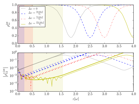
Figure 3: The elements of density matrices averaged over narrow production regions as functions of the distance from the beginning of the region for different values of width $\Delta z$ (shadowed). Upper panel: The $\nu_{e}$ survival probability ($\rho_{ee}$). Bottom panel: The correlation – the off-diagonal term of the density matrix in the eigenstates basis $\rho_{12}$. Thick lines show analytic results based on the solution of the linearised equations.

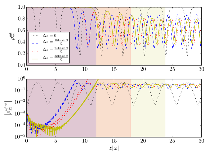
Figure 4: The same as in Figure 3, but for wide production regions.

Although initially, $\rho_{ee}\approx 1$, and no change is seen, important dynamics occurs in this initial phase which eventually leads to the delay of visible bi-polar oscillations. This can be seen and understood in detail in terms of the correlation of the eigenstates $\rho_{12}$ (2.18).

Eqs. (3.1) and (3.2) and the corresponding density matrices are given in the flavour basis. To explore the correlations $\rho_{12}$, we need to make a transformation to the eigenstate basis. The relation between the off-diagonal elements of the density matrices in the flavour and eigenstates bases (see Appendix B) is given by

$$\left|\rho_{12}^{\nu,{\rm int}}(z)\right|\approx\left|\rho_{ex}^{{\rm int}}(z)-\frac{\omega\sin 2\theta}{2(V_{e}-\omega\cos 2\theta)}\left(1+2\frac{\tilde{\mu}(z)}{V_{e}}\right)\right|,$$ (3.11)

where $\tilde{\mu}(z)$ is defined in (3.8). Thus, the transition to the eigenstate basis adds a small term which becomes negligible in the period of strong collective effects. So, apart from the initial phase of evolution, when $\rho_{ex}\approx 0$, we have

$$|\rho^{\nu}_{12}|\approx|\rho_{ex}|,\leavevmode\nobreak\ \leavevmode\nobreak\ \leavevmode\nobreak\ \leavevmode\nobreak\ |\rho_{ex}|=\sqrt{\rho_{ee}(1-\rho_{ee})}.$$ (3.12)

The results of evolution of $\rho_{12}^{\nu,\rm int}$ are shown in the lower panels of Figure 3 and Figure 4. According to the figures (bottom panel), there are two benchmark points:

• $z_{0}$ – The point of onset of the exponential growth of the correlation due to collective effects.

• $z_{1}$ – The coordinate at which maximum of the correlation defined by the condition $|\langle\rho_{12}^{\nu,\rm int}(z_{1})\rangle|\sim 0.5$ is achieved for the first time.

Correspondingly, one can identify three phases of the evolution:

• $z\in[0,z_{0}]$ – The averaging phase when the correlation $|\langle\rho_{12}^{\nu,\rm int}\rangle|$ decreases due to integration over the production region and collective effects can be neglected;

• $z\in[z_{0},z_{1}]$ – Nearly exponential growth of the correlation $|\langle\rho_{12}^{\nu,\rm int}\rangle|$; here collective effects start to dominate.

• $z>z_{1}$ – Regular (or quasi-regular) bi-polar oscillations.

The difference of frequencies for different sizes of the production region that can be seen in Figure 4 is related to a difference in neutrino densities since the density equals $n^{\rm tot}z/\Delta z$ in our model, and the total number density of neutrinos outside the production region, $n^{\rm tot}$, is the same for all widths. So the bigger the production region, the smaller the neutrino density, and the smaller the frequency as can be seen in Figure 4 (upper panel). Outside the production regions, all frequencies are equal. (The only exception is $\Delta z=0$ for which the flavour evolution takes the system very close to the ’fixed point’ at $\rho^{\nu}_{12}=0$ ($\rho_{ee}\approx 1$), where the flavour only changes slowly. This delays the oscillations and gives a significantly lower frequency.)

In our model with increasing $\tilde{\mu}$ in the emission region, the onset of collective effects is always in the emission region: $z_{0}\leq\Delta z$. Depending on the size of $\Delta z$ with respect to $z_{1}$, there are two different situations:

1. Narrow production region: $\Delta z<z_{1}$. The instability develops partly outside the production region (Figure 3). In this case for $z>z_{1}$, oscillations proceed with constant parameters (depth and period). Furthermore, $\rho_{ee}=1$ at the maxima. So the asymptotic behaviour starts from $z_{1}$.

   If the production region is very narrow, $\Delta z\ll z_{1}$, we can neglect effect of collective oscillations in the emission region and consider the exponential growth only outside this region with certain boundary conditions. The description is further simplified in this case. That would correspond to the situation described in Section 2.

2. Wide production region: $\Delta z>z_{1}$. In this case the instability (with exponential growth) develops completely inside the production region (see Figure 4). In the interval after the development of the instability between $z_{1}$ and $\Delta z$, bi-polar oscillations proceed with decreasing depth, and asymptotic oscillations start from $z_{\rm as}=\Delta z$.

   The off-diagonal term in the density matrix peaks twice before it starts to decrease again. The maximal value of $\rho^{\nu}_{12}$ (maximal possible correlation between the two eigenstates) is achieved when $\rho_{ee}^{\rm int}\sim 0.5$, as can be seen from Eq. (3.12).

In what follows, we will consider these two possibilities separately. Notice that for the adiabatic propagation, $|\rho^{\nu}_{12}|=$ constant, and therefore changes of $|\rho^{\nu}_{12}|$ reflect adiabaticity violation or new neutrinos joining the system.

4 Analytic consideration using linearised equations

As it follows from Fig. 3, the exponential growth of the off-diagonal elements of $\rho^{\nu}$ with $z$ starts when $\rho^{\nu}_{12}\ll 1$ and proceeds until $\rho^{\nu}_{12}\sim 0.3$. In this range of $z$, one can use linearised equations of evolution which allow us to solve the problem analytically. The rate of exponential growth of $\rho^{\nu}_{12}$ can be calculated through linear stability analysis [20]. The analysis is based on linearised evolution equations for the off-diagonal part of the density matrix.

The linear analysis has to be performed around a ’fixed point’ – that is a point in the space of density matrices where $d\rho/dz=0$ to zeroth order in the small off-diagonal element, and evolution only starts at linear or higher order. We find such a fixed point in the basis of propagating states where a vanishing off-diagonal term in the density matrix corresponds to independently propagating states with no oscillations.

We consider density matrices of neutrinos and antineutrinos produced as $\nu_{e}$ and $\bar{\nu}_{e}$ at $z_{e}$. In the case of adiabatic evolution, the basis of propagating states approximately coincide with the eigenstate basis – the basis of eigenstates of the instantaneous Hamiltonian where the $\nu\nu$ interaction term is included. For the calculations, we use the eigenstate basis (see Appendix C for details). Since the matrices have trace 1, we can present them in the eigenstate basis as

$$\rho^{\nu}(z_{e},z) =\frac{1}{2}\begin{pmatrix}1&0\\ 0&1\end{pmatrix}+\frac{1}{2}\begin{pmatrix}-s(z_{e},z)&-S^{*}(z_{e},z)\\ -S(z_{e},z)&s(z_{e},z)\end{pmatrix},$$ (4.1)

$$\bar{\rho}^{\nu}(z_{e},z) =\frac{1}{2}\begin{pmatrix}1&0\\ 0&1\end{pmatrix}+\frac{1}{2}\begin{pmatrix}\bar{s}(z_{e},z)&\bar{S}^{*}(z_{e},z)\\ \bar{S}(z_{e},z)&-\bar{s}(z_{e},z)\end{pmatrix},$$

for $0<z_{e}<\Delta z$. For $z_{e}>\Delta z$, $\rho^{\nu}(z_{e},z)=\bar{\rho}^{\nu}(z_{e},z)=0$. The traces play no role in the evolution equation, and furthermore, $s^{2}+S^{2}=1$. In the limit $V_{e}\gg\omega$ in the neutrino emission region, we have $S\ll 1$, and therefore $s=1$ ($\bar{s}=1$) to first order in $S$ ($\bar{S}$). At the production point $S=-\sin 2\theta_{\nu}$ and $\bar{S}=\sin 2\theta_{\bar{\nu}}$.

4.1 Equations for the integrated $S$

Using (3.2) and (3.1), we can derive the Hamiltonian and the evolution equation for the density matrix in the eigenstate basis (see Appendix C for more details). Inserting the expressions from (4.1), we get the following equations to lowest order in $S$ and $\bar{S}$

$$is_{\beta}\frac{d}{dz}S(z_{e},z) =\left(-\omega+V_{e}\right)S(z_{e},z)+\mu\int_{0}^{z}p_{\nu}(z_{e}^{\prime})\left[\bar{S}(z_{e}^{\prime},z)-S(z_{e}^{\prime},z)\right]dz_{e}^{\prime},$$ (4.2)

$$is_{\beta}\frac{d}{dz}\bar{S}(z_{e},z) =\left(\omega+V_{e}\right)\bar{S}(z_{e},z)+\mu\int_{0}^{z}p_{\nu}(z_{e}^{\prime})\left[\bar{S}(z_{e}^{\prime},z)-S(z_{e}^{\prime},z)\right]dz_{e}^{\prime}.$$

Eqs. (4.2) is a system of two coupled equations for the neutrino and antineutrino modes. Notice that the evolution equation for $\rho^{\nu}$ derived from (3.1) gives two connected equations for $S$ and $S^{*}$ which are equivalent, as a result of $\rho=\rho^{\dagger}$. The same holds for $\bar{\rho}$. Consequently, we have only two equations in the neutrino-antineutrino system instead of four.

We will search for a solution for the individual modes (produced at $z_{e}$) in the form

$$\begin{pmatrix}S(z_{e},z)\\ \bar{S}(z_{e},z)\end{pmatrix}=\exp\left(-is_{\beta}^{-1}\int_{z_{e}}^{z}\Omega(z^{\prime})dz^{\prime}\right)\begin{pmatrix}Q(z_{e})\\ \bar{Q}(z_{e})\end{pmatrix}$$ (4.3)

with the integral in the exponent. Inserting (4.3) into (4.2), we find

$$\left[\Omega(z)+\omega-V_{e}\right]e^{-is_{\beta}^{-1}\int_{z_{e}}^{z}\Omega(z^{\prime})dz^{\prime}}Q(z_{e}) =\mu\int_{0}^{z}p(z_{e}^{\prime})e^{-is_{\beta}^{-1}\int_{z_{e}^{\prime}}^{z}\Omega(z^{\prime\prime})dz^{\prime\prime}}\left[\bar{Q}(z_{e}^{\prime})-Q(z_{e}^{\prime})\right]dz_{e}^{\prime},$$ (4.4)

$$\left[\Omega(z)-\omega-V_{e}\right]e^{-is_{\beta}^{-1}\int_{z_{e}}^{z}\Omega(z^{\prime})dz^{\prime}}\bar{Q}(z_{e}) =\mu\int_{0}^{z}p(z_{e}^{\prime})e^{-is_{\beta}^{-1}\int_{z_{e}^{\prime}}^{z}\Omega(z^{\prime\prime})dz^{\prime\prime}}\left[\bar{Q}(z_{e}^{\prime})-Q(z_{e}^{\prime})\right]dz_{e}^{\prime}.$$

The integrated and normalised element $S^{\rm int}$ equals

$$S^{\rm int}(z)=\frac{1}{f_{\nu}(z)}\int_{0}^{z}p(z_{e})S(z_{e},z)dz_{e}=\frac{1}{f_{\nu}(z)}\int_{0}^{z}p(z_{e})e^{-is_{\beta}^{-1}\int_{z_{e}}^{z}\Omega(z^{\prime})dz^{\prime}}Q(z_{e})dz_{e},$$ (4.5)

and a similar expression, $\bar{S}^{\rm int}(z)$, can be written for antineutrinos. Multiplying Eqs. (4.4) by $p(z_{e})/f_{\nu}(z)$ and integrating over $z_{e}$, we obtain equations for the integrated modes (4.5), which can be expressed as

$$\begin{pmatrix}-\omega+V_{e}-\tilde{\mu}-\Omega&\tilde{\mu}\\ -\tilde{\mu}&\omega+V_{e}+\tilde{\mu}-\Omega\end{pmatrix}\begin{pmatrix}S^{\rm int}\\ \bar{S}^{\rm int}\end{pmatrix}=0,$$ (4.6)

where $\tilde{\mu}(z)$ was defined in Eq. (3.7) and (3.8). A non-trivial solution of the system of linear equations in Eq. (4.6) for $S^{\rm int}$ exists if the determinant of the matrix in (4.6) is zero. This gives the expression

$$\Omega(z)=V_{e}\pm\sqrt{\omega(2\tilde{\mu}(z)+\omega)}.$$ (4.7)

The key feature of (4.2) is that it is anti-symmetric and nontrivial evolution occurs due to couplings of neutrinos and antineutrinos given by $\mu$. Without $\nu\nu$ interactions ($\tilde{\mu}=0$), the equations decouple.

The exponentially growing collective mode appears when ${\rm Im}(\Omega)>0$. Since $\tilde{\mu}$ is positive, this leads to the conditions

$$2\tilde{\mu}>|\omega|,\leavevmode\nobreak\ \leavevmode\nobreak\ \leavevmode\nobreak\ \leavevmode\nobreak\ {\rm for}\leavevmode\nobreak\ \leavevmode\nobreak\ \leavevmode\nobreak\ \leavevmode\nobreak\ \omega<0.$$ (4.8)

The equality $\tilde{\mu}(z_{0})=|\omega|/2$ determines the coordinate of the onset of collective oscillations:

$$z_{0}=\Delta z\frac{|\omega|}{2\mu}.$$ (4.9)

At this $z$, the exponential growth of the correlation starts. Here we used the explicit expression for $\tilde{\mu}(z_{0})$ (3.8). In terms of $z_{0}$, we can write $\sqrt{|\omega|(2\mu-|\omega|)}=|\omega|\sqrt{z/z_{0}-1}$. The normalisation factors $Q(z_{e})$ and $\bar{Q}(z_{e})$ are determined by the initial conditions $Q(z_{e})=S(z_{e},z=z_{e})$ and $\bar{Q}(z_{e})=\bar{S}(z_{e},z=z_{e})$. Since electron neutrinos are produced, we find that

$$-Q(z_{e})\approx\bar{Q}(z_{e})\approx 2\rho^{\nu}_{12}(z_{e})\approx\sin 2\theta_{m}\approx\frac{\omega\sin 2\theta}{V_{e}},$$ (4.10)

and they weakly depend on $z_{e}$. (The dependence arise due to $\tilde{\mu}(z)$ and it disappears if $\tilde{\mu}(z)$ is neglected in comparison to $V_{e}$.)

Thus, the solution (4.5) equals approximately

$$S^{\rm int}(z)=-\frac{\sin 2\theta_{m}}{f_{\nu}(z)}\int_{0}^{z}p(z_{e})e^{-is_{\beta}^{-1}\int_{z_{e}}^{z}\Omega(z^{\prime})dz^{\prime}}dz_{e},$$ (4.11)

where $\Omega(z)$ is determined in (4.7). In terms of the onset parameter $z_{0}$ from (4.9), $\Omega(z)$ can be written as

$$\Omega(z)=V_{e}+\frac{|\omega|}{\sqrt{z_{0}}}\begin{cases}(z_{0}-z)^{1/2}&{\rm for}\quad 0<z<z_{0},\\ i(z-z_{0})^{1/2}&{\rm for}\quad z_{0}<z<\Delta z,\\ i(\Delta z-z_{0})^{1/2}&{\rm for}\quad z>\Delta z.\end{cases}$$ (4.12)

Integration of $\Omega$ in the exponent of (4.11) can be done explicitly:

$$\frac{1}{s_{\beta}}\int_{z_{e}}^{z}\Omega(z^{\prime})dz^{\prime}=\frac{1}{s_{\beta}}\left[V_{e}(z-z_{e})+I(z,z_{e})\right].$$ (4.13)

The integral $I(z,z_{e})$ splits into $z$- dependent and $z_{e}$-dependent parts:

$$I(z,z_{e})=I(z)+I(z_{e}).$$ (4.14)

Taking into account that $\Omega(z)$ has different expressions in different ranges of $z$, we find that there are four possibilities depending on the relative values of $z$, $z_{e}$, $z_{0}$ and $\Delta z$. In all the cases we will take $z>z_{0}$.

1. $z<\Delta z$ (wide emission region), $z_{e}<z_{0}$: Integration proceeds in two intervals $[z_{e},z_{0}]$ and $[z_{0},z_{e}]$ giving

   $$I(z,z_{e})=I_{W}(z)+I_{b}(z_{e}),$$

   where

   $$I_{W}(z)=i\frac{2}{3}\frac{|\omega|}{\sqrt{z_{0}}}(z-z_{0})^{3/2},$$ (4.15)

   $$I_{b}(z_{e})=\frac{2}{3}\frac{|\omega|}{\sqrt{z_{0}}}(z_{0}-z_{e})^{3/2}$$ (4.16)

2. $z<\Delta z$, $z_{e}>z_{0}$: Integration is over a single interval $[z_{e},z]$ with the result

   $$I(z,z_{e})=I_{W}(z)+I_{a}(z_{e}),$$

   where $I_{W}(z)$ is the same as in (4.15), and

   $$I_{a}(z_{e})=-i\frac{2}{3}\frac{|\omega|}{\sqrt{z_{0}}}(z_{e}-z_{0})^{3/2}.$$ (4.17)

3. $z>\Delta z$ (narrow emission region), $z_{e}<z_{0}$:

   $$I(z,z_{e})=I_{N}(z)+I_{b}(z_{e}).$$

   Here $I_{b}(z_{e})$ is given in (4.16), and $I_{N}(z)$ is the result of integration over two intervals $[z_{0},\Delta z]$ and $[\Delta z,z]$:

   $$I_{N}(z)=i\frac{2}{3}\frac{|\omega|}{\sqrt{z_{0}}}\left[(\Delta z-z_{0})^{3/2}+\frac{3}{2}(\Delta z-z_{0})^{1/2}(z-\Delta z)\right].$$ (4.18)

4. $z>\Delta z$, $z_{e}>z_{0}$:

   $$I(z,z_{e})=I_{N}(z)+I_{a}(z_{e})$$

   with $I_{N}(z)$ and $I_{a}(z_{e})$ defined in (4.18) and (4.17) respectively.

Using the expressions (4.13) and (4.14) and $p_{\nu}$ from (3.3), the solution (4.11) can be written as

$$S^{\rm int}(z)=-\frac{\sin 2\theta_{m}}{\Delta zf_{\nu}(z)}e^{-i[V_{e}z+I(z)]/s_{\beta}}\int_{0}^{z_{\rm max}}dz_{e}e^{-i[V_{e}z_{e}+I(z_{e})]/s_{\beta}},$$ (4.19)

where $z_{\rm max}=z$ for a wide region $z<\Delta z$, and $z_{\rm max}=\Delta z$ for a narrow region. The expressions for $f_{\nu}(z)$ and $I(z)$ should be taken according to the value of $z$.

Since $I(z)$ is purely imaginary, we obtain

$$|S^{\rm int}(z)|=\frac{s_{\beta}\sin 2\theta_{m}}{\Delta zf_{\nu}(z)}|G(z_{\rm max})|e^{-iI(z)/s_{\beta}}.$$ (4.20)

where

$$G(z_{\rm max})\equiv\int_{0}^{z_{\rm max}}\frac{dz_{e}}{s_{\beta}}e^{-i[V_{e}z_{e}+I(z_{e})]/s_{\beta}}.$$ (4.21)

The integral over $dz_{e}$ should be taken on the two intervals $[0,z_{0}]$ and $[z_{0},z_{\rm max}]$. In these intervals, $I(z_{e})$ has the expressions $I(z_{e})=I_{b}(z_{e})$ and $I(z_{e})=I_{a}(z_{e})$ respectively. This integral does not depend on whether the emission region is wide or narrow.

In general, the integral over $z_{e}$ can not be computed analytically, but it can be estimated for negligible $I(z_{e})$ . Averaging over the fast oscillations driven by $V_{e}$, we find for $z\gg z_{0}$

$$|G(z)|=|G(\Delta z)|\approx\frac{1}{V_{e}}.$$ (4.22)

Then the correlation from (4.20) becomes

$$|S^{\rm int}(z)|=\frac{s_{\beta}\sin 2\theta_{m}}{\Delta zf_{\nu}(z)V_{e}}e^{-iI(z)/s_{\beta}}.$$ (4.23)

In what follows, we will consider the correlations in Eq. (4.23) for wide and narrow regions separately and compare them with our numerical results.

4.2 Narrow emission region

In the case of a narrow production region, $\Delta z<z_{1}$, we have $f_{\nu}=1$,

$$|S^{\rm int}(z)|=\frac{s_{\beta}\sin 2\theta_{m}}{\Delta z}|G(\Delta z)|e^{-iI_{N}(z)/s_{\beta}},$$ (4.24)

and the dependence on $z$ is in $I_{N}(z)$ only. Using the expression for $I_{N}(z)$ from (4.18) and $|G(\Delta z)|\approx 1/V_{e}$, we obtain

$$|S^{\rm int}(z)|\approx\frac{s_{\beta}\sin 2\theta_{m}}{\Delta zV_{e}}\exp\left\{\frac{2|\omega|z_{0}}{3s_{\beta}}\left[\left(\frac{\Delta z}{z_{0}}-1\right)^{3/2}+\frac{3\Delta z}{2z_{0}}\left(\frac{\Delta z}{z_{0}}-1\right)^{1/2}\left(\frac{z}{\Delta z}-1\right)\right]\right\}.$$ (4.25)

The first term in the exponent can be written as $2\sqrt{2\mu\omega}\Delta z$. Therefore, for very narrow regions $\Delta z\ll 1/(2\sqrt{2\mu\omega})$, it can be neglected and the solution (4.25) becomes

$$|S^{\rm int}(z)|\approx\frac{s_{\beta}\sin 2\theta_{m}}{\Delta zV_{e}}\exp\left[s_{\beta}^{-1}\sqrt{|\omega|(2\mu-|\omega|)}(z-\Delta z)\right].$$ (4.26)

The correlations $|S^{\rm int}(z)|$ computed with (4.25) for different values of $\Delta z$ are shown in Figure 3. There is a good agreement between the numerical and analytical results. The front factor of Eq. (4.26) coincides with the expression for the averaged $\rho^{\prime}_{12}$ in Eq. (3.5). Hence, the averaging effect can directly be seen in Eq. (4.26) as a reduction of the initial value of $|S^{\rm int}|$ at $z=\Delta z$.

The result in (4.25) can be used in the interval $[\Delta z,z_{1}]$. At $z>z_{1}$, the asymptotic behaviour starts which proceeds in the non-linear regime. It has a form of bi-polar oscillations with constant parameters which can be estimated as follows: For a thin neutrino sphere and a constant value of $\mu$, it was found in [21] that the probability in the oscillation minima equals $P_{ee}^{\rm min}=\omega/2\mu$. At the maxima, $P_{ee}=1$, so that the average equals $P_{ee}=1-\omega/4\mu$. The period of bi-polar oscillations is

$$l_{\rm bp}=2|\ln\theta|\frac{1}{\sqrt{\omega\mu}}.$$ (4.27)

These estimations are in very good agreement with the numerical results in Figure 3.

For a very narrow production region (4.26), the result can be obtained immediately from the corresponding evolution equation. Neglecting collective effects in the emission region, we can consider there the standard oscillations in matter with averaging. This gives the initial condition for further exponential growth which starts at a certain distance $z_{0}^{\prime}$. Therefore, the emission profile is

$$p_{\nu}(z_{e})=\delta(z-z_{0}^{\prime}),$$

so effectively all the neutrino are emitted from the same point $z_{0}^{\prime}$. In this case the neutrino interaction term in the Hamiltonian (3.2) is reduced to $\mu[\rho(z_{0}^{\prime},t)-\bar{\rho}^{*}(z_{0}^{\prime},t)]$. Plugging the matrices from (4.1) into Eqs. (3.1) and (3.2) (and the corresponding equations for antineutrinos) and assuming $\theta\approx 0$, we obtain the following equations for $S$ and $\bar{S}$ to first order in $S$ and $\bar{S}$:

$$is_{\beta}\frac{d}{dz}\begin{pmatrix}S\\ \bar{S}\end{pmatrix}=\begin{pmatrix}-\omega+V_{e}-\mu&\mu\\ -\mu&\omega+V_{e}+\mu\end{pmatrix}\begin{pmatrix}S\\ \bar{S}\end{pmatrix},$$ (4.28)

where $S=S(z_{0}^{\prime},z)$. It can be obtained from (4.6) by replacing $\tilde{\mu}$ by $\mu$. Following the same procedure as before, we arrive at the exponentially growing solution where the values of $Q$ and $\bar{Q}$ are determined by the initial condition which takes into account averaging in the initial phase. $Q(z_{0}^{\prime})=2\langle\rho_{12}^{\prime}(z_{0})\rangle$ and for $|\langle\rho^{\prime}_{12}(z_{0})\rangle|$ we use the result given in (3.5). Finally,

$$\left|\rho_{12}^{\nu,{\rm int}}\right|=\frac{s_{\beta}\sin 2\theta_{m}}{2\Delta zV_{e}}\exp\left[s_{\beta}^{-1}\sqrt{|\omega|(2\mu-|\omega|)}(z-z_{0}^{\prime})\right].$$ (4.29)

For $z_{0}^{\prime}=\Delta z$ this $\rho_{12}$ coincides with the result in (4.26) up to a factor of two that comes from the choice of integration limits for Eq. (3.5).

The very good agreement between the numerical solution and the linear solution demonstrates that the effect of an extended emission region on collective oscillations is well described as an averaging of the initial state.

4.3 Wide emission region

In this case, $\Delta z>z_{1}$, and the instability develops completely inside the emission region. There are three regions of $z$ with different physics: $[0,z_{1}]$, where we can use results of linear approximation; $[z_{1},\Delta z]$, where the evolution becomes non-linear and non-trivial since more neutrinos are emitted and joint the system; $[\Delta z,\infty]$ – where the asymptotics appear.

In the region $z<z_{1}$, we have $f_{\nu}=z/\Delta z$ and according to (4.20),

$$|S^{\rm int}(z)|=\frac{s_{\beta}\sin 2\theta_{m}}{z}|G(z)|e^{-iI_{W}(z)/s_{\beta}}.$$ (4.30)

Here the dependence on $z$ is more complicated: It appears in $I_{W}(z)$, $|G(z)|$ and in the pre-exponential factor. Using expression (4.15) for $I_{W}(z)$ and Eq. (4.22) for $|G(z)|$, we find

$$|S^{\rm int}(z)|\approx\frac{s_{\beta}\sin 2\theta_{m}}{zV_{e}}\exp\left[\frac{2|\omega|z_{0}}{3s_{\beta}}\left(\frac{z}{z_{0}}-1\right)^{3/2}\right].$$ (4.31)

Notice that here the exponential growth is faster than in the case of narrow regions: $\exp(Az^{3/2})$. The reason is that more neutrinos join the system and $\tilde{\mu}$ increases in the range of $z$ where the instability develops. In Figure 4, the analytic results from Eq. (4.31) are shown as bold lines. They agree with the numerical solutions. In particular, Eq. (4.31) captures well the changing slope with $z$ for a given $\Delta z$ as well as the different slopes for different $\Delta z$. Clearly, it is important to use $\tilde{\mu}$ rather than $\mu$.

Some differences between the numerical and analytical results seen in Figure 4 are related to assumptions and approximations involved in deriving Eq. (4.31). In particular,

1. In the ansatz (4.3), we neglected the $z_{e}$ dependence of $Q$. It appears via dependence of mixing on $\tilde{\mu}(z_{e})$.

2. The $z_{e}$-dependent part, $I(z_{e})$, has been neglected in the integral over $z_{e}$ when making the approximation in (4.22).

Both approximations have an accuracy of the order $\mu/V_{e}\sim 10\%$.

Let us consider the evolution in the interval $[z_{1},\Delta z]$ in the non-linear regime but before the system reaches the asymptotics. Here we cannot use the results of the linear approximation. Now the collective oscillations are not as efficient as in the case $z_{1}>\Delta z$. Indeed, according to Figure 4, the depth of the oscillations becomes smaller and the minima become shallower in comparison with the narrow region case.

Generalising the result for the probability at the minimum found in [21] (see Section 4.2), we substitute $\mu$ by $\tilde{\mu}$ in the first oscillation minimum $z_{\rm min}$:

$$\rho_{ee}^{\rm int}(z_{\rm min})\approx\frac{|\omega|}{2\tilde{\mu}(z_{\rm min})}.$$ (4.32)

This expression is in very good agreement with results of numerical computations. The averaged value of $P_{ee}$ decreases, converging to the asymptotic behaviour at $z>\Delta z$, where the oscillations proceed around the average value

$$\langle\rho_{ee,\mathrm{asymptotic}}^{\rm int}\rangle\approx\frac{1}{2}\left(1+\frac{|\omega|}{2\mu}\right)$$ (4.33)

given by the total $\mu$ being independent of the width of the production region.

In order to understand this behaviour, we present results for a very large emission region, $z|\omega|=200$ in Figure 5. In this case, $z_{1}\approx 50$ and the onset coordinate $z_{0}=33$. In the lower panel one sees again a good agreement between the analytic Eq. (4.31) (the dashed line) and the numerical results (the solid line). Furthermore, the value of $\rho_{ee}$ at the minimum is in very good agreement with $\rho_{ee}(z_{\rm min})=0.66$ predicted by Eq. (4.32).

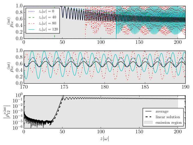
Figure 5: Collective flavour conversion within a very large emission region $\Delta z|\omega|=200$. Upper panel: The $\nu_{e}$ survival probabilities averaged over neutrino production points (solid line) as well as for neutrinos produced in different points as function of distance. Middle panel: A zoom of the probabilities in the range $z|\omega|=170$ to $190$. Bottom panel: The off-diagonal term of the density matrix and the linear solution according to Eq. (4.31). The shading indicates the emission region.

In the upper panel of Eq. (4.32) we show the oscillation probabilities for individual neutrinos emitted at certain points: $z_{e}|\omega|=0,40,80$ and $120$ in addition to the probability averaged over all the neutrinos emitted before a given point $z$.

Neutrinos emitted at 0 and 40, that is in the linear regime $z_{e}<z_{1}$, have almost identical flavour evolutions, and the phases of bi-polar oscillations agree with that of the averaged one. This is essentially the consequence of factorisation of dependencies on $z$ and $z_{e}$, in which all the modes (produced at different $z_{e}$) have the same dependence on $z$ while differences in phases related to $z_{e}$ are encoded in the suppression factor given by the integral $|G(z)|$. So, the phases of their bi-polar oscillations are in a sense synchronised.

Neutrinos produced after $z_{1}$ ($z_{e}>z_{1}$) start the bi-polar oscillations immediately from $z_{e}$. The initial phases of these oscillations are determined by the fact that $\nu_{e}$ and $\bar{\nu}_{e}$ are emitted. These phases are not related to the phase of the collective bi-polar oscillation of the rest of the system (formed by neutrinos emitted earlier). Furthermore, the frequencies of bi-polar oscillations increase with $\mu^{\prime}$ as

$$\omega_{\rm bp}\sim\sqrt{|\omega|\mu^{\prime}},$$

where $\mu^{\prime}$ is some effective value of $\mu$ found by averaging over the other neutrinos.

In Figure 5 one can see the difference of the averaged bi-polar frequencies of modes produced in the linear regime ($z_{e}<z_{1}$) and modes produced in the non-linear regime ($z_{e}>z_{1}$). Frequencies within these two groups are the same.

All neutrinos produced in the linear regime have almost identical flavour evolutions, and due to the commutator structure of Eq. (3.1), a neutrino is not affected by a background neutrino if the flavour states are identical. Hence, neutrinos produced in the linear regime effectively see a slightly lower background of neutrinos than the neutrinos produced in the non-linear regime, and this results in the lower frequency.

As a consequence, neutrinos with $z_{e}=80$ and $120$ are in phase with the whole ensemble at some values of $z$, and at these points, their oscillations are enhanced. At other points, they are out of phase, and the oscillations are smaller in amplitude. This is seen in the central (zoomed) panel of Figure 5. The total ensemble also reflects this effect of late neutrinos in a certain way. Indeed, in absence of collective effects, the oscillations of neutrinos produced after $z_{1}$ would average, so that their contribution to the depth of oscillations would be negligible being suppressed by a factor $(\frac{3}{4}\Delta z\omega_{\rm bp})^{-1}$. In this case the depth of the bi-polar oscillations at the end of the production region equals

$$d(\Delta z)\approx\frac{1}{4}d(z_{1}),$$

where $d(z_{1})$ is the depth at the beginning of bi-polar oscillations. The factor $1/4$ originates from the normalisation of the density matrix since $z_{1}\approx\Delta z/4$, and before $z_{1}$ only 1/4 of all neutrinos are emitted. In Figure 5, we observe that the final amplitude is larger than $\frac{1}{4}d(z_{1})$, and this is a result of the enhancement described above for neutrinos emitted at $z_{e}>z_{1}$.

5 Towards the realistic case

There are two directions to approach the realistic situation in SN: (i) Use the same model (profiles, emission) as in Section 4 but change the parameters. (ii) Modify the model.

5.1 Variation of parameters

The analytic results obtained in the previous section, which describe well the results of the numerical computations, can be used to extrapolate results to a more realistic situation. Although we do not expect to describe the physics arising in the neutrino production region of a supernova since we have neglected, e.g., multi-angle effects [22, 23], as well as the different densities of $\nu_{e}$ and $\bar{\nu}_{e}$, this still gives an idea about how the numbers relate to realistic densities and length scales.

We approximate the profile of neutrino emission of Figure 1 by a box-like dependence which matches our model of Section 4. Then $\Delta z=5$ km and $\Delta z\omega=3.14$. We use

$$V_{e}=10^{8}|\omega|,\quad\mu=0.1V_{e}=10^{7}|\omega|,$$ (5.1)

which correspond to the middle of the production region in Figure 1 (compare with Eq. (3.10)). With these values of the parameters, the coordinate of the onset of the instability (4.9) equals

$$z_{0}=5\cdot 10^{-8}\Delta z$$

or $z_{0}=2.5\cdot 10^{-2}$ cm, and $\omega z_{0}=1.6\cdot 10^{-6}$, i.e. much smaller than the vacuum oscillation length. So, $z_{0}\ll\Delta z$ and the exponential growth starts practically at the very beginning of the emission region. The mixing angle in matter is $\sin 2\theta_{m}=10^{-9}$, and the factor in front of the exponent (e.g. in Eq. (4.25)), which includes smallness of the initial mixing and the suppression of correlation due to averaging, equals

$$D\equiv\frac{s_{\beta}\sin 2\theta_{m}}{\Delta zV_{e}}=2.3\cdot 10^{-18}.$$

The coordinate of complete development of collective oscillations is determined by the condition $|S^{\rm int}(z_{1})|=1$, and using (4.31) for the wide emission region, we obtain

$$z_{1}\approx z_{0}\left[\frac{3s_{\beta}}{2|\omega|z_{0}}\left(\ln D^{-1}-\ln\frac{\Delta z}{z_{1}^{*}}\right)\right]^{2/3}=\left[\frac{3s_{\beta}}{2}\left(\ln D^{-1}-\ln\frac{\Delta z}{z_{1}^{*}}\right)\right]^{2/3}\left(\frac{\Delta z}{2|\omega|\mu}\right)^{1/3}.$$ (5.2)

Here, $z_{1}^{*}=z_{1}(z=\Delta z)$ is determined by Eq. (5.2) with zero last term in the brackets:

$$z_{1}^{*}=\left(\frac{3s_{\beta}}{2}\ln D^{-1}\right)^{2/3}\left(\frac{\Delta z}{2|\omega|\mu}\right)^{1/3}.$$ (5.3)

Numerically, we find

$$z_{1}=10^{4}{\rm cm}\left(\frac{\Delta z}{5\leavevmode\nobreak\ {\rm km}}\right)^{1/3}\left(\frac{\mu}{0.1V_{e}}\right)^{-1/3}\left(\frac{|\omega|}{10^{-8}V_{e}}\right)^{-1/3}$$

and $z_{1}/\Delta z=0.022$. So, indeed, $z_{1}\ll\Delta z$ and the assumption about wide emission case is justified.

To quantify the effect of integration over the production region, we compare the result (5.2) with the one with surface emission (4.29) where we also eliminated suppression due to averaging:

$$\left|S^{\rm int}\right|=s_{\beta}\sin 2\theta_{m}\exp\left[\frac{|\omega|z_{0}}{s_{\beta}}\left(\frac{2\mu}{|\omega|}-1\right)^{1/2}\left(\frac{z}{z_{0}}-1\right)\right].$$ (5.4)

This equation and the condition $\left|S^{\rm int}(z_{1})\right|=1$ give

$$z_{1}^{\delta}\approx\frac{s_{\beta}}{\sqrt{2|\omega|\mu}}\ln(s_{\beta}\sin 2\theta_{m})^{-1}.$$ (5.5)

Numerically, we obtain $z_{1}=5\cdot 10^{2}$ cm. This is smaller than $z_{1}$ found for the wide emission region by a factor 20.

5.2 Modifying the model

In the simple model, we can understand both the onset of flavour conversion and the asymptotic behaviour. However, the treatment of the production is rather crude. One of the interesting features that will be worthwhile to explore with an improved treatment is the convergence towards $\rho_{ee,\textrm{asymptotic}}$. Such convergence can e.g. be relevant for ’fast flavour conversion’ inside the neutrino production region [9, 10].

In the present study, we have made a number of simplifications that can affect the validity of our results for real SNe, and in the following, we will discuss the most important of them.

• We considered production and averaging of electron (anti)neutrinos only. For muon and tau neutrinos, a similar averaging can be performed, and the final result is the sum of the individual density matrices. The width of the muon- and tau neutrino emission profiles are similar to the width of the electron neutrino emission profile, so the results will be unchanged within an order of magnitude.

• We assumed that the neutrino density is the smallest at $z=0$ and it increases as the neutrinos are produced throughout the emission region. In some sense this is the opposite to the situation in supernovae where the neutrino density is largest at the smallest radii. Essentially one should take into account neutrinos which are both emitted and absorbed in the production. They influence the evolution of neutrinos which will escape. Notice, however, that at small radii, all three neutrino species are in equilibrium, such that $\rho_{ee}\approx\rho_{\mu\mu}\approx\rho_{\tau\tau}$ (assuming a small lepton number which is a good approximation during the cooling phase). As a consequence, the traceless part of $\rho$ which affect neutrino oscillations is comparatively small at small radii and starts to grow only when $\rho_{\mu\mu}$ and $\rho_{\tau\tau}$ become different from $\rho_{ee}$. Effectively this corresponds to a growth of $\mu$.

• We consider only one energy for the neutrinos. In the cases where the neutrino background is ignored, this assumption does not affect results. In fact, we expect that modes with different energies behave similarly even in the presence of collective oscillations, so our main results are expected to be reproduced for continuous spectra of neutrinos.

• We consider equal fluxes of $\nu_{e}$ and $\bar{\nu}_{e}$ which removes the synchronised oscillations which would otherwise dominate at high neutrino densities [4]. However, the suppresion we found is still expected to be present, and only the large amplitude flavour conversion is expected to be delayed until lower neutrino densities.

• Constant $V_{e}$ and $\mu$ (outside the production region) have been considered.

• The model has a simple geometry with a single emission angle. Inclusion of multi-angle matter effects (e.g. [22, 23]) can suppress or even remove the instability, and in this case additional suppression due to averaging has no significant impact. However, in some models, collective instabilities emerge at larger radii, and the averaging effect we found will still be present and important.

• In our simple model, we introduce a distribution of neutrino production points. This captures most of the important physics. However, a complete and consistent description of neutrino production and oscillation would require solution of the full quantum kinetic equations (QKE), especially to get the correct asymptotic solutions which may be affected by neutrinos that are emitted and then reabsorbed. A very recent study takes a significant step towards such computations [24].

Thus, our results can be generalised in several different directions, but none of them is expected to change the overall conclusions.

6 Conclusions

• We explored the effect of a finite width of the neutrino production region in SNe on collective flavour transformations. We find that the effective width of this region $r_{\rm eff}\sim 5$ km is much larger than the oscillation length given by $V_{e}$: $D\propto 1/r_{\rm eff}V_{e}\sim 10^{-10}-10^{-8}$. Averaging over the production region leads to the additional suppression of conversion effects in the initial phase of the order of $D$. Thus, the usually used assumption of emission from a neutrino sphere with infinitesimal width justified by strongly suppressed mixing in matter is flawed.

• The most transparent and adequate consideration of dynamics of conversion in the presence of averaging is given in terms of the correlation $\rho_{12}$ – the off-diagonal element of the density matrix in basis of the eigenstates of the Hamiltonian. In the phase of developments of instability $|\rho_{12}|\approx|\rho_{ex}|$. It is $\rho_{12}$ that gets the additional suppression factor $D$ due to averaging and it is $\rho_{12}$ that determines the onset of collective oscillations. We show that $\rho_{12}$ with the additional suppression factor should be used as the initial condition for further collective transformations. In the phase of evolution when averaging and development of the instability occur, one can use a linear approximation for $\rho_{12}$. We derived the evolution equations for the averaged $\rho_{12}$ in this approximation. We found the analytic solutions of these equations in the simplified model of two intersecting fluxes and uniform emission of neutrinos in the region $\Delta z$. The analytic solutions are in very good agreement with the results of numerical computations.

• Averaging over the production region does not eliminate the development of instabilities, but it leads to a delay of strong collective effects (to increase of $z_{1}$). The delay depends on features of the development of the instability. In the case of a narrow production region and exponential growth of correlation $\rho_{12}$, the delay is given by the logarithm of the additional suppression factor, $\ln D^{-1}$. For a wide production region (when the complete development of the instability occurs inside the production region), averaging modifies the exponential growth. In our example, it becomes $\exp Az^{3/2}$. In this case the averaging also modifies bi-polar oscillations in the non-linear regime and asymptotics.

• Our qualitative results concerning the averaging are rather generic in spite of the fact that they were obtained in a framework of simplified models. In particular, if strong transformations occur outside the production region, the additional suppression factor due to averaging should be included in the initial condition for further evolution. That leads to the delay of strong transformations which depends on the specific form of the collective effect. If strong transformation develops inside the production region, averaging leads to a modification of the instabilities’ growth and asymptotics in addition to the delay.

In conclusion, there are three formal results in the paper. The first one is that averaging due to different emission points can decrease the off-diagonal part of the density matrix for the propagating neutrino states by many orders of magnitude. The reason is that the phases of neutrinos emitted at different points in the supernova are independent. The width of the neutrino sphere is $\sim 8-10$ orders of magnitude larger than the neutrino oscillation length, and this factor determines the suppression of the off-diagonal part of the density matrix.

The second result is that linear stability analysis should be done in the basis of propagating states. This observations is tightly connected to the first result concerning averaging. We find that the growth rates determined in the flavour basis and in the basis of propagating states are the same. The main difference appear in the identification of the onset of growth which is problematic in the flavour basis.

The third result is that averaging gives the correct initial condition for constructing a linear solution. Using this result, it will be possible in the future to take into account the effect of an extended neutrino sphere on collective neutrino conversion that occurs well outside the neutrino sphere. For conversion taking place inside the neutrino sphere, our result will also help to find appropriate initial conditions, but a full solution of the QKE is needed to determine the asymptotic behaviour.

Appendix A Numerical implementation

In order to numerically follow the evolution of $\rho$, Eq. (2.10) for $\psi$with $r$ replaced by $t$, and $\rho$ is calculated as $\rho=\psi^{\dagger}\psi$ which is entirely equivalent to solving Eq. (3.1) with the condition $\rho=\rho^{\dagger}$. The evolution is followed as a function of $z$ by using the relation $dz/dt=\sin\beta$.

The equation is solved with a complex-valued variable-coefficient ordinay differential equation solver with fixed-leading-coefficient implementation using an implicit Adams method. Good convergence was found for all calculations when using an absolute tolerence of $10^{-14}$ and a relative tolerance of $10^{-10}$.

The finite emission region was implemented by using $N_{e}$ bins for the emission point $z_{e}$. Good convergence was found for $\Delta zV_{e}/2\pi>N_{e}$ which corresponds to resolving the fastest oscillations. For the calculation in Figure 3, 141 bins were used. In Figure 4, $N_{e}=401$, and in Figure 5, $N_{e}=2000$. In each case the convergence was confirmed by running a test with $N_{e}$ larger than that as well as several tests with lower resolution. At points where $z<z_{e}$, $\psi$ is put to zero in order to only start the evolution of the neutrino flavour after the neutrino is emitted.

Appendix B Transformation from $\rho$ to $\rho^{\nu}$

The density matrix in the basis of the eigenstates of the Hamiltonian $\rho^{\nu}$ and in the flavour basis $\rho_{f}$ are related as

$$\rho^{\nu}=U(\theta_{\nu})^{\dagger}\rho_{f}U(\theta_{\nu}),$$ (B.1)

where $U(\theta_{\nu})$ is the mixing matrix in matter (2.12) where the neutrino background is accounted for. The the off-diagonal element of $\rho^{\nu}$ can be written explicitly as

$$\rho_{12}^{\nu}=\frac{1}{2}\sin 2\theta_{\nu}(\rho_{ee}-\rho_{xx})-\sin^{2}\theta_{\nu}\rho_{xe}+\cos^{2}\theta_{\nu}\rho_{ex}.$$ (B.2)

We assume that the matter potential dominates ($V_{e}\gg\mu,\omega)$, which gives $\theta_{\nu}\approx\pi/2$ for normal mass ordering (NO) and $\theta_{\nu}\approx 0$ for inverted mass ordering (IO). In the NO case, the last term in Eq. (B.2) is negligible. For $|\rho_{xe}|\sim 1$, the first term is negligible due to the smallness of $\sin 2\theta_{\nu}$, In opposite case $|\rho_{ex}|\ll 1$, we have $\rho_{ee}\approx 1$, $\rho_{xx}\approx 0$ and the first term is approximately $\frac{1}{2}\sin 2\theta_{\nu}$. Combining these two limits, we find

$$\rho_{12}^{\nu}\approx\frac{1}{2}\sin 2\theta_{\nu}-\rho_{ex}^{*}$$ (B.3)

for NO, and

$$\rho_{12}^{\nu}\approx\frac{1}{2}\sin 2\theta_{\nu}+\rho_{ex}$$ (B.4)

for IO. The value of $\sin 2\theta_{\nu}$ can be determined considering the off-diagonal elements of the Hamiltonian (3.2) through the relation

$$\omega_{\nu}\sin 2\theta_{\nu}=\omega\sin 2\theta+2\mu\int_{0}^{z}(\rho_{ex}(z_{e}^{\prime},z)-\bar{\rho}_{ex}^{*}(z_{e}^{\prime},z))p_{\nu}(z_{e}^{\prime})dz_{e}^{\prime}.$$ (B.5)

In turn, to determine approximate values for $\rho_{ex}$ and $\bar{\rho}_{ex}$, we put $\mu=0$ and assume that oscillations are averaged so that $\rho_{12}^{\nu}=\bar{\rho}_{12}^{\nu}=0$. This gives

$$\rho_{ex}\approx\frac{\omega\sin 2\theta}{2(V_{e}-\omega\cos 2\theta)},\leavevmode\nobreak\ \leavevmode\nobreak\ \leavevmode\nobreak\ \leavevmode\nobreak\ \bar{\rho}_{ex}\approx-\frac{\omega\sin 2\theta}{2(V_{e}+\omega\cos 2\theta)},$$ (B.6)

where the sign difference arises because the matter term in the Hamiltonian has opposite signs for neutrinos and antineutrinos, and the approximation $\omega_{\nu}\approx V_{e}\mp\omega\cos 2\theta$ was used. Since $\rho_{ex}$ and $\bar{\rho}_{ex}$ are independent of $z_{e}^{\prime}$, the integral in Eq. (B.5) can be absorbed in the definition of $\mu$ as in (3.7)

$$\tilde{\mu}(z)=\mu f_{\nu}(z).$$ (3.7)

Finally, with a Taylor expansion of $\rho_{ex}$ and $\bar{\rho}_{ex}$ in $\omega\cos 2\theta/V_{e}$, we arrive at Eq. (3.11).

Appendix C Linear equations for $\rho^{\nu}$ in the eigenstate basis

Here we find the evolution equation for the off-diagonal elements of the density matrix in the eigenstate basis. Let us take that at the emission $\rho=\bar{\rho}$. As far as $\rho_{ex},\bar{\rho}_{ex}\ll 1$, the Hamiltonian in the flavour basis (3.2) can be written in the lowest order in $\rho_{ex},\bar{\rho}_{ex}$ as

$$H=\frac{\omega}{2}\begin{pmatrix}-c_{2\theta}&s_{2\theta}\\ s_{2\theta}&c_{2\theta}\end{pmatrix}+\begin{pmatrix}V_{e}&0\\ 0&0\end{pmatrix}+\mu\int dz_{e}^{\prime}p_{\nu}(z_{e}^{\prime})\begin{pmatrix}0&\rho_{ex}-\bar{\rho}_{ex}^{*}\\ \rho_{xe}-\bar{\rho}_{xe}^{*}&0\end{pmatrix}.$$ (C.1)

Let us determine the eigenstates of this Hamiltonian which depends on the density matrices. The latter produces a complication in comparison to the case without $\nu\nu$ interactions. The problem can be treated in the following way. Let us introduce the ’fixed point’ density matrix $\rho^{0}$ for neutrinos and $\bar{\rho}^{0}$ for antineutrinos which are constant in time and are determined by the self consistency conditions $[H^{0},\rho^{0}]=0$ and $[\bar{H}^{0},\bar{\rho}^{0}]=0$, where $H^{0}$ and $\bar{H}^{0}$ are the Hamiltonians with $\rho$ and $\bar{\rho}$ substituted by the fixed point matrices. Diagonalisation of $H^{0}$ determines the eigenstate basis which is related to the flavour basis by the angle $\theta_{\nu}$ and the eigenvalues. The difference of the eigenvalues (frequency of oscillations) equals

$$\omega_{\nu}=\sqrt{(V_{e}-\omega c_{2\theta})^{2}+\left|\omega s_{2\theta}+2\mu\int(\rho_{ex}^{0}-\bar{\rho}_{ex}^{0*})p_{\nu}(z_{e}^{\prime})dz_{e}^{\prime}\right|^{2}}.$$ (C.2)

The off-diagonal parts of $\rho^{0}$ and $\bar{\rho}^{0}$ in the flavour basis, $\rho^{0}_{ex}$ and $\bar{\rho}^{0}_{ex}$, are expected to be small, but non-zero. For the neutrino, $\rho^{0}_{ex}$ can be determined by putting $\rho^{\nu}_{12}=0$ in (B.3) or (B.4), and $\bar{\rho}^{0}_{ex}$ can be determined in a similar way. In terms of $\theta_{\nu}$ and $\omega_{\nu}$, the Hamiltonian $H^{0}$ is represented as

$$H^{0}=\frac{\omega_{\nu}}{2}\begin{pmatrix}-c_{2\theta_{\nu}}&s_{2\theta_{\nu}}\\ s_{2\theta_{\nu}}&c_{2\theta_{\nu}}\end{pmatrix}.$$ (C.3)

Then the full Hamiltonian (C.1) can be rewritten as

$$H=\frac{\omega_{\nu}}{2}\begin{pmatrix}-c_{2\theta_{\nu}}&s_{2\theta_{\nu}}\\ s_{2\theta_{\nu}}&c_{2\theta_{\nu}}\end{pmatrix}+\mu\int dz_{e}^{\prime}p_{\nu}(z_{e}^{\prime})\begin{pmatrix}0&\rho_{ex}-\bar{\rho}_{ex}^{*}-(\rho_{ex}^{0}-\bar{\rho}_{ex}^{0*})\\ \rho_{xe}-\bar{\rho}_{xe}^{*}-(\rho_{xe}^{0}-\bar{\rho}_{xe}^{0*})&0\end{pmatrix}.$$ (C.4)

Similarly, we find the Hamiltonian for antineutrinos

$$\bar{H}=\frac{\omega_{\bar{\nu}}}{2}\begin{pmatrix}-c_{2\theta_{\bar{\nu}}}&s_{2\theta_{\bar{\nu}}}\\ s_{2\theta_{\bar{\nu}}}&c_{2\theta_{\bar{\nu}}}\end{pmatrix}-\begin{pmatrix}V_{e}&0\\ 0&0\end{pmatrix}+\mu\int(\bar{\rho}-\rho^{*}-(\bar{\rho}^{0}-\rho^{0*}))p_{\nu}(z_{e}^{\prime})dz_{e}^{\prime},$$ (C.5)

where

$$\omega_{\bar{\nu}}=\sqrt{(V_{e}+\omega c_{2\theta})^{2}+\left|\omega s_{2\theta}+2\mu\int(\bar{\rho}_{ex}^{0}-\rho_{ex}^{0*})p_{\nu}(z_{e}^{\prime})dz_{e}^{\prime}\right|^{2}},$$ (C.6)

and $\theta_{\bar{\nu}}\neq\theta_{\nu}$.

Let us find the Hamiltonians in the eigenstate basis. Transformation of $H$ in Eq. (C.4) with the matrix $U_{\theta_{\nu}}$ gives

$$H^{\nu}=\frac{\omega_{\nu}}{2}\begin{pmatrix}-1&0\\ 0&1\end{pmatrix}+\mu\int dz_{e}^{\prime}p_{\nu}(z_{e}^{\prime})\left[\rho^{\nu}-V^{\dagger}\bar{\rho}^{\bar{\nu}*}V-(\rho^{\nu 0}-V^{\dagger}\bar{\rho}^{\bar{\nu}0*}V)\right],$$ (C.7)

where $V=U_{\theta_{\bar{\nu}}}^{\dagger}U_{\theta_{\nu}}$. Taking the limit of $V_{e}\gg\omega$, we find to lowest order in $\omega/V_{e}$ for NO

$$c_{\theta_{\nu}}\approx\frac{1}{2}\left(1+2\frac{\mu}{V_{e}}\right)\epsilon,\quad s_{\theta_{\nu}}\approx 1,\quad c_{\theta_{\bar{\nu}}}\approx 1,\quad s_{\theta_{\bar{\nu}}}\approx\frac{1}{2}\left(1-2\frac{\mu}{V_{e}}\right)\epsilon,$$ (C.8)

where $\epsilon\equiv|s_{2\theta}\omega/V_{e}|$. The corresponding matrix is then

$$V\approx\begin{pmatrix}\epsilon&1\\ -1&\epsilon\end{pmatrix}.$$ (C.9)

For IO $V\rightarrow-V$, but the overall sign will not be important in the following. In general, we find

$$V^{\dagger}\rho V=\begin{pmatrix}\rho_{22}-\epsilon(\rho_{12}+\rho_{21})&-\rho_{21}+\epsilon(\rho_{11}-\rho_{22})\\ -\rho_{12}+\epsilon(\rho_{11}-\rho_{22})&\rho_{11}+\epsilon(\rho_{12}+\rho_{21})\end{pmatrix}.$$ (C.10)

In order to linearise the evolution equations for $\rho$, we use the definitions in Eq. (4.1). Assuming $\bar{s}=s$, the term $\rho^{\nu 0}-V^{\dagger}\bar{\rho}^{\bar{\nu}0*}V$ cancels the off-diagonal $\epsilon$ terms that arise from the term $V^{\dagger}\bar{\rho}^{\bar{\nu}}V$ according to Eq. (C.10), and the linearised equations are given by

$$is_{\beta}\frac{dS}{dz} =\omega_{\nu}S+\mu\int(s^{\prime}S-S^{\prime}s-\bar{s}^{\prime}S+\bar{S}^{\prime}s)p_{\nu}(z_{e}^{\prime})dz_{e}^{\prime},$$ (C.11)

$$is_{\beta}\frac{d\bar{S}}{dz} =\omega_{\bar{\nu}}\bar{S}+\mu\int(-\bar{s}^{\prime}\bar{S}+\bar{S}^{\prime}\bar{s}+s^{\prime}\bar{S}-S^{\prime}\bar{s})p_{\nu}(z_{e}^{\prime})dz_{e}^{\prime},$$

which leads to Eq. (4.2) when $s$, $\bar{s}$, $\omega_{\nu}$ and $\omega_{\bar{\nu}}$ are inserted.

In the limit $V_{e}\gg\omega$, we get $\omega_{\nu}=V_{e}-c_{2\theta}\omega$ and $\omega_{\bar{\nu}}=V_{e}+c_{2\theta}\omega$. Often it is argued that a large $V_{e}$ suppresses the mixing angle in collective oscillations, however, here it is clear that this is only partly true given the factor $c_{2\theta}$ in front of $\omega$. Instead, the approximation has to be justified based on the vacuum mixing angle. In the three-neutrino case this has even more noticeable consequences [25].

References

- [1] M. T. Keil, G. G. Raffelt and H. T. Janka, Astrophys. J. 590 (2003) 971 doi:10.1086/375130 [astro-ph/0208035].
- [2] J. T. Pantaleone, Phys. Lett. B 342 (1995) 250 doi:10.1016/0370-2693(94)01369-N [astro-ph/9405008].
- [3] R. S. L. Hansen and A. Y. Smirnov, JCAP 1804 (2018) no.04, 057 doi:10.1088/1475-7516/2018/04/057 [arXiv:1801.09751 [hep-ph]].
- [4] S. Pastor, G. G. Raffelt and D. V. Semikoz, Phys. Rev. D 65 (2002) 053011 doi:10.1103/PhysRevD.65.053011 [hep-ph/0109035].
- [5] R. F. Sawyer, Phys. Rev. D 72 (2005) 045003 doi:10.1103/PhysRevD.72.045003 [hep-ph/0503013].
- [6] R. F. Sawyer, Phys. Rev. D 79 (2009) 105003 doi:10.1103/PhysRevD.79.105003 [arXiv:0803.4319 [astro-ph]].
- [7] R. F. Sawyer, Phys. Rev. Lett. 116 (2016) no.8, 081101 doi:10.1103/PhysRevLett.116.081101 [arXiv:1509.03323 [astro-ph.HE]].
- [8] S. Chakraborty, R. S. Hansen, I. Izaguirre and G. Raffelt, JCAP 1603 (2016) no.03, 042 doi:10.1088/1475-7516/2016/03/042 [arXiv:1602.00698 [hep-ph]].
- [9] B. Dasgupta, A. Mirizzi and M. Sen, JCAP 1702 (2017) no.02, 019 doi:10.1088/1475-7516/2017/02/019 [arXiv:1609.00528 [hep-ph]].
- [10] F. Capozzi, B. Dasgupta, A. Mirizzi, M. Sen and G. Sigl, Phys. Rev. Lett. 122 (2019) no.9, 091101 doi:10.1103/PhysRevLett.122.091101 [arXiv:1808.06618 [hep-ph]].
- [11] S. Shalgar and I. Tamborra, arXiv:1904.07236 [astro-ph.HE].
- [12] S. Reddy, M. Prakash and J. M. Lattimer, Phys. Rev. D 58 (1998) 013009 doi:10.1103/PhysRevD.58.013009 [astro-ph/9710115].
- [13] M. Liebendoerfer, M. Rampp, H.-T. Janka and A. Mezzacappa, Astrophys. J. 620 (2005) 840 doi:10.1086/427203 [astro-ph/0310662].
- [14] G. Raffelt and D. de Sousa Seixas, Phys. Rev. D 88 (2013) 045031 doi:10.1103/PhysRevD.88.045031 [arXiv:1307.7625 [hep-ph]].
- [15] G. Mangano, A. Mirizzi and N. Saviano, Phys. Rev. D 89 (2014) no.7, 073017 doi:10.1103/PhysRevD.89.073017 [arXiv:1403.1892 [hep-ph]].
- [16] R. S. Hansen and S. Hannestad, Phys. Rev. D 90 (2014) no.2, 025009 doi:10.1103/PhysRevD.90.025009 [arXiv:1404.3833 [hep-ph]].
- [17] H. Duan and S. Shalgar, Phys. Lett. B 747 (2015) 139 doi:10.1016/j.physletb.2015.05.057 [arXiv:1412.7097 [hep-ph]].
- [18] A. Mirizzi, G. Mangano and N. Saviano, Phys. Rev. D 92 (2015) no.2, 021702 doi:10.1103/PhysRevD.92.021702 [arXiv:1503.03485 [hep-ph]].
- [19] J. D. Martin, S. Abbar and H. Duan, Phys. Rev. D 100 (2019) no.2, 023016 doi:10.1103/PhysRevD.100.023016 [arXiv:1904.08877 [hep-ph]].
- [20] A. Banerjee, A. Dighe and G. Raffelt, Phys. Rev. D 84 (2011) 053013 doi:10.1103/PhysRevD.84.053013 [arXiv:1107.2308 [hep-ph]].
- [21] S. Hannestad, G. G. Raffelt, G. Sigl and Y. Y. Y. Wong, Phys. Rev. D 74 (2006) 105010 Erratum: [Phys. Rev. D 76 (2007) 029901] doi:10.1103/PhysRevD.74.105010, 10.1103/PhysRevD.76.029901 [astro-ph/0608695].
- [22] A. Esteban-Pretel, S. Pastor, R. Tomas, G. G. Raffelt and G. Sigl, Phys. Rev. D 76 (2007) 125018 doi:10.1103/PhysRevD.76.125018 [arXiv:0706.2498 [astro-ph]].
- [23] A. Esteban-Pretel, A. Mirizzi, S. Pastor, R. Tomas, G. G. Raffelt, P. D. Serpico and G. Sigl, Phys. Rev. D 78 (2008) 085012 doi:10.1103/PhysRevD.78.085012 [arXiv:0807.0659 [astro-ph]].
- [24] S. A. Richers, G. C. McLaughlin, J. P. Kneller and A. Vlasenko, Phys. Rev. D 99 (2019) no.12, 123014 doi:10.1103/PhysRevD.99.123014 [arXiv:1903.00022 [astro-ph.HE]].
- [25] C. Döring, R. S. L. Hansen and M. Lindner, JCAP 2019 (2020) no.08, 003 doi:10.1088/1475-7516/2019/08/003 [arXiv:1905.03647 [hep-ph]].