Abstract

Leave-one-out cross-validation (LOOCV) can be particularly accurate among cross-validation (CV) variants for machine learning assessment tasks – e.g., assessing methods’ error or variability. But it is expensive to re-fit a model $N$ times for a dataset of size $N$. Previous work has shown that approximations to LOOCV can be both fast and accurate – when the unknown parameter is of small, fixed dimension. But these approximations incur a running time roughly cubic in dimension – and we show that, besides computational issues, their accuracy dramatically deteriorates in high dimensions. Authors have suggested many potential and seemingly intuitive solutions, but these methods have not yet been systematically evaluated or compared. We find that all but one perform so poorly as to be unusable for approximating LOOCV. Crucially, though, we are able to show, both empirically and theoretically, that one approximation can perform well in high dimensions – in cases where the high-dimensional parameter exhibits sparsity. Under interpretable assumptions, our theory demonstrates that the problem can be reduced to working within an empirically recovered (small) support. This procedure is straightforward to implement, and we prove that its running time and error depend on the (small) support size even when the full parameter dimension is large.

1 Introduction

Assessing the performance of machine learning methods is an important task in medicine, genomics, and other applied fields. Experts in these areas are interested in understanding methods’ error or variability and, for these purposes, often turn to cross validation (CV); see, e.g., Saeb et al. (2017); Powers et al. (2019); Carrera et al. (2009); Joshi et al. (2009); Chandrasekaran et al. (2011); Biswal et al. (2001); Roff and Preziosi (1994). Even after decades of use (Stone, 1974; Geisser, 1975), CV remains relevant in modern high-dimensional and complex problems. In these cases, CV provides, for example, better out-of-sample error estimates than simple test error or training error (Stone, 1974). Moreover, among variants of CV, leave-one-out CV (LOOCV) offers to most closely capture performance on the dataset size of interest. For instance, LOOCV is particularly accurate for out-of-sample error estimation (Arlot and Celisse, 2010, Sec. 5).

Modern datasets, though, pose computational challenges for CV. For instance, CV requires running a machine learning algorithm many times, especially in the case of LOOCV. This expense has led to recent proposals to approximate LOOCV (Obuchi and Kabashima, 2016, 2018; Beirami et al., 2017; Rad and Maleki, 2020; Wang et al., 2018; Giordano et al., 2019b; Xu et al., 2019). Theory and empirics demonstrate that these approximations are fast and accurate – as long as the dimension $D$ of the unknown parameter in a problem is low. Unfortunately a number of issues arise in high dimensions, the exact case of modern interest. First, existing error bounds for LOOCV approximations either assume a fixed $D$ or suffer from poor error scaling when $D$ grows with $N$. One might wonder whether the theory could be improved, but our own experiments (see, e.g., Fig. 1) confirm that LOOCV approximations can suffer considerable error degradation in high dimensions in practice. Second, even if the approximations were accurate in high dimensions, these approximations require solving a $D$-dimensional linear system, which incurs an $O(D^{3})$ cost.

Previous authors have proposed a number of potential solutions for one or both of these problems, but these methods have not yet been carefully evaluated and compared. (#1) Koh and Liang (2017) use a randomized solver (Agarwal et al., 2017) successfully for qualitative analyses similar to high-dimensional approximate CV, so it is natural to think the same technique might speed up approximate CV in high dimensions. Another option is to consider that the unknown parameter may effectively exist in some subspace with much lower dimension that $D$. For instance, $\ell_{1}$ regularization offers an effective and popular means to recover a sparse parameter support. Since existing approximate CV methods require twice differentiability of the regularizer, they cannot be applied directly with an $\ell_{1}$ penalty. (#2) Thus, a second proposal – due to Rad and Maleki (2020); Wang et al. (2018) – is to apply existing approximate CV methods to a smoothed version of the $\ell_{1}$ regularizer. (#3) A third proposal – made by, e.g., Burman (1989) – is to ignore modern approximate CV methods, and speed up CV by uniform random subsampling of LOOCV folds.

We show that all three of these methods fail to address the issues of approximate CV in high dimensions. (#4) A fourth proposal – due to Rad and Maleki (2020); Wang et al. (2018); Obuchi and Kabashima (2016, 2018); Beirami et al. (2017) – is to again consider $\ell_{1}$ regularization for sparsity. But in this case, the plan is to fit the model once with the full dataset to find a sparse parameter subspace and then apply existing approximate CV methods to only this small subspace.

In what follows, we demonstrate with both empirics and theory that proposal #4 is the only method that is fast and accurate for assessing out-of-sample error. We emphasize, moreover, its simplicity and ease of implementation. On the theory side, we show in Section 4 that proposal #4 will work if exact LOOCV rounds recover a shared support. Our major theoretical contribution is to prove that, under mild and interpretable conditions, the recovered support is in fact shared across rounds of LOOCV with very high probability (Sections 4.1 and 4.2). Obuchi and Kabashima (2016) have considered a similar setup and shown that the effect of the change in support is asymptotically negligible for $\ell_{1}$-regularized linear regression; however, they do not show the support is actually shared. Additionally, Beirami et al. (2017); Obuchi and Kabashima (2018) make the same approximation in the context of other GLMs but without theoretical justification. We justify such approximations by proving that the support is shared with high probability in the practical finite-data setting – even for the very high-dimensional case $D=o(e^{N})$ – for both linear and logistic regression (Theorems 2 and 3). Our support stability result may be of independent interest and allows us to show that, with high probability under finite data, the error and time cost of proposal #4 will depend on the support size – typically much smaller than the full dimension – rather than $D$. Our experiments in Section 5 on real and simulated data confirm these theoretical results.

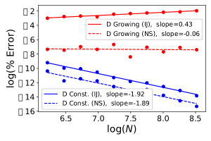
Figure 1: Log percent error (Eq. 10) of existing approximate LOOCV methods (“IJ” and “NS”) as a function of dataset size $N$ for $\ell_{2}$ regularized logistic regression. Dashed lines show Eq. 2 (“NS”) and solid show Eq. 3 (“IJ”). Blue lines have fixed data/parameter dimension $D$, while red lines have $D=N/10$, although the true parameter has a fixed support size of $D_{\mathrm{eff}}=2$ (see Section 2 for a full description). IJ and NS fail to capture this low “effective dimension” and suffer from substantially worse performance in high dimensions.

Model assessment vs. selection. Stone (1974); Geisser (1975) distinguish at least two uses of CV: model assessment and model selection. Model assessment refers to estimating the performance of a single, fixed model. Model selection refers to choosing among a collection of competing models. We focus almost entirely on model assessment – for two principal reasons. First, as discussed above, CV is widely used for model assessment in critical applied areas – such as medicine and genetics. Before we can safely apply approximate CV for model assessment in these areas, we need to empirically and theoretically verify our methods. Second, historically, rigorous analysis of the properties of model selection even for exact CV has required significant additional work beyond analyzing CV for model assessment. In fact, exact CV for model selection has only recently begun to be theoretically understood for $\ell_{1}$ regularized linear regression (Homrighausen and McDonald, 2013, 2014; Chetverikov et al., 2020). Our experiments in Appendix H confirm that approximate CV for model selection exhibits complex behavior. We thus expect significant further work, outside the scope of the present paper, to be necessary to develop a theoretical understanding of approximate CV for model selection. Indeed, to the best of our knowledge, all existing theory for the accuracy of approximate CV applies only to model assessment (Beirami et al., 2017; Rad and Maleki, 2020; Giordano et al., 2019b; Xu et al., 2019; Koh et al., 2019).

2 Overview of Approximations

Let $\theta\in\Theta\subseteq\mathbb{R}^{D}$ be an unknown parameter of interest. Consider a dataset of size $N$, where $n\in[N]:=\{1,2,\ldots,N\}$ indexes the data point. Then a number of problems – such as maximum likelihood, general M-estimation, and regularized loss minimization – can be expressed as solving

$$\hat{\theta}:=\operatorname*{arg\,min}_{\theta\in\Theta}\frac{1}{N}\sum_{n=1}^{N}f_{n}(\theta)+\lambda R(\theta),$$ (1)

where $\lambda\geq 0$ is a constant, and $R:\Theta\to\mathbb{R}_{+}$ and $f_{n}:\Theta\to\mathbb{R}$ are functions. For instance, $f_{n}$ might be the loss associated with the $n$th data point, $R$ the regularizer, and $\lambda$ the amount of regularization. Consider a dataset where the $n$th data point has covariates $x_{n}\in\mathbb{R}^{D}$ and response $y_{n}\in\mathbb{R}$. In what follows, we will be interested in taking advantage of sparsity. With this in mind, we focus on generalized linear models (GLMs), where $f_{n}(\theta)=f(x_{n}^{T}\theta,y_{n})$, as they offer a natural framework where sparsity can be expressed by choosing many parameter dimensions to be zero.

In LOOCV, we are interested in solutions of the same problem with the $n$th data point removed. To that end, define $\hat{\theta}_{\backslash n}:=\operatorname*{arg\,min}_{\theta\in\Theta}\frac{1}{N}\sum_{m:\,m\neq n}f_{m}(\theta)+\lambda R(\theta)$. Computing $\hat{\theta}_{\backslash n}$ exactly across $n$ usually requires $N$ runs of an optimization procedure – a prohibitive cost. Various approximations, detailed next, address this cost by solving Eq. 1 only once.

Two approximations. Assume that $f$ and $R$ are twice differentiable functions of $\theta$. Let $F(\theta):=(1/N)\sum_{n}f(x_{n}^{T}\theta,y_{n})$ be the unregularized objective, and let $H(\theta):=\nabla^{2}_{\theta}F(\theta)+\lambda\nabla^{2}_{\theta}R(\theta)$ be the Hessian matrix of the full objective. For the moment, we assume appropriate terms in each approximation below are invertible. Beirami et al. (2017); Rad and Maleki (2020); Wang et al. (2018); Koh et al. (2019) approximate $\hat{\theta}_{\backslash n}$ by taking a Newton step (“NS”) on the objective $(1/N)\sum_{m:\,m\neq n}f_{m}+\lambda R$ starting from $\hat{\theta}$; see Section D.4 for details. We thus call this approximation $\widetilde{\mathrm{NS}}_{\setminus n}(R)$ for regularizer $R$:

$$\widetilde{\mathrm{NS}}_{\setminus n}(R):=\hat{\theta}+\frac{1}{N}\left(H(\hat{\theta})-\frac{1}{N}\nabla^{2}_{\theta}f_{n}(\hat{\theta})\right)^{-1}\nabla_{\theta}f_{n}(\hat{\theta}).$$ (2)

In the case of GLMs, Theorem 8 of Rad and Maleki (2020) gives conditions on $x_{n}$ and $f(\cdot,\cdot)$ that imply, for fixed $D$, the error of $\widetilde{\mathrm{NS}}_{\setminus n}(R)$ averaged over $n$ is $o(1/N)$ as $N\to\infty$.

Koh and Liang (2017); Beirami et al. (2017); Giordano et al. (2019b); Koh et al. (2019) consider a second approximation. As their approximation is inspired by the infinitesimal jackknife (“IJ”) (Jaeckel, 1972; Efron, 1982), we denote it by $\widetilde{\mathrm{IJ}}_{\setminus n}(R)$; see Section D.1.

$$\widetilde{\mathrm{IJ}}_{\setminus n}(R):=\hat{\theta}+\frac{1}{N}H(\hat{\theta})^{-1}\nabla_{\theta}f_{n}(\hat{\theta}).$$ (3)

Giordano et al. (2019b) study the case of $\lambda=0$, and, in their Corollary 1, show that the accuracy of Eq. 3 is bounded by $C/N$ in general or, in the case of bounded gradients $\|\nabla_{\theta}f(x_{n}^{T}\theta,y_{n})\|_{\infty}\leq B$, by $C^{\prime}B/N^{2}$. The constants $C,C^{\prime}$ may depend on $D$ but not $N$. Our Proposition 2 in Section D.3 extends this result to the regularized case, $\lambda\geq 0$. Still, we are left with the fact that $C$ and $C^{\prime}$ depend on $D$ in an unknown way.

In what follows, we consider both $\widetilde{\mathrm{NS}}_{\setminus n}(R)$ and $\widetilde{\mathrm{IJ}}_{\setminus n}(R)$, as they have complimentary strengths. Empirically, we find that $\widetilde{\mathrm{NS}}_{\setminus n}(R)$ performs better in our LOOCV GLM experiments. But $\widetilde{\mathrm{IJ}}_{\setminus n}(R)$ is computationally efficient beyond LOOCV and GLMs. E.g., for general models, computation of $\widetilde{\mathrm{NS}}_{\setminus n}(R)$ requires inversion of a new Hessian for each $n$, whereas $\widetilde{\mathrm{IJ}}_{\setminus n}(R)$ needs only the inversion of $H(\hat{\theta})$ for all $n$. In terms of theory, $\widetilde{\mathrm{NS}}_{\setminus n}(R)$ has a tighter error bound of $o(1/N)$ for GLMs. But the theory behind $\widetilde{\mathrm{IJ}}_{\setminus n}(R)$ applies more generally, and, given a good bound on the gradients, may provide a tighter rate.

3 Problems in high dimensions

In the above discussion, we noted that there exists encouraging theory governing the behavior of $\widetilde{\mathrm{NS}}_{\setminus n}(R)$ and $\widetilde{\mathrm{IJ}}_{\setminus n}(R)$ when $D$ is fixed and $N$ grows large. We now describe issues with $\widetilde{\mathrm{NS}}_{\setminus n}(R)$ and $\widetilde{\mathrm{IJ}}_{\setminus n}(R)$ when $D$ is large relative to $N$. The first challenge for both approximations given large $D$ is computational. Since every variant of CV or approximate CV requires running the machine learning algorithm of interest at least once, we will focus on the cost of the approximations after this single run. Given $\hat{\theta}$, both approximations require the inversion of a $D\times D$ matrix. Calculation of $\widetilde{\mathrm{IJ}}_{\setminus n}(R)$ across $n\in[N]$ requires a single matrix inversion and $N$ matrix multiplications for a runtime in $O(D^{3}+ND^{2})$. In general, calculating $\widetilde{\mathrm{NS}}_{\setminus n}(R)$ has runtime of $O(ND^{3})$ due to needing an inversion for each $n$. In the case of GLMs, though, $\nabla^{2}_{\theta}f_{n}$ is a rank-one matrix, so standard rank-one updates give a runtime of $O(D^{3}+ND^{2})$ as well.

The second challenge for both approximations is the invertibility of $H(\hat{\theta})$ and $H(\hat{\theta})-(1/N)\nabla_{\theta}^{2}f(x_{n}^{T}\theta,y_{n})$ that was assumed in defining $\widetilde{\mathrm{NS}}_{\setminus n}(R)$ and $\widetilde{\mathrm{IJ}}_{\setminus n}(R)$. We note that, if $\nabla^{2}R(\hat{\theta})$ is only positive semidefinite, then invertibility of both matrices may be impossible when $D\geq N$; see Section D.2 for more discussion.

The third and final challenge for both approximations is accuracy in high dimensions. Not only do existing error bounds behave poorly (or not exist) in high dimensions, but empirical performance degrades as well. To create Fig. 1, we generated datasets from a sparse logistic regression model with $N$ ranging from 500 to 5,000. For the blue lines, we set $D=2$, and for the red lines we set $D=N/10$. In both cases, we see that error is much lower when $D$ is small and fixed.

We recall that for large $N$ and small $D$, training error often provides a fine estimate of the out-of-sample error (e.g., see (Vapnik, 1992)). That is, CV is needed precisely in the high-dimensional regime, and this case is exactly where current approximations struggle both computationally and statistically. Thus, we wish to understand whether there are high-$D$ cases where approximate CV is useful. In what follows, we consider a number of options for tackling one or more of these issues and show that only one method is effective in high dimensions.

Proposal #1: Use randomized solvers to reduce computation. Previously, Koh and Liang (2017) have utilized $\widetilde{\mathrm{IJ}}_{\setminus n}(R)$ for qualitative purposes, in which they are interested in its sign and relative magnitude across different $n$. They tackle the $O(D^{3})$ scaling of $\widetilde{\mathrm{IJ}}_{\setminus n}(R)$ by using the randomized solver from Agarwal et al. (2017). While one might hope to replicate the success of Koh and Liang (2017) in the context of approximate CV, we show in Appendix C that this randomized solver performs poorly for approximating CV: while it can be faster than exactly solving the needed linear systems, it provides an approximation to exact CV that can be an order of magnitude less accurate.

3.1 Sparsity via $\ell_{1}$ regularization.

Intuitively, if the exact $\hat{\theta}_{\backslash n}$’s have some low “effective dimension” $D_{\mathrm{eff}}\ll D$, we might expect approximate CV’s accuracy to depend only on $D_{\mathrm{eff}}$. One way to achieve low $D_{\mathrm{eff}}$ is sparsity: i.e., we have $\hat{D}_{\mathrm{eff}}:=\lvert\operatorname{supp}\hat{\theta}\rvert\ll D$, where $\hat{S}:=\operatorname{supp}\hat{\theta}$ collects the indices of the non-zero entries of $\hat{\theta}$. A way to achieve sparsity is choosing $R(\theta)=\|\theta\|_{1}$. However, note that $\widetilde{\mathrm{NS}}_{\setminus n}(R)$ and $\widetilde{\mathrm{IJ}}_{\setminus n}(R)$ cannot be applied directly in this case as $\|\theta\|_{1}$ is not twice-differentiable. Proposal #2: Rad and Maleki (2020); Wang et al. (2018) propose the use of a smoothed approximation to $\|\cdot\|_{1}$; however, as we show in Section 5, this approach is often multiple orders of magnitude more inaccurate and slower than Proposal #4 below.

Proposal #3: Subsample exact CV. Another option is to bypass all the problems of approximate CV in high-$D$ by uniformly subsampling a small collection of LOOCV folds. This provides an unbiased estimate of exact CV and can be used with exact $\ell_{1}$ regularization. However, our experiments (Section 5) show that, under a time budget, the results of this method are so variable that their error is often multiple orders of magnitude higher than Proposal #4 below.

Proposal #4: Use the sparsity from $\hat{\theta}$. Instead, in what follows, we take the intuitive approach of approximating CV only on the dimensions in $\operatorname{supp}\hat{\theta}$. Unlike all previously discussed options, we show that this approximation is fast and accurate in high dimensions in both theory and practice. For notation, let $X\in\mathbb{R}^{N\times D}$ be the covariate matrix, with rows $x_{n}$. For $S\subset[D]$, let $X_{\cdot,S}$ be the submatrix of $X$ with column indices in $S$; define $x_{nS}$ and $\theta_{S}$ similarly. Let $\hat{D}_{n}^{(2)}:=\left[d^{2}f(z,y_{n})/dz^{2}\right]_{z=x_{n}^{T}\hat{\theta}}$, and define the restricted Hessian evaluated at $\hat{\theta}$: $H_{\hat{S}\hat{S}}:=X_{\cdot,\hat{S}}^{T}\mathrm{diag}\{\hat{D}_{n}^{(2)}\}X_{\cdot,\hat{S}}$. Further define the LOO restricted Hessian, $H^{\backslash n}_{\hat{S}\hat{S}}:=H_{\hat{S}\hat{S}}-[\nabla^{2}_{\theta}f(x_{n}^{T}\hat{\theta},y_{n})]_{\hat{S}\hat{S}}$. Finally, without loss of generality, assume $\hat{S}=\{1,2,\dots,\hat{D}_{\mathrm{eff}}\}$. We now define versions of $\widetilde{\mathrm{NS}}_{\setminus n}(R)$ and $\widetilde{\mathrm{IJ}}_{\setminus n}(R)$ restricted to the entries in $\operatorname{supp}\hat{\theta}$:

$$\mathrm{NS}_{\backslash n}:=\begin{pmatrix}\hat{\theta}_{\hat{S}}+(H^{\backslash n}_{\hat{S}\hat{S}})^{-1}\left[\nabla_{\theta}f(x_{n}^{T}\hat{\theta},y_{n})\right]_{\hat{S}}\\ 0\end{pmatrix}$$ (4)

$$\mathrm{IJ}_{\backslash n}:=\begin{pmatrix}\hat{\theta}_{\hat{S}}+H_{\hat{S}\hat{S}}^{-1}\left[\nabla_{\theta}f(x_{n}^{T}\hat{\theta},y_{n})\right]_{\hat{S}}\\ 0\end{pmatrix}.$$ (5)

Other authors have previously considered $\mathrm{NS}_{\backslash n}$. Rad and Maleki (2020); Wang et al. (2018) derive $\mathrm{NS}_{\backslash n}$ by considering a smooth approximation to $\ell_{1}$ and then taking the limit of $\widetilde{\mathrm{NS}}_{\setminus n}(R)$ as the amount of smoothness goes to zero. In Appendix E, we show a similar argument can yield $\mathrm{IJ}_{\backslash n}$. Also, Obuchi and Kabashima (2016, 2018); Beirami et al. (2017) directly propose $\mathrm{NS}_{\backslash n}$ without using $\widetilde{\mathrm{NS}}_{\setminus n}(R)$ as a starting point. We now show how $\mathrm{NS}_{\backslash n}$ and $\mathrm{IJ}_{\backslash n}$ avoid the three major high-dimensional challenges with $\widetilde{\mathrm{NS}}_{\setminus n}(R)$ and $\widetilde{\mathrm{IJ}}_{\setminus n}(R)$ we discussed above.

The first challenge was that compute time for $\widetilde{\mathrm{NS}}_{\setminus n}(R)$ and $\widetilde{\mathrm{IJ}}_{\setminus n}(R)$ scaled poorly with $D$. That $\mathrm{NS}_{\backslash n}$ and $\mathrm{IJ}_{\backslash n}$ do not share this issue is immediate from their definitions.

Proposition 1.

For general $f_{n}$, the time to compute $\mathrm{NS}_{\backslash n}$ or $\mathrm{IJ}_{\backslash n}$ scales with $\hat{D}_{\mathrm{eff}}$, rather than $D$. In particular, computing $\mathrm{NS}_{\backslash n}$ across all $n\in[N]$ takes $O(N\hat{D}_{\mathrm{eff}}^{3})$ time, and computing $\mathrm{IJ}_{\backslash n}$ across all $n\in[N]$ takes $O(\hat{D}_{\mathrm{eff}}^{3}+N\hat{D}_{\mathrm{eff}}^{2})$ time. Furthermore, when $f_{n}$ takes the form of a GLM, computing $\mathrm{NS}_{\backslash n}$ across all $n\in[N]$ takes $O(\hat{D}_{\mathrm{eff}}^{3}+N\hat{D}_{\mathrm{eff}}^{2})$ time.

The second high-dimensional challenge was that $H$ and $H^{\setminus n}$ may not be invertible when $D\geq N$. Notice the relevant matrices in $\mathrm{NS}_{\backslash n}$ and $\mathrm{IJ}_{\backslash n}$ are of dimension $\hat{D}_{\mathrm{eff}}=\lvert\hat{S}\rvert$. So we need only make the much less restrictive assumption that $\hat{D}_{\mathrm{eff}}<N$, rather than $D<N$. We address the third and final challenge of accuracy in the next section.

4 Approximation quality in high dimensions

Recall that the accuracy of $\widetilde{\mathrm{NS}}_{\setminus n}(R)$ and $\widetilde{\mathrm{IJ}}_{\setminus n}(R)$ in general has a poor dependence on dimension $D$. We now show that the accuracy of $\mathrm{NS}_{\backslash n}$ and $\mathrm{IJ}_{\backslash n}$ depends on (the hopefully small) $\hat{D}_{\mathrm{eff}}$ rather than $D$. We start by assuming a “true” population parameter $\theta^{*}\in\mathbb{R}^{D}$ that minimizes the population-level loss, $\theta^{*}:=\operatorname*{arg\,min}\mathbb{E}_{x,y}[f(x^{T}\theta,y)]$, where the expectation is over $x,y$ from some population distribution. Assume $\theta^{*}$ is sparse with $S:=\operatorname{supp}\theta^{*}$ and $D_{\mathrm{eff}}:=|S|$. Our parameter estimate would be faster and more accurate if an oracle told us $S$ in advance and we worked just over $S$:

$$\hat{\phi}:=\operatorname*{arg\,min}_{\phi\in\mathbb{R}^{D_{\mathrm{eff}}}}\frac{1}{N}\sum_{n=1}^{N}f(x_{nS}^{T}\phi,y_{n})+\lambda\left\lVert\phi\right\rVert_{1}.$$ (6)

We define $\hat{\phi}_{\backslash n}$ as the leave-one-out variant of $\hat{\phi}$ (as $\hat{\theta}_{\backslash n}$ is to $\hat{\theta}$). Let $\mathrm{RNS}_{\backslash n}$ and $\mathrm{RIJ}_{\backslash n}$ be the result of applying the approximation in $\mathrm{NS}_{\backslash n}$ or $\mathrm{IJ}_{\backslash n}$ to the restricted problem in Eq. 6; note that $\mathrm{RNS}_{\backslash n}$ and $\mathrm{RIJ}_{\backslash n}$ have accuracy that scales with the (small) dimension $D_{\mathrm{eff}}$.

Our analysis of the accuracy of $\mathrm{NS}_{\backslash n}$ and $\mathrm{IJ}_{\backslash n}$ will depend on the idea that if, for all $n$, $\mathrm{NS}_{\backslash n}$, $\mathrm{IJ}_{\backslash n}$, and $\hat{\theta}_{\backslash n}$ run over the same $D_{\mathrm{eff}}$-dimensional subspace, then the accuracy of $\mathrm{NS}_{\backslash n}$ and $\mathrm{IJ}_{\backslash n}$ must be identical to that of $\mathrm{RNS}_{\backslash n}$ and $\mathrm{RIJ}_{\backslash n}$. In the case of $\ell_{1}$ regularization, this idea specializes to the following condition, under which our main result in Theorem 1 will be immediate.

Condition 1.

For all $n\in[N]$, we have $\operatorname{supp}\mathrm{IJ}_{\backslash n}=\operatorname{supp}\mathrm{NS}_{\backslash n}=\operatorname{supp}\hat{\theta}_{\backslash n}=S$.

Theorem 1.

Assume Condition 1 holds. Then for all $n$, $\hat{\theta}_{\backslash n}$ and $\mathrm{IJ}_{\backslash n}$ are (1) zero outside the dimensions $S$ and (2) equal to their restricted counterparts from Eq. 6:

$$\hat{\theta}_{\backslash n}=\begin{pmatrix}\hat{\theta}_{\backslash n,S}\\ 0\end{pmatrix}=\begin{pmatrix}\hat{\phi}_{\backslash n}\\ 0\end{pmatrix},\;\;$$

$$\mathrm{IJ}_{\backslash n}=\begin{pmatrix}\mathrm{IJ}_{\backslash n,S}\\ 0\end{pmatrix}=\begin{pmatrix}\mathrm{RIJ}_{\backslash n}\\ 0\end{pmatrix}.$$ (7)

It follows that the error is the same in the full problem as in the low-dimensional restricted problem: $\|\hat{\theta}_{\backslash n}-\mathrm{IJ}_{\backslash n}\|_{2}=\|\hat{\phi}_{\backslash n}-\mathrm{RIJ}_{\backslash n}\|_{2}$. The same results hold for $\mathrm{IJ}_{\backslash n}$ and $\mathrm{RIJ}_{\backslash n}$ replaced by $\mathrm{NS}_{\backslash n}$ and $\mathrm{RNS}_{\backslash n}$.

Taking Condition 1 as a given, Theorem 1 tells us that for $\ell_{1}$ regularized problems, $\mathrm{IJ}_{\backslash n}$ and $\mathrm{NS}_{\backslash n}$ inherit the fixed-dimensional accuracy of $\widetilde{\mathrm{IJ}}_{\setminus n}(R)$ and $\widetilde{\mathrm{NS}}_{\setminus n}(R)$ shown empirically in Fig. 1 and described theoretically in the references from Section 1. Taking a step further, one could show that $\mathrm{IJ}_{\backslash n}$ and $\mathrm{NS}_{\backslash n}$ are accurate for model assessment tasks by using results on the accuracy of exact CV for assessment (e.g., (Abou-Moustafa and Szepesvári, 2018; Steinberger and Leeb, 2018; Barber et al., 2019)).

Again, Theorem 1 is immediate if one is willing to assume Condition 1, but when does Condition 1 hold? There exist assumptions in the $\ell_{1}$ literature under which $\operatorname{supp}\hat{\theta}=S$ (Lee et al., 2014; Li et al., 2015). If one took these assumptions to hold for all $F^{\backslash n}:=(1/N)\sum_{m:\,m\neq n}f_{m}$, then Condition 1 would directly follow. However, it is not immediate that any models of interest meet such assumptions. Rather than taking such uninterpretable assumptions or just taking Condition 1 as an assumption directly, we will give a set of more interpretable assumptions under which Condition 1 holds.

In fact, we need just four principal assumptions in the case of linear and logistic regression; we conjecture that similar results hold for other GLMs. The first assumption arises from the intuition that, if individual data points are very extreme, the support will certainly change for some $n$. To avoid these extremes with high probability, we assume that the covariates follow a sub-Gaussian distribution:

Definition 1.

[e.g., Vershynin (2018)] For $c_{x}>0$, a random variable $V$ is $c_{x}$-sub-Gaussian if $\mathbb{E}\left[\exp\left(V^{2}/c_{x}^{2}\right)\right]\leq 2.$

Assumption 1.

Each $x_{n}\in\mathbb{R}^{D}$ has zero-mean i.i.d. $c_{x}$-sub-Gaussian entries with $\mathbb{E}[x_{nd}^{2}]=1$.

We conjecture that the unit-variance part of the assumption is unnecessary. Conditions on the distributions of the responses $y_{n}$ will be specific to linear and logistic regression and will be given in Assumptions 5 and 6, respectively. Our results below will hold with high probability under these distributions. Note there are reasons to expect we cannot do better than high-probability results. In particular, Xu et al. (2012) show that there exist worst-case training datasets for which sparsity-inducing methods like $\ell_{1}$ regularization are not stable as each datapoint is left out.

Our second principal assumption is an incoherence condition.

Assumption 2.

The incoherence condition holds with high probability over the full dataset:

$$\Pr\left[\left\lVert\nabla F(\theta^{*})_{S^{c},S}\left(\nabla^{2}F(\theta^{*})_{SS}\right)^{-1}\right\rVert_{\infty}<1-\alpha\right]\leq e^{-25},$$

Authors in the $\ell_{1}$ literature often assume that incoherence holds deterministically for a given design matrix $X$ – starting from the introduction of incoherence by Zhao and Yu (2006) and continuing in more recent work (Lee et al., 2014; Li et al., 2015). Similarly, we will take our high probability version in Assumption 2 as given. But we note that Assumption 2 is at least known to hold for the case of linear regression with an i.i.d. Gaussian design matrix (e.g., see Exercise 11.5 of Hastie et al. (2015)). We next place some restrictions on how quickly $D$ and $D_{\mathrm{eff}}$ grow as functions of $N$.

Assumption 3.

As functions of $N$, $D$ and $D_{\mathrm{eff}}$ satisfy: (1) $D=o(e^{N})$, (2) $D_{\mathrm{eff}}=o([N/\log N]^{2/5})$, and (3) $D_{\mathrm{eff}}^{3/2}\sqrt{\log D}=o(N)$.

The constraints on $D$ here are particularly loose. While those on $D_{\mathrm{eff}}$ are tighter, we still allow polynomial growth of $D_{\mathrm{eff}}$ in $N$ for some lower powers of $N$. Our final assumption is on the smallest entry of $\theta^{*}_{S}$. Such conditions – typically called beta-min conditions – are frequently used in the $\ell_{1}$ literature to ensure $\hat{S}=S$ (Wainwright, 2009; Lee et al., 2014; Li et al., 2015).

Assumption 4.

$\theta^{*}$ satisfies $\min_{s\in S}\lvert\theta^{*}_{s}\rvert>\sqrt{D_{\mathrm{eff}}}T_{min}\lambda,$ where $T_{min}$ is some constant relating to the objective function $f$; see Assumption 15 in Section I.1 for an exact description.

4.1 Linear regression

We now give the distributional assumption on the responses $y_{n}$ in the case of linear regression and then show that Condition 1 holds.

Assumption 5.

$\forall n,y_{n}=x_{n}^{T}\theta^{*}+\varepsilon_{n}$, where the $\varepsilon_{n}$ are i.i.d. $c_{\varepsilon}$-sub-Gaussian random variables.

Theorem 2 (Linear Regression).

Take Assumptions 1, 2, 4, 5 and 3. Suppose the regularization parameter $\lambda$ satisfies

$$\lambda\geq\frac{C}{\alpha-M_{\mathrm{lin}}} \left(\sqrt{\frac{c_{x}^{2}c_{\varepsilon}^{2}\log D}{N}+\frac{25c_{x}^{2}c_{\varepsilon}^{2}}{N}}\right.$$

$$\left.\quad+\frac{4c_{x}c_{\varepsilon}(\log(ND)+26)}{N}\right),$$ (8)

where $C>0$ is a constant in $N,D,D_{\mathrm{eff}},c_{x}$, and $c_{\varepsilon}$, and $M_{\mathrm{lin}}$ is a scalar given by Eq. 36 in Appendix I that satisfies, as $N\to\infty$, $M_{\mathrm{lin}}=o(1)$. Then for $N$ sufficiently large, Condition 1 holds with probability at least $1-26e^{-25}$.

A full statement and proof of Theorem 2, including the exact value of $M_{\mathrm{lin}}$, appears in Appendix I. A corollary of Theorem 1 and Theorem 2 together is that, under Assumptions 4, 1, 2, 3 and 5, the LOOCV approximations $\mathrm{IJ}_{\backslash n}$ and $\mathrm{NS}_{\backslash n}$ have accuracy that depends on (the ideally small) $D_{\mathrm{eff}}$ rather than (the potentially large) $D$.

It is worth considering how the allowed values of $\lambda$ in Eq. 8 compare to previous results in the $\ell_{1}$ literature for the support recovery of $\hat{\theta}$. We will talk about a sequence of choices of $\lambda$ scaling with $N$ denoted by $\lambda_{N}$. Theorem 11.3 of Hastie et al. (2015) shows that $\lambda_{N}\geq c\sqrt{\log(D)/N}$ (for some constant $c$ in $D$ and $N$) is sufficient for ensuring that $\operatorname{supp}\hat{\theta}\subseteq S$ with high probability in the case of linear regression. Thus, we ought to set $\lambda_{N}\geq c\sqrt{\log(D)/N}$ to ensure support recovery of $\hat{\theta}$. Compare this constraint on $\lambda_{N}$ to the constraint implied by Eq. 8. We have that $M_{\mathrm{lin}}=o(1)$ as $N\to\infty$, so that, for large $N$, the bound in Eq. 8 becomes $\lambda_{N}\geq c^{\prime}\sqrt{\log(D)/N}$ for some constant $c^{\prime}$. Thus, the sequence of $\lambda_{N}$ satisfying Eq. 8 scales at exactly the same rate as those that ensure $\operatorname{supp}\hat{\theta}\subseteq S$. The scaling of $\lambda_{N}$ is important, as the error in $\hat{\theta}$, $\|\hat{\theta}-\theta^{*}\|_{2}^{2}$, is typically proportional to $\lambda_{N}$. The fact that we have not increased the asymptotic scaling of $\lambda_{N}$ therefore means that we can enjoy the same decay of $\|\hat{\theta}-\theta^{*}\|_{2}^{2}$ while ensuring $\operatorname{supp}\hat{\theta}_{\backslash n}=S$ for all $n$.

4.2 Logistic regression

We now give the distributional assumption on the responses $y_{n}$ in the case of logistic regression.

Assumption 6.

$\forall n,$ we have $y_{n}\in\left\{\pm 1\right\}$ with $\Pr\left[y_{n}=1\right]=1/(1+e^{-x_{n}^{T}\theta^{*}})$.

We will also need a condition on the minimum eigenvalue of the Hessian.

Assumption 7.

Assume for some scalar $L_{min}$ that may depend on $N,D_{\mathrm{eff}},$ and $c_{x}$, we have

$$\Pr\left[\lambda_{min}\left(\nabla_{\theta}^{2}F(\theta^{*})_{SS}\right)\leq L_{min}\right]\leq e^{-25}.$$

Furthermore, assume the scaling of $L_{min}$ in $N$ and $D_{\mathrm{eff}}$ is such that, under Assumption 3 and for sufficiently large $N$, $L_{min}\geq CN$ for some constant $C$ that may depend on $c_{x}$.

In the case of linear regression, we did not need an analogue of Assumption 7, as standard matrix concentration results tell us that its Hessian satisfies Assumption 7 with $L_{min}=N-Cc_{x}^{2}\sqrt{ND_{\mathrm{eff}}}$ (see Lemma 2 in Appendix I). The Hessian for logistic regression is significantly more complicated, and it is typical in the $\ell_{1}$ literature to make some kind of assumption about its eigenvalues (Bach, 2010; Li et al., 2015). Empirically, Assumption 7 is satisfied when Assumptions 1 and 6 hold; however we are unaware of any results in the literature showing this is the case.

Theorem 3 (Logistic Regression).

Take Assumptions 1, 2, 4, 6, 3 and 7. Suppose the regularization parameter $\lambda$ satisfies:

$$\lambda\geq\frac{C}{\alpha-M_{\mathrm{logr}}} \left(\sqrt{c_{x}^{2}\frac{25+\log D}{N}}\right.$$

$$\quad\left.+\frac{\sqrt{2c_{x}^{2}\log(ND)}+\sqrt{50c_{x}^{2}}}{N}\right),$$ (9)

where $C,C^{\prime}$ are constants in $N,D,D_{\mathrm{eff}},$ and $c_{x}$, and $M_{\mathrm{logr}}$ is a scalar given by Eq. 67, that, as $N\to\infty$, satisfies $M_{\mathrm{logr}}=o(1)$. Then for $N$ sufficiently large, Condition 1 is satisfied with probability at least $1-43e^{-25}$.

A restatement and proof of Theorem 3 are given as Theorem 5 in Appendix I. Similar to the remarks after Theorem 2, Theorem 3 implies that when applied to logistic regression, $\mathrm{IJ}_{\backslash n}$ and $\mathrm{NS}_{\backslash n}$ have accuracy that depends on (the ideally small) $D_{\mathrm{eff}}$ rather than (the potentially large) $D$, even when $D=o(e^{N})$.

Theorem 3 has implications for the work of Obuchi and Kabashima (2018), who conjecture that, as $N\to\infty$, the change in support of $\ell_{1}$ regularized logistic regression becomes negligible as each datapoint is left out; this assumption is used to derive a version of $\mathrm{NS}_{\backslash n}$ for logistic regression. Our Theorem 3 confirms this conjecture by proving the stronger fact that the support is unchanged with high probability for finite data.

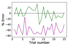
Figure 2: Error (Eq. 10) across approximations for $\ell_{1}$ LOOCV (legend shared with Fig. 3). The error for $\mathrm{IJ}_{\backslash n}$ (black dashed) is too small to see, but nonzero; it varies between $-0.06\%$ and $0.04\%$.

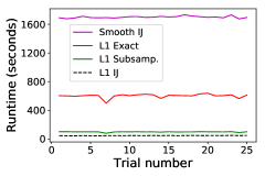
Figure 3: Runtimes for the experiments in Fig. 2 with exact CV (red) included for comparison. The $D\times D$ matrix inversion in the smoothed problem is so slow that even exact CV with an efficient $\ell_{1}$ solver is faster.

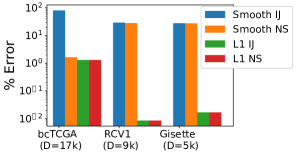
Figure 4: Log percent accuracy (Eq. 10) for real data experiments. For each dataset, we give the accuracy of approximate CV compared to exact CV using both a smoothed approximation to $\ell_{1}$ and the $\mathrm{IJ}_{\backslash n}$, $\mathrm{NS}_{\backslash n}$ approximations. For the bcTCGA dataset (linear regression), the nearly quadratic objective seems to be extremely well approximated by one Newton step, making $\widetilde{\mathrm{NS}}_{\setminus n}(R^{\eta})$ significantly more accurate than $\widetilde{\mathrm{IJ}}_{\setminus n}(R^{\eta})$; see the note at the end of Section D.4 about the exactness of $\widetilde{\mathrm{NS}}_{\setminus n}(R)$ on quadratic objectives.

5 Experiments

We now empirically verify the good behavior of $\mathrm{NS}_{\backslash n}$ and $\mathrm{IJ}_{\backslash n}$ (i.e. proposal #4) and show that it far outperforms #2 (smoothing $\ell_{1}$) and #3 (subsampling) in our high-dimensional regime of interest. All the code to run our experiments here is available online. We focus comparisons in this section on proposals #2–#4, as they all directly address $\ell_{1}$-regularized problems. For an illustration of the failings of proposal #1, see Appendix C. To illustrate #2, we consider the smooth approximation given by Rad and Maleki (2020): $R^{\eta}(\theta):=\sum_{d=1}^{D}\frac{1}{\eta}\big{(}\log(1+e^{\eta\theta_{d}})+\log(1+e^{-\eta\theta_{d}})\big{)}.$ While $\lim_{\eta\to\infty}R^{\eta}(\theta)=\left\lVert\theta\right\rVert_{1}$, we found that this approximation became numerically unstable for optimization when $\eta$ was much larger than 100, so we set $\eta=100$ in our experiments.

Simulated experiments. First, we trained logistic regression models on twenty-five random datasets in which $x_{nd}\overset{i.i.d.}{\sim}N(0,1)$ with $N=500$ and $D=40{,}000$. We set $\lambda=1.5\sqrt{\log(D)/N}$ to mimic our condition in Eq. 9. The true $\theta^{*}$ was supported on its first five entries. We evaluate our approximations by comparing the CV estimate of out-of-sample error (“$\mathrm{LOO}$”) to the approximation $\mathrm{ALOO}:=\frac{1}{N}\sum_{n=1}^{N}f(x_{n}^{T}\mathrm{IJ}_{\backslash n},y_{n}).$ We report percent error:

$$\lvert\mathrm{ALOO}-\mathrm{LOO}\rvert/\mathrm{LOO}.$$ (10)

Fig. 2 compares the accuracy and run times of proposals #2 and #3 versus $\mathrm{IJ}_{\backslash n}$. We chose the number of subsamples so that subsampling CV would have about the same runtime as computing $\mathrm{IJ}_{\backslash n}$ for all $n$. We see that subsampling usually has much worse accuracy than $\mathrm{IJ}_{\backslash n}$. Using $\widetilde{\mathrm{IJ}}_{\setminus n}(R)$ with $R^{100}(\theta)$ as a regularizer is even worse, as we approximate over all $D$ dimensions; the resulting approximation is slower and less accurate – by multiple orders of magnitude – across all trials.

The importance of setting $\lambda$.

Our theoretical results heavily depend on particular settings of $\lambda$ to obtain the fixed-dimensional error scaling shown in blue in Fig. 1. One might wonder if such a condition on $\lambda$ is necessary for approximate CV to be accurate. We offer evidence in Appendix F that this scaling is necessary by empirically showing that when $\lambda$ violates our condition, the error in $\mathrm{IJ}_{\backslash n}$ grows with $N$.

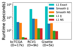
Figure 5: Log runtimes for experiments in Fig. 4, with exact CV included for comparison.

Real data experiments. We next study how dependent our results are on the particular distributional assumptions Theorems 2 and 3. We explore this question with a number of publicly available datasets (bcTCGA, 2018; Lewis et al., 2004; Guyon et al., 2004). We chose these datasets because they have a high enough dimension to observe the effect of our results, yet are not so large that running exact CV for comparison is prohibitively expensive; see Appendix G for details (including our settings of $\lambda$). For each dataset, we approximate CV for the $\ell_{1}$ regularized model using $\mathrm{IJ}_{\backslash n}$ and $\mathrm{NS}_{\backslash n}$. For comparison, we report the accuracy of $\widetilde{\mathrm{IJ}}_{\setminus n}(R^{\eta})$ and $\widetilde{\mathrm{NS}}_{\setminus n}(R^{\eta})$ with $\eta=100$. Our results in Fig. 4 show that $\mathrm{IJ}_{\backslash n}$ is significantly faster and more accurate than exact CV or smoothing.

To demonstrate the scalability of our approximations, we re-ran our RCV1 experiment on a larger version of the dataset with $N=20{,}242$ and $D=30{,}000$. Based on the time to compute exact LOOCV for twenty datapoints, we estimate exact LOOCV would have taken over two weeks to complete, whereas computing both $\mathrm{NS}_{\backslash n}$ and $\mathrm{IJ}_{\backslash n}$ for all $n$ took three minutes.

6 Conclusions and future work

We have provided the first analysis of when CV can be approximated quickly and accurately in high dimensions with guarantees on quality. We have seen that, out of a number of proposals in the literature, running approximate CV on the recovered support (i.e., $\mathrm{NS}_{\backslash n}$ and $\mathrm{IJ}_{\backslash n}$) forms the only proposal that reaches these goals both theoretically and empirically. We hope this analysis will serve as a starting point for further understanding of when approximate CV methods work for high-dimensional problems.

We see three interesting directions for future work. First, this work has focused entirely on approximate CV for model assessment. In Appendix H, we show that approximate CV for model selection can have unexpected and undesirable behavior; we believe understanding this behavior is one of the most important future directions in this area. Second, one could extend our results to results to the higher order infinitesimal jackknife presented in Giordano et al. (2019a). Finally, it would be interesting to consider our approximations as a starting point for subsampling estimators, as proposed in Magnusson et al. (2019).

Acknowledgements

This research is supported in part by DARPA, the CSAIL-MSR Trustworthy AI Initiative, an NSF CAREER Award, an ARO YIP Award, and ONR.

Appendix A Cross-validation methods

In this appendix, we review standard cross-validation (CV) for optimization problems of the form:

$$\operatorname*{arg\,min}_{\theta\in\Theta}\sum_{n=1}^{N}f_{n}(\theta)+\lambda R(\theta),$$

where $\Theta\subseteq\mathbb{R}^{D}$. By leave-one-out cross-validation (LOOCV), we mean the process of repeatedly computing:

$$\hat{\theta}_{\backslash n}:=\sum_{m:\,m\neq n}f_{m}(\theta)+\lambda R(\theta).$$

The parameter estimates $\{\hat{\theta}_{\backslash n}\}_{n=1}^{N}$ can then be used to produce an estimate of variability or out-of-sample error; e.g., to estimate the out-of-sample error, one computes $(1/N)\sum_{n}f_{n}(\hat{\theta}_{\backslash n})$. By $K$-fold cross-validation, we mean the process of splitting up the dataset into $K$ disjoint folds, $S_{1},\dots,S_{K}$ with $S_{1}\cup\dots\cup S_{K}=[N]$. One then estimates the parameters:

$$\hat{\theta}_{\backslash S_{k}}:=\operatorname*{arg\,min}_{\theta\in\Theta}\sum_{n:\,n\not\in S_{k}}f_{n}(\theta)+\lambda R(\theta).$$

The parameter estimates $\{\hat{\theta}_{\backslash S_{k}}\}_{k=1}^{K}$ can then be used to produce an estimate of variability or out-of-sample error.

Appendix B Scaling of the leave-one-out objective

We defined $\hat{\theta}_{\backslash n}$ as the solution to the following optimization problem:

$$\hat{\theta}_{\backslash n}:=\operatorname*{arg\,min}_{\theta\in\Theta}\frac{1}{N}\sum_{m:\,m\neq n}f_{m}(\theta)+\lambda R(\theta).$$

An alternative would be to use the objective $1/(N-1)\sum_{m:\,m\neq n}f_{m}+\lambda R$ in order to keep the scaling between the regularizer and the objective the same as in the full-data problem. Indeed, all existing theory that we are aware of for CV applied to $\ell_{1}$ regularized problems seems to follow the $1/(N-1)$ scaling [Homrighausen and McDonald, 2014, 2013, Miolane and Montanari, 2018, Chetverikov et al., 2020]. On the other hand, all existing approaches to approximate LOOCV for regularized problems have used the $1/N$ scaling that we have given [Beirami et al., 2017, Rad and Maleki, 2020, Wang et al., 2018, Xu et al., 2019, Obuchi and Kabashima, 2016, 2018]. Note that the scaling is not relevant in Giordano et al. [2019b], as they do not consider the regularized case. As our work is aimed at identifying when existing approximations work well in high dimensions, we have followed the $1/N$ choice from the literature on approximate LOOCV. The different results from using the two scalings may be insignificant when leaving only one datapoint out. But one might expect the difference to be substantial for, e.g., $K$-fold CV. We leave an understanding of what the effect of this scaling is (if any) to future work.

Appendix C Approximately solving $\widetilde{\mathrm{IJ}}_{\setminus n}(R)$ and $\widetilde{\mathrm{NS}}_{\setminus n}(R)$

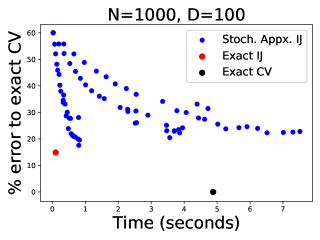
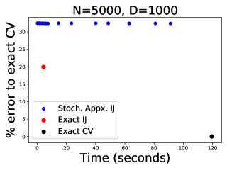
Figure 6: Stochastic Hessian experiments from Appendix C. We show percent error of approximation versus compute time for two different dataset sizes. We show three techniques for computing CV: exactly computing CV (black dot, which naturally has 0% error), $\widetilde{\mathrm{IJ}}_{\setminus n}(R)$ with exactly computing the needed linear systems (red dot), and $\widetilde{\mathrm{IJ}}_{\setminus n}(R)$ with the stochastic solves described in Appendix C (blue dots, one for each setting of the parameters $K$ and $M$). Values of $M$ and $K$ used are described in Appendix C; we use an extended range of settings for the smaller dataset to more extensively illustrate the approximation’s behavior. Settings of $K$ and $M$ for which the stochastic solves are roughly as fast as exactly computing $\widetilde{\mathrm{IJ}}_{\setminus n}(R)$ result in a significantly less accurate approximation of CV.

We have seen $\widetilde{\mathrm{IJ}}_{\setminus n}(R)$ and $\widetilde{\mathrm{NS}}_{\setminus n}(R)$ are in general not accurate for high-dimensional problems. Even worse, they can become prohibitively costly to compute due to the $O(D^{3})$ cost required to solve the needed linear systems. One idea to at least alleviate this computational burden, proposed by Koh and Liang [2017] in a slightly different context, is to use a stochastic inverse Hessian-vector-product from Agarwal et al. [2017] to approximately compute $\widetilde{\mathrm{IJ}}_{\setminus n}(R)$ and $\widetilde{\mathrm{NS}}_{\setminus n}(R)$. Although this method works well for the purposes of Koh and Liang [2017], we will see that in the context of approximate CV, it adds a large amount of extra error on top of the already inaccurate $\widetilde{\mathrm{NS}}_{\setminus n}(R)$ and $\widetilde{\mathrm{IJ}}_{\setminus n}(R)$.

We first describe this stochastic inverse Hessian-vector-product technique and argue that it is not suitable for approximating cross-validation. The main idea from Agarwal et al. [2017] is to use the series:

$$H^{-1}=\sum_{k=0}^{\infty}(I-H)^{k},$$

which holds for any positive definite $H$ with $\|H\|_{op}\leq 1$. Now, we can both truncate this series at some level $K$ and write it recursively as:

$$H^{-1}\approx H^{-1}_{K}:=I+(I-H)H^{-1}_{K-1},$$

where $H^{-1}_{0}=I$. Next, to avoid computing $H$ explicitly, we can note that if $A_{k}$ is some random variable with $E[A_{k}]=H$, we can instead just sample a new $A_{k}$ at each iteration to define:

$$\bar{H}^{-1}_{k}:=I+(I-A_{k})\bar{H}^{-1}_{K-1}.$$

In our case, we pick a random $n_{k}\in[N]$ and set $A_{k}=\nabla^{2}_{\theta}f(x_{n_{k}}^{T}\theta,y_{n_{k}})+(1/N)\lambda\nabla^{2}R(\theta)$. Finally, Agarwal et al. [2017] suggest taking $M$ samples of $\bar{H}^{-1}_{K}$ and averaging the results to lower the variance of the estimator. This leaves us with two parameters to tune: $M$ and $K$. Increasing either will make the estimate more accurate and more expensive to compute. Koh and Liang [2017] use this approximation to compute $\widetilde{\mathrm{IJ}}_{\setminus n}(R)$ for high dimensional models such as neural networks; however, we remark that their interest lies in the qualitative properties of $\widetilde{\mathrm{IJ}}_{\setminus n}(R)$, such as signs and relative magnitudes across various values of $n$. It remains to be seen whether this stochastic solver can be successfully used to approximate CV.

To test the application of this approximation to approximate CV, we generated a synthetic logistic regression dataset with covariates $x_{nd}\overset{i.i.d.}{\sim}N(0,1)$. We use $R(\theta)=\|\theta\|_{2}^{2}$. In Fig. 6, we show that for two settings of $N$ and $D$ there are no settings of $M$ and $K$ for which using $\bar{H}_{K}^{-1}$ to compute $\widetilde{\mathrm{IJ}}_{\setminus n}(R)$ provides a both fast and accurate approximation to CV. Specifically, we range $K\in\left\{1,20,30,50,60,80,100,120\right\}$ and $M\in\left\{2,25\right\}$ and see that when the stochastic approximation is faster, it provides only a marginal speedup while providing a significantly worse approximation error.

Appendix D Further details of Eq. 2 and Eq. 3

In Section 2, we briefly outlined the approximations $\widetilde{\mathrm{NS}}_{\setminus n}(R)$ and $\widetilde{\mathrm{IJ}}_{\setminus n}(R)$ to $\hat{\theta}_{\backslash n}$; we give more details about these approximations and their derivations here. Recall that we defined $H(\hat{\theta}):=(1/N)\sum_{n=1}^{N}\nabla_{\theta}^{2}f(x_{n}^{T}\hat{\theta},y_{n})+\lambda\nabla^{2}_{\theta}R(\hat{\theta})$. We first restate the “infinitesimal jackknife” approximation from the main text, which was derived by the same approach taken by Giordano et al. [2019b]:

$$\hat{\theta}_{\backslash n}\approx\widetilde{\mathrm{IJ}}_{\setminus n}(R):=\hat{\theta}+\frac{1}{N}H(\hat{\theta})^{-1}\nabla_{\theta}f(x_{n}^{T}\hat{\theta},y_{n}).$$ (11)

The “Newton step” approximation, similar to the approach in Beirami et al. [2017] and identical to the approximation in Rad and Maleki [2020], Wang et al. [2018], is:

$$\hat{\theta}_{\backslash n}\approx\widetilde{\mathrm{NS}}_{\setminus n}(R):=\hat{\theta}+\frac{1}{N}\bigg{(}H(\hat{\theta})-\frac{1}{N}\nabla^{2}_{\theta}f(x_{n}^{T}\hat{\theta},y_{n})\bigg{)}^{-1}\nabla_{\theta}f(x_{n}^{T}\hat{\theta},y_{n}).$$ (12)

D.1 Derivation of $\widetilde{\mathrm{IJ}}_{\setminus n}(R)$

We will see in Section D.3 that, after some creative algebra, $\widetilde{\mathrm{IJ}}_{\setminus n}(R)$ is an instance of $\hat{\theta}_{IJ}$ from Definition 2 of Giordano et al. [2019b]. However, this somewhat obscures the motivation for considering Eq. 11. As an alternative to jamming our problem setup into that considered by Giordano et al. [2019b], we can more directly obtain the approximation in Eq. 11 by a derivation only slightly different from that in Giordano et al. [2019b]. We begin by defining $\hat{\theta}^{w}$ as the solution to a weighted optimization problem with weights $w_{n}\in\mathbb{R}$:

$$\hat{\theta}^{w}:=\operatorname*{arg\,min}_{\theta\in\Theta}G(w,\theta):=\operatorname*{arg\,min}_{\theta\in\Theta}\frac{1}{N}\sum_{n=1}^{N}w_{n}f(x_{n}^{T}\theta,y_{n})+\lambda R(\theta),$$ (13)

where we assume $G$ to be twice continuously differentiable with an invertible Hessian at $\hat{\theta}^{\mathbf{1}}$ (where $\hat{\theta}^{\mathbf{1}}$ is the solution in Eq. 13 with all $w_{n}=1$). For example, we have that $\hat{\theta}_{\backslash n}=\hat{\theta}^{w}$ if $w$ is the $N$-dimensional vector of all ones but with a zero in the $n$th coordinate. We will form a linear approximation to $\hat{\theta}^{w}$ as a function of $w$. To do so, we will need to compute the derivatives $d\hat{\theta}^{w}/dw_{n}$ for each $n$. To compute these derivatives, we begin with the first order optimality condition of Eq. 13 and take a total derivative with respect to $w_{n}$:

$$\frac{\partial G}{\partial\theta}\Bigr{|}_{\begin{subarray}{c}w=1,\theta=\hat{\theta}^{\mathbf{1}}\end{subarray}}=0$$

$$\implies\frac{d}{dw_{n}}\frac{\partial G}{\partial\theta}\Bigr{|}_{\begin{subarray}{c}w=1,\theta=\hat{\theta}^{\mathbf{1}}\end{subarray}}=\frac{\partial^{2}G}{\partial\theta\partial w_{n}}\Bigr{|}_{\begin{subarray}{c}w=1,\theta=\hat{\theta}^{\mathbf{1}}\end{subarray}}\frac{dw_{n}}{dw_{n}}+\frac{\partial^{2}G}{\partial\theta^{2}}\Bigr{|}_{\begin{subarray}{c}w=1,\theta=\hat{\theta}^{\mathbf{1}}\end{subarray}}\frac{d\hat{\theta}^{w}}{dw_{n}}\Bigr{|}_{\begin{subarray}{c}w=1\end{subarray}}=0.$$

Re-arranging, defining $H(\hat{\theta}^{\mathbf{1}}):=\nabla^{2}_{\theta}G(w,\hat{\theta}^{\mathbf{1}})$, and using the assumed invertibility of $H(\hat{\theta}^{\mathbf{1}})$ gives:

$$\frac{d\hat{\theta}}{dw_{n}}\Bigr{|}_{\begin{subarray}{c}w=1\end{subarray}}=-\left(\frac{\partial^{2}G}{\partial\theta^{2}}\Bigr{|}_{\begin{subarray}{c}w=1,\theta=\hat{\theta}^{\mathbf{1}}\end{subarray}}\right)^{-1}\frac{\partial^{2}G}{\partial w_{n}\partial\theta}\Bigr{|}_{\begin{subarray}{c}w=1,\theta=\hat{\theta}^{\mathbf{1}}\end{subarray}}=-\frac{1}{N}H(\hat{\theta})^{-1}\nabla_{\theta}f(x_{n}^{T}\hat{\theta},y_{n}).$$ (14)

In the final equality, we used the fact that $\hat{\theta}^{\mathbf{1}}=\hat{\theta}$. Now, by a first order Taylor expansion around $w=(1,1,\dots,1)$, we can write:

$$\hat{\theta}^{w} \approx\hat{\theta}+\sum_{n=1}^{N}\frac{d\hat{\theta}}{dw_{n}}\Bigr{|}_{\begin{subarray}{c}w=1\end{subarray}}(w_{n}-1)$$ (15)

$$=\hat{\theta}-\frac{1}{N}\sum_{n=1}^{N}H(\hat{\theta})^{-1}\nabla_{\theta}f(x_{n}^{T}\hat{\theta},y_{n})(w_{n}-1).$$ (16)

For the special case of $w$ being the vector of all ones with a zero in the $n$th coordinate (i.e., the weighting for LOOCV), we recover Eq. 11.

D.2 Invertibility in the definition of $\widetilde{\mathrm{NS}}_{\setminus n}(R)$ and $\widetilde{\mathrm{IJ}}_{\setminus n}(R)$

In writing Eqs. 2 and 3 we have assumed the invertibility of $H(\hat{\theta})$ and $H(\hat{\theta})-(1/N)\nabla_{\theta}f(x_{n}^{T}\theta,y_{n})$. We here note a number of common cases where this invertibility holds. First, if $\nabla^{2}R$ is positive definite for all $\theta$ (as in the case of $R=\|\cdot\|_{2}^{2}$), then these matrices are always invertible. If $R$ is merely convex, $H(\hat{\theta})-(1/N)\nabla_{\theta}f(x_{n}^{T}\theta,y_{n})$ is invertible if $\mathrm{Span}\left\{x_{m}\right\}_{m:\,m\neq n}=\mathbb{R}^{D}$. This condition on the span holds almost surely if the $x_{n}$ are sampled from a continuous distribution and $D\leq N$.

D.3 Accuracy of $\widetilde{\mathrm{IJ}}_{\setminus n}(R)$ for regularized problems

As noted in the main text, Giordano et al. [2019b] show that the error of $\widetilde{\mathrm{IJ}}_{\setminus n}(R)$ is bounded by $C/N$ for some $C$ that is constant in $N$. However, their results apply only to the unregularized case (i.e., $\lambda=0$). We show here that their results can be extended to the case of $\lambda>0$ with mild additional assumptions; the proof of Proposition 2 appears below.

Proposition 2.

Assume that the conditions for Corollary 1 of Giordano et al. [2019b] are satisfied by $F(\theta)$. Furthermore, assume that we are restricted to $\theta$ in some compact subset $\Theta$ of $\mathbb{R}^{D}$, $\lambda=O(1/\sqrt{N})$, $F+\lambda R$ is twice continuously differentiable for all $\theta$, and that $\nabla^{2}R(\theta)$ is positive definite for all $\theta\in\Theta$. Then $\widetilde{\mathrm{IJ}}_{\setminus n}(R)$ can be seen as an application of the approximation in Definition 2 of Giordano et al. [2019b]. Furthermore, the assumptions of their Corollary 1 are met, which implies:

$$\max_{n\in[N]}\|\tilde{\psi}^{\backslash n}_{IJ}-\hat{\theta}_{\backslash n}\|_{2}\leq\frac{C^{\prime}}{N^{2}}\sup_{\theta\in\Theta}\max_{n\in[N]}\left\lVert\nabla_{\theta}f(x_{n}^{T}\theta,y_{n})\right\rVert_{\infty}\leq\frac{C}{N},$$ (17)

where $C$ and $C^{\prime}$ are problem-specific constants independent of $N$ that may depend on $D$.

Proposition 2 provides two bounds on the error $\|\widetilde{\mathrm{IJ}}_{\setminus n}(R)-\hat{\theta}_{\backslash n}\|_{2}$: either $C^{\prime}/N^{2}$ times the maximum of the gradient or just $C/N$. One bound or the other may be easier to use, depending on the specific problem. It is worth discussing the conditions of Proposition 2 before going into its proof. The first major assumption is that $\theta$ is restricted to some compact set $\Theta$. Although this assumption may not be satisfied by problems of interest, one may be willing to assume that $\theta$ lives in some bounded set in practice. In any case, such an assumption seems necessary to apply the results of Giordano et al. [2019b] to most unregularized problems, as they, for example, require $\sup_{\theta\in\Theta}F(\theta)$ to be bounded. We will require the compactness of $\Theta$ to show that $\sup_{\theta\in\Theta}F(\theta)+\lambda R(\theta)$ is bounded.

The second major assumption of Proposition 2 is that $\lambda=O(1/\sqrt{N})$. We need this assumption to ensure that the term $\lambda R(\theta)$ is sufficiently well behaved. In practice this assumption may be somewhat limiting; however, we note that for fixed D, such a scaling is usually assumed – and in some situations is necessary – to obtain standard theoretical results for $\ell_{1}$ regularization (e.g., Wainwright [2009] gives the standard scaling for linear regression, $\lambda=\Omega(\sqrt{\log(D)/N})$). Our Theorems 2 and 3 also satisfy such a scaling when D is fixed. In any case, we stress that this assumption – as well as the assumption on compactness – are needed only to prove Proposition 2, and not any of our other results. We prove Proposition 2 to demonstrate the baseline results that exist in the literature so that we can then show how our results build on these baselines.

Proof.

We proceed by showing that the regularized optimization problem in our Eq. 1 can be written in the framework of Eq. (1) of Giordano et al. [2019b] and then showing that the re-written problem satisfies the assumptions of their Corollary 1. First, the framework of Giordano et al. [2019b] applies to weighted optimization problems of the form:

$$\hat{\theta}^{w}:=\theta\in\Theta\;s.t.\;\frac{1}{N}\sum_{n=1}^{N}w_{n}g_{n}(\theta)=0.$$ (18)

In order to match this form, we will rewrite the gradient of the objective in Eq. 1 as a weighted sum with $N+1$ terms, where the first term, with weight $w_{0}=1$, will correspond to $R(\theta)$:

$$\frac{1}{N+1}w_{0}(N+1)\lambda\nabla R(\theta)+\frac{1}{N+1}\sum_{n=1}^{N}w_{n}\frac{N+1}{N}\nabla f(x_{n}^{T}\theta,y_{n}).$$ (19)

We will also need a set of weight vectors $W\subseteq\mathbb{R}^{N+1}$ for which we are interested in evaluating $\hat{\theta}^{w}$. We choose this set as follows. In the set, we include each weight vector that is equal to one everywhere except $w_{n}=0$ for exactly one of $n\in\{1,\ldots,N\}$. Thus, for each $n$, there is a $w\in W$ such that $\hat{\theta}^{w}=\hat{\theta}_{\backslash n}$. Finally, then, we can apply Definition 2 of Giordano et al. [2019b] to find the approximation $\theta_{IJ}(w)$ for the $w$ that corresponds to leaving out $n$. We see that $\theta_{IJ}(w)$ in this case is exactly equal to $\widetilde{\mathrm{IJ}}_{\setminus n}(R)$ in our notation here.

Now that we know our approximation is actually an instance of $\theta_{IJ}(w)$, we need to check that Eq. 19 meets the assumptions of Corollary 1 of Giordano et al. [2019b] to apply their theoretical analysis to our problem. We check these below, first stating the assumption from Giordano et al. [2019b] and then covering why it holds for our problem.

1. (Assumption 1): for all $\theta\in\Theta$, each $g_{n}$ is continuously differentiable in $\theta$.
   For our problem, by assumption, $R(\theta)$ and $f(x_{n}^{T}\theta,y_{n})$ are twice continuously differentiable functions of $\theta$, so this assumption holds.

2. (Assumption 2): for all $\theta\in\Theta$, the Hessian matrix, $H(\theta,1):=(1/N)\sum_{n}\partial g_{n}(\theta)/\partial\theta^{T}$ is invertible and satisfies $\sup_{\theta\in\Theta}\|H^{-1}(\theta,1)\|_{op}\leq C_{op}<\infty$ for some constant $C_{op}$, where $\|\cdot\|_{op}$ denotes the operator norm on matrices with respect to the $\ell_{2}$ norm (i.e., the maximum eigenvalue of the matrix).
   For our problem, by assumption, the inverse matrix $(\nabla^{2}F(\theta))^{-1}$ exists and has bounded maximum eigenvalue for all $\theta\in\Theta$. Also by assumption, $R$ has a positive semidefinite Hessian for all $\theta$, which implies:

   $$\sup_{\theta\in\Theta}\left\lVert H^{-1}(\theta,1)\right\rVert_{op}=\sup_{\theta\in\Theta}\left\lVert\left(\nabla^{2}F(\theta)+\lambda\nabla^{2}R(\theta)\right)^{-1}\right\rVert_{op}\leq\sup_{\theta\in\Theta}\left\lVert\left(\nabla^{2}F(\theta)\right)^{-1}\right\rVert_{op}.$$

   To see that the inequality holds, first note that for a positive semi-definite (PSD) matrix $A$, $\|A^{-1}\|_{op}=1/\lambda_{min}(A)$. The inequality would then follow if $\lambda_{min}(\nabla^{2}F(\theta)+\lambda\nabla^{2}R(\theta))\geq\lambda_{min}(\nabla^{2}F(\theta))$. To see that this holds, take any two $D\times D$ PSD matrices $A$ and $B$. Let $\lambda_{d}(\cdot)$ be the $d$th eigenvalue of a matrix with $\lambda_{1}=\lambda_{min}$. Then:

   $$\lambda_{d}(A+B)=\min_{\begin{subarray}{c}E\subseteq\mathbb{R}^{D}\\ \dim{E}=d\end{subarray}}\max_{\begin{subarray}{c}x\in E\\ \left\lVert x\right\rVert_{2}=1\end{subarray}}x^{T}(A+B)x\geq\min_{\begin{subarray}{c}E\subseteq\mathbb{R}^{D}\\ \dim{E}=d\end{subarray}}\max_{\begin{subarray}{c}x\in E\\ \left\lVert x\right\rVert_{2}=1\end{subarray}}x^{T}Ax=\lambda_{d}(A),$$

   where the inequality holds because $B$ is PSD. So, $\lambda_{min}(A+B)\geq\lambda_{min}(A)$, which finishes the proof. We have thus showed that the operator norm of $H^{-1}(\theta,1)$ is bounded by that of $\nabla^{2}F(\theta)^{-1}$ for all $\theta\in\Theta$.

3. (Assumption 3): Let $g(\theta)$ and $h(\theta)$ be the $(N+1)\times D$ stack of gradients and $(N+1)\times D\times D$ stack of Hessians, respectively. That is, $g(\theta)_{nd}:=(\nabla_{\theta}f(x_{n}^{T}\theta,y_{n}))_{d}$ for $n=1,\dots,N$ and $g(\theta)_{N+1,d}:=(\nabla_{\theta}R(\theta))_{d}$, with $h$ defined similarly. Let $\left\lVert g(\theta)\right\rVert_{2}$ be the $\ell_{2}$ norm of $g$ flattened into a vector with $\left\lVert h(\theta)\right\rVert_{2}$ defined similarly. Then assume that there exist constants $C_{g}$ and $C_{h}$ such that:

   $$\sup_{\theta\in\Theta}\frac{1}{\sqrt{N+1}}\left\lVert g(\theta)\right\rVert_{2}\leq C_{g}<\infty$$

   $$\sup_{\theta\in\Theta}\frac{1}{\sqrt{N+1}}\left\lVert h(\theta)\right\rVert_{2}\leq C_{h}<\infty$$

   To see that this holds for our problem, we have that:

   $$\left\lVert g(\theta)\right\rVert_{2} :=\left[\sum_{d=1}^{D}\left((\lambda(N+1)\nabla R(\theta)_{d})^{2}+\sum_{n=1}^{N}\left(\frac{N+1}{N}\right)^{2}(\nabla f(x_{n}^{T}\theta,y_{n})_{d})^{2}\right)\right]^{1/2}$$

   $$\leq\lambda(N+1)\left\lVert\nabla R(\theta)\right\rVert_{2}+\frac{N+1}{N}\left[\sum_{d=1}^{D}\sum_{n=1}^{N}(\nabla f(x_{n}^{T}\theta,y_{n})_{d})^{2}\right]^{1/2}.$$

   We need to show this is bounded by $\sqrt{N+1}C_{g}$ for some constant $C_{g}$. By assumption in the statement of Proposition 2, we have $\frac{1}{\sqrt{N+1}}\left\lVert\nabla F(\theta)\right\rVert_{2}\leq\frac{1}{\sqrt{N}}\left\lVert\nabla F(\theta)\right\rVert_{2}\leq C_{g}^{(1)}$ for some constant $C_{g}^{(1)}$. Because $\lambda$ is $O(1/\sqrt{N})$, the first term is equal to $O(\sqrt{N})\|\nabla R(\theta)\|_{2}$. The compactness of $\Theta$ and the continuity of $\nabla R(\theta)$ imply that $\|\nabla R(\theta)\|_{2}$ is bounded by a constant for all $\theta\in\Theta$. So, we know that $\frac{O(\sqrt{N})}{\sqrt{N+1}}\|\nabla R(\theta)\|_{2}\leq C_{g}^{(2)}$ for some constant $C_{g}^{(2)}$. Thus, we have that the assumption on $\|g(\theta)\|_{2}$ holds with $C_{g}=\frac{(N+1)}{N}C_{g}^{(1)}+C_{g}^{(2)}$. That the condition on $\|h(\theta)\|_{2}$ holds follows by the same reasoning.

4. (Assumption 4): There exists some $\Delta_{\theta}>0$ and $L_{h}<\infty$ such that if $\left\lVert\theta-\hat{\theta}\right\rVert_{2}\leq\Delta_{\theta}$, then $\frac{1}{\sqrt{N+1}}\left\lVert h(\theta)-h(\hat{\theta})\right\rVert_{2}\leq L_{h}\left\lVert\theta-\hat{\theta}\right\rVert_{2}$.
   We can show this holds for our problem by:

   $$\left\lVert h(\theta)-h(\hat{\theta})\right\rVert_{2} :=$$

   $$\left\lVert\frac{N+1}{N}\nabla^{2}F(\theta)+\lambda(N+1)\nabla^{2}R(\theta)-\frac{N+1}{N}\nabla^{2}F(\hat{\theta})-\lambda(N+1)\nabla^{2}R(\hat{\theta})\right\rVert_{2}$$

   $$\leq(N+1)\lambda\left\lVert\nabla^{2}R(\theta)-\nabla^{2}R(\hat{\theta})\right\rVert_{2}+\frac{N+1}{N}\left\lVert\nabla^{2}F(\theta)-\nabla^{2}F(\hat{\theta})\right\rVert_{2},$$

   where we have abused notation to denote $\left\lVert\nabla^{2}F(\theta)\right\rVert_{2}:=\sqrt{\sum_{i,j=1}^{D}\sum_{n=1}^{N}\nabla^{2}_{\theta}(f(x_{n}^{T}\theta,y_{n})_{ij})^{2}}$. Now, we want to show that this quantity divided by $\sqrt{N+1}$ is bounded by $L_{h}\|\theta-\hat{\theta}\|_{2}$ for some constant $L_{h}$. By assumption in the statement of Proposition 2, we have that Assumption 4 holds for $F$; this implies that $\frac{N+1}{(\sqrt{N+1})(N)}\left\lVert\nabla^{2}F(\theta)-\nabla^{2}F(\hat{\theta})\right\rVert_{2}\leq L_{h}^{(1)}\|\theta-\hat{\theta}\|_{2}$ for some constant $L_{h}^{(1)}$. As $R$ is twice continuously differentiable and the condition of Assumption 4 needs only to hold over a compact set of $\theta$’s, we know that $\nabla^{2}R(\theta)$ is Lipschitz over this domain. Using this along with the assumption that $\lambda$ is $O(1/\sqrt{N})$, we have that:

   $$\frac{\lambda(N+1)}{\sqrt{N+1}}\left\lVert\nabla^{2}R(\theta)-\nabla^{2}R(\hat{\theta})\right\rVert_{2} =O(1)\left\lVert\nabla^{2}R(\theta)-\nabla^{2}R(\hat{\theta})\right\rVert_{2}$$

   $$\leq L_{h}^{(2)}\left\lVert\theta-\hat{\theta}\right\rVert_{2},$$

   for some constant $L_{h}^{(2)}$. So, Assumption 4 holds with constant $L_{h}=L_{h}^{(1)}+L_{h}^{(2)}$.

5. (Assumption 5): For all $w\in W$, we have $\frac{1}{\sqrt{N+1}}\left\lVert w\right\rVert_{2}\leq C_{w}$ for some constant $C_{w}$. This is immediately true for our definition of $W$, which, for all $w\in W$, has $\|w\|_{2}=\sqrt{N}$.

∎

D.4 Derivation of $\widetilde{\mathrm{NS}}_{\setminus n}(R)$

Wang et al. [2018] and Rad and Maleki [2020] derive $\widetilde{\mathrm{NS}}_{\setminus n}(R)$ in Eq. 12 by taking a single Newton step on the objective $F^{\backslash n}+\lambda R$ starting at the point $\hat{\theta}$. For completeness, we include a derivation here. Recall that the objective with one datapoint left out is:

$$F^{\backslash n}(\theta)+\lambda R(\theta):=\frac{1}{N}\sum_{m=1}^{N}f(x_{m}^{T}\theta,y_{m})-\frac{1}{N}f(x_{n}^{T}\theta,y_{n})+\lambda R(\theta),$$ (20)

which has $H(\theta)-(1/N)\nabla_{\theta}^{2}f(x_{n}^{T}\theta,y_{n})$ as its Hessian. Now consider approximating $\hat{\theta}_{\backslash n}$ by performing a single Newton step on $F^{\backslash n}$ starting from $\hat{\theta}$:

$$\hat{\theta}_{\backslash n}\approx\hat{\theta}-\left(H(\hat{\theta})-\frac{1}{N}\nabla_{\theta}^{2}f(x_{n}^{T}\hat{\theta},y_{n})\right)^{-1}\left(\frac{1}{N}\sum_{m=1}^{N}\nabla_{\theta}f(x_{m}^{T}\hat{\theta},y_{m})-\frac{1}{N}\nabla_{\theta}f(x_{n}^{T}\hat{\theta},y_{n})+\lambda\nabla R(\hat{\theta})\right).$$ (21)

Using the fact that, by definition of $\hat{\theta}$, $(1/N)\sum_{n=1}^{N}\nabla_{\theta}f(x_{n}^{T}\hat{\theta},y_{n})+\lambda\nabla R(\hat{\theta})=0$, we have that this simplifies to:

$$\hat{\theta}_{\backslash n}\approx\hat{\theta}+\frac{1}{N}\left(H(\hat{\theta})-\frac{1}{N}\nabla_{\theta}^{2}f(x_{n}^{T}\hat{\theta},y_{n})\right)^{-1}\nabla_{\theta}f(x_{n}^{T}\hat{\theta},y_{n}),$$ (22)

which is exactly $\widetilde{\mathrm{NS}}_{\setminus n}(R)$.

As $\widetilde{\mathrm{NS}}_{\setminus n}(R)$ can be interpreted as a single Newton step on the objective $F^{\backslash n}+\lambda R$, it follows that $\widetilde{\mathrm{NS}}_{\setminus n}(R)$ is exactly equal to $\hat{\theta}_{\backslash n}$ in the case that $F^{\backslash n}+\lambda R$ is a quadratic, as noted by Beirami et al. [2017]. For example, $\ell_{2}$ regularized linear regression has $\widetilde{\mathrm{NS}}_{\setminus n}(R)=\hat{\theta}_{\backslash n}$ for all $n$. We further note that somewhat similar behavior can hold for $\ell_{1}$ regularized linear regression. Specifically, when $\mathrm{sign}\hat{\theta}=\mathrm{sign}\hat{\theta}_{\backslash n}$, we have that the objective $F^{\backslash n}+\lambda\left\lVert\cdot\right\rVert_{1}$ is a quadratic when restricted to the dimensions in $\hat{S}$. In this case, $\mathrm{NS}_{\backslash n}$ can be interpreted as taking a Newton step on $F^{\backslash n}+\lambda\left\lVert\cdot\right\rVert_{1}$ restricted to the dimensions in $\hat{S}$. It follows that $\mathrm{NS}_{\backslash n}=\hat{\theta}_{\backslash n}$ when $\mathrm{sign}\hat{\theta}=\mathrm{sign}\hat{\theta}_{\backslash n}$ for $\ell_{1}$ regularized linear regression.

D.5 Computation time of approximations

There is a major computational difference between Eq. 12 and Eq. 11: the former requires the inversion of a $D\times D$ matrix for each $\hat{\theta}_{\backslash n}$ approximated, while the latter requires a single $D\times D$ matrix inversion for all $\hat{\theta}_{\backslash n}$ inverted, which incurs a cost of $O(ND^{3})$ versus a cost of $O(D^{3})$. Even for small $D$, this is a significant additional expense.

However, as noted by Rad and Maleki [2020], Wang et al. [2018], Eq. 12 is much cheaper when considering the special case of generalized linear models. In this case, $\nabla_{\theta}^{2}f_{n}$ is some scalar times $x_{n}x_{n}^{T}$ – a rank one matrix. The Sherman-Morrison formula then allows us to cheaply compute the needed inverse in Eq. 12 given only $H^{-1}$; this is how Equation 8 in Rad and Maleki [2020] and Equation 21 in Wang et al. [2018] are derived. Even though we only consider GLMs in this work, we still study Eq. 11 with the hope of retaining scalability in more general problems.

Appendix E Derivation of $\mathrm{IJ}_{\backslash n}$ and $\mathrm{NS}_{\backslash n}$ via smoothed approximations

As noted in Section 2, Rad and Maleki [2020], Wang et al. [2018] derive the $\mathrm{NS}_{\backslash n}$ approximation by considering $\widetilde{\mathrm{NS}}_{\setminus n}(R^{\eta})$ with $R^{\eta}$ being some smoothed approximation to the $\ell_{1}$ norm, and then taking the limit of $\widetilde{\mathrm{NS}}_{\setminus n}(R^{\eta})$ as the amount of smoothness goes to zero. We review this approach and then state our Proposition 4, which says that the same technique can be used to derive $\mathrm{IJ}_{\backslash n}$.

We first give two possible ways to smooth the $\ell_{1}$ norm. The first is given by Rad and Maleki [2020]:

$$\left\lVert\theta\right\rVert_{1}\approx R^{\eta}(\theta):=\sum_{d=1}^{D}\frac{1}{\eta}\bigg{(}\log(1+e^{\eta\theta_{d}})+\log(1+e^{-\eta\theta_{d}})\bigg{)},$$ (23)

The second option is to use the more general smoothing framework described by Wang et al. [2018]. They allow selection of a function $q:\mathbb{R}\to\mathbb{R}$ satisfying: (1) $q$ has compact support, (2) $\int q(u)\;du=1$, $q(0)>0$, and $q\geq 0$, and (3) $q$ is symmetric around 0 and twice continuously differentiable on its domain, and then define a smoothed approximation:

$$R^{\eta}(\theta):=\eta\sum_{d=1}^{D}\int_{-\infty}^{\infty}\lvert u\rvert q\big{(}\eta(\theta_{d}-u)\big{)}du,$$ (24)

In both Eqs. 23 and 24, we have $\lim_{\eta\to\infty}=\|\theta\|_{1}$. Notice that either choice of $R^{\eta}$ is twice differentiable for any $\eta<\infty$, so one can consider the approximations $\widetilde{\mathrm{NS}}_{\setminus n}(R^{\eta}),\widetilde{\mathrm{IJ}}_{\setminus n}(R^{\eta})$. We now state two assumptions, both of which are given by Rad and Maleki [2020], Wang et al. [2018], under which one can show the limits of these approximations as $\eta\to\infty$ are equal to $\mathrm{NS}_{\backslash n}$ and $\mathrm{IJ}_{\backslash n}$.

Assumption 8.

For any element $\hat{z}\in\mathbb{R}^{D}$ of the subdifferential $\partial\left\lVert\theta\right\rVert_{1}$ evaluated at $\hat{\theta}$ such that $\nabla F(\hat{\theta})+\lambda\hat{z}=0$, we have $\left\lVert\hat{z}_{\hat{S}^{c}}\right\rVert_{\infty}<1$.

Assumption 9.

For any $y_{n}\in\mathbb{R}$, $f(z,y_{n})$ is a twice continuously differentiable function as a function of $z\in\mathbb{R}$.

Proposition 3 (Theorem 1 of Rad and Maleki [2020]; Theorem 4.2 of Wang et al. [2018]).

Take Assumptions 8 and 9. Suppose $H_{\hat{S}\hat{S}}$ has strictly positive eigenvalues. Let $H^{\backslash n}_{\hat{S}\hat{S}}:=H_{\hat{S}\hat{S}}-[\nabla^{2}_{\theta}f(x_{n}^{T}\hat{\theta},y_{n})]_{\hat{S}\hat{S}}$, and suppose that, for all $n$, $H^{\backslash n}_{\hat{S}\hat{S}}$ is invertible. Then, for $R^{\eta}$ as in Eq. 23 or Eq. 24,

$$\mathrm{NS}_{\backslash n}:=\lim_{\eta\to\infty}\widetilde{\mathrm{NS}}_{\setminus n}(R^{\eta})=\begin{pmatrix}\hat{\theta}_{\hat{S}}+(H^{\backslash n}_{\hat{S}\hat{S}})^{-1}\left[\nabla_{\theta}f(x_{n}^{T}\hat{\theta},y_{n})\right]_{\hat{S}}\\ \end{pmatrix}.$$ (25)

As noted in the main text, we show that a very similar result holds for the limit of $\widetilde{\mathrm{IJ}}_{\setminus n}(R^{\eta})$:

Proposition 4.

Take Assumptions 8 and 9. Suppose $H_{\hat{S}\hat{S}}$ is invertible. Then for $R^{\eta}$ as in Eq. 23 or Eq. 24:

$$\mathrm{IJ}_{\backslash n}:=\lim_{\eta\to\infty}\widetilde{\mathrm{IJ}}_{\setminus n}(R^{\eta})=\begin{pmatrix}\hat{\theta}_{\hat{S}}+H_{\hat{S}\hat{S}}^{-1}\left[\nabla_{\theta}f(x_{n}^{T}\hat{\theta},y_{n})\right]_{\hat{S}}\\ 0\end{pmatrix}.$$ (26)

The proof of Proposition 4 is a straightforward adaptation of the proof of Proposition 3. We prove it separately for the two different forms of $R^{\eta}$ in the next two subsections.

E.1 Proof of Proposition 4 using Eq. 23

This proof is almost identical to the proof of Theorem 1 from Rad and Maleki [2020]. First we will need some notation. Let $\hat{\theta}^{\eta}$ be the solution to Eq. 1 using $R^{\eta}$ from Eq. 23 as the regularizer. Let $\hat{S}_{\eta}:=\left\{i\;:\;\lvert\hat{\theta}^{\eta}\rvert>c/\eta\right\}$ for some constant $c$. We know from the arguments in Appendix A.2 of Rad and Maleki [2020] that for an appropriately chosen $c$ and $\eta>C$ for some large constant $C>0$, we have $S^{\eta}=\hat{S}=:\operatorname{supp}\hat{\theta}$. Next, define the scalars $\hat{D}_{n}^{(1,\eta)}$ and $\hat{D}_{n}^{(2,\eta)}$ as the derivatives of $f$ evaluated at $\hat{\theta}^{\eta}$:

$$\hat{D}_{n}^{(1,\eta)}:=\frac{df(z,y_{n})}{dz}\Bigr{|}_{\begin{subarray}{c}z=x_{n}^{T}\hat{\theta}^{\eta}\end{subarray}}\;,\quad\hat{D}_{n}^{(2,\eta)}:=\frac{d^{2}f(z,y_{n})}{dz^{2}}\Bigr{|}_{\begin{subarray}{c}z=x_{n}^{T}\hat{\theta}^{\eta}\end{subarray}}.$$ (27)

Finally, divide the Hessian of the smoothed problem up into blocks by defining:

$$A:=X_{\cdot,\hat{S}_{\eta}}^{T}\mathrm{diag}\left\{\hat{D}_{n}^{(2,\eta)}\right\}X_{\cdot,\hat{S}_{\eta}}+\lambda\nabla^{2}R^{\eta}(\hat{\theta}^{\eta}),\quad\quad B:=X_{\cdot,\hat{S}_{\eta}^{c}}^{T}\mathrm{diag}\left\{\hat{D}_{n}^{(2,\eta)}\right\}X_{\cdot,\hat{S}_{\eta}}+\lambda\nabla^{2}R^{\eta}(\hat{\theta}^{\eta})$$

$$C:=X_{\cdot,\hat{S}_{\eta}^{c}}^{T}\mathrm{diag}\left\{\hat{D}_{n}^{(2,\eta)}\right\}X_{\cdot,\hat{S}_{\eta}^{c}}+\lambda\nabla^{2}R^{\eta}(\hat{\theta}^{\eta}),\quad\quad D:=(A-BC^{-1}B^{T})^{-1}$$

We can then compute the block inverse of the Hessian of the smoothed problem, $H_{\eta}^{-1}$ as:

$$H_{\eta}^{-1}=\begin{pmatrix}A&B\\ B^{T}&C\end{pmatrix}^{-1}=\begin{pmatrix}D&-DBC^{-1}\\ -C^{-1}B^{T}D&A^{-1}+A^{-1}BDB^{T}A^{-1}\end{pmatrix}.$$ (28)

Rad and Maleki [2020] show that all blocks of $H_{\eta}^{-1}$ converge to zero as $\eta\to\infty$ except for the upper left, which has $D\to X_{\cdot,\hat{S}}^{T}\mathrm{diag}\left\{\hat{D}_{n}^{(2)}\right\}X_{\cdot,\hat{S}}$. So, we have that the limit of $\widetilde{\mathrm{IJ}}_{\setminus n}(R^{\eta})$ is:

$$\lim_{\eta\to\infty}\widetilde{\mathrm{IJ}}_{\setminus n}(R^{\eta})=\lim_{\eta\to\infty}H_{\eta}^{-1}\hat{D}_{n}^{(1,\eta)}x_{n}=\hat{D}_{n}^{(1)}\begin{pmatrix}(X_{\cdot,\hat{S}}^{T}\mathrm{diag}\left\{\hat{D}_{n}^{(2)}\right\}X_{\cdot,\hat{S}})^{-1}&0\\ 0&0\end{pmatrix}\begin{pmatrix}x_{n\hat{S}}\\ x_{n\hat{S}^{c}}\end{pmatrix},$$ (29)

where we used that $\hat{\theta}_{\eta}\to\hat{\theta}$ by Lemma 15 of Rad and Maleki [2020], which gives that $\hat{D}_{n}^{(1,\eta)}\to\hat{D}_{n}^{(1)}$ by Assumption 9. The resulting approximation is exactly that given in the statement of Proposition 4 by noting that $\hat{D}_{n}^{(1)}x_{n\hat{S}}=[\nabla_{\theta}f(x_{n}^{T}\hat{\theta},y_{n})]_{\hat{S}}$.

E.2 Proposition 4 using Eq. 24

This proof proceeds along the exact same direction as when using Eq. 23. In their proof of their Theorem 4.2, Wang et al. [2018] provide essentially all the same ingredients that Rad and Maleki [2020] do, except for the general class of smoothed approximations given by Eq. 24. This allows the same argument of taking the limit of each block of the Hessian individually and finishing by taking the limit as in Eq. 29.

Appendix F The importance of correct support recovery

Theorem 1 shows that each $\hat{\theta}_{\backslash n}$ having correct support (i.e., $\operatorname{supp}\hat{\theta}_{\backslash n}=\operatorname{supp}\theta^{*}$) is a sufficient condition for obtaining the fixed-dimensional error scaling shown in blue in Fig. 1. Here, we give some brief empirical evidence that this condition is necessary in the case of linear regression when using $\mathrm{IJ}_{\backslash n}$ as an approximation. For values of $N$ ranging from 1,000 to 8,000, we set $D=N/10$ and generate a design matrix with i.i.d. $N(0,1)$ entries. The true $\theta^{*}$ is supported on its first five entries, with the rest set to zero. We then generate observations $y_{n}=x_{n}^{T}\theta^{*}+\varepsilon_{n}$, for $\varepsilon_{n}\overset{i.i.d.}{\sim}N(0,1)$.

To examine what happens when the recovered supports are and are not correct, we use slightly different values of the regularization parameter $\lambda$. Specifically, the results of Wainwright [2009] (especially their Theorem 1) tell us that the support recovery of $\ell_{1}$ regularized linear regression will change sharply around $\lambda\approx 4\sqrt{\log(D)/N},$ where lower values of $\lambda$ will fail to correctly recover the support. With this in mind, we choose two settings of $\lambda$: $1.0\sqrt{\log(D)/N}$ and $10.0\sqrt{\log(D)/N}$. As expected, the righthand side of Fig. 7 shows that the accuracy of $\mathrm{IJ}_{\backslash n}$ is drastically different in these two situations. The lefthand plot of Fig. 7 offers an explanation for this observation: the support of $\operatorname{supp}\hat{\theta}_{\backslash n}$ grows with $N$ under the lower value of $\lambda$, whereas the larger value of $\lambda$ ensures that $\lvert\operatorname{supp}\hat{\theta}_{\backslash n}\rvert=\lvert\operatorname{supp}\theta^{*}\rvert=\mathrm{const}$. Empirically, these results suggest that, for high-dimensional problems, approximate CV methods are accurate estimates of exact CV only when taking advantage of some kind of low “effective dimensional” structure.

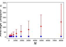
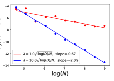
Figure 7: Illustration of the role of support recovery in the accuracy of $\mathrm{IJ}_{\backslash n}$ in the case of linear regression. Left: Points show the average of $\lvert\operatorname{supp}\hat{\theta}_{\backslash n}\rvert$ over random values of $n$. Error bars show the min and max $\lvert\operatorname{supp}\hat{\theta}_{\backslash n}\rvert$ over these $n$. For $\lambda=10.0\sqrt{\log(D)/N}$ (blue), the mean recovered support is constant with $N$. For $\lambda=1.0\sqrt{\log(D)/N}$ (red), $\lvert\operatorname{supp}\hat{\theta}_{\backslash n}\rvert$ grows with $N$, and varies dramatically for different values of $n$. Right: Percent error (Eq. 10) as $D$ scales with $N$. When the support recovery is constant, we recover an error scaling of roughly $1/N^{2}$, whereas a growing support results in a much slower decay.

That the approximation quality relies so heavily on the exact setting of $\lambda$ is somewhat concerning. However, we emphasize that sensitivity exists for $\ell_{1}$ regularization in general; as previously noted, Wainwright [2009] demonstrated similarly drastic behavior of $\operatorname{supp}\hat{\theta}$ in the same exact linear regression setup that we use here. On the other hand, Homrighausen and McDonald [2014] do show that using exact LOOCV to select $\lambda$ for $\ell_{1}$ regularized linear regression gives reasonable results. In Appendix H, we empirically show this is sometimes, but not always, the case for our and other approximate CV methods.

Accuracy of approximate CV by optimization error.

In early experiments, we used the Python bindings for the glmnet package [Friedman et al., 2009] to solve our $\ell_{1}$ regularized problems. However, we found that both $\mathrm{IJ}_{\backslash n}$ and $\mathrm{NS}_{\backslash n}$ failed to recover the roughly $1/N^{2}$ scaling present in fixed-dimensional problems (e.g. as shown in Fig. 1 of Section 1) that we would expect given our theoretical results. We found that this was due to the relatively loose convergence tolerance with which glmnet is implemented (e.g. parameter changes of $\leq 1\times 10^{-4}$ between iterations), which seems to be an issue for approximate CV methods and related approximations [Giordano et al., 2019b, 2015]. We implemented our own $\ell_{1}$ solver in Python using many of the speed-ups proposed in Friedman et al. [2009] and set a convergence theshold of $1\times 10^{-10}$ for the initial fit of $\hat{\theta}$. This solver was used to produce all of our results, including Fig. 7, which shows the expected roughly $1/N^{2}$ accuracy of $\mathrm{IJ}_{\backslash n}$ in blue.

Appendix G Details of real experiments

We use three publicly available datasets for our real-data experiments in Section 5:

1. The “Gisette” dataset Guyon et al. [2004] is available from the UCI repository at https://archive.ics.uci.edu/ml/datasets/Gisette. The dataset is constructed from the MNIST handwritten digits dataset. Specifically, the task is to differentiate between handwritten images of either “4” or “9.” There are $N=6,000$ training examples, each of which has $D=5,000$ features, some of which are junk “distractor features” added to make the problem more difficult.

2. The “bcTCGA” bcTCGA [2018] is a dataset of breast cancer samples from The Cancer Genome Atlas, which we downloaded from http://myweb.uiowa.edu/pbreheny/data/bcTCGA.html. The dataset consists of $N=536$ samples of tumors, each of which has the real-valued expression levels of $D=17,322$ genes. The task is to predict the real-valued expression level of the BRCA1 gene, which is known to correlate with breast cancer.

3. The “RCV1” dataset Lewis et al. [2004] is a dataset of Reuters’ news articles given one of four categorical labels according to their subject: “Corporate/Industrial,” “Economics,” “Government/Social,” and “Markets.” We use a pre-processed binarized version from https://www.csie.ntu.edu.tw/~cjlin/libsvmtools/datasets/binary.html, which combines the first two categories into a “positive” label and the latter two into a “negative” label. The full dataset contains $N=20,242$ articles, each of which has $D=47,236$ features. Running exact CV on this dataset would have been prohibitively slow, so we created a smaller dataset. First, the covariate matrix $X$ is extremely sparse (i.e., most entries are zero), so we selected the top 10,000 most common features and threw away the rest. We then randomly chose 5,000 documents to keep as our training set. After throwing away any of the 10,000 features that were now not observed in this subset, we were left with a dataset of size $N=5,000$ and $D=9,836$.

In order to run $\ell_{1}$ regularized regression on each of these datasets, we first needed to select a value of $\lambda$. Since all of these datasets are fairly high dimensional, our experiments in Appendix H suggests our approximation will be inaccurate for values of $\lambda$ that are “too small.” In an attempt to get the order of magnitude for $\lambda$ correct, we used the theoretically motivated value of $\lambda=C\sqrt{\log(D)/N}$ for some constant $C$ (e.g., Li et al. [2015] shows this scaling of $\lambda$ will recover the correct support for both linear and logistic regression). Section 5 suggests that the constant $C$ can be very important for the accuracy of our approximation, and our experiments there suggest that inaccuracy is caused by too large a recovered support size $\lvert\operatorname{supp}\hat{\theta}\rvert$. For the RCV1 and Gisette datasets, both run with logistic regression, we guessed a value of $C=1.5$, as this sits roughly in the range of values that give support recovery for logistic regression on synthetic datasets. After confirming that $\lvert\operatorname{supp}\hat{\theta}\rvert$ was not too large (i.e., of size ten or twenty), we proceeded with these experiments. Although we found linear regression on synthetic data typically needed a larger value of $C$ than logistic regression on synthetic data, we found that $C=1.5$ also produced reasonable results for the bcTCGA dataset.

Appendix H Selection of $\lambda$

Our work in this paper is almost exclusively focused on approximating CV for model assessment. However, this is not the only use-case of CV. CV is also commonly used for model selection, which, as a special case, contains hyperparameter tuning. Previous authors have used approximate CV methods for hyperparameter tuning in the way one might expect: for various values of $\lambda$, compute $\hat{\theta}$ and then use approximate CV to compute the out-of-sample error of each $\hat{\theta}$; the $\lambda$ leading to the lowest out-of-sample error is then selected [Obuchi and Kabashima, 2016, 2018, Beirami et al., 2017, Rad and Maleki, 2020, Wang et al., 2018, Giordano et al., 2019b]. While many of these authors theoretically study the accuracy of approximate CV, we note that they only do so in the context of model assessment and only empirically study approximate CV for hyperparameter tuning. In this appendix, we add to these experiments by showing that approximate CV can exhibit previously undemonstrated complex behavior when used for hyperparameter tuning.

We generate two synthetic $\ell_{1}$ regularized logistic regression problems with $N=300$ observations and $D=\{75,150\}$ dimensions. The matrix of covariates $X$ has i.i.d. $N(0,1)$ entries, and the true $\theta^{*}$ has its first five entries drawn i.i.d. as $N(0,1)$ with the rest set to zero. As a measure of the true out of sample error, we construct a test set with ten thousand observations. For a range of values of $\lambda$, we find $\hat{\theta}$, and measure the train, test, exact LOOCV, and approximate LOOCV errors via both $\mathrm{NS}_{\backslash n}$ and $\mathrm{IJ}_{\backslash n}$; the results are plotted in Fig. 8. $\mathrm{NS}_{\backslash n}$ (blue dashed curve) is an extremely close approximation to exact CV (red curve) in both datasets and selects a $\lambda$ that gives a test error very close to the $\lambda$ selected by exact CV. On the other hand, $\mathrm{IJ}_{\backslash n}$ (solid blue curve) performs very differently on the two datasets. For $D=75$, it selects a somewhat reasonable value for $\lambda$; however, for $D=150$, $\mathrm{IJ}_{\backslash n}$ goes disastrously wrong by selecting the obviously incorrect value of $\lambda=0$. While the results in Fig. 8 come from using our $\mathrm{IJ}_{\backslash n}$ to approximate CV for an $\ell_{1}$ regularized problem, we note that this issue is not specific to the current work; we observed similar behavior when using $\ell_{2}$ regularization and the pre-existing $\widetilde{\mathrm{IJ}}_{\setminus n}(\ell_{2})$.

While $\mathrm{NS}_{\backslash n}$ performs far better than $\mathrm{IJ}_{\backslash n}$ in the experiments here, it too has a limitation when $D>N$. In particular, when $\lambda$ is small enough, we will eventually recover $\lvert\hat{S}\rvert=N$. At this point, the matrix we need to invert in the definition of $\mathrm{NS}_{\backslash n}$ in Eq. 5 will be a $N\times N$ matrix that is the sum of $N-1$ rank-one matrices. As such, it will not be invertible, meaning that we cannot compute $\mathrm{NS}_{\backslash n}$ for small $\lambda$ when $D>N$. Even when $D$ is less than – but still close to – $N$, we have observed numerical issues in computing $\mathrm{NS}_{\backslash n}$ when $\lambda$ is sufficiently small; typically, these issues show up as enormously large values for ALOO for small values of $\lambda$.

Given the above discussion, we believe that an understanding of the behavior of $\mathrm{IJ}_{\backslash n}$ and $\mathrm{NS}_{\backslash n}$ for the purposes of hyperparameter tuning is a very important direction for future work.

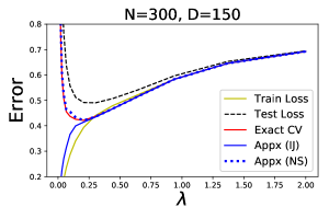
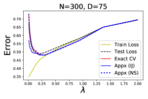
Figure 8: Experiment for selecting $\lambda$ from Appendix H. (Top:) Despite being very accurate for higher values of $\lambda$, the degredation of the accuracy of $\mathrm{IJ}_{\backslash n}$ for lower values of $\lambda$ (which corresponds to a larger $\hat{S}$) causes the selection of a $\lambda$ that is far from optimal in terms of test loss. (Bottom:) For a lower dimensional problem, the curve constructed by $\mathrm{IJ}_{\backslash n}$ much more closely mirrors that of exact CV for all values of $\lambda$. In both cases, $\mathrm{NS}_{\backslash n}$ performs well.

After the initial posting of this work, Wilson et al. [2020] provided a more thorough investigation of model selection using $\mathrm{NS}_{\backslash n}$ and $\mathrm{IJ}_{\backslash n}$. Their work gives an analytical example (as opposed to our empirical example here) showing that $\mathrm{IJ}_{\backslash n}$ can fail for model selection in sparse models. They further propose a modification to $\mathrm{IJ}_{\backslash n}$ based on proximal operators that avoids this issue in both theory and practice.

Appendix I Proofs from Section 4

As mentioned in the main text, there exist somewhat general assumptions in the $\ell_{1}$ literature under which $\operatorname{supp}\hat{\theta}=S$ [Lee et al., 2014, Li et al., 2015]. By taking these assumptions for all leave-one-out problems, we immediately get that $\operatorname{supp}\hat{\theta}_{\backslash n}=S$ for all $n$. Our method for proving Theorems 2 and 3 will be to show that the assumptions of those theorems imply those from the $\ell_{1}$ literature for all leave-one-out problems.

I.1 Assumptions from Li et al. [2015]

We choose to use the conditions from Li et al. [2015], as we find them easier to work with for our problem. Li et al. [2015] gives conditions on $F=(1/N)\sum_{n}f(x_{n}^{T}\theta,y_{n})$ under which $\operatorname{supp}\hat{\theta}=S$. We are interested in $\operatorname{supp}\hat{\theta}_{\backslash n}$, so we state versions of these conditions for $F^{\backslash n}:=(1/N)\sum_{m:\,m\neq n}f(x_{m}^{T}\theta,y_{n})$.

Assumption 10 (LSSC).

$\forall n$, $F^{\backslash n}$ satisfies the $(\theta^{*},\mathbb{R}^{D})$ locally structured smoothness condition (LSSC) with constant $K$. We recall this condition, due to Li et al. [2015], in Section I.2.

Assumption 11 (Strong convexity).

For a matrix $A$, let $\lambda_{min}(A)$ be the smallest eigenvalue of $A$. Then, $\forall n$ and for some constant $L_{min}$, the Hessian of $F^{\backslash n}$ is positive definite at $\theta^{*}$ when restricted to the dimensions in $S$: $\lambda_{min}\left(\nabla^{2}F^{\backslash n}(\theta^{*})_{SS}\right)\geq L_{min}>0.$

Assumption 12 (Incoherence).

$\forall n$ and for some $\gamma>0$,

$$\left\lVert\nabla^{2}F^{\backslash n}(\theta^{*})_{S^{c},S}\left(\nabla^{2}F^{\backslash n}(\theta^{*})_{SS}\right)^{-1}\right\rVert_{\infty}<1-\gamma.$$ (30)

Assumption 13 (Bounded gradient).

For $\gamma$ from Assumption 12, $\forall n$, the gradient of $F^{\backslash n}$ evaluated at the true parameters $\theta^{*}$ is small relative to the amount of regularization: $\left\lVert\nabla F^{\backslash n}(\theta^{*})\right\rVert_{\infty}\leq(\gamma/4)\lambda.$

Assumption 14 ($\lambda$ sufficiently small).

For $K,L_{min}$ and $\gamma$ as in Assumptions 10, 11 and 12, the regularization parameter is sufficiently small: $\lambda<L^{2}_{min}\gamma/(4(\gamma+4)^{2}D_{\mathrm{eff}}K),$ where there is no constraint on $\lambda$ if $K=0$.

We see in Section I.3 that a minor adaptation of Theorem 5.1 from Li et al. [2015] tells us that Assumptions 10, 11, 12, 13 and 14 imply $\forall n,\operatorname{supp}\hat{\theta}_{\backslash n}\subseteq S$. To prove the accuracy of $\mathrm{NS}_{\backslash n}$ and $\mathrm{IJ}_{\backslash n}$, though, we further need that $\operatorname{supp}\hat{\theta}_{\backslash n}\subseteq\hat{S}$ so that all LOOCV problems run over the same low-dimensional space as the full-data problem. It will be easier to state conditions for a stronger result, that $\operatorname{supp}\hat{\theta}_{\backslash n}=\hat{S}=S$. This will follow from an assumption on the smallest entry of $\theta^{*}_{S}$, which we stated as Assumption 4 in the main text. We stated Assumption 4 using the quantity $T_{min}$ to avoid stating Assumptions 11 and 12 in the main text. We can now state its full version.

Assumption 15 (full version of Assumption 4).

For $L_{min}$ and $\gamma$ from Assumptions 11 and 12, $\min_{s\in S}\lvert\theta^{*}_{s}\rvert>(\sqrt{D_{\mathrm{eff}}}(\gamma+4)/L_{min})\lambda.$

Proposition 5.

If Assumptions 10, 11, 12, 13, 14 and 15 hold, then $\forall n,\operatorname{supp}\hat{\theta}_{\backslash n}=\hat{S}=S$.

Proof.

This is immediate from Theorem 5.1 of Li et al. [2015]. ∎

I.2 Local structured smoothness condition (LSSC)

We now define the local structured smoothness condition (LSSC). The LSSC was introduced by Li et al. [2015] for the purpose of extending proof techniques for the support recovery of $\ell_{1}$ regularized linear regression to more general $\ell_{1}$ regularized $M$-estimators. Essentially, it provides a condition on the smoothness of the third derivatives of the objective $F(\theta)$ near the true sparse $\theta^{*}$. One can then analyze a second order Taylor expansion of the loss and use the LSSC to show that the remainder in this expansion is not too large. To formalize the LSSC, we need to define the third order derivative of $F$ evaluated along a direction $u\in\mathbb{R}^{D}$:

$$D^{3}F(\theta)[u]:=\lim_{t\to 0}\frac{\nabla^{2}F(\theta+tu)-\nabla^{2}F(\theta)}{t}.$$

In the cases considered in this paper, this is just a $D\times D$ matrix. We can then naturally define the scalar $D^{3}F(\theta)[u,v,w]$ as an outer product on this matrix:

$$D^{3}[u,v,w]:=v^{T}\big{(}D^{3}F(\theta)[u]\big{)}w$$

Definition 2 (LSSC).

Let $F:\mathbb{R}^{D}\to\mathbb{R}$ be a continuously three-times differentiable function. For $\theta^{*}\in\mathbb{R}^{D}$ and $N_{\theta^{*}}\subseteq\mathbb{R}^{D}$, the function $F$ satisfies the $(\theta^{*},N_{\theta^{*}})$ LSSC with constant $K\geq 0$ if for any $u\in\mathbb{R}^{D}$:

$$\lvert D^{3}f(\theta^{*}+\delta)[u,u,e_{j}]\rvert\leq K\left\lVert u\right\rVert_{2}^{2},$$ (31)

where $e_{j}\in\mathbb{R}^{D}$ is the $j$th coordinate vector, and $\delta\in\mathbb{R}^{D}$ is any vector such that $\theta^{*}+\delta\in N_{\theta^{*}}$.

We note that this definition is actually different from the original definition given in Li et al. [2015], who prove the two to be equivalent in their Proposition 3.1. Li et al. [2015] go on to prove bounds on the LSSC constants for linear and logistic regression, which we state as Proposition 11 and Proposition 13 below.

Note that Assumption 10 in the main text states that the LSSC holds with $N_{\theta^{*}}=\mathbb{R}^{D}$. We state Assumption 10 in this form purely for conciseness; we will only consider checking Assumption 10 for linear and logistic regression, both of which satisfy the LSSC with $N_{\theta^{*}}=\mathbb{R}^{D}$. Going beyond these cases, it is easily possible to state a version of our results with $N_{\theta^{*}}\neq\mathbb{R}^{D}$; however, this will require an extra assumption along the lines of Condition 7 of Theorem 5.1 in Li et al. [2015], which is trivially satisfied when $N_{\theta^{*}}=\mathbb{R}^{D}$. In order to avoid stating an extra assumption that is trivially satisfied in the cases we consider, we chose to simply state the LSSC with $N_{\theta^{*}}=\mathbb{R}^{D}$.

I.3 Assumptions 10, 11, 12, 13 and 14 imply $\operatorname{supp}\hat{\theta}_{\backslash n}\subseteq S$ for all $n$

Theorem 5.1 of Li et al. [2015] gives conditions on $F$ under which $\operatorname{supp}\hat{\theta}=S$. So, if these conditions hold for all $F^{\backslash n}$, then we have $\operatorname{supp}\hat{\theta}_{\backslash n}=S$ for all $n$. Their Theorem 5.1 actually has two extra assumptions beyond Assumptions 10, 11, 12, 13 and 14. The first is their Assumption 7; however, this is immediately implied by the fact that we assume the LSSC holds with $N_{\theta^{*}}=\mathbb{R}^{D}$. The second is their analogue of our Assumption 15; however, they use this condition to imply that $\hat{\theta}=S$ after having shown that $\hat{\theta}\subseteq S$.

I.4 Useful results for proving Theorems 2 and 3

Before going on to Theorems 2 and 3, we will give a few useful results. We first define a sub-Exponential random variable:

Definition 3 (Vershynin [2018]).

A random variable $V$ is $c_{x}$-sub-Exponential if $E[\exp(V/c_{x})]\leq 2$.

We will frequently use the fact that if $X$ is $c_{x}$-sub-Gaussian, then $X^{2}$ is $c_{x}^{2}$-sub-Exponential. Now we state a few existing results about the maxima of sub-Gaussian and sub-Exponential random variables that will be useful in our proofs.

Lemma 1 (Lemma 5.2 from van Handel [2016]).

Suppose that we have real valued random variables $Z_{1},\dots,Z_{N}$ that satisfy $\log E[e^{\lambda Z_{n}}]\leq\psi(\lambda)$ for all $n=1,\dots,N$ and all $\lambda\geq 0$ for some convex function $\psi:\mathbb{R}\to\mathbb{R}$ with $\psi(0)=\psi^{\prime}(0)=0$. Then for any $u\geq 0$ :

$$\Pr\left[\max_{n=1,\dots,N}Z_{n}\geq\psi^{*-1}(\log N+u)\right]\leq e^{-u}.$$

where $\psi^{*-1}$ is the inverse of the Legendre dual of $\psi$.

Remembering the definition of a sub-Gaussian random variable from Definition 1, Lemma 1 can be used to show the following:

Corollary 1.

Let $Z_{1},\dots,Z_{N}$ be i.i.d. sub-Gaussian random variables with parameter $c_{x}$. Then:

$$\Pr\left[\max_{n=1,\dots,N}Z_{n}\geq E[Z_{n}]+\sqrt{2Cc_{x}^{2}\log N}+u\right]\leq e^{-C\frac{u^{2}}{2c_{x}^{2}}}$$ (32)

$$\Pr\left[\max_{n=1,\dots,N}Z_{n}^{2}\geq E[Z_{n}^{2}]+Cc_{x}^{2}(\log N+1+u)\right]\leq e^{-u}$$ (33)

Proof.

For the first inequality, the definition of a sub-Gaussian random variable is that $\log Ee^{\lambda Z_{n}}\leq\lambda^{2}c_{x}/2=:\psi(\lambda)$, which has $\psi^{*}(y)=y^{2}/(2Cc_{x}^{2})$ and $\psi^{*-1}(x)=\sqrt{2Cc_{x}^{2}x}$. We use the upper bound:

$$\psi^{*-1}(\log N+u)=\sqrt{2Cc_{x}^{2}(\log N+u)}\leq\sqrt{2Cc_{x}^{2}\log N}+\sqrt{2Cc_{x}^{2}u},$$

Using this upper bound with Lemma 1 and changing variables $u\mapsto u^{2}/(2Cc_{x}^{2})$ gives the first inequality.

For the second inequality, use the fact that $Z_{n}^{2}$ is sub-Exponential with parameter $c_{x}^{2}$ so that it satisfies $\log Ee^{\lambda Z_{n}^{2}}\leq\psi(\lambda),$ where:

$$\psi(\lambda):=\begin{cases}\lambda Cc_{x}^{2},&0\leq t\leq 1/c_{x}^{2}\\ \infty,&\mathrm{o.w.}\end{cases}.$$

For $x\geq 0$, this $\psi$ has inverse Legendre dual $\psi^{*-1}(x)=Cc_{x}^{2}(x+1)$. Plugging into Lemma 1 gives the result. ∎

Proposition 6.

Let $x_{1},\dots,x_{N}$ be random vectors in $\mathbb{R}^{D}$ with i.i.d. $c_{x}$-sub-Gaussian components and $E[x_{nd}^{2}]=1$. Then:

$$\Pr\left[\max_{n=1,\dots,N}\left\lVert x_{n}\right\rVert_{2}\geq\sqrt{D}+\sqrt{2Cc_{x}^{4}\log N}+u\right]\leq e^{-C\frac{u^{2}}{2c_{x}^{4}}},$$ (34)

where $C>0$ is some global constant, independent of $c_{x},D,$ and $N$.

Proof.

From Theorem 3.1.1 of Vershynin [2018], we have that $\left\lVert x_{n}\right\rVert_{2}-\sqrt{D}$ is sub-Gaussian with parameter $Cc_{x}^{2}$, where $C$ is some constant. Using the first part of Corollary 1 gives the result. ∎

I.5 Proof of Theorem 2 (Linear Regression)

Recall Assumptions 1 and 5: we assume a linear regression model $y_{n}=x_{n}^{T}\theta^{*}+\varepsilon_{n}$, where $x_{n}\in\mathbb{R}^{D}$ has i.i.d. $c_{x}$-sub-Gaussian components with $E[x_{nd}^{2}]=1$ and $\varepsilon_{n}$ is $c_{\varepsilon}$-sub-Gaussian. For notation throughout this section, we will let $C$ denote an absolute constant independent of any aspect of the problem ($N,D,D_{\mathrm{eff}},c_{x},$ or $c_{\varepsilon}$) that will change from line to line (e.g. we may write $5C^{2}=C$). We will frequently use $X_{\cdot,S}$ to denote the $N\times D_{\mathrm{eff}}$ matrix formed by taking the columns of $X$ that are in $S$, $x_{nS}$ to denote the coordinates of the $n$th vector of covariates $x_{n}$ that are in the set $S$, and $X_{\backslash n,S}$ to denote the matrix $X_{\cdot,S}$ with the $n$th row removed. We will show the following theorem, stated more concisely as Theorem 2 in the main text:

Theorem 4 (Restated version of Theorem 2 from main text).

Take Assumptions 1, 2, 5, 3 and 15. Suppose the regularization parameter $\lambda$ satisfies:

$$\lambda\geq\frac{1}{\alpha-M_{\mathrm{lin}}}\sqrt{\frac{c_{x}^{2}c_{\varepsilon}^{2}\log D}{NC}+\frac{25c_{x}^{2}c_{\varepsilon}^{2}}{NC}}+\frac{4c_{x}c_{\varepsilon}(\log(ND)+26)}{N(\alpha-M_{\mathrm{lin}})},$$ (35)

where $C$ is a constant in $N,D,D_{\mathrm{eff}},c_{x}$ and $c_{\varepsilon}$, and $M_{\mathrm{lin}}$ is defined as:

$$M_{\mathrm{lin}}=$$

$$\quad\frac{CD_{\mathrm{eff}}\left(\sqrt{50c_{x}^{2}}+\sqrt{2c_{x}^{2}\log(N(D-D_{\mathrm{eff}}))}\right)\left(\sqrt{D_{\mathrm{eff}}}+\sqrt{50c_{x}^{4}}+\sqrt{2c_{x}^{4}\log N}\right)}{N-3c_{x}^{2}\sqrt{N}\big{(}\sqrt{D_{\mathrm{eff}}}+5\big{)}}+$$

$$\quad\frac{CD_{\mathrm{eff}}\left(D_{\mathrm{eff}}+D_{\mathrm{eff}}c_{x}^{2}(\log N+26)\right)\left(\sqrt{N}+\sqrt{50c_{x}^{4}}+\sqrt{2c_{x}^{4}\log(D-D_{\mathrm{eff}})}\right)\left(\sqrt{ND_{\mathrm{eff}}}+\sqrt{50c_{x}^{4}}\right)}{\big{(}N-3c_{x}^{2}\sqrt{N}\big{(}\sqrt{D_{\mathrm{eff}}}+5\big{)}\big{)}^{2}}$$ (36)

Then for $N$ sufficiently large, Condition 1 holds with probability at least $1-26e^{-25}$, where the probability is over the random data $\{(x_{n},y_{n})\}_{n=1}^{N}$.

Proof.

For a fixed regularization parameter $\lambda$ and random data $\{x_{n},y_{n}\}_{n=1}^{N}$, we are interested in the probability that any of Assumptions 10, 11, 12, 13 and 14 are violated, as Proposition 5 then proves the result. For convenience in writing the incoherence condition, define $J_{nd}\in\mathbb{R}^{D}$, for $d\in S^{c}$, as:

$$J_{nd}:=\left(X_{\backslash n,S}^{T}X_{\backslash n,S}\right)^{-1}X_{\backslash n,S}^{T}X_{\backslash n,d}.$$ (37)

It is easiest to show that each of Assumptions 10, 11, 12, 13 and 14 hold with high probability separately, rather than all together, so we apply a union bound to get:

$$\Pr \left[\mathrm{any\ assumption\ violated}\right]\leq$$

$$\Pr\left[\min_{n}\lambda_{min}(X_{\backslash n,S}^{T}X_{\backslash n,S})=0\right]$$

$$+\Pr\left[\max_{n}\max_{d\in S^{c}}\left\lVert J_{nd}\right\rVert_{1}\geq 1\right]$$

$$+\Pr\left[\max_{n}\left\lVert\nabla F_{\backslash n}\right\rVert_{\infty}>\frac{\lambda\big{(}1-\max_{n}\max_{d\in S^{c}}\left\lVert J_{nd}\right\rVert_{1}\big{)}}{4}\right]$$

$$+\Pr\left[\frac{\min_{n}\lambda_{min}^{2}(X_{\backslash n,S}^{T}X_{\backslash n,S})}{4\left(\big{(}1-\max_{n}\max_{d\in S^{c}}\left\lVert J_{nd}\right\rVert_{1}\big{)}+4\right)^{2}}\frac{\big{(}1-\max_{n}\max_{d\in S^{c}}\left\lVert J_{nd}\right\rVert_{1}\big{)}}{D_{\mathrm{eff}}K}\leq\lambda\right]$$

We will bound each term by appealing to the Lemmas and Propositions proved below. Using Lemma 2 and Lemma 4, the first and third terms are bounded by $16^{-25}$. As noted in Proposition 11, we have $\Pr[K=0]=1$, so the final probablity is equal to zero (as the event reduces to $\infty<\lambda$). To bound the second probability, we have that Lemma 3 says that:

$$\Pr\left[\max_{n}\max_{d\in S^{c}}\left\lVert J_{nd}\right\rVert_{1}\geq 1-\alpha+M_{\mathrm{lin}}\right]\leq 9e^{-25}.$$

As $\alpha>0$, if $M_{\mathrm{lin}}=o(1)$ as $N\to\infty$, we will we have that $1-\alpha+M_{\mathrm{lin}}<1$ for large enough $N$. This would imply the third probability is $\leq 9e^{-25}$ for $N$ large enough. Under our conditions on the growth of $D_{\mathrm{eff}}$ and $D$, we can show that $M_{\mathrm{lin}}=o(1)$. We have, hiding constants and lower order terms in $N,D,$ and $D_{\mathrm{eff}}$:

$$M_{\mathrm{lin}} =O\left(\frac{D_{\mathrm{eff}}\sqrt{\log(N)+\log(D)}\left(\sqrt{D_{\mathrm{eff}}}+\sqrt{\log(N)}\right)}{N-\sqrt{ND_{\mathrm{eff}}}}+\frac{D_{\mathrm{eff}}^{5/2}\log(N)\left(\sqrt{N}+\sqrt{\log(D)}\right)\sqrt{N}}{(N-\sqrt{ND_{\mathrm{eff}}})^{2}}\right)$$

$$=O\left(\frac{D_{\mathrm{eff}}\left(\sqrt{D_{\mathrm{eff}}\log(N)}+\sqrt{D_{\mathrm{eff}}\log(D)}+\log(N)+\sqrt{\log(N)\log(D)}\right)}{N-\sqrt{ND_{\mathrm{eff}}}}+\frac{D_{\mathrm{eff}}^{5/2}N\log(N)}{(N-\sqrt{ND_{\mathrm{eff}}})^{2}}\right),$$ (38)

where the second statement follows from using $\sqrt{\log(N)+\log(D)}\leq\sqrt{\log(N)}+\sqrt{\log(D)}$ and $D=o(e^{N})$. Now, given that $D_{\mathrm{eff}}=o([N/\log(N)]^{2/5})$, the second term in Eq. 38 is $o(1)$. The first term is also $o(1)$ by combining $D_{\mathrm{eff}}=o([N/\log(N)]^{2/5})$ with $D_{\mathrm{eff}}^{3/2}\sqrt{\log(D)}=o(N)$. Thus, $M_{\mathrm{lin}}=o(1)$, which completes the proof. ∎

What remains is to prove Lemmas 2, 4, 3 and 11 needed to prove Theorem 4. We do this in the following four subsections.

I.6 Linear regression: minimum eigenvalue

All we want to bound right now is the probability that the minimum eigenvalue is actually equal to zero; however, it will be useful later to show that it is $\Omega(N)$ with high probability. The lemma we prove in this section shows exactly this. We will start with two propositions.

Proposition 7.

If $X_{\cdot,S}$ is an $N\times D_{\mathrm{eff}}$ matrix with independent $c_{x}$-sub-Gaussian entries with unit second moments, then:

$$\Pr\left[\lambda_{min}(X_{\cdot,S}^{T}X_{\cdot,S})\leq N-2Cc_{x}^{2}\sqrt{N}(\sqrt{D_{\mathrm{eff}}}+5)\right]\leq 2e^{-25},$$ (39)

where $C>0$ is a global constant.

Proof.

Theorem 4.6.1 of Vershynin [2018] gives a concentration inequality for the minimum singular value, $s_{min}(X_{\cdot,S})$, of $X_{\cdot,S}$:

$$\Pr\left[s_{min}(X_{\cdot,S})\leq\sqrt{N}-Cc_{x}^{2}(\sqrt{D_{\mathrm{eff}}}+t)\right]\leq 2e^{-t^{2}}.$$ (40)

Using the fact that the minimum eigenvalue of $X_{\cdot,S}^{T}X_{\cdot,S}$ is the square of the minimum singular value of $X_{\cdot,S}$ and putting in $t=5$:

$$\Pr\left[\lambda_{min}(X_{\cdot,S}^{T}X_{\cdot,S})\leq N-2Cc_{x}^{2}\sqrt{N}(\sqrt{D_{\mathrm{eff}}}+5)+C^{2}c_{x}^{4}(\sqrt{D_{\mathrm{eff}}}+5)^{2}\right]\leq 2e^{-25}.$$

Dropping the $C^{2}c_{x}^{4}(\sqrt{D_{\mathrm{eff}}}+5)^{2}$ gives the result. ∎

Proposition 8.

If $X_{\backslash n,S}$ is the $N-1\times D_{\mathrm{eff}}$ matrix formed by removing the $n$th row from $X_{\cdot,S}$, we have:

$$\lambda_{min}(X_{\backslash n,S}^{T}X_{\backslash n,S})\geq\lambda_{min}(X_{\cdot,S}^{T}X_{\cdot,S})-\left\lVert x_{nS}\right\rVert_{2}^{2},$$ (41)

where $x_{n}$ is the $n$th row of $X_{\cdot,S}$.

Proof.

Looking at the variational characterization of the minimum eigenvalue:

$$\lambda_{min}(X_{\backslash n,S}^{T}X_{\backslash n,S}) =\min_{z\in\mathbb{R}^{D_{\mathrm{eff}}}\,:\,\left\lVert z\right\rVert_{2}=1}\bigg{[}z^{T}X_{\cdot,S}^{T}X_{\cdot,S}z-z^{T}x_{nS}x_{nS}^{T}z\bigg{]}$$

$$\geq\min_{z}z^{T}X_{\cdot,S}^{T}X_{\cdot,S}z-\max_{z}z^{T}x_{nS}x_{nS}^{T}z$$

$$=\lambda_{min}(X_{\cdot,S}^{T}X_{\cdot,S})-\left\lVert x_{nS}\right\rVert_{2}^{2}.$$

∎

The above two propositions now allow us to prove the bound we want on $\min_{n}\lambda_{min}(X_{\backslash n,S}^{T}X_{\backslash n,S})$. In the following lemma, we will assume that $D_{\mathrm{eff}}=o(N/\log(N))$. While we ultimately will have the more restrictive requirement that $D_{\mathrm{eff}}=o([N/\log(N)]^{2/5})$ in Assumption 3, the current result can be stated with the less restrictive requirement of $o(N/\log(N))$.

Lemma 2.

Suppose $X_{\cdot,S}$ is a $N\times D_{\mathrm{eff}}$ matrix with independent $c_{x}$-sub-Gaussian entries and $D_{\mathrm{eff}}$ is $o(N/\log(N))$ as function of $N$. Then we have for $N$ sufficiently large:

$$\Pr\left[\min_{n=1,\dots N}\lambda_{min}(X_{\backslash n,S}^{T}X_{\backslash n,S})\leq N-3Cc_{x}^{2}\sqrt{N}\big{(}\sqrt{D_{\mathrm{eff}}}+5\big{)}\right]\leq 3e^{-25}$$ (42)

Proof.

In what follows, and repeatedly throughout the rest of our proofs, we will make use of the following generic inequality for any events $A$ and $B$:

$$\Pr[A] =\Pr[A\mid B]\Pr[B]+\Pr[A\mid B^{c}]\Pr[B^{c}]$$

$$\leq\Pr[A\mid B]Pr[B]+\Pr[B^{c}],$$ (43)

Calling the probability on the left hand side of Eq. 42 $P$, we can break $P$ down as, for some constant $L_{min}$:

$$P \leq$$

$$\Pr\left[\min_{n=1,\dots N}\lambda_{min}(X_{\backslash n,S}^{T}X_{\backslash n,S})\leq N-3Cc_{x}^{2}\sqrt{N}\big{(}\sqrt{D_{\mathrm{eff}}}+5\big{)}\;\;\bigg{|}\;\;\lambda_{min}(X_{\cdot,S}^{T}X_{\cdot,S})\geq L_{min}\right]\Pr\left[\lambda_{min}(X_{\cdot,S}^{T}X_{\cdot,S})\geq L_{min}\right]$$

$$\quad\quad\quad\quad\quad\quad+\Pr\left[\lambda_{min}(X_{\cdot,S}^{T}X_{\cdot,S})\leq L_{min}\right]$$

$$\leq\Pr\left[\min_{n=1,\dots N}L_{min}-\left\lVert x_{nS}\right\rVert_{2}^{2}\leq N-3Cc_{x}^{2}\sqrt{N}\big{(}\sqrt{D_{\mathrm{eff}}}+5\big{)}\;\;\bigg{|}\;\;\lambda_{min}(X_{\cdot,S}^{T}X_{\cdot,S})\geq L_{min}\right]\Pr\left[\lambda_{min}(X_{\cdot,S}^{T}X_{\cdot,S})\geq L_{min}\right]$$

$$\quad\quad\quad\quad\quad\quad+\Pr\left[\lambda_{min}(X_{\cdot,S}^{T}X_{\cdot,S})\leq L_{min}\right]$$

$$\leq\Pr\left[\max_{n}\left\lVert x_{nS}\right\rVert^{2}_{2}\geq L_{min}-N+3Cc_{x}^{2}\sqrt{N}\big{(}\sqrt{D_{\mathrm{eff}}}+5\big{)}\right]+\Pr\left[\lambda_{min}(X_{\cdot,S}^{T}X_{\cdot,S})\leq L_{min}\right]$$

Picking $L_{min}=N-2Cc_{x}^{2}\sqrt{N}\big{(}\sqrt{D_{\mathrm{eff}}}+5\big{)}$, we have that the second probability at most $2e^{-25}$ by Proposition 8. Now to control the $\max_{n}\|x_{nS}\|_{2}^{2}$, note that $\|x_{nS}\|_{2}^{2}$ is $D_{\mathrm{eff}}c_{x}^{2}$-sub-Exponential, and choose $u=25$ in the second statement of Corollary 1; this tells us that the first probability is at most $e^{-25}$ if $E[\left\lVert x_{nS}\right\rVert_{2}^{2}]+Cc_{x}^{2}(\log N+26)=D_{\mathrm{eff}}+Cc_{x}^{2}(\log N+26)$ is less than $Cc_{x}^{2}\sqrt{N}\big{(}\sqrt{D_{\mathrm{eff}}}+5\big{)}$, which, for $D_{\mathrm{eff}}$ being $o(N/\log(N))$, is satisfied for $N$ large enough. ∎

I.7 Linear regression: incoherence

The following proposition will be useful in proving Lemma 3 below:

Proposition 9.

Let $z\in\mathbb{R}^{N}$ be any vector and $z_{\backslash n}\in\mathbb{R}^{N-1}$ the same vector with the $n$th coordinate removed. Also let $X_{\cdot,S}\in\mathbb{R}^{N\times D_{\mathrm{eff}}}$ be some matrix with $X_{\backslash n,S}$ the same matrix with the $n$th row removed. Define, for any vector $z\in R^{N}$:

$$J_{nz}:=\left(X_{\backslash n,S}^{T}X_{\backslash n,S}\right)^{-1}X_{\backslash n,S}^{T}z_{\backslash n},$$ (44)

and $J_{z}$ the same but with no row removed. Then:

$$\left\lVert J_{nz}-J_{z}\right\rVert_{1}\leq D_{\mathrm{eff}}\frac{\lvert z_{n}\rvert\left\lVert x_{nS}\right\rVert_{2}}{\lambda_{min}\big{(}X_{\backslash n,S}^{T}X_{\backslash n,S}\big{)}}$$

$$+D_{\mathrm{eff}}\frac{\left\lVert x_{nS}\right\rVert_{2}^{2}}{\lambda_{min}^{2}\big{(}X_{\backslash n,S}^{T}X_{\backslash n,S}\big{)}}\left\lVert z\right\rVert_{2}\left\lVert X_{\cdot,S}\right\rVert_{2},$$

where $\left\lVert X_{\cdot,S}\right\rVert_{2}:=\sqrt{\sum_{n=1}^{N}\sum_{s\in S}X_{ns}^{2}}$.

Proof.

We can rewrite $J_{z}=(X_{\cdot,S}^{T}X_{\cdot,S})^{-1}X_{\cdot,S}^{T}z$ by noting that $X_{\cdot,S}^{T}X_{\cdot,S}$ and $X_{\backslash n,S}^{T}X_{\backslash n,S}$ differ by a rank one update and then applying the Sherman-Morrison formula:

$$J_{z} =(X_{\cdot,S}^{T}X_{\cdot,S})^{-1}X_{\cdot,S}^{T}z$$ (45)

$$=\left((X_{\backslash n,S}^{T}X_{\backslash n,S})^{-1}-\frac{(X_{\backslash n,S}^{T}X_{\backslash n,S})^{-1}x_{nS}x_{nS}^{T}(X_{\backslash n,S}^{T}X_{\backslash n,S})^{-1}}{1+x_{nS}^{T}(X_{\backslash n,S}^{T}X_{\backslash n,S})^{-1}x_{nS}}\right)X_{\cdot,S}^{T}z$$ (46)

$$=\left(J_{nz}+(X_{\backslash n,S}^{T}X_{\backslash n,S})^{-1}x_{nS}z_{n}\right)-\frac{(X_{\backslash n,S}^{T}X_{\backslash n,S})^{-1}x_{nS}x_{nS}^{T}(X_{\backslash n,S}^{T}X_{\backslash n,S})^{-1}}{1+x_{nS}^{T}(X_{\backslash n,S}^{T}X_{\backslash n,S})^{-1}x_{nS}}X_{\cdot,S}^{T}z$$ (47)

To cleanup notation a bit, let $B:=X_{\backslash n,S}^{T}X_{\backslash n,S}$. We can continue to rewrite the above as:

$$=\left(J_{nz}+B^{-1}x_{nS}z_{n}\right)-\frac{B^{-1}x_{nS}}{1+x_{nS}^{T}B^{-1}x_{nS}}\sum_{m=1}^{N}z_{m}x_{nS}^{T}B^{-1}x_{mS}$$ (48)

Now, we are interested in $\left\lVert J_{nz}-J_{z}\right\rVert_{1}$, which we will bound by subtracting $J_{nz}$ from both sides of the above equation and then examine each coordinate by multiplying by the $i$th unit vector $e_{i}$:

$$\lvert e_{i}^{T}(J_{nz}-J_{z})\rvert \leq\lvert e_{i}^{T}B^{-1}x_{nS}\rvert\lvert z_{n}\rvert+\frac{\lvert e_{i}^{T}B^{-1}x_{nS}\rvert}{1+x_{nS}^{T}B^{-1}x_{nS}}\sum_{m=1}^{N}\lvert z_{m}\rvert\lvert x_{nS}^{T}B^{-1}x_{mS}\rvert$$ (49)

$$\leq\lvert z_{n}\rvert\lambda_{max}(B^{-1})\left\lVert x_{nS}\right\rVert_{2}+\frac{\lambda^{2}_{max}(B^{-1})\left\lVert x_{nS}\right\rVert_{2}^{2}}{1+\lambda_{min}(B^{-1})\left\lVert x_{nS}\right\rVert^{2}_{2}}\sum_{m=1}^{N}\lvert z_{m}\rvert\left\lVert x_{mS}\right\rVert_{2}$$ (50)

The $\lambda_{min}(B^{-1})\left\lVert x_{nS}\right\rVert_{2}^{2}$ is strictly positive, so we can drop it from the denominator for a further upper bound. Using the fact that, for the positive semidefinite matrix $B$ we have $\lambda_{min}(B^{-1})=1/\lambda_{max}(B)$ and $\lambda_{max}(B^{-1})=1/\lambda_{min}(B)$, we get:

$$\lvert e_{i}^{T}(J_{nz}-J_{z})\rvert\leq\frac{\lvert z_{n}\rvert\left\lVert x_{nS}\right\rVert_{2}}{\lambda_{min}(B)}+\frac{\left\lVert x_{nS}\right\rVert_{2}^{2}}{\lambda^{2}_{min}(B)}\sum_{m=1}^{N}\lvert z_{m}\rvert\left\lVert x_{mS}\right\rVert_{2}.$$ (51)

Finally, use Cauchy-Schwarz to get $\sum_{m=1}^{N}\lvert z_{m}\rvert\left\lVert x_{mS}\right\rVert_{2}\leq\left\lVert z\right\rVert_{2}\left\lVert X_{\cdot,S}\right\rVert_{2}$, where $\left\lVert X_{\cdot,S}\right\rVert_{2}:=\left(\sum_{m=1}^{N}\sum_{s\in S}x_{ms}^{2}\right)^{1/2}$. Notice that our upper bound is now independent of the index $i$; this means we have a bound on any coordinate $i$ of $\lvert(J_{nz}-J_{z})\rvert$. So, multiplying this bound by $D_{\mathrm{eff}}$ upper bounds $\left\lVert J_{nz}-J_{z}\right\rVert_{1}$, which gives the result. ∎

To get a high probability upper bound on $\left\lVert J_{nd}\right\rVert_{1}$, the idea will be to use $\|J_{nd}\|_{1}\leq\|J_{d}\|_{1}+\|J_{nd}-J_{d}\|_{1}$, and then put high probability bounds on the bound given by Proposition 9.

Lemma 3.

Take Assumptions 1, 2 and 5. Then, for the scalar $M_{\mathrm{lin}}$ defined in Theorem 2, we have:

$$\Pr\left[\max_{n=1,\dots,N}\max_{d\in S^{c}}\left\lVert J_{nd}\right\rVert_{1}\geq 1-\alpha+M_{\mathrm{lin}}\right]\leq 10e^{-25},$$ (52)

where $J_{nd}$ is defined in Eq. 37 above.

Proof.

First, for any $n$ and $d$, we have $\|J_{nd}\|_{1}\leq\|J_{d}\|_{1}+\|J_{nd}-J_{d}\|_{1}$. We can upper bound $\|J_{nd}-J_{d}\|_{1}$ using Proposition 9 and then apply a high probability upper bound. Following the same idea of conditioning and peeling off terms as in the proof of Lemma 2, we can condition on the following events, the complement of each of which has a small constant probability:

$$\left\{\min_{n}\lambda_{min}(X_{\backslash n,S}^{T}X_{\backslash n,S})\geq N-3Cc_{x}^{2}\sqrt{N}\big{(}\sqrt{D_{\mathrm{eff}}}+5\big{)}\right\}$$ (53)

$$\left\{\left\lVert X_{\cdot,S}\right\rVert_{2}\leq\sqrt{ND_{\mathrm{eff}}}+\sqrt{50Cc_{x}^{4}}\right\}$$ (54)

$$\left\{\max_{n}\left\lVert x_{nS}\right\rVert_{2}\leq\sqrt{D_{\mathrm{eff}}}+\sqrt{50Cc_{x}^{4}}+\sqrt{2Cc_{x}^{4}\log N}\right\}$$ (55)

$$\left\{\max_{d\in S^{c}}\left\lVert X_{\cdot,d}\right\rVert_{2}\leq\sqrt{N}+\sqrt{50Cc_{x}^{4}}+\sqrt{2Cc_{x}^{4}\log(D-D_{\mathrm{eff}})}\right\}$$ (56)

$$\left\{\max_{n}\max_{d\in S^{c}}\lvert x_{n,d}\rvert\leq\sqrt{50Cc_{x}^{2}}+\sqrt{2c_{x}^{2}\log(N(D-D_{\mathrm{eff}}))}\right\}$$ (57)

$$\left\{\max_{n}\left\lVert x_{nS}\right\rVert_{2}^{2}\leq D_{\mathrm{eff}}+c_{x}^{2}D_{\mathrm{eff}}(\log N+26)\right\}$$ (58)

The probability of the complement of the first event is $\leq 3e^{-25}$ by Lemma 2, the second is $\leq e^{-25}$ by noting that $\left\lVert X_{\cdot,S}\right\rVert_{2}-\sqrt{ND_{\mathrm{eff}}}$ is a $Cc_{x}^{2}$-sub-Gaussian random variable and applying a standard sub-Gaussian bound, the third is $\leq e^{-25}$ by applying Proposition 6, the fourth is $\leq e^{-25}$ by the same reasoning as the third, and the fifth is $\leq 2e^{-25}$ by the first part of Corollary 1. Finally, the sixth is $\leq e^{-25}$ by noting that $\|x_{nS}\|_{2}^{2}$ is a $c_{x}^{2}D_{\mathrm{eff}}$-sub-Exponential random variable, to which we can apply Corollary 1. All in all, these probabilities sum up to $9e^{-25}$. Conditioned on all these events, we can upper bound the upper bound on $\left\lVert J_{nd}-J_{d}\right\rVert_{1}$ given by Proposition 9 to get:

$$\left\lVert J_{nd}-J_{d}\right\rVert_{1}\leq$$

$$\quad\frac{CD_{\mathrm{eff}}\left(\sqrt{50c_{x}^{2}}+\sqrt{2c_{x}^{2}\log(N(D-D_{\mathrm{eff}}))}\right)\left(\sqrt{D_{\mathrm{eff}}}+\sqrt{50c_{x}^{4}}+\sqrt{2c_{x}^{4}\log N}\right)}{N-3c_{x}^{2}\sqrt{N}\big{(}\sqrt{D_{\mathrm{eff}}}+5\big{)}}+$$

$$\quad\frac{CD_{\mathrm{eff}}\left(D_{\mathrm{eff}}+D_{\mathrm{eff}}c_{x}^{2}(\log N+26)\right)\left(\sqrt{N}+\sqrt{50c_{x}^{4}}+\sqrt{2c_{x}^{4}\log(D-D_{\mathrm{eff}})}\right)\left(\sqrt{ND_{\mathrm{eff}}}+\sqrt{50c_{x}^{4}}\right)}{\big{(}N-3c_{x}^{2}\sqrt{N}\big{(}\sqrt{D_{\mathrm{eff}}}+5\big{)}\big{)}^{2}}$$

Call the entire quantity on the right-hand side of this inequality $M_{\mathrm{lin}}$, and call the union of the above six events the event $F$. Then by conditioning on F and the event $\left\{\max_{d\in S^{c}}\|J_{d}\|_{1}<1-\alpha\right\}$, we get:

$$\Pr\left[\max_{n\in[N]}\max_{d\in S^{c}}\left\lVert J_{nd}\right\rVert_{1}\geq 1-\alpha+M_{\mathrm{lin}}\right]\leq$$ (59)

$$\quad\quad\Pr\left[\max_{n}\max_{d\in S^{c}}\left\lVert J_{nd}-J_{n}\right\rVert_{1}\geq M_{\mathrm{lin}}\mid F\right]+\Pr\left[F^{c}\right]+\Pr\left[\max_{d\in S^{c}}\left\lVert J_{d}\right\rVert_{1}\geq 1-\alpha\right]$$ (60)

By the definition of $M_{\mathrm{lin}}$ above, we know that the first probability is zero, by the argument above and a union bound we know $\Pr[F^{c}]\leq 9e^{-25}$, and the third is $\leq e^{-25}$ by Assumption 2. ∎

I.8 Linear regression: bounded gradient

We need to bound the probability

$$\Pr\left[\max_{n\in[N]}\left\lVert\nabla F^{\backslash n}(\theta^{*})\right\rVert_{\infty}\geq\frac{\lambda\big{(}1-\max_{n}\max_{d\in S^{c}}\left\lVert J_{nd}\right\rVert_{1}\big{)}}{4}\right]$$

$$\leq \Pr\left[\max_{n\in[N]}\left(\left\lVert\nabla F(\theta^{*})\right\rVert_{\infty}+\left\lVert\frac{1}{N}\nabla f(x_{n}^{T}\theta^{*},y_{n})\right\rVert_{\infty}\right)\geq\frac{\lambda\big{(}1-\max_{n}\max_{d\in S^{c}}\left\lVert J_{nd}\right\rVert_{1}\big{)}}{4}\right]$$

Conditioning on the event that $\|\nabla F(\theta^{*})\|_{\infty}\leq B_{G}$ for some number $B_{G}$ and the event that $\max_{n}\max_{d\in S^{c}}\left\lVert J_{nd}\right\rVert_{1}\leq 1-\alpha+M_{\mathrm{lin}}$, we get that this probability is less than or equal to:

$$\leq \Pr\left[\max_{n=1,\dots,N}\left\lVert\frac{1}{N}\nabla f(x_{n}^{T}\theta^{*},y_{n})\right\rVert_{\infty}\geq\frac{\lambda(\alpha-M_{\mathrm{lin}})}{4}-B_{G}\right]$$

$$\;\;\;\;\;\;\;\;\;\;+\Pr\left[\left\lVert\nabla F(\theta^{*})\right\rVert_{\infty}\geq B_{G}\right]+\Pr\left[\max_{n}\max_{d\in S^{c}}\left\lVert J_{nd}\right\rVert_{1}\geq 1-\alpha+M_{\mathrm{lin}}\right]$$ (61)

The following proposition gives a reasonable value for $B_{G}$:

Proposition 10.

In the above setup for linear regression,

$$\Pr\left[\left\lVert\nabla F(\theta^{*})\right\rVert_{\infty}\geq\left[\frac{c_{x}^{2}c_{\varepsilon}^{2}\log D}{NC}+\frac{25c_{x}^{2}c_{\varepsilon}^{2}}{NC}\right]^{1/2}\right]\leq e^{-25}$$ (62)

Proof.

The $d$th coordinate of the gradient is $(\nabla F(\theta^{*}))_{d}=1/N\sum_{n}\varepsilon_{n}x_{nd}$. First, we have that $1/N\sum_{n}\varepsilon_{n}x_{nd}$ is a $c_{x}c_{\varepsilon}$-sub-Exponential random variable. By Bernstein’s inequality (see Theorem 2.8.1 from Vershynin [2018]), we have:

$$\Pr\left[\frac{1}{N}\lvert\sum_{n=1}^{N}\varepsilon_{n}x_{nd}\rvert\geq\left[\frac{c_{x}^{2}c_{\varepsilon}^{2}\log D}{NC}+\frac{25c_{x}^{2}c_{\varepsilon}^{2}}{NC}\right]^{1/2}\right]\leq e^{-25-\log D}$$

If we union bound over the $D$ dimensions of $\nabla F(\theta^{*})$, we get that the probability in the proposition’s statement is $\leq De^{-25-\log D}=e^{-25}$, as claimed. ∎

Now we can prove the lemma we need, which bounds the probability that any $\left\lVert\nabla F^{\backslash n}(\theta^{*})\right\rVert_{\infty}$ is large:

Lemma 4.

For the above setup for linear regression and the $\lambda$ given in Theorem 2, we have:

$$\Pr\left[\max_{n=1,\dots,N}\left\lVert\nabla F^{\backslash n}(\theta^{*})\right\rVert_{\infty}\geq\frac{\lambda\big{(}1-\max_{n}\max_{d\in S^{c}}\left\lVert J_{nd}\right\rVert_{1}\big{)}}{4}\right]\leq 13e^{-25}$$ (63)

Proof.

We can first apply the bound worked out in Eq. 61. Picking $B_{G}$ to be the value given in Proposition 10, the second probability is $\leq e^{-25}$ by Proposition 10, and the third is $\leq 10e^{-25}$ by Lemma 3. To analyze the first probability, note that we can write the event as:

$$\Pr\left[\frac{1}{N}\max_{n}\max_{d}\lvert\varepsilon_{n}x_{nd}\rvert\geq\frac{\lambda(\alpha-M_{\mathrm{lin}})}{4}-B_{G}\right].$$

Looking at the form of $\lambda$ given in Theorem 2, we get that this is equal to:

$$=\Pr\left[\frac{1}{N}\lvert\max_{n}\max_{d}\varepsilon_{n}x_{nd}\rvert\geq 4c_{x}c_{\varepsilon}(\log(ND)+26)\right].$$

The event we’re considering is just the absolute value of the max of $ND$ sub-Exponential variables with parameter $c_{x}c_{\varepsilon}$. Plugging into Corollary 1 gives that this probability is $\leq 2e^{-25}$. ∎

I.9 Linear regression: $\lambda$ small enough

To check the bound in Assumption 14, we need to know the LSSC constant $K$ for linear regression:

Proposition 11 ([Li et al., 2015]).

For the linear regression setup in Theorem 4, the loss $F(\theta)$ satisfies the $(\theta^{*},N_{\theta^{*}})$ LSSC with constant $K=0$ for any $\theta^{*}$, $N_{\theta^{*}}$, and any data $X,Y$.

Proof.

This follows from the fact that $F(\theta)=\frac{1}{2}\left\lVert X\theta-Y\right\rVert_{2}^{2}$ has zero third derivatives, implying that $D^{3}F(\theta)[u,u,e_{j}]=0$ for any $\theta,u\in\mathbb{R}^{D}$ and coordinate vector $e_{j}\in\mathbb{R}^{D}$. ∎

As linear regression has a LSSC constant $K$ that is deterministically equal to zero, the only constraint implied by the bound in Assumption 14 is that $\lambda<\infty$, which is always satisfied by the value of $\lambda$ given in Theorem 4.

I.10 Proof of Theorem 3 (Logistic Regression)

Recall Assumptions 1 and 6: we assume a logistic regression model such that the responses $y_{n}\in\left\{-1,1\right\}$ with $\Pr\left[y_{n}=1\right]=1/(1+e^{-x_{n}^{T}\theta^{*}})$. The derivatives are slightly more complicated here than in the case of linear regression. In particular, defining:

$$D_{n}^{(1)}:=\frac{-y_{n}}{1+e^{y_{n}x_{n}^{T}\theta^{*}}},\quad D_{n}^{(2)}:=\frac{e^{x_{n}^{T}\theta^{*}}}{(1+e^{x_{n}^{T}\theta^{*}})^{2}},$$ (64)

the derivatives of $F$ are:

$$\nabla_{\theta}F(\theta^{*})=\frac{1}{N}\sum_{n=1}^{N}D_{n}^{(1)}x_{n},\quad\nabla^{2}_{\theta}F(\theta^{*})=\frac{1}{N}\sum_{n=1}^{N}D_{n}^{(2)}x_{n}x_{n}^{T}.$$ (65)

For comparison, things were easier for linear regression because $D_{n}^{(2)}=1$ and $D_{n}^{(1)}=\varepsilon_{n}$ for some sub-Gaussian noise $\varepsilon_{n}$. Still, we will be able to extend basically all our proof techniques for linear regression by using the fact that $\lvert D_{n}^{(2)}\rvert$ and $\lvert D_{n}^{(1)}\rvert$ are both $\leq 1$, allowing us to drop them in many of our upper bounds. This will allow us to prove a very similar result to Theorem 2. Again, we will let $C$ denote an absolute constant independent of any aspect of the problem ($N,D,D_{\mathrm{eff}},c_{x},$) that will change from line to line (e.g. we may write $5C^{2}=C$).

Theorem 5.

Take Assumptions 1, 2, 6, 3, 7 and 15. Suppose the regularization parameter is set as:

$$\lambda\geq\frac{C}{\alpha-M_{\mathrm{logr}}}\left(\sqrt{c_{x}^{2}\frac{25+\log D}{N}}+\frac{\sqrt{2c_{x}^{2}\log(ND)}+\sqrt{50c_{x}^{2}}}{N}\right),$$ (66)

where $C$ is a constant in $N,D,$ and $c_{x}$, and $M_{\mathrm{logr}}$ is defined similarly to $M_{\mathrm{lin}}$ from Theorem 4, but with different denominators:

$$M_{\mathrm{logr}}=$$

$$\quad\frac{CD_{\mathrm{eff}}\left(\sqrt{50c_{x}^{2}}+\sqrt{2c_{x}^{2}\log(N(D-D_{\mathrm{eff}}))}\right)\left(\sqrt{D_{\mathrm{eff}}}+\sqrt{50c_{x}^{4}}+\sqrt{2c_{x}^{4}\log N}\right)}{L_{min}-c_{x}^{2}\sqrt{N}\big{(}\sqrt{D_{\mathrm{eff}}}+5\big{)}}+$$

$$\quad\frac{CD_{\mathrm{eff}}\left(D_{\mathrm{eff}}+D_{\mathrm{eff}}c_{x}^{2}(\log N+26)\right)\left(\sqrt{N}+\sqrt{50c_{x}^{4}}+\sqrt{2c_{x}^{4}\log(D-D_{\mathrm{eff}})}\right)\left(\sqrt{ND_{\mathrm{eff}}}+\sqrt{50c_{x}^{4}}\right)}{\big{(}L_{min}-c_{x}^{2}\sqrt{N}\big{(}\sqrt{D_{\mathrm{eff}}}+5\big{)}\big{)}^{2}}$$ (67)

Then for $N$ sufficiently large, Condition 1 holds with probability at least $1-43e^{-25}$, where the probability is over the random data $\left\{(x_{n},y_{n})\right\}_{n=1}^{N}$.

Proof.

The proof is exactly the same as that of Theorem 4 – we bound the probability that any of Assumptions 10, 11, 12, 13 and 14 are violated by a union bound – except that we use Lemmas 5, 6, 7 and 13 below to bound each term. Note that we have $M_{\mathrm{logr}}=o(1)$ by Assumptions 3 and 7. ∎

I.11 Logistic regression: lambda min

Lemma 5.

Take Assumption 7. Further suppose that $D_{\mathrm{eff}}$ grows as $o(N/\log(N))$. Then for $N$ sufficiently large:

$$\Pr\left[\min_{n=1,\dots,N}\lambda_{min}(\nabla_{\theta}^{2}F^{\backslash n}(\theta^{*})_{SS})\leq L_{min}-Cc_{x}^{2}\sqrt{N}\big{(}\sqrt{D_{\mathrm{eff}}}+5\big{)}\right]\leq 3e^{-25},$$ (68)

where $L_{min}$ is the constant from Assumption 7.

Proof.

We have by Proposition 8 and the fact that $\lvert D_{n}^{(2)}\rvert\leq 1$ :

$$\lambda_{min}(\nabla_{\theta}^{2}F^{\backslash n}(\theta^{*})_{SS}) \geq\lambda_{min}(\nabla_{\theta}^{2}F(\theta^{*})_{SS})-\left\lVert x_{nS}\right\rVert_{2}^{2}\lvert D_{n}^{(2)}\rvert$$

$$\geq\lambda_{min}(\nabla_{\theta}^{2}F(\theta^{*})_{SS})-\left\lVert x_{nS}\right\rVert_{2}^{2}.$$

The rest of the proof is now exactly the same as that of Lemma 2. ∎

I.12 Logistic regression: incoherence

We can get exactly the same bound as in Lemma 3. To do so, we first note that Proposition 9 is only written to deal with Hessians of the form $X^{T}X$; however, if we rewrite our data as $\bar{x}_{n}:=\sqrt{D_{n}^{(2)}}x_{n}$, the Hessian for logistic regression is equal to $\bar{X}^{T}\bar{X}$. We can further upper bound the upper bound in Proposition 9 by noting that $\lvert D_{n}^{(2)}\rvert\leq 1\implies\left\lVert\bar{x}_{n}\right\rVert_{2}\leq\left\lVert x_{n}\right\rVert_{2}$. Applying this reasoning, we get an identical lemma to Lemma 3

Lemma 6.

Take Assumptions 1, 2, 6 and 7. Then for the scalar $M_{\mathrm{logr}}$ defined in Theorem 3, we have:

$$\Pr\left[\max_{n=1,\dots,N}\max_{d\in S^{c}}\left\lVert J_{nd}\right\rVert_{1}\geq 1-\alpha+M_{\mathrm{logr}}\right]\leq 10e^{-25},$$ (69)

where $J_{nd}$ is defined in Eq. 37.

Proof.

The proof is very similar to that of Lemma 3. To prove Lemma 3, we wrote $\|J_{nd}\|_{1}\leq\|J_{d}\|_{1}+\|J_{nd}-J_{d}\|_{1}$. To bound $\|J_{d}\|_{1}$ with high probability, we applied Assumption 2. To bound $\|J_{nd}-J_{d}\|_{1}$, we used the bound from Proposition 9, and then conditioned on a number of high-probability events to give an overall bound. We can condition on all of the same events, except we replace the event in Eq. 53 by:

$$\left\{\min_{n=1,\dots,N}\lambda_{min}\left(\nabla_{\theta}^{2}F^{\backslash n}_{SS}\right)\geq L_{min}-Cc_{x}^{2}\sqrt{N}(\sqrt{D_{\mathrm{eff}}}+5)\right\}.$$ (70)

By Lemma 5, the complement of this event has probability at most $3e^{-25}$. We condition on the rest of the events in the proof of Lemma 3 and finish the proof along the same lines. ∎

I.13 Logistic regression: bounded gradient

Again, we are interested in bounding:

$$\Pr\left[\max_{n=1,\dots,N}\left\lVert\nabla F^{\backslash n}(\theta^{*})\right\rVert_{\infty}\geq\frac{\lambda\big{(}1-\max_{n}\max_{d\in S^{c}}\left\lVert J_{nd}\right\rVert_{1}\big{)}}{4}\right]$$

The same reasoning that led to Eq. 61 gives us the same bound:

$$\leq \Pr\left[\max_{n=1,\dots,N}\left\lVert\frac{1}{N}\nabla_{\theta}f(x_{n}^{T}\theta^{*},y_{n})\right\rVert_{\infty}\geq\frac{\lambda(\alpha-M_{\mathrm{logr}})}{4}-B_{G}\right]$$

$$\;\;\;\;\;\;\;\;\;\;+\Pr\left[\left\lVert\nabla F(\theta^{*})\right\rVert_{\infty}\geq B_{G}\right]+\Pr\left[\max_{n}\max_{d\in S^{c}}\left\lVert J_{nd}\right\rVert_{1}\geq 1-\alpha+M_{\mathrm{logr}}\right]$$ (71)

Just as in the case of linear regression, we can first pick a reasonable value for $B_{G}$:

Proposition 12.

For the logistic regression setup above, we have:

$$\Pr\left[\left\lVert\nabla F(\theta^{*})\right\rVert_{\infty}\geq c_{x}\sqrt{\frac{25+\log D}{CN}}\right]\leq 2e^{-25}.$$ (72)

Proof.

The $d$th coordinate of the gradient is $(\nabla F(\theta^{*}))_{d}=1/N\sum_{n}D_{n}^{(1)}x_{nd}$, where

$$D_{n}^{(1)}=\frac{-y_{n}}{1+e^{y_{n}x_{n}^{T}\theta^{*}}}.$$

Noting that this satisfies $\lvert D_{n}^{(1)}\rvert\leq 1$:

$$\Pr \left[\lvert\frac{1}{N}\sum_{n=1}^{N}D_{n}^{(1)}x_{nd}\rvert\geq c_{x}\sqrt{\frac{25+\log D}{CN}}\right]$$

$$\leq\Pr\left[\sum_{n=1}^{N}\lvert x_{nd}\rvert\geq c_{x}\sqrt{N\frac{25+\log D}{C}}\right]$$

$$\leq 2e^{-25-\log D},$$

where the final inequality comes from noting that $\lvert x_{nd}\rvert$ is also $c_{x}$-sub-Gaussian and using Hoeffding’s inequality (Theorem 2.6.2 from Vershynin [2018]). Union bounding over all $D$ dimensions of $\nabla F(\theta^{*})$ gives the result. ∎

Lemma 7.

For the above setup for logistic regression and the $\lambda$ given in Theorem 3, we have:

$$\Pr\left[\max_{n\in[N]}\left\lVert\nabla F^{\backslash n}(\theta^{*})\right\rVert_{\infty}\geq\frac{\lambda\big{(}1-\max_{n}\max_{d\in S^{c}}\left\lVert J_{nd}\right\rVert_{1}\big{)}}{4}\right]\leq 14e^{-25}$$ (73)

Proof.

Just as in the proof of Lemma 4, we will apply the upper bound in Eq. 71 and then bound each term. The second probability in Eq. 71 is $\leq 10e^{-25}$ by Lemma 6. The second term is $\leq 2e^{-25}$ by Proposition 12. We now just need to analyze the first term:

$$\Pr\left[\max_{n\in[N]}\left\lVert\frac{1}{N}\nabla_{\theta}f(x_{n}^{T}\theta^{*},y_{n})\right\rVert_{\infty}\geq\frac{\lambda(\alpha-M_{\mathrm{logr}})}{4}-B_{G}\right].$$

Plugging in the $\lambda$ given in Theorem 5, and using $\|\nabla_{\theta}f(x_{n}^{T}\theta^{*},y_{n})\|_{\infty}\leq\|x_{n}\|_{\infty}$, we can further upper bound this probability:

$$\leq\Pr\left[\max_{n\in[N]}\left\lVert x_{n}\right\rVert_{\infty}\geq\left(\sqrt{2Cc_{x}^{2}\log N}+\sqrt{50Cc_{x}^{2}}\right)\right].$$

By part 1 of Corollary 1, this probability is $\leq 2e^{-25}$. ∎

I.14 Logistic regression: $\lambda$ small enough

In the case of linear regression, the LSSC held with $K=0$, so there was no work to be done in checking the bound in Assumption 14; this is not the case for logistic regression. Li et al. [2015] prove that the LSSC holds here:

Proposition 13 ([Li et al., 2015]).

The logistic regression model given above satisfies the $(\theta^{*},N_{\theta^{*}})$ LSSC for any $\theta^{*}$ and $N_{\theta^{*}}=\mathbb{R}^{D}$ with a data-dependent constant $K=1/4(\max_{n}\left\lVert x_{n}\right\rVert_{\infty})(\max_{n}\left\lVert x_{nS}\right\rVert_{2}^{2})$.

Proof.

This is proved in Section 6.2 of Li et al. [2015]. ∎

We first show that this random $K$ is not too large with high probability under our random design:

Proposition 14.

For $x_{n}\in\mathbb{R}^{D}$ comprised of i.i.d. $c_{x}$-sub-Gaussian random variables, the random variable $K=1/4(\max_{n}\left\lVert x_{n}\right\rVert_{\infty})(\max_{n}\left\lVert x_{nS}\right\rVert_{2}^{2})$ satisfies:

$$\Pr\left[K\geq\frac{1}{4}\left(\sqrt{2c_{x}^{2}\log(ND)}+\sqrt{50c_{x}^{2}}\right)\left(D_{\mathrm{eff}}+c_{x}^{2}D_{\mathrm{eff}}(\log N+26)\right)\right]\leq 3e^{-25}$$ (74)

Proof.

First, Corollary 1 implies that $\max_{n}\left\lVert x_{n}\right\rVert_{\infty}\geq\sqrt{2c_{x}^{2}\log(ND)}+\sqrt{50c_{x}^{2}}$ with probability at most $2e^{-25}$, so the probability we are interested in is bounded by:

$$\leq\Pr\left[\max_{n}\left\lVert x_{nS}\right\rVert_{2}^{2}\geq D_{\mathrm{eff}}+c_{x}^{2}D_{\mathrm{eff}}(\log N+26)\right]+2e^{-25}.$$ (75)

Noting that $\left\lVert x_{nS}\right\rVert_{2}^{2}$ is the sum of $D_{\mathrm{eff}}$ $c_{x}^{2}$-sub-Exponential random variables, $\left\lVert x_{nS}\right\rVert_{2}^{2}$ is a $D_{\mathrm{eff}}c_{x}^{2}$-sub-Exponential random variable. Corollary 1 then gives us that Eq. 75 is bounded above by $3e^{-25}$. ∎

We can now prove the result we need, which is that $\lambda$ satisfies the upper bound in Assumption 14 with high probability.

Lemma 8.

Take Assumptions 1, 2, 3 and 7. Then, for the logistic regression setup in Assumption 6 and $\lambda$ as given in Theorem 3 and large enough $N$, we have:

$$\Pr\left[\lambda\geq\frac{\min_{n}\lambda_{min}^{2}(\nabla^{2}_{\theta}F^{\backslash n}(\theta^{*})_{SS})}{4\left(\big{(}1-\max_{n}\max_{d\in S^{c}}\left\lVert J_{nd}\right\rVert_{1}\big{)}+4\right)^{2}}\frac{4\big{(}1-\max_{d\in S^{c}}\left\lVert J_{nd}\right\rVert_{1}\big{)}}{K}\right]\leq 16e^{-25}$$ (76)

Proof.

Using Lemma 5, Lemma 6, and Proposition 14, the desired probability is $\leq 16e^{-25}$ if the following deterministic inequality holds:

$$\lambda\leq\frac{4(\alpha-M_{\mathrm{logr}})}{4(\alpha-M_{\mathrm{logr}}+4)^{2}}\frac{(L_{min}-Cc_{x}^{2}\sqrt{D_{\mathrm{eff}}N})^{2}}{\left(\sqrt{2c_{x}^{2}\log(ND)}+\sqrt{50c_{x}^{2}}\right)\left(D_{\mathrm{eff}}+c_{x}^{2}D_{\mathrm{eff}}(\log N+26)\right)}$$ (77)

We will lower bound the right hand side and show that $\lambda$ is less than this lower bound. Throughout, $C$ will be a generic constant that changes from line-to-line. First, as noted in the proof of Theorem 3, $M_{\mathrm{logr}}=o(1)$ as $N\to\infty$, so that for large enough $N$, we have $(\alpha-M_{\mathrm{logr}})/(\alpha-M_{\mathrm{logr}}+4)^{2}\geq(\alpha/2)/(\alpha/2+4)^{2}$. Next, for large enough $N$, Lemma 5 implies the denominator is greater than $CN$. Also for large enough $N$, the denominator is less than $CD_{\mathrm{eff}}\log N\sqrt{\log(ND)}$. We are left with checking the condition:

$$\lambda\leq C\frac{\alpha/2}{(\alpha/2+4)^{2}}\frac{N^{2}}{D_{\mathrm{eff}}\log N\sqrt{\log(ND)}}.$$ (78)

Under Assumption 3, we can upper bound the denominator to get a further lower bound on the right hand side:

$$\lambda\leq C\frac{\alpha/2}{(\alpha/2+4)^{2}}\frac{\log^{2/5}(N)N^{2}}{N^{2/5}\log N\sqrt{\log(N)+N}}.$$ (79)

Now, the right hand side goes to infinity as $N$ gets large, while the $\lambda$ given in Theorem 3 goes to 0 as $N$ gets large. Thus, for sufficiently large $N$, Eq. 77 holds. ∎

References

- Abou-Moustafa and Szepesvári (2018) K. T. Abou-Moustafa and C. Szepesvári. An exponential tail bound for Lq stable learning rules. Application to k-folds cross-validation. In ISAIM, 2018.
- Agarwal et al. (2017) N. Agarwal, B. Bullins, and E. Hazan. Second-order stochastic optimization in linear time. Journal of Machine Learning Research, 2017.
- Arlot and Celisse (2010) S. Arlot and A. Celisse. A survey of cross-validation procedures for model selection. Statistics Surveys, 4, 2010.
- Bach (2010) F. Bach. Self-concordant analysis for logistic regression. Electronic Journal of Statistics, 4, 2010.
- Barber et al. (2019) R. F. Barber, E. J. Candes, A. Ramdas, and R. J. Tibshirani. Predictive inference with the jackknife+. arXiv Preprint, December 2019.
-
bcTCGA (2018)
bcTCGA.
Breast cancer gene expression data, Nov 2018.
Available at http://myweb.uiowa.edu/pbreheny/data/bcTCGA
.html. - Beirami et al. (2017) A. Beirami, M. Razaviyayn, S. Shahrampour, and V. Tarokh. On optimal generalizability in parametric learning. In Advances in Neural Information Processing Systems (NeurIPS), pages 3458–3468, 2017.
- Biswal et al. (2001) B. B. Biswal, P. A. Taylor, and J. L. Ulmer. Use of jackknife resampling techniques to estimate the confidence intervals of fmri parameters. Journal of Computer Assisted Tomography, 25, 2001.
- Burman (1989) P. Burman. A comparative study of ordinary cross-validation, v-fold cross-validation and the repeated learning-testing methods. Biometrika, 76, September 1989.
- Carrera et al. (2009) J. Carrera, G. Rodrigo, and A. Jaramillo. Model-based redesign of global transcription regulation. Nucleic Acids Research, 39(5), 2009.
- Chandrasekaran et al. (2011) S. Chandrasekaran, S. Ament, J. Eddy, S. Rodriguez-Zas, B. Schatz, N. Price, and G. Robinson. Behavior-specific changes in transcriptional modules lead to distinct and predictable neurogenomic states. Proceedings of the National Academy of Sciences of the United States of America, 108(44), 2011.
- Chetverikov et al. (2020) D. Chetverikov, Z. Liao, and V. Chernozhukov. On cross-validated Lasso in high dimensions. arXiv Preprint, February 2020.
- Efron (1982) B. Efron. The Jackknife, the Bootstrap, and Other Resampling Plans, volume 38. Society for Industrial and Applied Mathematics, 1982.
- Friedman et al. (2009) J. Friedman, T. Hastie, and R. Tibshirani. Regularization paths for generalized linear models via coordinate descent. Journal of Statistical Software, 33(1):1–22, 2009.
- Geisser (1975) S. Geisser. The predictive sample reuse method with applications. Journal of the American Statistical Association, 70(350):320–328, June 1975.
- Giordano et al. (2015) R. Giordano, T. Broderick, and M. I. Jordan. Linear response methods for accurate covariance estimates from mean field variational Bayes. In Advances in Neural Information Processing Systems (NeurIPS), 2015.
- Giordano et al. (2019a) R. Giordano, M. I. Jordan, and T. Broderick. A higher-order Swiss army infinitesimal jackknife. arXiv Preprint, July 2019a.
- Giordano et al. (2019b) R. Giordano, W. T. Stephenson, R. Liu, M. I. Jordan, and T. Broderick. A Swiss army infinitesimal jackknife. In International Conference on Artificial Intelligence and Statistics (AISTATS), April 2019b.
- Guyon et al. (2004) I. Guyon, S. R. Gunn, A. Ben-Hur, and G. Dror. Result analysis of the NIPS 2003 feature selection challenge. In Advances in Neural Information Processing Systems (NeurIPS), 2004.
- Hastie et al. (2015) T. Hastie, R. Tibshirani, and M. Wainwright. Statistical learning with sparsity: the Lasso and generalizations. Chapman and Hall / CRC, 2015.
- Homrighausen and McDonald (2013) D. Homrighausen and D. J. McDonald. The lasso, persistence, and cross-validation. In International Conference in Machine Learning (ICML), 2013.
- Homrighausen and McDonald (2014) D. Homrighausen and D. J. McDonald. Leave-one-out cross-validation is risk consistent for Lasso. Machine Learning, 97(1-2):65–78, October 2014.
- Jaeckel (1972) L. Jaeckel. The infinitesimal jackknife, memorandum. Technical report, MM 72-1215-11, Bell Lab. Murray Hill, NJ, 1972.
- Joshi et al. (2009) A. Joshi, R. De Smet, K. Marchal, Y. Van de Peer, and T. Michoel. Module networks revisited: Computational assessment and prioritization of model predictions. Bioinformatics, 25(4), 2009.
- Koh and Liang (2017) P. W. Koh and P. Liang. Understanding black-box predictions via influence functions. In International Conference in Machine Learning (ICML), 2017.
- Koh et al. (2019) P. W. Koh, K. S. Ang, H. Teo, and P. Liang. On the accuracy of influence functions for measuring group effects. In Advances in Neural Information Processing Systems (NeurIPS), 2019.
- Lee et al. (2014) J. D. Lee, Y. Sun, and J. E. Taylor. On model selection consistency of regularized M-estimators. arXiv Preprint, October 2014.
- Lewis et al. (2004) D. D. Lewis, Y. Yang, T. G. Rose, and F. Li. RCV1: A new benchmark collection for text categorization research. Journal of Machine Learning Research, 5, 2004.
- Li et al. (2015) Y. Li, J. Scarlett, P. Ravikumar, and V. Cevher. Sparsistency of l1-regularized M-estimators. In International Conference on Artificial Intelligence and Statistics (AISTATS), 2015.
- Magnusson et al. (2019) M. Magnusson, M. R. Andersen, J. Jonasson, and A. Vehtari. Bayesian leave-one-out cross-validation for large data. In International Conference in Machine Learning (ICML), 2019.
- Miolane and Montanari (2018) L. Miolane and A. Montanari. The distribution of the Lasso: Uniform control over sparse balls and adaptive parameter tuning. arXiv Preprint, November 2018.
- Obuchi and Kabashima (2016) T. Obuchi and Y. Kabashima. Cross validation in LASSO and its acceleration. Journal of Statistical Mechanics, May 2016.
- Obuchi and Kabashima (2018) T. Obuchi and Y. Kabashima. Accelerating cross-validation in multinomial logistic regression with l1-regularization. Journal of Machine Learning Research, September 2018.
- Powers et al. (2019) A. Powers, M. Pinto, O. Tang, J. Chen, C. Doberstein, and W. Asaad. Predicting mortality in traumatic intracranial hemorrhage. Journal of Neurosurgery, To Appear 2019.
- Rad and Maleki (2020) K. R. Rad and A. Maleki. A scalable estimate of the extra-sample prediction error via approximate leave-one-out. arXiv Preprint, January 2020.
- Roff and Preziosi (1994) D. A. Roff and R. Preziosi. The estimation of the genetic correlation: the use of the jackknife. Heredity, 73, 1994.
- Saeb et al. (2017) S. Saeb, L. Lonini, A. Jayaraman, D. Mohr, and K. Kording. The need to approximate the use-case in clinical machine learning. GigaScience, 6(5), 2017.
- Steinberger and Leeb (2018) L. Steinberger and H. Leeb. Conditional predictive inference for high-dimensional stable algorithms. arXiv Preprint, sep 2018.
- Stone (1974) M. Stone. Cross-validatory choice and assessment of statistical predictions. Journal of the American Statistical Association, 36(2):111–147, 1974.
- van Handel (2016) R. van Handel. Probability in High Dimensions. Lecture Notes, December 2016.
- Vapnik (1992) V. Vapnik. Principles of risk minimization for learning theory. In Neural Information Processing Systems (NeurIPS), 1992.
- Vershynin (2018) R. Vershynin. High-dimensional probability: an introduction with applications in data science. Cambridge University Press, August 2018.
- Wainwright (2009) M. J. Wainwright. Sharp thresholds for high-dimensional and noisy sparsity recovery using l1-constrained quadratic programming (Lasso). IEEE Transactions on Information Theory, 55(5), 05 2009.
- Wang et al. (2018) S. Wang, W. Zhou, H. Lu, A. Maleki, and V. Mirrokni. Approximate leave-one-out for fast parameter tuning in high dimensions. In International Conference in Machine Learning (ICML), 2018.
- Wilson et al. (2020) A. Wilson, M. Kasy, and L. Mackey. Approximate cross-validation: guarantees for model assessment and selection. In International Conference on Artificial Intelligence and Statistics (AISTATS), 2020.
- Xu et al. (2012) H. Xu, C. Caramanis, and S. Mannor. Sparse algorithms are not stable: a no-free-lunch theorem. IEEE Transactions on Pattern Analysis and Machine Intelligence, 34(1), 2012.
- Xu et al. (2019) J. Xu, A. Maleki, K. R. Rad, and D. Hsu. Consistent risk estimation in high-dimensional linear regression. arXiv Preprint, February 2019.
- Zhao and Yu (2006) P. Zhao and B. Yu. On model selection consistency of Lasso. Journal of Machine Learning Research, 7:2541–2563, 2006.