Low-frequency excitations and their localization properties in glasses

Abstract

Besides the dynamical slowing down signaled by an enormous increase of the viscosity approaching the glass transition, structural glasses show interesting anomalous thermodynamic features at low temperatures that hint at peculiar deviations from Debye’s law at low enough frequencies. Theory, numerical simulations, and experiments suggest that deviation from Debye’s law is due to soft-localized glassy modes that populate the low-frequency spectrum. We study the localization properties of the low-frequency modes in a three-dimensional supercooled liquid model. The density of states $D(\omega)$ is computed considering the inherent structures of configurations well thermalized at parental temperatures close to the dynamical transition $T_{\text{d}}$. We observe a crossover in the probability distribution of the inverse of the participation ratio that happens approaching $T_{\text{d}}$ from high temperatures. We show that a similar crossover is observed at high parental temperature when the translational invariance of the system is explicitly broken by a random pinning field.

Key words: glasses, dynamic properties, vibrational density of states, computer simulations

PACS: 61.20.Lc, 61.20.Ja, 63.50.+x

Abstract

Êðiì ñïîâiëüíåííÿ äèíàìiêè, ùî õàðàêòåðèçóєòüñÿ âåëèчåçíèì ðîñòîì â’ÿçêîñòi ïðè íàáëèæåííi äî ïåðåõîäó ó ñêëîâèäíèé ñòàí, ñòðóêòóðíi ñòåêëà ïðîÿâëÿþòü òàêîæ öiêàâi àíîìàëüíi òåðìîäèíàìiчíi îñîáëèâîñòi ïðè íèçüêèõ òåìïåðàòóðàõ, ÿêi âêàçóþòü íà ñïåöèôiчíi âiäõèëåííÿ âiä çàêîíó Äåáàÿ ïðè äîñòàòíüî íèçüêèõ òåìïåðàòóðàõ. Òåîðiÿ, êîìï’þòåðíå ìîäåëþâàííÿ, òà åêñïåðèìåíòè ïðèïóñêàþòü, ùî âiäõèëåííÿ âiä çàêîíó Äåáàÿ є âíàñëiäîê ì’ÿêèõ ëîêàëiçîâàíèõ ñêëîâèäíèõ ìîä, ÿêi çàïîâíþþòü íèçüêîчàñòîòíèé ñïåêòð. Ìè äîñëiäæóєìî âëàñòèâîñòi ëîêàëiçàöi¿ íèçüêîчàñòîòíèõ ìîä ó òðèìiðíié ìîäåëi ïåðåîõîëîäæåíî¿ ðiäèíè. Ãóñòèíà ñòàíiâ $D(\omega)$ ðîçðàõîâóєòüñÿ ç ðîçãëÿäó âëàñòèâèõ ñòðóêòóð ç êîíôiãóðàöié, ùî áóëè äîáðå òåðìàëiçîâàíi ïðè òåìïåðàòóðàõ áëèçüêèõ äî äèíàìiчíîãî ïåðåõîäó $T_{\text{d}}$. Ìè ñïîñòåðiãàєìî êðîñîâåð â ðîçïîäiëi éìîâiðíîñòåé äëÿ îáåðíåíîãî ïàðàìåòðà âíåñêó, ùî ìàє ìiñöå ïðè íàáëèæåííi äî $T_{\text{d}}$ ç áîêó âèñîêèõ òåìïåðàòóð. Ìè ïîêàçóєìî, ùî ïîäiáíèé êðîñîâåð ñïîñòåðiãàєòüñÿ ïðè âèñîêèõ òåìïåðàòóðàõ, êîëè òðàíñëÿöiéíà iíâàðiàíòíiñòü ñèñòåìè ÿâíî ïîðóøóєòüñÿ âèïàäêîâèì ïiíiíãîâèì ïîëåì.

Ключовi слова: ñêëîâèäíi ñèñòåìè, äèíàìiчíi âëàñòèâîñòi, ãóñòèíà êîëèâíèõ ñòàíiâ, êîìï’þòåðíå ìîäåëþâàííÿ

1 Introduction

Although glasses and amorphous materials are widespread in nature since the ancient times [1, 2], a unified and coherent theoretical framework for describing their thermodynamical and dynamical properties remains still a challenge that attracts the attention of a wide scientific community [3, 4]. Glasses can be obtained by cooling fast enough a liquid in order to avoid crystallization. In experiment and numerical simulations, the glass transition temperature is defined as the temperature at which the structural relaxation time $\tau_{\alpha}$ overcomes some threshold value. A glass can thus be seen as a fluid that does not flow anymore [5]. Under this perspective, static observables that are usually suitable for revealing positional order as the radial distribution function $g(r)$ and its Fourier transform, i.e., the static structure factor $S(q)$, do not indicate remarkable differences between the liquid and the glassy state.

Looking at glasses with the lens of solid state physics, it turns to be natural to study their low-energy excitations. In particular, on large scales, glasses are continuum media and thus, at small enough frequencies, the density of states $D(\omega)$ follows Debye’s law [6], i.e., $D(\omega)\sim\omega^{d-1}$ in $d$ spatial dimensions. Debye’s law assumes that the only low energy excitations are phonons. Debye’s law provides precise theoretical predictions for the thermodynamic quantities such as the specific heat at low temperatures. However, differently from crystalline solids, glasses show anomalies in thermal conductivity and specific heat as temperature decreases towards zero [7]. For instance, the specific heat $C_{v}$ scales with $T$ deviating from Debye’s law. Moreover, thermodynamic anomalies are shared by different glassy systems suggesting that universal mechanisms are responsible for that [7].

Theoretical models as the two-level system model or the soft potential model face the problem looking at other excitations mechanisms besides phonons that should be taken into account for correctly describing the low excitations in disordered media. In particular, Gurarie and Chalker in reference [8] pointed out that non-Goldstone, and thus non-phononic, excitations in disordered systems contribute to $D(\omega)$ with a low-frequency sector that is universal, i.e., independent of the spatial dimensions, with a scaling $D(\omega)\sim\omega^{4}$. Moreover, such glassy modes are spatially localized and not extended like phonons. Since in five or less spatial dimensions, the predicted non-Goldstone contribution is subdominant with respect to Debye spectrum, it is hard to detect in both numerical simulations and experiments. Recently, a few numerical strategies have been developed in numerical simulations for taking access to the non-Goldstone contribution [9, 10, 11, 12, 13].

A simple strategy for probing the non-Goldstone sector of the spectrum consists of removing low-frequency phonons. This can be done introducing an external field that breaks the translational invariance of the system [9]. Random pinning has been widely adopted in numerical simulations, analytical computations, and experiments to gain an insight into glassy transition, as a strategy for reaching the Kauzmann temperature and for measuring static correlations lengths [14, 15, 16, 17, 18, 19, 20, 21]. In a previous work, we showed that random pinning can be employed for probing the non-Debye spectrum [12].

In reference [12] we showed that the low-frequency spectrum in a three-dimensional model of glass can be written as $D(\omega)\sim\omega^{s(p)}$, with $p$ being the fraction of frozen particles. The exponent $s(p)$ turns to be bounded by two extreme values, i.e., $s(p)={\color[rgb]{0,0,0}2}$ for $p\to 0$ and $s(p)=4$ above a threshold value $p_{\text{th}}$ that is of the order of $50~{}\%$ of frozen particles. Such a phenomenology has a simple interpretation: as the number of frozen particles increases, phonons are pushed at higher frequencies and the moving particles rattle in a random environment. In particular, their equilibrium positions result to be randomly displaced with respect a crystalline configuration and thus these vibrations naturally give rise to a Rayleigh-type scattering mechanism [7].

Frozen particles provide an artificial tool for introducing heterogeneous regions with different elastic properties. We showed that a remarkably similar phenomenology emerges approaching the dynamical transition [22]. In particular, as it has been observed in reference [23], the low-frequency spectrum of $D(\omega)$ depends on the parental temperature $T$. We observed that one can write $D(\omega)\sim\omega^{s(T)}$ with $s(T)=2$ for parental temperatures $T\gg T_{\text{d}}$, with $T_{\text{d}}$ the dynamical temperature, i.e., the temperature where the system undergoes the dynamical arrest. As $T\to T_{\text{d}}$ we observed an increase in $s(T)$, i.e., $s(T)\to 4$ for $T\to T_{\text{d}}$. This happens because of the dynamical heterogeneities [24] that proliferate as temperature decreases towards the dynamical temperature. Since the behavior of $s(T)$ mirrors that of $s(p)$, it has been shown that the growing of spatially heterogeneous regions can be measured comparing the two systems. In this way, one can extract a dynamical correlation length $\xi_{\text{pin}}\propto p$ as a function of the parental temperature $T$. $\xi_{\text{pin}}(T)$ shows a mild divergence at $T_{\text{d}}$ which is in agreement with the behavior of the dynamical correlation length $\xi_{\text{dyn}}$ computed through multi-point correlation functions.

In this paper, we investigate the localization properties of the low-frequency modes of a three-dimensional glass former. Measuring the degree of localization of a mode of frequency $\omega$ through the inverse of its participation ratio $\mathcal{R}(\omega)$, we find that $\mathcal{R}(\omega)$ depends on the parental temperature $T$ for modes populating the low-frequency spectrum. The low-frequency spectrum is defined as the frequencies below the boson peak that contribute to $D(\omega)$. In particular, approaching the dynamical transition, the probability distribution function of $\mathcal{R}(\omega)$ shifts towards higher values. Defining $\mathcal{R}_{a}$ as the first moment of the distribution, it turns out that $\mathcal{R}_{a}$ undergoes a smooth crossover mirroring that in $D(\omega)\sim\omega^{s(T)}$. We then compare the localization properties of low-frequency modes obtained considering a fraction $p$ of particles frozen during the minimization of the mechanical energy. We obtain that also in the case of the pinned system, $\mathcal{R}_{a}$ starts growing as $p$ increases. We then compare the two protocols showing that it is possible to extract the behavior of a typical length scale $\xi^{3}\propto p$ through the relation $\mathcal{R}_{a}(T,p=0)=\mathcal{R}_{a}(T=\infty,p)$. The mapping confirms that the properties of the pinned system at $p\to p_{\text{th}}$, with $p_{\text{th}}\sim 0.5$ provide complementary information on the same system at $p=0$ and $T\to T_{\text{d}}$. In particular, the dependency $p=p(T)$ is in agreement with other estimates [22].

2 Model

We consider a three-dimensional system composed of a $50\!:\!50$ binary mixture of $N$ soft spheres confined in a cubic box of side $L$ with periodic boundary conditions and interacting through a pure repulsive pairwise potential [25, 26]. We label large particles with $A$ and the small ones with $B$. The total number of particles reads $N=N_{A}+N_{B}$ and the corresponding density is $\rho=N/L^{3}$. The radii are $\sigma_{A}$ and $\sigma_{B}$ with $\sigma_{A}/\sigma_{B}\!=\!1.2$ and $\sigma_{A}\!+\!\sigma_{B}\!\equiv\!\sigma\!=\!1$ [26]. The side of the box is $L=\!=\!N^{1/3}$ such that $\rho=1$. Indicating with ${\mathbf{r}}_{i}$ the position of the particle $i$, with $i=1,\ldots,N$, two particles $i,j$ interact via the potential $\phi(r_{ij})=\epsilon[({\sigma_{i}+\sigma_{j}})/{r_{ij}}]^{12}+k_{0}+k_{2}r_{ij}^{2}\,,$ where $r_{ij}\!\equiv\!|{\mathbf{r}}_{i}-{\mathbf{r}}_{j}|$. We impose a cutoff to the potential at ${{\color[rgb]{0,0,0}r_{\text{c}}\!=\!\sqrt{3}\sigma}}$ in a way that $\phi(r)=0$ for $r>r_{\text{c}}$. The coefficients $k_{0}$ and $k_{2}$ ensure a continuity to $\phi(r)$ up to the first derivative at $r=r_{\text{c}}$.

2.1 Equilibrium dynamics

For the dynamics, we have considered hybrid Brownian/Swap Monte Carlo simulations obtained combining the numerical integration of the equations of motion with Swap Monte Carlo moves [26]. In particular, in order to generate thermalized configurations, we propose an update of the system according to swap moves every $2\times 10^{3}$ time steps. We consider system sizes $N=10^{3},12^{3}$ and averaging over $400$ independent configurations. In what follows we report all quantities in reduced units considering $\sigma=\epsilon=\mu=1$, where $\mu$ is the mobility of the Brownian particles.

Figure 1 reports the behavior of the internal energy $\langle U\rangle\equiv\langle N^{-1}\sum_{i<j}\phi(r_{ij})\rangle_{t}$, where the angular brackets $\langle\dots\rangle_{t}$ indicate averages over trajectories, i.e., $\langle\mathcal{O}(t)\rangle_{t}\equiv\frac{1}{t_{\text{fin}}}\int_{t_{0}}^{t_{0}+t_{\text{fin}}}\mathrm{d}t\,\mathcal{O}(t)$, with $\mathcal{O}(t)$ a generic observable, $t_{0}$ is chosen such that the starting configuration is equilibrated at the temperature $T$, and $t_{\text{fin}}\gg t_{0}$. Blue symbols refer to purely Brownian simulations, red symbols are hybrid Brownian/Swap simulations. As one can see, data obtained through Brownia/Swap simulations are well fitted by Rosenfeld and Tarazona (RT) formula [27] indicating that they are well thermalized. On the contrary, blue symbols deviate from RT meaning that the corresponding configurations did not reach thermal equilibrium. The dynamical temperature of the model $T_{\text{d}}$ has been computed fitting the structural relaxation time $\tau_{\alpha}$ with a power law $\tau_{\alpha}\sim(T-T_{\text{d}})^{-\delta}$. $\tau_{\alpha}$ is defined as $Q(\tau_{\alpha})=\mathrm{e}^{-1}$. $Q(t)$ is the self-overlap function between two configurations of the system, the first one taken at $t=0$ and the second one at $t$ [28]. Dynamical quantities have been computed considering the Brownian evolution of configurations that were previously thermalized through Brownian/Swap dynamics.

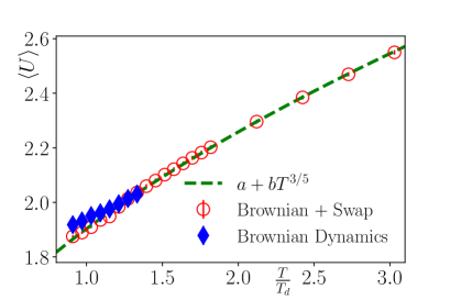
Figure 1: (Colour online) Potential energy $\langle U\rangle$ as a function of temperature for system size $N=10^{3}$. Blue diamonds refer to Brownian simulations, red circles refer to hybrid Brownian/Swap simulations. The dashed green line is the best fit to Rosenfeld and Tarazona formula [27]. $T_{\text{d}}$ is the dynamical temperature. Blue symbols deviate from Rosenfeld and Tarazona formula indicating that the corresponding stationary values of internal energy refer to configurations that are not well thermalized.

2.2 Inherent Structures and Density of States

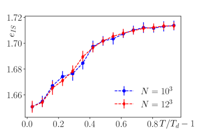
Figure 2: (Colour online) Average energy of the Inherent Structures $e_{\text{IS}}$ as the parental temperature $T$ changes for two system size, i.e., $N=10^{3}$ (blue symbols) and $N=12^{3}$ (red symbols).

After thermalization, we compute the corresponding inherent structures through the Limited-memory Broyden-Fletcher-Goldfarb-Shanno algorithm [29]. Let ${\mathbf{r}}$ be a configuration of the system, i.e., ${\mathbf{r}}\equiv({\mathbf{r}}_{1},\ldots,{\mathbf{r}}_{N})$. The mechanical energy of the configuration ${\mathbf{r}}$ is $E[{\mathbf{r}}]=\sum_{i<j}\phi(r_{ij})$. We indicate with ${\mathbf{r}}^{0}\equiv({\mathbf{r}}_{1}^{0},\ldots,{\mathbf{r}}_{N}^{0})$ the configuration that minimizes $E[{\mathbf{r}}]$, We define the Inherent Structure energy $e_{\text{IS}}\equiv N^{-1}\langle E[{\mathbf{r}}^{0}]\rangle_{s}$, with $\langle\dots\rangle_{s}$ indicating the average over $s$ independent configurations. The temperature dependence of $e_{\text{IS}}$ is shown in figure 2.

The spectrum of the harmonic oscillations around ${\mathbf{r}}^{0}$ is then obtained considering a perturbed configuration ${\mathbf{r}}={\mathbf{r}}^{0}+\bm{\delta r}$. The mechanical energy now reads $E[\bm{\delta r}]=E[{\mathbf{r}}^{0}]+\Delta E$ with $\Delta E\equiv\frac{1}{2}\sum_{i,j}\sum_{\mu\nu}\delta r_{i}^{\mu}M_{ij}^{\mu\nu}\delta r_{j}^{\nu}$ with $M_{ij}^{\mu\nu}$ the elements Hessian matrix $\mathbf{M}$, where Latin indices $i,j=1,\ldots,N$ indicate the particles and Greek symbols $\nu,\mu=1,\ldots,3$ the Cartesian coordinates. To estimate the correlation length $\xi$, we also considered configurations where a finite number of particles $pN$, with $p\in[0,1[$ the particle fraction, are maintained frozen during the minimization of $E[{\mathbf{r}}]$. The details about the minimization of $E[{\mathbf{r}}]$ with pinned particles can be found in reference [12]. We have computed all the $3N$ eigenvalues $\lambda_{\kappa}$, with $\kappa=1,\ldots,3N$, using gsl-GNU libraries for sizes up to $N=12^{3}$. The corresponding eigenvalues of $\mathbf{M}$ are $\omega_{\kappa}^{2}=\lambda_{\kappa}$.

To identify the low-frequency spectrum, we focus our attention on the cumulative $F(\omega)$=$\int_{0}^{\omega}\mathrm{d}\omega^{\prime}\,D(\omega^{\prime})$, where $D(\omega)$=$\mathcal{N}^{-1}\sum_{\kappa}\delta(\omega-\omega_{\kappa})$ is the density of states. $\mathcal{N}$ is the number of non-zero modes that is $3N-3$ for translational invariant systems.

The localization properties of the normal-modes have been investigated through the inverse participation ratio ${{\color[rgb]{0,0,0}\mathcal{R}}}(\omega)$ defined as ${{\color[rgb]{0,0,0}\mathcal{R}}}(\omega)\equiv\sum_{i}|{\mathbf{e}}_{i}(\omega)|^{4}/\left(\sum_{i}|{\mathbf{e}}_{i}(\omega)|^{2}\right)^{2}$ where ${\mathbf{e}}_{i}(\omega)$ is the eigenvector of the mode $\omega$ [30]. For a mode $\omega$ completely localized on a single particle, one has ${{\color[rgb]{0,0,0}\mathcal{R}}}(\omega)=1$, while a mode extended over all the particles corresponds to ${{\color[rgb]{0,0,0}\mathcal{R}}}(\omega)\sim N^{-1}$. We also compute $P(\mathcal{R})\equiv\mathcal{Q}\langle\sum_{\omega_{\lambda}:\omega_{\lambda}<\omega_{\text{th}}}\delta\left[\mathcal{R}(\omega_{\lambda})-\mathcal{R}\right]\rangle$ that is the probability distribution of the inverse participation ratio for the modes with frequency $\omega$ smaller than a threshold frequency $\omega_{\text{th}}$. $\mathcal{Q}$ is a normalization constant. After computing the distribution $P(\mathcal{R})$, we measure $\mathcal{R}_{a}\equiv\langle\log{\mathcal{R}}\rangle$.

3 Results

As it has been shown in reference [12], the non-Goldstone sector becomes clearly visible in $D(\omega)$, i.e., its weight in the density of states overcomes phonons, in systems with a finite fraction $p$ of frozen particles. In particular, non-Goldstone modes result to be soft, i.e., $D(\omega)\sim\omega^{s(p)}$ with $s(p)>2$ and localized, i.e., $\mathcal{R}(\omega)$ does not scale as $1/N$. These facts are in agreement with the soft potential model that predicts the scaling $D(\omega)\sim\omega^{4}$ for non-Goldstone excitations around the absolute minima in a one-dimensional random energy landscape [8]. Moreover, $D(\omega)$ at low frequencies changes its features when it is computed considering configurations thermalized with different protocols [23]. Thermalizing the system closer and closer to the dynamical transition, the corresponding inherent structures show the same type of crossover that can be described through a scaling $D(\omega)\sim\omega^{s(T)}$ [22]. Moreover, the same crossover can be documented through different observables, i.e., the effective exponent $s(T)$, the distribution of displacements travelled by particles for reaching the inherent structures, the mean-distance travelled by a particle for reaching the optimal configuration. Here, we focus our attention on the $\mathcal{R}$ of the low-frequency modes and their probability distribution function $P(\mathcal{R})$. We thus consider the inherent structures obtained starting from configurations thermalized at parental temperature $T$ that approaches the dynamical temperature $T_{\text{d}}$.

3.1 Localization of the glassy modes

In figure 3 we show the distribution $P(\mathcal{R})$ at temperature $T/T_{\text{d}}=1.42$ (blue) and $T/T_{\text{d}}=1.03$ (red). The distribution that has been computed considers only low-frequency modes. To do that, we impose a cutoff frequency $\omega_{\text{th}}$ that is chosen below the boson peak in the region where the power law scaling $D(\omega)\sim\omega^{s(T)}$ holds [22]. As one can appreciate, the distribution changes the shape and shifts towards higher $\mathcal{R}$ values as temperature decreases indicating that extended modes have been progressively suppressed.

To gain an insight into the role played by the cutoff frequency $\omega_{\text{th}}$, we have computed $P(\mathcal{R})$ for different values of $\omega_{\text{th}}$. The cutoff $\omega_{\text{th}}$ is taken below the frequency of the boson peak $\omega_{\text{BP}}$ which, in our models, is around $\omega_{\text{BP}}\sim 0.1$. The location of the boson peak in three spatial dimensions can be obtained looking at the maximum of $D(\omega)/\omega^{2}$ as shown, for instance, in reference [31]. We thus choose $\omega_{\text{th}}\in[0.02,0.1]$. The results are shown in figure 4 (a) in the case of $T/T_{\text{d}}=1.16$. The presence of extended modes at frequencies larger than $0.04$ dramatically changes the shape of $P(\mathcal{R})$. This is made evident when one looks at $\mathcal{R}_{a}$ as a function of temperature as it is shown in figure 4 (b). Choosing $\omega_{\text{th}}$ in the low-frequency region, i.e., $\omega_{\text{th}}<0.08$, $\mathcal{R}_{a}$ undergoes a smooth crossover as temperature decreases towards $T_{\text{d}}$. In particular, data for $\omega_{\text{th}}=0.02,0.03$ (blue symbols), i.e., a frequency that is below the boson peak, show that $\mathcal{R}_{a}$ starts to increase for $T/T_{\text{d}}-1<0.5$.

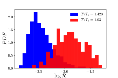
Figure 3: (Colour online) Probability distribution $P(\mathcal{R})$ at temperatures $T/T_{\text{d}}=1.42$ (blue) and $T/T_{\text{d}}=1.03$ (red). The cutoff frequency is $\omega_{\text{th}}=0.03$. As temperature decreases, the distribution shifts at higher $\mathcal{R}$ values.

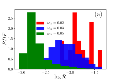
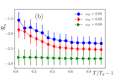
Figure 4: (Colour online) (a) $P(\mathcal{R})$ as $\omega_{\text{th}}$ increases from $0.02$ (red) to $0.05$ (green) and $T/T_{\text{d}}-1=0.24$. (b) $\mathcal{R}_{a}$ as a function of the parental temperature for different choices of $\omega_{\text{th}}$.

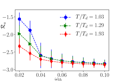
Figure 5: (Colour online) $\mathcal{R}_{a}$ ad a function of the threshold frequency $\omega_{\text{th}}$ at increasing temperature values ($T/T_{\text{d}}=1.03,1.29,1.23$, red, green, and blue symbols, respectively).

This finding is confirmed in figure 5 where we plot $\mathcal{R}_{a}$ as a function of $\omega_{\text{th}}$ for different values of $T/T_{\text{d}}=1.03,1.29,1.93$ (blue, green, and red symbols, respectively). We observe a region that is independent of both, $\omega_{\text{th}}$ and parental temperature $T$. Below $\omega_{\text{th}}\sim 0.05$, $\mathcal{R}_{a}$ increases as $\omega_{\text{th}}$ decreases but also as $T$ decreases. This is a clear signal that in the low-frequency region extended modes become attenuated in configurations thermalized at lower parental temperatures. It is worth noting that the behavior of $\mathcal{R}_{a}$ as a function of $T$ mirrors the behavior of $s(T)$ as shown in figure6 (b) where green symbols are $s(T)+1$ obtained from the cumulative distribution $F(\omega)$ [22].

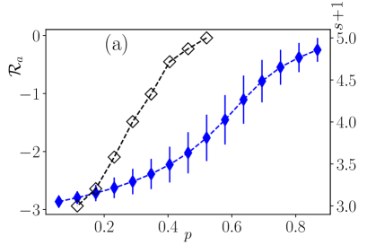
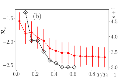
Figure 6: (Colour online) (a) $\mathcal{R}_{a}$ as a function of the fraction of pinned particles $p$ for configurations thermalized at high parental temperatures $T=0.5$. Open diamonds are the slope $s(p)$ of the power law $D(\omega)\sim\omega^{s(p)}$. (b) $\mathcal{R}_{a}$ as the parental temperature decreases and $p=0$. Solid symbols are $\mathcal{R}_{a}$, open diamonds the slope $s(T)$ of the power law $D(\omega)\sim\omega^{s(T)}$.

3.2 Comparison between $(T,p=0)$ and $(T=\infty,p)$ protocol

Now we are going to compare the localization properties of the eigemodes obtained at high parental temperatures but considering a finite fraction of a frozen particle during the minimization of the mechanical energy with those obtained in the non-pinned system as a function of $T$. It has been shown that, as $p$ increases, $D(\omega)\sim\omega^{s(p)}$ with $s(p)$ undergoing a smooth crossover from $s=2$ to $s=4$ above a threshold value $p_{\text{th}}\sim 0.5$ [12]. We refer to this protocol as $(T=\infty,p)$, since one considers configuration thermalized at high temperatures, i.e., away from $T_{\text{d}}$. In the previous section, we have considered a protocol where the inherent structures were computed considering configutations thermalized at parental temperatures $T$ close to $T_{\text{d}}$. We refer to this protocol as $(T,p=0)$ since energy minimization has been computed without any artificially frozen particle.

Also in the case of the pinned system, modes responsible for $\omega^{4}$ are localized. This is because they live in between the frozen regions induced by the random pinning protocol. Since the number of frozen particle increases, the lowest frequency of the spectrum naturally shifts towards higher values and the threshold value $\omega_{\text{th}}$ as well. Random pinning explicitly destroys the translational invariance removing the corresponding three zero modes from the spectrum and attenuating any extended mode. This has a strong effect on $\mathcal{R}_{a}$ that grows towards $\mathcal{R}_{a}\sim 0$ for $p\to 1$, as it is shown in figure 6 (a), blue symbols. Also in this case, similarly to what we observed in the previous protocol, i.e., decreasing the parental temperature without any artificially frozen particle, $\mathcal{R}_{a}$ undergoes a crossover mirroring that in $s(p)$ (black symbols in the same panel). It is worth noting that in both protocols when the density of states undergoes a crossover $s\to 4$, $R_{a}\sim-1.5$.

Since frozen particles occupy a finite volume fraction $pV$, we can associate to the volume fraction a typical length scale $\xi{\color[rgb]{0,0,0}\equiv(pV)^{1/3}}$. In reference [22] it has been shown that, looking at the solution of $s(p,T=\infty)=s(T,p=0)$, one can extract the behavior of $\xi^{3}$ as a function of the parental temperature $T$. Here, we can extract $\xi^{3}$ looking at the degree of localization of the low-frequency modes. To do that, we solve and invert numerically $\mathcal{R}_{a}(T,p=0)-\mathcal{R}_{a}(T=\infty,p=0)=\mathcal{R}_{a}(T=\infty,p)-\mathcal{R}_{a}(T=\infty,p=0.1)$. The result is shown in figure 7, red symbols. Green symbols refer to the solution of $s(p,T=\infty)=s(T,p=0)$. As one can see, the two data sets are in a good agreement.

4 Conclusions

In this paper, we have investigated the localization properties of low-frequency modes in a three-dimensional model of supercooled liquid. In particular, we have focused our attention on the role played by the parental temperature on the localization of the soft glassy modes. Our findings show that low-frequency vibrational modes at lower parental temperature turn out to be more localized than those populating the density of states at higher $T$ values. This is consistent with the results presented in [22, 23] and also with simulations on well-equilibrated polydisperse glass former [13]. In particular, the increasing in localization takes place near the dynamical transition temperature $T_{\text{d}}$ that is where the exponent $s(T)$ of the power law $D(\omega)\sim\omega^{s(T)}$ approaches $s(T_{\text{d}})\to 4$. This finding confirms the interplay between dynamical and zero-temperature structural properties in glasses [22]. At lower temperatures, we also observed a dependency of $\mathcal{R}_{a}$ on the cutoff frequency $\omega_{\text{th}}$. This shift reminds the effect of random pinning on the density of states [12].

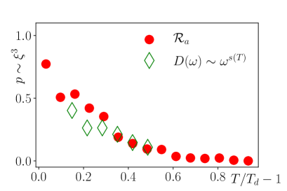
Figure 7: (Colour online) Comparison between the typical length scale $\xi^{3}$ computed in reference [22] (open diamonds) with an estimate of $\xi^{3}$ based on $\mathcal{R}_{a}$ (solid circles).

We have thus investigated how the localization of the lowest eigenmodes takes place in the same system with random pinning. In particular, we observed that the same scenario of progressive localization of glassy modes takes place as the number of frozen particles increases. In the pinning protocol, the emergence of soft localized excitations is due to the breaking of translational invariance in the system. With increasing $p$, moving particles rattle into small islands that are surrounded by the frozen ones. At higher values, i.e., for $p>p_{\text{th}}$, the phononic spectrum is totally destroyed giving rise to extremely localized modes, i.e., $\mathcal{R}\to 1$. This marks a difference with a system thermalized at lower parental temperatures where the translational invariance is preserved. Nevertheless, configurations thermalized at lower temperatures show a spectrum of harmonic vibrations whose properties are remarkably similar to those obtained breaking explicitly the spatial translational invariance, i. e., crossover in $D(\omega)$ from Debye to non-Debye, localization of low-frequency modes, caging effects during minimization. We can thus extract useful and complementary information comparing the region $p<p_{\text{th}}$, in the $(T=\infty,p)$ protocol, with $T>T_{\text{d}}$, in the $(T,p=0)$ protocol. In this paper, we provide evidences for a crossover from extended to localized modes at low-frequencies as temperature decreases towards $T_{\text{d}}$ which is in agreement with recent works [13, 32]. We also showed that, in analogy with reference [22], $\mathcal{R}_{a}$ can be employed for mapping structural properties into dynamical ones. In particular, the degree of localization measured through $\mathcal{R}_{a}$ is regulated by the proliferation of dynamical heterogeneous regions in the $(T,p=0)$ protocol. The $(T=\infty,p)$ protocol allows one to define a length scale $\xi\sim p^{1/3}$ that is an external and tunable parameter. We can thus study $p=p(T)$ just looking at the solution of $\mathcal{O}(T,p=0)=\mathcal{O}(T=\infty,p)$, with $\mathcal{O}$ being a generic observable. As it has been shown in reference [22], $p(T)$ mirrors the behavior of the dynamical length scale $\xi_{\text{dyn}}$ [33]. Here, we showed that from $\mathcal{R}_{a}$ we can extract the behavior of $p(T)$ which is in agreement with those observed through other observables [22].

As a future direction, it would be interesting to study the density of states in systems thermalized at parental temperature $T$ close to $T_{\text{d}}$ with a fraction $p$ of pinned particles. In this way, in the spirit of early works on random pinning [14, 15, 16, 17, 18, 19, 20, 21], it would be possible to take access to the properties of glassy modes towards the Kauzmann temperature.

Ukrainian 0

Íèçüêîчàñòîòíi çáóäæåííÿ òà âëàñòèâîñòi ¿õ ëîêàëiçàöi¿ ó ñêëîâèäíèõ ñèñòåìàõ Ì. Ïàîëóööi${}^{\textsf{\footnotesize{\mbox{?}}}}$, Ë. Àíäæåëàíi${}^{\textsf{\footnotesize{\mbox{?},\penalty 1000\mbox{?}}}}$

             
${}^{\textsf{\footnotesize 1}}$ Ôiçèчíèé ôàêóëüòåò, Ðèìñüêèé óíiâåðñèòåò ‘‘Sapienza’’, ïë. A. Moðî, 2, I-00185 Ðèì, Iòàëiÿ ${}^{\textsf{\footnotesize 2}}$ ISC-CNR, Iíñòèòóò ñêëàäíèõ ñèñòåì, ïë. A. Moðî, 2, I-00185 Ðèì, Iòàëiÿ

References

- [1] Binder K., Kob W., Glassy Materials and Disordered Solids: An Introduction to Their Statistical Mechanics, World Scientific, Singapore, 2011, doi:10.1142/7300.
- [2] Leuzzi L., Nieuwenhuizen T.M., Thermodynamics of the Glassy State, CRC Press, New York, 2007.
- [3] Berthier L., Biroli G., Rev. Mod. Phys., 2011, 83, 587–645, doi:10.1103/RevModPhys.83.587.
- [4] Debenedetti P.G., Stillinger F.H., Nature, 2001, 410, 259–267, doi:10.1038/35065704.
- [5] Cavagna A., Phys. Rep., 2009, 476, 51–124, doi:10.1016/j.physrep.2009.03.003.
- [6] Kittel C., Introduction to Solid State Physics, Wiley & Sons, New York, 2005.
- [7] Zeller R.C., Pohl R.O., Phys. Rev. B, 1971, 4, 2029–2041, doi:10.1103/PhysRevB.4.2029.
- [8] Gurarie V., Chalker J.T., Phys. Rev. B, 2003, 68, 134207, doi:10.1103/PhysRevB.68.134207.
-
[9]
Baity-Jesi M., Martín-Mayor V., Parisi G., Perez-Gaviro S., Phys. Rev.
Lett., 2015, 115, 267205,
doi:10.1103/PhysRevLett.115.267205. -
[10]
Lerner E., Düring G., Bouchbinder E., Phys. Rev. Lett., 2016, 117,
035501,
doi:10.1103/PhysRevLett.117.035501. -
[11]
Mizuno H., Shiba H., Ikeda A., Proc. Natl. Acad. Sci. U.S.A.,
2017, 114, E9767–E9774,
doi:10.1073/pnas.1709015114. -
[12]
Angelani L., Paoluzzi M., Parisi G., Ruocco G., Proc. Natl. Acad. Sci. U.S.A., 2018, 115, 8700–8704,
doi:10.1073/pnas.1805024115. -
[13]
Wang L., Ninarello A., Guan P., Berthier L., Szamel G., Flenner E., Nat. Commun., 2019, 10, 26,
doi:10.1038/s41467-018-07978-1. - [14] Cammarota C., Biroli G., J. Chem. Phys., 2013, 138, 12A547, doi:10.1063/1.4790400.
- [15] Cammarota C., Biroli G., Proc. Natl. Acad. Sci. U.S.A., 2012, 109, 8850–8855, doi:10.1073/pnas.1111582109.
- [16] Szamel G., Flenner E., Europhys. Lett., 2013, 101, 66005, doi:10.1209/0295-5075/101/66005.
- [17] Kob W., Roldán-Vargas S., Berthier L., Nat. Phys., 2012, 8, 164, doi:10.1038/nphys2133.
-
[18]
Gokhale S., Nagamanasa K.H., Ganapathy R., Sood A., Nat. Commun.,
2014, 5, 4685,
doi:10.1038/ncomms5685. - [19] Karmakar S., Parisi G., Proc. Natl. Acad. Sci. U.S.A., 2013, 110, 2752–2757, doi:10.1073/pnas.1222848110.
- [20] Kob W., Berthier L., Phys. Rev. Lett., 2013, 110, 245702, doi:10.1103/PhysRevLett.110.245702.
-
[21]
Ozawa M., Kob W., Ikeda A., Miyazaki K., Proc. Natl. Acad. Sci. U.S.A., 2015, 112, 6914–6919,
doi:10.1073/pnas.1500730112. -
[22]
Paoluzzi M., Angelani L., Parisi G., Ruocco G., Phys. Rev. Lett., 2019, 123, 155502,
doi:10.1103/PhysRevLett.123.155502. - [23] Lerner E., Bouchbinder E., Phys. Rev. E, 2017, 96, 020104(R), doi:10.1103/PhysRevE.96.020104.
-
[24]
Kob W., Donati C., Plimpton S.J., Poole P.H., Glotzer S.C., Phys. Rev. Lett.,
1997, 79, 2827–2830,
doi:10.1103/PhysRevLett.79.2827. -
[25]
Bernu B., Hansen J.P., Hiwatari Y., Pastore G., Phys. Rev. A, 1987,
36, 4891–4903,
doi:10.1103/PhysRevA.36.4891. - [26] Grigera T.S., Parisi G., Phys. Rev. E, 2001, 63, 045102, doi:10.1103/PhysRevE.63.045102.
- [27] Rosenfeld Y., Tarazona P., Mol. Phys., 1998, 95, 141–150, doi:10.1080/00268979809483145.
-
[28]
Lacevic N., Starr F.W., Schroder T.B., Glotzer S.C., J. Chem.
Phys., 2003, 119, 7372–7387,
doi:10.1063/1.1605094. - [29] Bonnans J.F., Gilbert J.C., Lemaréchal C., Sagastizábal C.A., Numerical Optimization: Theoretical and Practical Aspects, Springer Science & Business Media, 2006.
- [30] Bell R., Dean P., Spec. Discuss. Faraday Soc. Special, 1970, 50, 55–61, doi:10.1039/DF9705000055.
- [31] Grigera T., Martín-Mayor V., Parisi G., Verrocchio P., Nature, 2003, 422, 289, doi:10.1038/nature01475.
- [32] Coslovich D., Ninarello A., Berthier L., Preprint arXiv:1811.03171, 2018.
-
[33]
Biroli G., Bouchaud J.-P., Miyazaki K., Reichman D.R., Phys. Rev. Lett., 2006,
97, 195701,
doi:10.1103/PhysRevLett.97.195701.
Ukrainian \adddialect\l@ukrainian0 \l@ukrainian