Chiral Effective Field Theory Description of Neutrino Nucleon-Nucleon Bremsstrahlung in Supernova Matter

Abstract

We revisit the rates of neutrino pair emission and absorption from nucleon-nucleon bremsstrahlung in supernova matter using the $T$-matrix formalism in the long-wavelength limit. Based on two-body potentials of chiral effective field theory ($\chi$EFT), we solve the Lippmann-Schwinger equation for the $T$-matrix including non-diagonal contributions. We consider final-state Pauli blocking and hence our calculations are valid for nucleons with an arbitrary degree of degeneracy. We also explore the in-medium effects on the $T$-matrix and find that they are relatively small for supernova matter. We compare our results with one-pion exchange rates, commonly used in supernova simulations, and calculations using an effective on-shell diagonal $T$-matrix from measured phase shifts. We estimate that multiple-scattering effects and correlations due to the random phase approximation introduce small corrections on top of the $T$-matrix results at subsaturation densities. A numerical table of the structure function is provided that can be used in supernova simulations.

1 Introduction

Neutrino interaction with nucleons in proto-neutron stars (PNS) (Burrows et al., 2006) plays a crucial role in many aspects of core-collapse supernovae (CCSNe), such as the explosion mechanism (Burrows, 2013; Janka et al., 2007; Janka, 2012) as well as the synthesis of heavy elements in neutrino-driven winds (Arcones & Thielemann, 2013; Martínez-Pinedo et al., 2016) and the long-term cooling of the neutron star (Yakovlev et al., 2001; Yakovlev & Pethick, 2004). Three-dimentional (3D) simulations with detailed neutrino transport have shown that explosions are very sensitive to neutrino opacities even at the level of 10%–20% (Melson et al., 2015; Burrows et al., 2018). Therefore, an accurate description of neutrino interaction in hot and dense nuclear matter related to CCSNe is highly demanded.

We revisit the neutrino pair emission and absorption from NN collision in supernova (SN) matter using $T$-matrix elements based on $\chi$EFT potentials following Bartl et al. (2014); Bartl (2016). Neutrino bremsstrahlung $NN\to NN\nu\bar{\nu}$, its inverse $NN\nu\bar{\nu}\to NN$, and the related inelastic scattering $NN\nu\to NN\nu$ play key roles in changing the number density and energy for the heavy-flavor SN neutrinos and are thus important in determining the neutrino spectra formation (Raffelt, 2001; Keil et al., 2003). The most widely used bremsstrahlung rate in SN simulations (Hannestad & Raffelt, 1998) is based on the one-pion exchange (OPE) potential in the Born approximation with only interactions among neutrons considered. As already mentioned by Hannestad & Raffelt (1998), a proper treatment of NN correlations for general nuclear matter should be considered for a better description of neutrino bremsstrahlung (see also Friman & Maxwell, 1979; Sigl, 1997; Yakovlev et al., 2001; Bartl et al., 2014; Pastore et al., 2015; Dehghan Niri et al., 2016, 2018; Riz et al., 2018). Modern nuclear interactions from $\chi$EFT have been used to study neutrino bremsstrahlung based on the Landau’s theory of Fermi liquids (Lykasov et al., 2008; Bacca et al., 2009, 2012; Bartl et al., 2014; Bartl, 2016). The necessity to go beyond the Born approximation was demonstrated by Bartl et al. (2014) using effective on-shell $T$-matrix elements extracted from experimental phase shifts (see also Sigl, 1997; Hanhart et al., 2001; van Dalen et al., 2003). It should be pointed out (Bartl et al., 2014), however, that the use of the on-shell $T$-matrix is only valid in the limit of zero energy transfer between nucleons and the neutrino pair. For finite energy transfer, off-shell $T$-matrix elements are needed. van Dalen et al. (2003) also explored the in-medium effects on the $T$-matrix based on the Bonn C potential for neutrino bremsstrahlung rates, but their study was limited to neutrino emissivities in conditions relevant to neutron stars. Bartl et al. (2014) performed the first calculation of NN bremsstrahlung for arbitrary mixtures of neutrons and protons in supernova matter.

In this work we aim for an improved description of neutrino bremsstrahlung that includes both off-shell matrix elements and Pauli blocking effects. We solve the Lippmann-Schwinger (LS) equation to obtain the vacuum $T$-matrix (Lippmann & Schwinger, 1950) and the Bethe-Goldstone (BG) equation (Bethe, 1956; Goldstone, 1957) to account for in-medium effects in the $T$-matrix. The bremsstrahlung rate, or more precisely the associated structure function $S(q,\omega)$, with $q$ and $\omega$ the momentum and energy transfer, is obtained using the Fermi’s golden rule in the long wavelength limit ($q\to 0$), which is consistent with that derived from the finite-temperature linear response theory (see, e.g., Weldon, 1983; Roberts & Reddy, 2017). To account for multiple-scattering effects and to get around of divergences at $\omega\to 0$, we introduce a relaxation rate parameter or width parameter whose value is determined from the normalization of $S(q\to 0,\omega)$ (Hannestad & Raffelt, 1998). Our calculations consider final-state blocking for the nucleons in calculating the bremsstrahlung rates. They are compared to results using Boltzmann distributions without blocking, which are only valid in the non-degenerate regions.

The paper is organized as follows. In Sec. 2, we calculate perturbatively the structure function and the neutrino bremsstrahlung rate, and then study the effects of using different nuclear matrix elements (vacuum $T$-matrix, in-medium $T$-matrix and OPE potential) with/without blocking, and with half-off-shell or on-shell matrix elements. In Sec. 3, we include the width parameter to normalise the structure function properly, and then compare our results with the previous ones in the literature. Correlation effects due to the random phase approximation (RPA) are considered and studied in Sec. 4. We present a summary and discussions in Sec. 5.

2 Neutrino bremsstrahlung rate: perturbative calculation

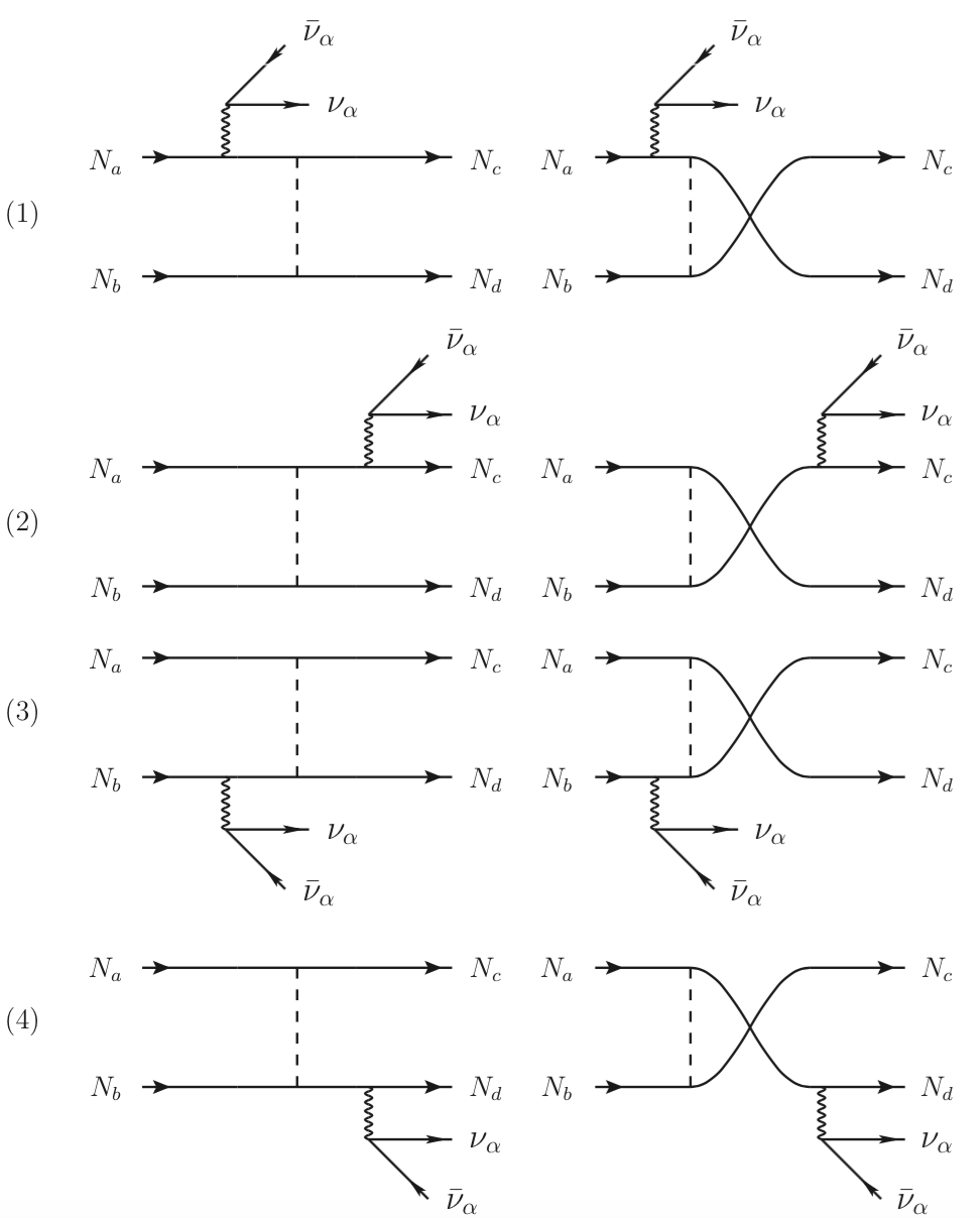
Figure 1: Feynman diagrams of neutrino bremsstrahlung, $N_{a}+N_{b}\to N_{c}+N_{d}+\nu_{\alpha}+\bar{\nu}_{\alpha}$, where $N$ stands for either a neutron, $n$, or a proton, $p$, and $\alpha=e,\mu,\tau$ for different neutrino flavors. Both the direct (left) and exchange (right) diagrams are considered.

2.1 Formalism

To study neutrino bremsstrahlung and related processes, we consider the diagrams as shown in Figure 1, including both the direct and the exchange contributions. Neglecting weak magnetism and pseudoscalar corrections, the amplitudes of the diagrams are

$$M^{(1)} =\frac{G_{F}C^{a}_{A}}{\sqrt{2}}\,{}_{\text{nas}}\langle cd|V\bm{\sigma}^{(a)}_{i}|ab\rangle_{\text{nas}}\,\frac{l_{i}}{\omega},$$ (1a)

$$M^{(2)} =-\frac{G_{F}C^{c}_{A}}{\sqrt{2}}\,{}_{\text{nas}}\langle cd|\bm{\sigma}^{(c)}_{i}V|ab\rangle_{\text{nas}}\,\frac{l_{i}}{\omega},$$ (1b)

$$M^{(3)} =\frac{G_{F}C^{b}_{A}}{\sqrt{2}}\,{}_{\text{nas}}\langle cd|V\bm{\sigma}^{(b)}_{i}|ab\rangle_{\text{nas}}\,\frac{l_{i}}{\omega},$$ (1c)

$$M^{(4)} =-\frac{G_{F}C^{d}_{A}}{\sqrt{2}}\,{}_{\text{nas}}\langle cd|\bm{\sigma}^{(d)}_{i}V|ab\rangle_{\text{nas}}\,\frac{l_{i}}{\omega},$$ (1d)

where $|ab\rangle_{\text{nas}}$ and $|cd\rangle_{\text{nas}}$ are normalized antisymmetric states of the initial and final nucleon pair, which are characterized by their relative momenta and spin projections (see Appendix B for more details). For neutrino pair absorption we have $\omega=(E_{\nu}+E_{\bar{\nu}})>0$. $\bm{\sigma}_{i}^{(a)}$ ($i=x,y,z$) are the Pauli matrices acting on the nucleon $N_{a}$, $l_{i}$ are the spatial components of the leptonic weak current, $C^{a}_{A}=g_{A}/2\simeq 0.63$ if $N_{a}$ is a proton and $C_{A}^{a}=-g_{A}/2$ if it is a neutron, and $G_{F}$ is the Fermi coupling constant. Note that we do not include the vector terms in ${\cal M}^{(1,2,3,4)}$ since they cancel each other out in the non-relativistic limit within the Born approximation (Friman & Maxwell, 1979; Raffelt & Seckel, 1995; Hannestad & Raffelt, 1998). Going beyond the Born approximation and using the half-off-shell $T$-matrix, the complete cancellation of the vector terms does not hold any longer. Nevertheless, its contribution is negligible compared to the axial-vector terms. $V$ could denote either the nucleon-nucleon scattering $T$-matrix based on the $\chi$EFT potential of Entem et al. (2017) with cutoff $\Lambda=500$ MeV or the OPE potential. For comparison with previous results (Friman & Maxwell, 1979; Hannestad & Raffelt, 1998; Bartl et al., 2014), the OPE potential is treated in the Born approximation. In the limit of non-degenerate nucleons our OPE results are identical to those of Bartl et al. (2014). We will use $\mathcal{T}$ to explicitly denote the scattering $T$-matrix based on the $\chi$EFT potential. Bartl et al. (2014) have shown, that in the Born approximation, OPE and $\chi$EFT potentials give similar rates at subsaturation densities as they are dominated by the long-range part of the tensor force, that is well described by the OPE potential. However, they also showed that the low-energy resonant nature of the nucleon-nucleon interaction (Bartl et al., 2014) enhances the rates and requires one to go beyond the Born approximation.

The total amplitude can be written in a more compact form as

$$\mathcal{M}_{\text{tot}}= \sum_{j=1}^{4}M^{(j)}=-\frac{G_{F}g_{A}}{2\sqrt{2}\omega}$$ (2)

$$\times{}_{\text{nas}}\langle cd|[V,\sum_{r}\bm{\sigma}^{(r)}_{i}\bm{\tau}_{z}^{(r)}]^{\prime}|ab\rangle_{\text{nas}}\,l_{i},$$

where $\bm{\tau}_{z}$ is the $z$-component of the isospin operator with $\bm{\tau}_{z}|n\rangle=|n\rangle$ and $\bm{\tau}_{z}|p\rangle=-|p\rangle$, and $r$ runs over the two initial or final nucleons. The prime in the commutator denotes that the potential is evaluated at different values of the energy for the first (“positive”) and second (“negative”) terms; see the definition in Equation (B20). For energy-independent potentials, such as the OPE or the chiral potential at the Born level, it reduces to the standard commutator. The squared amplitude can be divided into leptonic, $L$, and hadronic, $H$, parts as $\sum_{\text{spins}}|\mathcal{M}_{\text{tot}}|^{2}=(G_{F}^{2}g^{2}_{A}/8)\sum_{ij}H_{ij}L^{ij}$. For an isotropic medium, we only need to consider the trace average of the hadronic part (Hannestad & Raffelt, 1998):

$$\sum_{\text{spins}} |\mathcal{M}_{\text{tot}}|^{2}\xrightarrow{\text{isotropic}}G_{F}^{2}g^{2}_{A}\bar{H}E_{\nu}E_{\nu^{\prime}}(3-\cos\theta_{\nu\nu^{\prime}}),$$ (3)

$$\bar{H} \equiv\frac{1}{3}\sum_{i}H_{ii}$$

$$=\frac{1}{3}\sum_{i}\sum_{\text{spins}}|{}_{\text{nas}}\langle cd|[V,\frac{1}{\omega}\sum_{r=1,2}\bm{\sigma}^{(r)}_{i}\bm{\tau}_{z}^{(r)}]^{\prime}|ab\rangle_{\text{nas}}|^{2}.$$

Note that $\bar{H}$ is a scalar under rotations due to the invariance of the trace under basis transformations. The partial wave expansions of $\bar{H}^{(nn)}=\bar{H}^{(pp)}$ and $\bar{H}^{(np)}=\bar{H}^{(pn)}$ are presented in Appendix B. The calculation of $\bar{H}$ requires the evaluation of the $T$-matrix elements in momentum space $\langle\bm{k}_{f}|\mathcal{T}|\bm{k}_{i}\rangle$, where $\bm{k}_{i}\equiv(\bm{k}_{a}-\bm{k}_{b})/2$ and $\bm{k}_{f}\equiv(\bm{k}_{c}-\bm{k}_{d})/2$ are the relative momenta of the initial and final nucleon pair, and only the initial or final nucleon pair is on-shell for finite values of $\omega$ (see Figure. 1), i.e., we deal with half-off-shell matrix elements. Here, we fully consider their contribution when we solve the Lippmann-Schwinger equation based on the $\chi$EFT potential of Entem et al. (2017). Additionally, we include in-medium Pauli blocking effects (see Appendix A) when solving the Bethe-Goldstone equation. With such medium effects taken into account, $\bar{H}$ is a function of $K=|\bm{K}|\equiv|\bm{k}_{a}+\bm{k}_{b}|=|\bm{k}_{c}+\bm{k}_{d}|$, $k_{i}=|\bm{k}_{i}|$, $k_{f}=|\bm{k}_{f}|$, and $\cos\theta$, where $\theta$ is the angle between $\bm{k}_{i}$ and $\bm{k}_{f}$.

The response of a nuclear medium can be described by the so-called structure function or response function. For neutrino bremsstrahlung in the long-wavelength limit (i.e., we ignore momentum exchange), the axial structure function, $S^{(\lambda\eta)}_{\sigma}$, with $\lambda,\eta=n$ or $p$, is given by (Hannestad & Raffelt, 1998; Lykasov et al., 2008; Bartl et al., 2014)

$$S_{\sigma}^{(\lambda\eta)}(\omega)= {1\over n_{B}}\int\Biggl{(}\prod_{l=a,b,c,d}\frac{d^{3}k_{l}}{(2\pi)^{3}}\Biggr{)}f_{a}f_{b}(1-f_{c})(1-f_{d})$$ (4)

$$\times \delta^{(3)}(\bm{k}_{a}+\bm{k}_{b}-\bm{k}_{c}-\bm{k}_{d})\bar{H}^{(\lambda\eta)}(K,k_{i},k_{f},\cos\theta)$$

$$\times (2\pi)^{4}\delta(E_{a}+E_{b}-E_{c}-E_{d}+\omega),$$

where $n_{B}$ is the total baryon number density and $f_{l}$ are the Fermi functions. Throughout this work, we always take the non-relativistic energy-momentum relation, and correspondingly the non-relativistic chemical potential without including the rest mass. Note that, unlike the formalisms adopted in Hannestad & Raffelt (1998), we do not need to consider a symmetry factor for identical nucleon species since our matrix element is calculated for normalised antisymmetric nucleon states. In the perturbative limit of Equation (4) the total axial structure function, $S_{\sigma}$, is simply

$$S_{\sigma}(\omega)=S^{(nn)}_{\sigma}(\omega)+S^{(pp)}_{\sigma}(\omega)+S^{(np)}_{\sigma}(\omega).$$ (5)

The structure function in Equation (4) with the Fermi distributions and blocking involves a multidimensional integral, which can only be computed numerically. We choose $\bm{k}_{i}$ along the $z$-axis, and without loss of generality we set $\bm{k}_{a}$ in the $xz$-plane with a polar angle denoted by $\theta_{a}$. We further denote the polar and the azimuthal angles of $\bm{k}_{f}$ by $\theta$ and $\phi$. Once $k_{i}$, $k_{a}$, $\theta$, $\phi$, and $\theta_{a}$ are specified, all momenta are then fixed, making Equation (4) a five-dimensional integral. We use the Vegas subroutine in the CUBA library (Hahn, 2005), invoking a Monte Carlo algorithm to evaluate all the multidimensional integrals in this work.

In the non-degenerate limit, we have $f_{a}f_{b}(1-f_{c})(1-f_{d})\simeq f_{a}f_{b}\simeq\exp\{[(-K^{2}/4-k_{i}^{2})/m_{N}+\mu_{a}+\mu_{b}]/T\}$, independent of all the angles, and $S_{\sigma}(\omega)$ can be simplified to

$$S^{(\lambda\eta)}_{\sigma,m,b}(\omega)= {4m_{N}\over(2\pi)^{5}n_{B}}\int dKdk_{i}K^{2}k_{i}^{2}k_{f}\bar{H}^{(\lambda\eta)}_{L=0}(K,k_{i},k_{f})$$ (6)

$$\times\exp\left\{-\frac{K^{2}/(4m_{N})+k_{i}^{2}/m_{N}-\mu_{a}-\mu_{b}}{T}\right\},$$

where $m_{N}=(m_{n}+m_{p})/2$ is the averaged nucleon mass, and $\mu_{a,b}$ are the non-relativistic chemical potentials of nucleons. Since $\int d\cos\theta P_{L}(\cos\theta)=2\delta_{L0}$, where $P_{L}$ is the Legendre polynomial, only the $L=0$ component of $\bar{H}$ contributes; see Equation (B18). We use the subscript $m$ ($v$) to refer to the in-medium (vacuum) $T$-matrix elements, and $b$ ($f$) when we use the Boltzmann (Fermi) distribution without (with) blocking. Throughout this work, we always take the bare nucleon mass for all our studies. For typical densities in the neutrinosphere, the effective mass of nucleons is close to the bare value. At the saturation density, $\chi$EFT calculations (Hebeler et al., 2009; Wellenhofer et al., 2014; Drischler et al., 2017) found an effective mass $\sim 0.9\,m_{N}$. Using such a value for both proton and neutron, the rates are only affected by a few per cent.

When the vacuum $T$-matrix elements or the OPE potential are used, $\bar{H}^{(\lambda\eta)}$ is independent of $K$ and integration over $K$ can be done analytically with $\int dKK^{2}\exp(-K^{2}/(4m_{N}T))=\sqrt{4\pi(m_{N}T)^{3}}$, leading to

$$S^{(\lambda\eta)}_{\sigma,v,b}(\omega)= {(2m_{N})^{5/2}T^{3/2}\over(2\pi)^{9/2}n_{B}}\int dk_{i}k_{i}^{2}k_{f}\bar{H}^{(\lambda\eta)}_{L=0}(k_{i},k_{f})$$ (7)

$$\times\exp\left\{-\frac{k_{i}^{2}/m_{N}-\mu_{a}-\mu_{b}}{T}\right\}.$$

Once $S_{\sigma}(\omega)$ is known, the inverse mean free path or opacity of a neutrino against neutrino pair absorption is

$$\lambda^{-1}_{A}(E_{\nu})= \frac{g_{A}^{2}G_{F}^{2}n_{B}}{4}\int{d^{3}k^{\prime}\over(2\pi)^{3}}(3-\cos\theta_{\nu\bar{\nu}})f^{\prime}(E^{\prime}_{\nu})$$ (8)

$$\times S_{\sigma}(E_{\nu}+E^{\prime}_{\nu}),$$

where $\bm{k}^{\prime}$ and $f^{\prime}$ are the momentum and distribution function of the counterpart (anti)neutrino, and $\theta_{\nu\bar{\nu}}$ is the angle between the neutrino momenta.

The spectrum of emitted neutrinos with a particular flavor per unit of solid angle is

$$\phi(E_{\nu})= \frac{g_{A}^{2}G_{F}^{2}n_{B}E_{\nu}^{2}}{4(2\pi)^{3}}\int{d^{3}k^{\prime}\over(2\pi)^{3}}(3-\cos\theta_{\nu\bar{\nu}})$$ (9)

$$\times S_{\sigma}(-E_{\nu}-E_{\nu^{\prime}})[1-f(E_{\nu})][1-f^{\prime}(E_{\nu^{\prime}})].$$

If one can neglect the final-state blocking of neutrinos, Equation (9) can be further simplified to

$$\phi(E_{\nu})\approx\frac{3g_{A}^{2}G_{F}^{2}n_{B}E_{\nu}^{2}}{4(2\pi)^{3}} \int{4\pi E_{\nu^{\prime}}^{2}dE_{\nu^{\prime}}\over(2\pi)^{3}}S_{\sigma}(E_{\nu}+E_{\nu^{\prime}})$$ (10)

$$\times e^{-(E_{\nu}+E_{\nu^{\prime}})/T},$$

where we have used the detailed balanced relation $S_{\sigma}(-\omega)=S_{\sigma}(\omega)\exp(-\omega/T)$. Assuming thermal distributions for neutrinos, we find $\phi(E_{\nu})/\lambda_{A}^{-1}(E_{\nu})\propto E_{\nu}^{2}\exp(-E_{\nu}/T)$. For demonstration, we always use Equation (10) to calculate the neutrino spectra emitted, but the final-state neutrino blocking can be easily included in neutrino transport in realistic supernova simulations. Similarly, the energy loss rate due to neutrino pair emission is

$$Q_{\text{brem}}= \frac{3}{4}g_{A}^{2}G_{F}^{2}n_{B}\int{d^{3}k\over(2\pi)^{3}}{d^{3}k^{\prime}\over(2\pi)^{3}}(3-\cos\theta)(E_{\nu}+E^{\prime}_{\nu}),$$ (11)

which can be approximated by

$$Q_{\text{brem}}\approx \frac{3g_{A}^{2}G_{F}^{2}n_{B}}{160\pi^{4}}\int_{0}^{\infty}d\omega\omega^{6}e^{-\omega/T}S_{\sigma}(\omega),$$ (12)

if the final-state neutrino blocking can be neglected. Note that the prefactor 3 accounts for three different neutrino flavors.

Assuming the neutrino spectrum follows a Boltzmann distribution, $f(E_{\nu})\propto\exp(-E_{\nu}/T_{\nu})$, with a neutrino temperature $T_{\nu}=T$, the energy-averaged pair absorption inverse mean free path per neutrino can be expressed as

$$\frac{\langle\lambda^{-1}_{A}\rangle}{n_{\nu}^{\prime}}\equiv \frac{1}{n^{\prime}_{\nu}}\frac{\int\lambda_{A}^{-1}(E_{\nu})f(E_{\nu})E_{\nu}^{2}dE_{\nu}}{\int f(E_{\nu})E_{\nu}^{2}dE_{\nu}}$$ (13)

$$= \frac{g_{A}^{2}G_{F}^{2}n_{B}}{160T^{6}}\int_{0}^{\infty}d\omega\omega^{5}e^{-\omega/T}S_{\sigma}(\omega).$$

We use the inverse mean free path per neutrino number density instead of the inverse mean free path because the latter depends on the number density of neutrinos, which needs to be determined by full Boltzmann transport calculations.

2.2 Energy-averaged inverse mean free path using different treatments

As already mentioned above, we can perform calculations based on different schemes: vacuum $T$-matrix, in-medium $T$-matrix and OPE potential; each considers different approximations: either on-shell or half-off-shell and the Boltzmann or Fermi distribution that includes final-state blocking. In what follows, we firstly consider $\langle\lambda_{A}^{-1}\rangle/n_{\nu}^{\prime}$ based on the vacuum/in-medium $T$-matrix and the OPE potential, and explore the effects of the different approximations. As in Bartl et al. (2014), we take the typical conditions in SNe characterized by

$$T_{SN}(\rho)=3~{}\text{MeV}~{}\Big{(}{\rho\over 10^{11}~{}\text{g cm}^{-3}}\Big{)}^{1/3},$$ (14)

and choose $Y_{e}=0.1,0.3$, and 0.5 for the following studies.

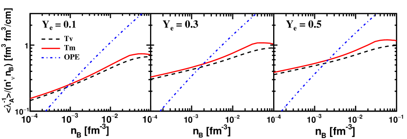
Figure 2: $\langle\lambda_{A}^{-1}\rangle/(n_{\nu}^{\prime}n_{B})$ as functions of density with the temperature given by Equation (14) and $Y_{e}=0.1,0.3$ and 0.5, respectively. The half-off-shell elements based on the vacuum $T$-matrix, in-medium $T$-matrix, and OPE potential have been used for comparison.

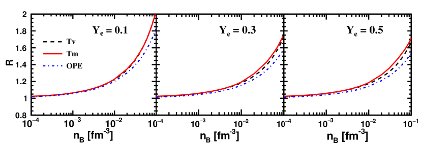
Figure 3: Ratios of $\langle\lambda_{A}^{-1}\rangle$ using the Boltzmann distribution without blocking to those using the Fermi distribution with blocking. The half-off-shell elements are used.

Figure 2 compares the results of $\langle\lambda_{A}^{-1}\rangle/(n_{\nu}^{\prime}n_{B})$ using the vacuum $T$-matrix, in-medium $T$-matrix, and the OPE potential. By dividing by the explicit factor $n_{B}$ in Equation (13), the value of $\langle\lambda_{A}^{-1}\rangle/(n_{\nu}^{\prime}n_{B})$ still increases with density as shown in Figure 2 due to the temperature dependence of Equation (14), which results in neutrinos with higher energies as the density grows. This will be further discussed when the normalized structure function is introduced.

Compared to the OPE potential, the $T$-matrix leads to an enhancement of $\langle\lambda_{A}^{-1}\rangle$ below $\sim$ 0.001–0.002 fm^-3, i.e., $\rho\sim(1.7\text{--}3.4)\times 10^{12}$ g cm^-3, and a suppression above. The enhancement at low densities for the $T$-matrix is due to the resonant property of the nuclear force (Bartl et al., 2014). At high densities, higher relative momenta become more relevant for which the $T$-matrix elements are suppressed and hence the inverse mean free path. Medium effects on the $T$-matrix lead to a slight increase in the bremsstrahlung rate by $\sim 10\%$. The effect is relatively small because for the conditions we consider in Equation (14) nucleons are not very degenerate, and meanwhile, the effects on the real and the imaginary parts of the $T$-matrix balance with each other. We choose to show the in-medium $T$-matrix results for the following studies but will not focus on the details.

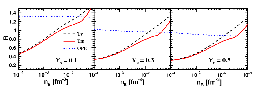
Figure 4: Ratios of $\langle\lambda_{A}^{-1}\rangle$ using the effective on-shell diagonal elements to those based on the half-off-shell/non-diagonal elements. The Fermi distribution with blocking is used.

Figure 3 shows the ratios of $\langle\lambda_{A}^{-1}\rangle$ using the Boltzmann distributions without blocking to those using the Fermi distributions with blocking, where the half-off-shell elements are used for both cases. The impact of blocking increases with density as the nucleon degeneracy increases. Using Equation (14), the degeneracy parameter for neutrons can be expressed as $\epsilon_{n}=E_{F}^{(n)}/T\simeq 0.1[\rho(1-Y_{e})/10^{11}~{}\text{g cm}^{-3}]^{1/3}\simeq 0.12[n_{B}(1-Y_{e})/10^{-4}\ \text{fm}^{-3}]^{1/3}$. We find that the Boltzmann approximations overestimate the opacity by $\sim$ 20% at $\epsilon_{n}\simeq 0.5$, i.e., at $n_{B}\simeq 10^{-2}\ \text{fm}^{-3}$, and by $\sim$ 50%–100% at $n_{B}\simeq 10^{-1}\ \text{fm}^{-3}$. As expected, the impact of the Pauli blocking is insensitive to the nuclear potentials used.

As given in Equations (A23) and (A26), the on-shell diagonal vacuum $T$-matrix is related to the experimentally measured phase shifts and mixing parameters; see Appendix A. This provides a method to estimate the on-shell diagonal elements of the $T$-matrix. Following Bartl et al. (2014), we use an effective on-shell element $\langle\bar{k}|\mathcal{T}|\bar{k}\rangle$ to approximate the half-off-shell and non-diagonal $T$-matrix element $\langle k_{f}|\mathcal{T}|k_{i}\rangle$ with $\bar{k}=\sqrt{(k_{i}^{2}+k_{f}^{2})/2}$. This approximation has been found to be reasonable for the OPE potential (Bartl et al., 2014). Compared to the studies based on the half-off-shell $T$-matrix, the effective on-shell matrix elements underestimate the rates significantly for densities $n_{B}\lesssim 10^{-2}$ fm^-3 by a factor up to $0.7$, and overestimate them above (see Figure 4). Therefore, the use of the half-off-shell $T$-matrix is required to reach an accurate bremsstrahlung rate.

3 Normalized structure function

The structure function, $S_{\sigma}(\omega)$, given in Equation (4) in the long-wavelength limit diverges as $\omega^{-2}$ for $\omega\to 0$, which is a common feature of any bremsstrahlung-type process (Raffelt et al., 1996). Though there is no divergence for the inverse mean free path $\langle\lambda^{-1}_{A}\rangle$ studied in Sec. 2.2, it may lead to an unphysical enhancement of $\lambda^{-1}_{A}(E_{\nu})$ in the limit of $E_{\nu}\to 0$. Hence, we want to obtain a well-behaved $S_{\sigma}(\omega)$ and study how the related rates are modified. It also provides a proper comparison with the existing studies with well-behaved structure functions (Hannestad & Raffelt, 1998; Raffelt, 2001; Bartl et al., 2014). This also allows us to extend the calculations to include RPA correlation effects based on a smooth $S_{\sigma}(\omega)$, as will be done in Sec. 4.

It has been suggested (see, e.g., Hannestad & Raffelt, 1998; Raffelt, 2001; Lykasov et al., 2008; Bacca et al., 2009, 2012; Roberts et al., 2012; Bartl et al., 2014; Roberts & Reddy, 2017) that the structure function can be regularized by replacing $\omega^{-2}$ with $(\omega^{2}+\Gamma^{2})^{-1}$, where the width parameter $\Gamma$ is introduced to characterize the spin fluctuation or relaxation rate. The axial structure function can also be viewed as a spin autocorrelation function, which is expected to decay exponentially as $\exp(-\Gamma t)$ at long times, leading to a Lorentzian form of $S_{\sigma}(\omega)$ (Hannestad & Raffelt, 1998; Raffelt, 2001). This is equivalent to considering that the nucleon propagator has a width due to nucleon-nucleon scattering in the nuclear medium, i.e., replacing $\omega^{-1}$ by $(\omega+i\Gamma)^{-1}$. Therefore, the proper renormalization of nucleons in the medium (also called ‘multiple-scattering’ effects in the literature, see, e.g., Hannestad & Raffelt, 1998) renders $S_{\sigma}(\omega)$ a well-behaved function. Studies based on Landau’s Fermi liquid theory that compute an energy-dependent relaxation rate also lead to a well-behaved $S_{\sigma}(\omega)$ (Lykasov et al., 2008; Bacca et al., 2009, 2012; Bartl et al., 2014; Bartl, 2016). Since the relaxation rate varies very slowly with $\omega$, we find that $S_{\sigma}(\omega)$ regularized by a constant $\Gamma$ agrees within a few per cent with the results of Bartl et al. (2014).

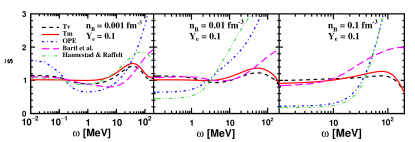
Figure 5: $\tilde{s}$ as functions of $\omega$ at $n_{B}=0.001$ fm^-3, 0.01 fm^-3 and 0.1 fm^-3, respectively, for $Y_{e}=0.1$. The half-off-shell matrix elements of the vacuum $T$-matrix, in-medium $T$-matrix, and OPE potential with the Pauli blocking are used. $\tilde{s}(\omega)$ from the fitting formulae in Hannestad & Raffelt (1998) based on the OPE potential, and obtained using the effective on-shell $T$-matrix following the formalism of Bartl et al. (2014), are also added for comparison.

The parameter $\Gamma$ can be determined by the normalization condition (Raffelt & Strobel, 1997; Hannestad & Raffelt, 1998):

$$\int_{-\infty}^{\infty}{d\omega\over 2\pi}S_{\sigma}(\omega) =\int_{0}^{\infty}{d\omega\over 2\pi}S_{\sigma}(\omega)(1+e^{-\omega/T})$$ (15)

$$={2\over n_{B}}\sum_{i=n,p}\int{d^{3}k\over(2\pi)^{3}}f_{i}(\varepsilon(k))[1-f_{i}(\varepsilon(k))],$$

with $\varepsilon(k)=k^{2}/(2m_{N})$ and $n_{B}$ the total nucleon number density. Note that the above equation is exact for a non-interacting system, and we assume that the main effect of nucleon-nucleon collisions is to increase the width of $S_{\sigma}(\omega)$ while keeping the normalization. Unless otherwise stated, $S_{\sigma}(\omega)$ refers to the properly normalized structure function, and we call the ones computed in Equations (4)-(7) unnormalized structure functions.

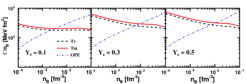
Figure 6: $\Gamma/n_{B}$ as a function of density based on different nuclear matrix elements for $Y_{e}=0.1$, 0.3, and 0.5, respectively.

The normalized $S_{\sigma}(\omega)$ can be expressed in Lorentzian form as (Hannestad & Raffelt, 1998; Raffelt, 2001; Lykasov et al., 2008; Bacca et al., 2009, 2012; Roberts et al., 2012; Bartl et al., 2014; Roberts & Reddy, 2017)

$$S_{\sigma}(\omega)=s(\omega)\frac{2\Gamma}{\omega^{2}+\Gamma^{2}},$$ (16)

where $s(\omega)$ is a dimensionless quantity that contains additional energy dependences originating from the nuclear correlations and blocking. For $\omega\ll\Gamma$, $s(\omega)\simeq 1$, and one has $S_{\sigma}(\omega)\simeq 2/\Gamma$; for $\omega\gg\Gamma$, $S_{\sigma}\simeq 2s(\omega)\Gamma/\omega^{2}$, which is fully determined by the perturbative calculation in Equations (4) and (5).

Taking as a reference the calculation based on the in-medium $T$-matrix, we introduce

$$\tilde{s}(\omega)\equiv S_{\sigma}(\omega)\frac{\omega^{2}+\Gamma_{T_{m}}^{2}}{2\Gamma_{T_{m}}}=\frac{S_{\sigma}(\omega)}{S^{T_{m}}_{\sigma}(\omega)}\tilde{s}^{T_{m}}(\omega),$$ (17)

with $\Gamma_{T_{m}}$, $S_{\sigma}^{T_{m}}$ and $\tilde{s}^{T_{m}}$ the width and structure functions using the in-medium $T$-matrix. We present the comparison of $\tilde{s}(\omega)$ in Figure 5 to show the relative differences in $S_{\sigma}(\omega)$ when using different approaches. Results based on the fitting formulae of the structure function from Hannestad & Raffelt (1998) consider only neutron-neutron interactions using the OPE potential. To demonstrate the effects of the off-shell elements and blocking, we also show the results based on the effective on-shell vacuum $T$-matrix following the formalism of Bartl et al. (2014), where the blocking effects are neglected and $S_{\sigma}(\omega)$ is normalized to $\sim$ 1; see Equation (15).

At low density condition where the blocking of the final nucleons can be ignored (see the left panel of Figure 5), we find an underestimation of $\tilde{s}(\omega)$, or $S_{\sigma}(\omega)$, at intermediate $\omega$ and an overestimation for high $\omega\gtrsim 20$ MeV, when the effective on-shell $T$-matrix elements are used. This is also consistent with the results shown in Figure 4, considering that $S_{\sigma}(\omega)$ for $\omega\sim 3T$ dominates the inverse mean free path, see Equation (13). As density increases, the Pauli blocking starts to play a role, and its impact becomes comparable to or even dominant over that of off-shell effects (see the middle and the right panels). For $\omega\gtrsim 10$ MeV, the off-shell effects and blocking together suppress $S_{\sigma}$ significantly. It is also interesting to notice that $s(\omega)$ based on the half-off-shell $T$-matrix including the blocking is close to 1 with a maximum deviation of $\sim$ 40%. For $s(\omega)\sim 1$, $S_{\sigma}(\omega)$ based on the $T$-matrix is simply determined by the width parameter; see Equation (16).

The behavior of $S_{\sigma}(\omega)$ for high values of $\omega$ is very important to the energy-averaged opacity against pair absorption (and bremsstrahlung energy loss rate) due to the factor of $\omega^{5}$ ($\omega^{6}$) in the integral [see Equations (13) and (11)]. As will be shown later, the combined effect of off-shell elements and blocking on $S_{\sigma}(\omega)$ at high $\omega$ can give rise to notable differences in $\langle\lambda_{A}^{-1}\rangle$.

Compared to the $T$-matrix, the OPE potential gives rise to a very different $S_{\sigma}(\omega)$, or $\tilde{s}(\omega)$. Since $S_{\sigma}(\omega\to 0)\simeq 2/\Gamma$, the value of $\tilde{s}(\omega)$ at small $\omega$ is determined by the width parameter $\Gamma$. The resonant property of the nuclear force exhibited in the $T$-matrix at low density (temperature) will lead to a larger $\Gamma$ and thus a smaller $S_{\sigma}(\omega)$ or $\tilde{s}(\omega)$ at small $\omega$. The $T$-matrix elements decrease rapidly with the relative momenta. For high values of $\omega$, the relative momenta between nucleons become large, leading to smaller values of $S_{\sigma}(\omega)$ than in the OPE results.

Studies by Hannestad & Raffelt (1998) consider only neutron-neutron interactions and hence our OPE results are close to theirs at low $Y_{e}$. Aside from the relatively small errors introduced in the fitting formulae of $S_{\sigma}(\omega)$ in Hannestad & Raffelt (1998), the remaining differences are due to the use of different $\pi NN$ coupling constants. We use $[g_{A}/(2F_{\pi})]^{4}$ in calculating the matrix element with $g_{A}=1.26$ and $F_{\pi}=92.4$ MeV, which is about $\sim 30$% smaller than $(f/m_{\pi})^{4}$ used in Hannestad & Raffelt (1998) with $f=1$ and $m_{\pi}$ the pion mass.

The corresponding values of $\Gamma/n_{B}$ required to normalize $S_{\sigma}(\omega)$ are shown in Figure 6 as a function of $n_{B}$. For $n_{B}$ around 0.01 fm^-3, $\Gamma$ can be as high as a few MeV. As already mentioned above, the resonant property at low energy/density and a rapidly decreasing $T$-matrix element with relative momenta are responsible for the enhancement/suppression of $\Gamma$ at low/high density compared to the OPE results. Furthermore, the behaviors of $\Gamma/n_{B}$ based on the $T$-matrix and the OPE potential can be understood in a more quantitative way as follows. At low energy, the $T$-matrix is dominated by the two resonant channels, ${}^{1}S_{0}$ and ${}^{3}S_{1}$, hence the corresponding hadronic part of the matrix element for $\omega\to 0$, $\bar{H}(k,k)$, varies with the relative momenta as $\bar{H}(k,k)\propto|T_{S=0,1}|^{2}\propto(a_{S=0,1}^{-2}+k^{2})^{-1}$, where $a_{S=0,1}$ are the scattering lengths. For comparison, the OPE potential leads to a different hadronic part, which takes a form like $\bar{H}(k,k)\propto k^{4}/(k^{2}+m_{\pi}^{2})^{2}$ (Hannestad & Raffelt, 1998). We consider the non-degenerate conditions where $k\sim\sqrt{Tm_{N}}$, and from the power counting of $T$ in Equation (7) for the unnormalized structure function we find $\Gamma/n_{B}\propto\lim_{\omega\to 0}[\omega^{2}S^{(0)}_{\sigma}(\omega)]/n_{B}\propto T^{1/2}(m_{N}T+\eta a^{-2})^{-1}$ for using the $T$-matrix, and $\Gamma/n_{B}\propto T(m_{N}T+\eta^{\prime}m_{\pi}^{2})^{-1/2}$ for using the OPE potential, with the coefficients $\eta,\eta^{\prime}\sim{\cal O}(1)$. Using the physical values for $a_{S=0,1}$, $m_{\pi}$ and $m_{N}$, one can explain the behavior of $\Gamma/n_{B}$ with density (or temperature) based on the $T$-matrix or the OPE potential shown in Figure 6.

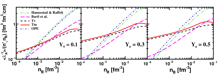
Figure 7: $\langle\lambda_{A}^{-1}\rangle/(n^{\prime}_{\nu}n_{B})$ based on normalised $S_{\sigma}$ as a function of density for $Y_{e}=0.1$, 0.3, and 0.5, respectively.

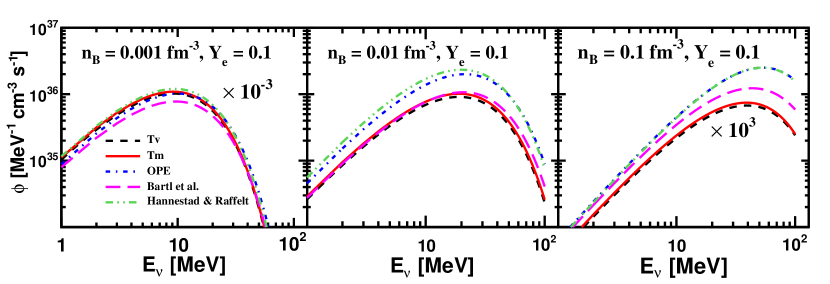
Figure 8: Emissivities of neutrinos from bremsstrahlung $\phi(E_{\nu})$, given in Equation (10), at $n_{B}=0.001,0.01$, and 0.1 fm^-3, respectively, for $Y_{e}=0.1$. Note that the results for $n_{B}=0.001$ and 0.1 fm^-3 shown in the plots need to be multiplied by an additional factors of $10^{-3}$ and $10^{3}$, respectively.

Figure 7 compares the results for $\langle\lambda_{A}^{-1}\rangle/(n_{B}n_{\nu}^{\prime})$ based on different normalized structure functions. The differences are simply due to different $S_{\sigma}(\omega)$ at high $\omega$, as shown in Figure 5. It should also be emphasized that $\langle\lambda_{A}^{-1}\rangle$ based on the normalized $S_{\sigma}$ are only slightly smaller (by up to $\sim$ 10%) than those based on the unnormalized ones; see Figure 2. Therefore, the studies of $\langle\lambda_{A}^{-1}\rangle$ based on the unnormalized structure functions in subsection 2.2 still hold.

A more relevant quantity to neutrino transport in supernova matter is the energy-dependent opacity against pair absorption, $\lambda_{A}^{-1}(E_{\nu})$, defined in Equation (8), and the neutrino emissivity from nucleon-nucleon bremsstrahlung, $\phi(E_{\nu})$, given in Equation (10) neglecting the final-state blocking of neutrinos. Since $\phi(E_{\nu})$ does not depend on the (anti)neutrino number density if the Pauli blocking is neglected, we choose to show $\phi(E_{\nu})$ in Figure 8 at $n_{B}=$ 0.001, 0.01, and 0.1 fm^-3, for $Y_{e}=0.1$. Note that $\lambda^{-1}_{A}(E_{\nu})$ can be obtained simply from $\phi(E_{\nu})$ with $\phi(E_{\nu})/\lambda_{A}^{-1}(E_{\nu})\propto E_{\nu}^{2}\exp(-E_{\nu}/T)$. At low density (temperature) or for low $E_{\nu}$, the $T$-matrix with half-off-shell matrix elements gives rise to the largest emissivities. As density (temperature) or $E_{\nu}$ increases, using the effective on-shell $T$-matrix or the OPE potential overestimates the emissivities. For the range of density and $E_{\nu}$ explored in Figure 8, the ratios of emissivities based on the effective on-shell $T$-matrix and the OPE potential to those based on the in-medium $T$-matrix with half-off-shell elements range from $\sim$ 0.5–1.8 and $\sim$ 0.7–5, respectively. Just as for the energy-averaged inverse mean free path $\langle\lambda_{A}^{-1}\rangle$, the medium effect on the $T$-matrix increases $\phi(E_{\nu})$ by $\lesssim$ (10–20)%.

We provide a numerical table of the normalized structure function $S_{\sigma}(\omega)$ based on the vacuum $T$-matrix for calculating the bremsstrahlung rate; see Appendix C. To implement the table in SN simulations, one has to do a 4D interpolation of the structure function over temperature, density, $Y_{e}$, and $\omega$. It should also be pointed out that, since we use exactly the same notation as that adopted in Hannestad & Raffelt (1998), the implementation of our new structure function should be similar.

4 RPA correlations

In addition to the multiple-scattering effects discussed above, there is another correlation effect that has been investigated within the framework of the RPA (Burrows & Sawyer, 1998; Reddy et al., 1999). Multiple-scattering effects account for the renormalization of the virtual nucleon propagator in the medium, while the RPA correlations screen the coupling between the leptonic weak current and the nucleons. Then, they can be treated as separate contributions in such a way that each nucleon propagator in the RPA ring diagrams is modified by multiple-scattering effects before performing the RPA summation. In this section, we discuss how the RPA correlation affects the structure function as well as the related rates.

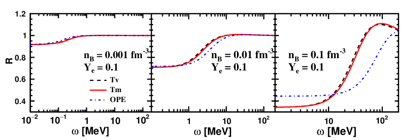
Figure 9: Effects of the RPA correlation on $S_{\sigma}(\omega)$ at $n_{B}=0.001$ fm^-3, 0.01 fm^-3, and 0.1 fm^-3, respectively, for $Y_{e}=0.1$. $R\equiv S_{\sigma}^{\text{RPA}}(\omega)/S_{\sigma}(\omega)$.

The RPA provides a formalism to account for the correlation effects by summing an infinite number of ring diagrams (Fetter & Walecka, 1971; Burrows & Sawyer, 1998; Reddy et al., 1999). Taking number density correlation for systems composed of one species as an example, the polarization function at the RPA level takes the form $\Pi_{\text{RPA}}(q,\omega)=\Pi_{u}(q,\omega)/[1-v(q)\Pi_{u}(q,\omega)]$, where $\Pi_{u}(q,\omega)$ is the polarization function without the RPA correlation and $v(q)$ is the spin-independent potential. As adopted in previous literature (Burrows & Sawyer, 1998; Reddy et al., 1999), $\Pi_{u}(q,\omega)$ can be taken to be the free polarization function $\Pi^{(0)}(q,\omega)$, which has an analytical expression and is the same for both density and spin-density correlations (Burrows & Sawyer, 1998; Reddy et al., 1998). In this work, we choose to consider the RPA corrections on top of our calculated structure function $S_{\sigma}(\omega)$, which already incorporates the multiple-scattering effects. We follow the formalism of Burrows & Sawyer (1998) based on a spin-dependent potential (see also Reddy et al., 1999; Horowitz & Schwenk, 2006; Horowitz et al., 2017). In principle, RPA calculations should be based on the same chiral potential as the one used for the $T$-matrix (Entem et al., 2017). However, the choice of Burrows & Sawyer (1998) leads to nucleon scattering rates within $\sim$ 10% of the model-independent studies based on virial expansion in the low-density region (Horowitz & Schwenk, 2006; Horowitz et al., 2017). On general grounds the effects of the RPA on the bremsstrahlung rates are expected to be smaller than for scattering; hence following the approach of Burrows & Sawyer (1998) provides a simple-to-implement method to quantify their relevance.

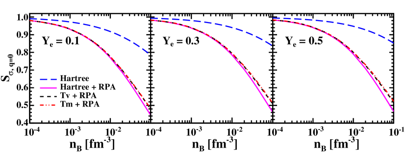
Figure 10: Static structure function in the long-wavelength limit, $S_{\sigma,q=0}$, as functions of density for $Y_{e}=0.1$, 0.3, and 0.5, respectively.

For a nuclear system consisting of protons and neutrons, the axial structure function (or the corresponding polarization functions) takes a $2\times 2$ matrix form as (Burrows & Sawyer, 1998)

$$\hat{S}_{\sigma}=\left[\begin{array}[]{cc}S_{\sigma}^{(pp)}&\frac{1}{2}S_{\sigma}^{(pn)}\\ \frac{1}{2}S_{\sigma}^{(np)}&S_{\sigma}^{(nn)}\end{array}\right],$$ (20)

where the different entries in the matrix contain contributions due to NN collisions described by the $T$-matrix. The total axial structure function $S_{\sigma}$ entering is given by $S_{\sigma}=S_{\sigma}^{(pp)}+S_{\sigma}^{(nn)}+\frac{1}{2}(S_{\sigma}^{(pn)}+S_{\sigma}^{(np)})=S_{\sigma}^{(pp)}+S_{\sigma}^{(nn)}+S_{\sigma}^{(np)}$, see Equation (5). Despite the fact that Burrows & Sawyer (1998) consider scattering and we are interested in bremsstrahlung, we find that their Equation (47) also applies to our case, and the structure function that includes both collision effects based on the $T$-matrix and the RPA correlation is given by

$$S_{\sigma}^{\text{RPA}}(\omega)=\frac{2}{n_{B}}\text{Im}[\Pi(\omega)][1-\exp(-\omega/T)]^{-1}{\cal C}_{A}^{-1},$$ (21)

where

$${\cal C}_{A}=\big{\{}1-v_{\text{GT}}\text{Re}[\Pi(\omega)]\big{\}}^{2}+v_{\text{GT}}^{2}\text{Im}[\Pi(\omega)]^{2},$$ (22)

with $v_{\text{GT}}=4.5\times 10^{-5}~{}\text{MeV}^{-2}$ and $\Pi(\omega)$ is given by

$$\text{Im}[\Pi(\omega)]= {n_{B}\over 2}S_{\sigma}(\omega)[1-\exp(-\omega/T)],$$ (23)

$$\text{Re}[\Pi(\omega)]= {1\over\pi}{\cal P}\int d\omega^{\prime}{\text{Im}[\Pi(\omega^{\prime})]\over\omega-\omega^{\prime}}.$$ (24)

Figure 9 shows how the normalized structure functions in Equation (15) based on different nuclear matrix elements are affected by RPA in different conditions with $R\equiv S^{\text{RPA}}_{\sigma}(\omega)/S_{\sigma}(\omega)$. The effect of the RPA correlation is to reduce $S_{\sigma}(\omega)$ at low $\omega$ due to a negative $\text{Re}[\Pi(\omega)]$, and to increase it slightly at high $\omega$ as $\text{Re}[\Pi(\omega)]$ turns positive. We also show in Figure 10 the effects of the RPA on the static structure function [or the normalization of $S_{\sigma}(\omega)$; see Equation (15)] in the long-wavelength limit, which is defined as

$$S_{\sigma,q=0}\equiv\lim_{q\to 0}\int_{-\infty}^{\infty}\frac{S_{\sigma}(q,\omega)}{2\pi}d\omega=\int_{-\infty}^{\infty}\frac{S_{\sigma}(\omega)}{2\pi}d\omega.$$ (25)

For comparison, we also present the mean-field or Hartree result (Reddy et al., 1998), which is simply given by Equation (15), the same as the static structure function associated with our normalized $S_{\sigma}(\omega)$ without including the effects of the RPA. The RPA correlations reduce $S_{\sigma,q=0}$, consistent with the studies based on virial expansion (Horowitz & Schwenk, 2006; Horowitz et al., 2017). Furthermore, we find a very similar reduction due to RPA correlations for the mean-field case and for cases that consider collisions based on the $T$-matrix. This justifies our assumption that the nucleon-nucleon collisional broadening does not affect the normalization of $S_{\sigma}(\omega)$, but just redistributes the strength in a broader energy region.

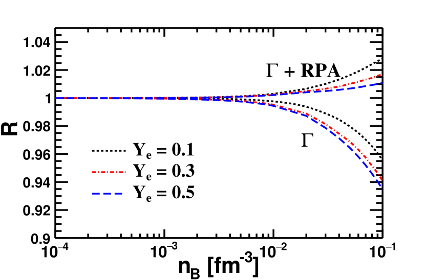
Figure 11: Ratios of $\langle\lambda_{A}^{-1}\rangle$ considering the effects of $\Gamma$ and the RPA correlation to those based on the unnormalized structure functions, as functions of density for $Y_{e}$=0.1, 0.3, and 0.5, respectively.

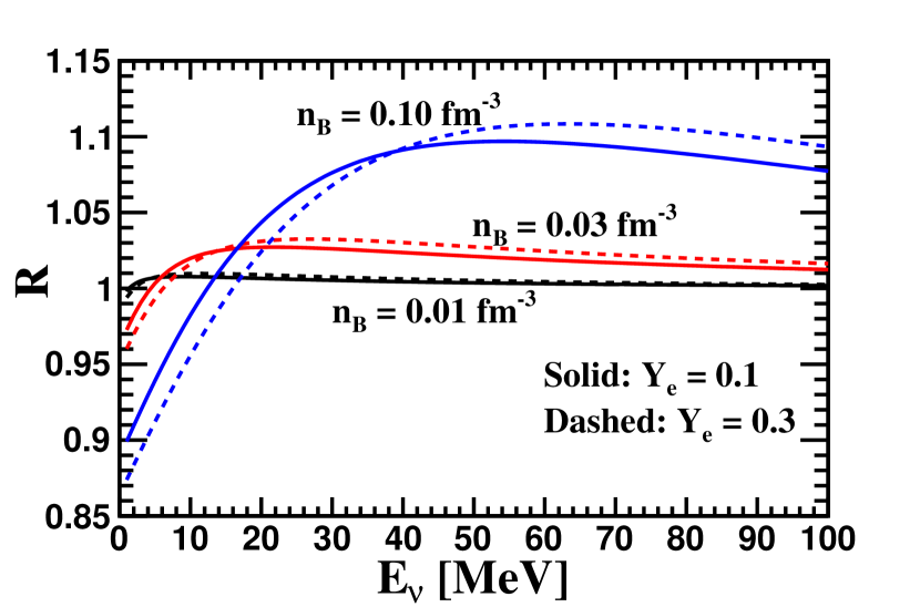
Figure 12: Ratios of $\lambda_{A}^{-1}(E_{\nu})$ with the RPA effect to those without at $n_{B}=0.01$, 0.03, and 0.1 fm^-3 and $Y_{e}$=0.1 and 0.3, respectively. The in-medium $T$-matrix elements are used for calculating $S_{\sigma}(\omega)$.

Figure 11 shows the effects of the RPA correlations and the width parameter $\Gamma$ on $\langle\lambda_{A}^{-1}\rangle$ as a function of density. As discussed above, the inclusion of $\Gamma$ only affects $S_{\sigma}(\omega)$ for $\omega\lesssim\Gamma$. However, $\langle\lambda_{A}^{-1}\rangle$ is determined by $S_{\sigma}(\omega)$ at high $\omega$ and hence the effect of $\Gamma$ is rather insignificant, reducing the rates by up to a few per cent at subsaturation densities. The average rate, $\langle\lambda_{A}^{-1}\rangle$, is enhanced slightly by the effects of the RPA, due to the increased $S_{\sigma}(\omega)$ in the high-$\omega$ region; see Figure 9. The combined effect of $\Gamma$ and RPA is $\sim$ 3% at most.

The effect of the RPA correlations on the energy-dependent inverse mean free path $\lambda_{A}^{-1}(E_{\nu})$ is illustrated in Figure 12 by showing the ratio of $\lambda^{-1}_{A}(E_{\nu})$ including RPA correlations to that without. The impact is similar to that on $S_{\sigma}(\omega)$ shown in Figure 9, i.e., a suppression in the low-energy region and an enhancement at high energy. We find that the effects become significant only for $n_{B}\gtrsim 0.01~{}\text{fm}^{-3}$ and can reach up to 10% near the saturation density, consistent with the results shown in Figure 11 for $\langle\lambda_{A}^{-1}\rangle$.

5 summary and conclusions

We have revisited the rate of neutrino bremsstrahlung in supernova matter in the long-wavelength limit and investigated the effects of different treatments in a systematic way. The vacuum/in-medium $T$-matrix for NN scattering with half-off-shell elements obtained by solving the Lippmann-Schwinger/Bethe-Goldstone equation based on $\chi$EFT potentials has been used to study the bremsstrahlung rates, to be compared with those based on the OPE potential and the associated diagonal/on-shell matrix elements. For a broad range of density, temperature, and $Y_{e}$ relevant to supernova conditions, we have considered the blocking of the final nucleons, which is to be compared with the studies using the Boltzmann distribution without blocking. We have also explored the effects of the width parameter, to account for multiple-scattering effects, and the RPA correlations on the structure function and the related rates. A numerical table of our new structure function based on the vacuum $T$-matrix is provided (see more details in Appendix C).

Taking Equation (14) to characterize the typical SN conditions, our studies show that ignoring the blocking of the final nucleons overestimates the rates by $\sim$ 20% at $n_{B}=0.01$ fm^-3 ($\rho\approx 1.7\times 10^{13}$ g cm^-3) and by $\sim$ 50%–100% at $n_{B}=0.1$ fm^-3 ($\rho\approx 1.7\times 10^{14}$ g cm^-3). Using the effective diagonal/on-shell $T$-matrix elements underestimates the rates by $\sim$ 50%–70% at $n_{B}=10^{-4}$ fm^-3 ($\rho\approx 1.7\times 10^{11}$ g cm^-3), and by $\sim$ 30%–50% at $n_{B}=10^{-3}$ fm^-3 ($\rho\approx 1.7\times 10^{12}$ g cm^-3), with the effects getting stronger with increasing $Y_{e}$. Close to the saturation density, the effective on-shell $T$-matrix gives rise to an enhancement by $\sim$ 20%–40%. We therefore argue that the half-off-shell $T$-matrix elements are required for an accurate study of the bremsstrahlung rate. We confirm the results of previous studies (Bartl et al., 2014; Bartl, 2016) that using the $T$-matrix element instead of the OPE potential leads to an enhancement by a factor of 2–5 at $n_{B}=10^{-4}$ fm^-3 ($\rho\approx 1.7\times 10^{11}$ g cm^-3) due to the resonant property of the NN force, and a suppression at densities above $\sim 2\times 10^{-3}$ fm^-3 ($\rho\approx 3.3\times 10^{11}$ g cm^-3). For the supernova-relevant conditions explored in this paper [see Equation (14)], we find that the results obtained using the standard vacuum $T$-matrix are very similar to those based on the in-medium $T$-matrix. Nevertheless, we expect that the differences will be larger for cold neutron stars where nucleons are highly degenerate.

Following Hannestad & Raffelt (1998), we introduce a width parameter or spin relaxation rate $\Gamma$ to normalise the axial structure function $S_{\sigma}(\omega)$ and to make a proper comparison with the previous studies in the literature (Raffelt, 2001; Lykasov et al., 2008; Bacca et al., 2009, 2012; Bartl et al., 2014). The effect of $\Gamma$ is to suppress $S_{\sigma}(\omega)$ at low $\omega$, and we find that the rates based on the normalized $S_{\sigma}(\omega)$ are only reduced by a few per cent for densities above $\sim$ 0.01 fm^-3 ($\rho\approx 1.7\times 10^{13}$ g cm^-3). Comparisons of neutrino pair absorption/emission rates based on our normalized $S_{\sigma}(\omega)$ to those from Hannestad & Raffelt (1998) and Bartl et al. (2014) are summarized in Figures 7 and 8. We find that the relative ratios of our results using the $T$-matrix to those from the previous literature could be either as small as $\sim$ 0.2, or as large as $\sim$ 5 for different regions of density and $E_{\nu}$ considered. The difference from Bartl et al. (2014) originates mainly from off-shell effects on the $T$-matrix as well as the blocking of the final nucleons.

Effects of the RPA correlation on top of the normalised $S_{\sigma}(\omega)$ that incorporates collisional broadening are further explored. We find that $S_{\sigma}(\omega)$ is reduced significantly at low $\omega$ and slightly enhanced at high $\omega$. Though the normalization of $S_{\sigma}(\omega)$ is reduced, which is consistent with the prediction from virial expansion, the energy-averaged inverse mean free path $\langle\lambda_{A}^{-1}\rangle$ is slightly enhanced by $\lesssim$ (2–3)% below the saturation density. Similarly to $S_{\sigma}(\omega)$, $\lambda_{A}^{-1}(E_{\nu})$ is suppressed at low $E_{\nu}$ and enhanced at high $E_{\nu}$ by the RPA correlations, but only by a negligible factor that is within a few per cent for the relevant conditions.

The impact of neutrino bremsstrahlung rates beyond OPE has been explored in 1D supernova simulations (Bartl et al., 2016; Fischer, 2016) (see also Raffelt, 2001; Keil et al., 2003, for studies based on bremsstrahlung rates using the OPE potential). Our calculations based on the half-off-shell $T$-matrix, similarly to those of Bartl et al. (2014), predict a low-density resonant enhancement of the bremsstrahlung rate $\langle\lambda_{A}^{-1}\rangle$ and a suppression at high densities when compared with the OPE results (see Figure 7). Bartl et al. (2014) predict a transition density that is typically smaller than the value reached at the neutrinosphere, which moves from $\rho\sim 10^{12}$ g cm^-3 to $10^{14}$ g cm^-3 as the PNS deleptonizes. Hence, the net effect in the supernova simulations of Bartl et al. (2016) is a reduction of the bremsstrahlung rate by a factor of $\sim$ 2–5 when compared with the OPE rates. Such a reduction translates into a minor change in the neutrino luminosities ($\lesssim 5\%$) and a small increase of the averaged neutrino energies, $\langle E_{\nu}\rangle$, within 1 MeV. In our calculations, the transition density is shifted to higher densities similar to those in the neutrinosphere. This may indicate an even smaller impact on the neutrino emission of the rates presented here. However, given the nonlinear nature of neutrino processes in supernova matter, a fully self-consistent simulation is required to quantify their impact.

We expect that the improved treatment of the NN interaction presented in this work will significantly affect the inelastic scattering process, $\nu+N+N\to\nu+N+N$, which should exhibit more relevance in SN dynamics (Sawyer, 1995; Raffelt & Strobel, 1997; Hannestad & Raffelt, 1998; Raffelt, 2001; Melson et al., 2015; Burrows et al., 2018; Kotake et al., 2018). In principle, the same structure function, $S_{\sigma}(q,\omega)$, governs both neutrino scattering and bremsstrahlung as well as pair absorption in the nuclear medium, though different regions in $(q,\omega)$ are relevant to each process, i.e., $q^{2}\leq\omega^{2}$ for pair absorption and bremsstrahlung, and $q^{2}\geq\omega^{2}$ for inelastic scattering. To obtain $S_{\sigma}$ in this work, we have taken the long-wavelength limit and therefore ignored the recoil of nucleons. This is a good approximation for studying pair absorption and bremsstrahlung, since the recoil energy, $E_{r}$, is always negligible compared to the energy transfer or the width parameter, i.e., $E_{r}\sim qP_{N}/m_{N}\sim(T/m_{N})^{1/2}q\lesssim(T/m_{N})^{1/2}\omega\ll\text{max}(\omega,\Gamma)$ with $P_{N}$ the typical nucleon momentum. We have checked by using the OPE potential that nucleon recoil affects the associated rates by only a few per cent for typical SN conditions. However, this is not the case for inelastic scattering, since $q$ is typically of the order of $E_{\nu}$ or $E_{\nu}^{\prime}$, and could be much larger than $\omega=E_{\nu}-E_{\nu}^{\prime}$, which vanishes in the elastic limit. Therefore, the nucleon recoil is no longer negligible (Raffelt, 2001). We argue that the studies of $S_{\sigma}(\omega)$ in this work should still be reliable for studying neutrino scattering in the limit of $E_{r}\sim\text{max}(E_{\nu},E_{\nu}^{\prime})\times(T/m_{N})^{1/2}\ll\Gamma$. In the opposite limit where $\Gamma$ is negligible compared to $E_{r}$ and $\omega$, $S(q,\omega)$ has an analytical expression including the recoil effect (Burrows & Sawyer, 1998; Reddy et al., 1998; Raffelt, 2001). We plan to provide a full treatment of $S_{\sigma}(q,\omega)$ incorporating both the collisional broadening and the nucleon recoils in the future work.

Appendix A $T$-matrix elements in vacuum/nuclear medium

The relevant formulae for obtaining the NN scattering $T$-matrix elements in vacuum/nuclear medium are shown below.

A.1 vacuum $T$-matrix

The vacuum $T$-matrix can be obtained from the Lippmann-Schwinger (LS) equation as

$$\mathcal{T}(\bm{k}^{\prime},\bm{k};E)=V(\bm{k}^{\prime},\bm{k})+\int{d^{3}k^{\prime\prime}\over(2\pi)^{3}}V(\bm{k}^{\prime},\bm{k}^{\prime\prime}){1\over E-{k^{\prime\prime 2}\over m_{N}}+i\varepsilon}\mathcal{T}(\bm{k}^{\prime\prime},\bm{k};E),$$ (A1)

where $\bm{k}$ ($\bm{k}^{\prime})$ is the relative momentum between the two incoming (outgoing) nucleons, and we adopt the notation $k\equiv|\bm{k}|$. We usually call the $T$-matrix on-shell when $E=k^{\prime 2}/m_{N}=k^{2}/m_{N}$, half-off-shell when one of them holds, or off-shell when neither holds.

In partial wave components, the LS equation can be cast as

$$\mathcal{T}^{JST}_{ll^{\prime}}(k^{\prime},k;E)=V^{JST}_{ll^{\prime}}(k^{\prime},k)+\sum_{l^{\prime\prime}}\int{k^{\prime\prime 2}dk^{\prime\prime}\over(2\pi)^{3}}V^{JST}_{ll^{\prime\prime}}(k^{\prime},k^{\prime\prime}){1\over E-{k^{\prime\prime 2}\over m_{N}}+i\varepsilon}\mathcal{T}^{JST}_{ll^{\prime\prime}}(k^{\prime\prime},k;E),$$ (A2)

where indices $J,S$ and $T$ are the three conserved quantum numbers: the total angular momentum, the total spin, and the total isospin of the nucleon pair; and $l,l^{\prime}$ are the relative orbital angular momenta for the incoming and outgoing nucleon pairs. Note that the coupling of partial waves with different $l$ arises from the tensor part of the nuclear force, which does not conserve the angular momentum $l$. Due to the conservation of $J$ ($\vec{J}=\vec{l}+\vec{S}$) and parity $\Pi=(-1)^{l}$, the only allowed values of $\Delta l\equiv l-l^{\prime}$ are 0, $\pm 2$. Another selection rule from the Pauli exclusion principle is that $l+S+T$ should be odd.

The LS equation [Equation (A2)] can be numerically solved by matrix inversion after discretizing the integral into a sum (Haftel & Tabakin, 1970; Machleidt, 1993, 2001). Note that the factor $i\varepsilon$ in the denominator coupling the real and imaginary parts of the $T$-matrix makes the calculation more involved. A more efficient way is to deal with the real $R$-matrix (or $K$-matrix), which is defined as (Landau, 1990)

$$\mathcal{R}=\mathcal{T}+i\pi\mathcal{T}\delta(E-H_{0})\mathcal{R},$$ (A3)

and the $R$-matrix obeys a ‘real’ version of the LS equation as

$$\mathcal{R}^{JST}_{ll^{\prime}}(k^{\prime},k;E)=V^{JST}_{ll^{\prime}}(k^{\prime},k)+\sum_{l^{\prime\prime}}\int{k^{\prime\prime 2}dk^{\prime\prime}\over(2\pi)^{3}}V^{JST}_{ll^{\prime\prime}}(k^{\prime},k^{\prime\prime}){\cal P}\Big{[}{1\over E-{k^{\prime\prime 2}\over m_{N}}}\Big{]}\mathcal{R}^{JST}_{ll^{\prime\prime}}(k^{\prime\prime},k;E).$$ (A4)

Once $\mathcal{R}^{JST}_{ll^{\prime}}$ is known, we can obtain the components of the $T$-matrix from Equation (A3). For a half-off-shell $T$-matrix, we need to solve

$$\mathcal{T}^{JST}_{ll^{\prime}}(k,k_{0};E_{k_{0}})\Big{[}\delta_{l^{\prime}l^{\prime\prime}}+i\pi\frac{m_{N}k_{0}}{2(2\pi)^{3}}\mathcal{R}^{JST}_{l^{\prime}l^{\prime\prime}}(k_{0},k_{0};E_{k_{0}})\Big{]}=\mathcal{R}^{JST}_{ll^{\prime\prime}}(k,k_{0};E_{k_{0}}),$$ (A5)

with $E_{k_{0}}=k_{0}^{2}/m_{N}$. This can be further simplified for uncoupled channels (with $l=l^{\prime}$) to

$$\mathcal{T}^{JST}_{ll}(k,k_{0};E_{k_{0}})={\mathcal{R}^{JST}_{ll}(k,k_{0};E_{k_{0}})\over 1+i\pi{m_{N}k_{0}\over 2(2\pi)^{3}}\mathcal{R}_{ll}(k_{0},k_{0};E_{k_{0}})},$$ (A6)

with

$$\text{Re}[\mathcal{T}^{JST}_{ll}(k,k_{0};E_{k_{0}})]={\mathcal{R}^{JST}_{ll}(k,k_{0};E_{k_{0}})\over 1+[\pi{m_{N}k_{0}\over 2(2\pi)^{3}}\mathcal{R}^{JST}_{ll}(k_{0},k_{0};E_{k_{0}})]^{2}},$$ (A7)

$$\text{Im}[\mathcal{T}^{JST}_{ll}(k,k_{0};E_{k_{0}})]={-\pi{m_{N}k_{0}\over 2(2\pi)^{3}}\mathcal{R}^{JST}_{ll}(k,k_{0};E_{k_{0}})\mathcal{R}^{JST}_{ll}(k_{0},k_{0};E_{k_{0}})\over 1+[\pi{m_{N}k_{0}\over 2(2\pi)^{3}}\mathcal{R}^{JST}_{ll}(k_{0},k_{0};E_{k_{0}})]^{2}}.$$ (A8)

The phase shifts for uncoupled channels are simply given by (Machleidt, 2001)

$$\tan\delta^{JST}_{l}(E_{k_{0}})=-\frac{\pi k_{0}m_{N}}{2(2\pi)^{3}}\mathcal{R}^{JST}_{ll}(k_{0},k_{0};E_{k_{0}}),$$ (A9)

and for coupled channels we have

$$U^{-1}\left[\begin{array}[]{cc}\tan\delta^{J}_{J-1}(E_{k_{0}})&0\\ 0&\tan\delta^{J}_{J+1}(E_{k_{0}})\end{array}\right]U=-\frac{\pi k_{0}m_{N}}{2(2\pi)^{3}}\left[\begin{array}[]{cc}\mathcal{R}^{J}_{J-1,J-1}(k_{0},k_{0};E_{k_{0}})&\mathcal{R}^{J}_{J-1,J+1}(k_{0},k_{0};E_{k_{0}})\\ \mathcal{R}^{J}_{J+1,J-1}(k_{0},k_{0};E_{k_{0}})&\mathcal{R}^{J}_{J+1,J+1}(k_{0},k_{0};E_{k_{0}})\end{array}\right],$$ (A14)

with $U$ the standard $2\times 2$ mixing matrix given by

$$U=\left[\begin{array}[]{cc}\cos\varepsilon^{J}&\sin\varepsilon^{J}\\ -\sin\varepsilon^{J}&\cos\varepsilon^{J}\end{array}\right].$$ (A17)

Note that we are allowed to drop the indices $S,T$ for coupled channels without introducing any confusion since they are fixed for a given $J$ (i.e., use $\delta^{J}_{J\pm 1}$, $\varepsilon^{J}$ and $\mathcal{R}^{J}_{J\pm 1,J\pm 1}$). From Equation (A14), we can obtain

$$\tan 2\varepsilon^{J}(E_{k_{0}})=\frac{2\mathcal{R}^{J}_{J+1,J-1}}{\mathcal{R}^{J}_{J-1,J-1}-\mathcal{R}^{J}_{J+1,J+1}},$$ (A18)

$$\tan\delta^{J}_{J\mp 1}(E_{k_{0}})=-\frac{\pi k_{0}m_{N}}{4(2\pi)^{3}}\Big{[}\mathcal{R}^{J}_{J-1,J-1}+\mathcal{R}^{J}_{J+1,J+1}\pm\frac{\mathcal{R}^{J}_{J-1,J-1}-\mathcal{R}^{J}_{J+1,J+1}}{\cos 2\varepsilon^{J}(E_{k_{0}})}\Big{]}.$$ (A19)

Once the phase parameters $\varepsilon^{J}$ and $\delta^{J}_{J\pm 1}$ are fixed from the $R$-matrix elements, the $T$-matrix elements for the coupled channels can be obtained from Equation (A5) as

$$\mathcal{T}^{J}_{ll^{\prime}}(k,k_{0};E_{k_{0}})=\mathcal{R}^{J}_{ll^{\prime\prime}}(k,k_{0};E_{k_{0}})U^{-1}_{l^{\prime\prime}\tilde{l}}\left[\begin{array}[]{cc}1-i\tan\delta^{J}_{J-1}&0\\ 0&1-i\tan\delta^{J}_{J+1}\end{array}\right]^{-1}_{\tilde{l}\tilde{\tilde{l}}}U_{\tilde{\tilde{l}}l^{\prime}}.$$ (A22)

The above phase shifts and mixing parameters for coupled channels are defined in the so-called ‘BB’ convention (Blatt & Biedenharn, 1952). An alternative convention for the phase parameters is proposed in Stapp et al. (1957), which is known as the ‘bar’ convention, and is usually adopted for analyzing NN scattering data. The two conventions are the same for uncoupled channels but different for the coupled channels. In the ‘bar’ convention, the on-shell $T$-matrix is given by

$$\mathcal{T}^{JST}_{ll^{\prime}}(k_{0},k_{0};E_{k_{0}})=-\frac{8\pi^{2}}{im_{N}k_{0}}[\exp(2i\bar{\delta}^{JST}_{l})-1]$$ (A23)

for uncoupled channels, and

$$\mathcal{T}^{JST}_{ll^{\prime}}(k_{0},k_{0};E_{k_{0}})=-\frac{8\pi^{2}}{im_{N}k_{0}}\times\left\{\begin{array}[]{c}[\exp(2i\bar{\delta}^{J}_{l})\cos 2\bar{\varepsilon}^{J}-1]~{}~{}\text{for $l=l^{\prime}$,}\\ i\exp[i(\bar{\delta}^{J}_{l}+\bar{\delta}^{J}_{l^{\prime}})]\sin 2\bar{\varepsilon}^{J}~{}~{}\text{for $l\neq l^{\prime}$,}\end{array}\right.$$ (A26)

for coupled channels. Note that only the on-shell $T$-matrix elements can be obtained from measured phase shifts; in order to obtain the off-shell elements, the LS equation should be solved based on a given nuclear potential.

A.2 in-medium $T$-matrix

The discussion for the vacuum $T$-matrix can be applied to the in-medium $T$-matrix using the Bethe-Goldstone (BG) equation,

$$\mathcal{T}^{JST}_{ll^{\prime}}(k^{\prime},k;K,\Omega)=V^{JST}_{ll^{\prime}}(k^{\prime},k)+\sum_{l^{\prime\prime}}\int{k^{\prime\prime 2}dk^{\prime\prime}\over(2\pi)^{3}}V^{JST}_{ll^{\prime\prime}}(k^{\prime},k^{\prime\prime})\bar{g}_{II}(K,\Omega,k^{\prime\prime})\mathcal{T}^{JST}_{l^{\prime\prime}l}(k^{\prime\prime},k;K,\Omega),$$ (A27)

where $\bar{g}_{II}(K,\Omega,k^{\prime\prime})$ is an angle-averaged two-particle propagator, which in the quasiparticle approximation is given by

$$\bar{g}_{II}(K,\Omega,k)=\biggl{\langle}\frac{1-f(\varepsilon(k_{1}))-f(\varepsilon(k_{2}))}{\Omega-\varepsilon(k_{1})-\varepsilon(k_{2})+i\eta}\biggr{\rangle}_{\theta},$$ (A28)

with the two nucleon momenta $\bm{k}_{1,2}={1\over 2}\bm{K}\pm\bm{k}$ and $\theta$ the angle between the total momentum $\bm{K}$ and the relative momentum $\bm{k}$. $\Omega$ is the total energy of the nucleon pair and $\varepsilon(k_{1,2})$ is the non-relativistic single-particle energy of the nucleon that in the quasiparticle approximation can be given by $\varepsilon(k_{i})=k_{i}^{2}/(2m^{*}_{n,p})+U_{n,p}$, where $m^{*}_{n,p}$ and $U_{n,p}$ are the effective masses and interacting potentials of neutron and proton in the nuclear medium. The Fermi function takes the standard form as $f(\varepsilon)=1/[1+\exp\big{(}\frac{\varepsilon-\mu}{k_{B}T}\big{)}]$ with $\mu$ the non-relativistic chemical potential of the nucleon. In the low-density limit, we have $\varepsilon(k_{1,2})\to\varepsilon_{0}(k_{1,2})=k_{1,2}^{2}/(2m_{N})$ and $1-\varepsilon((k_{1}))-f(\varepsilon(k_{2}))\to 1$, and therefore $\bar{g}_{II}(K,\Omega,p)\to(E-k^{2}/m_{N}+i\eta)^{-1}$ with $E=\Omega-K^{2}/(4m_{N})$ and $m_{N}=(m_{n}+m_{p})/2$ the averaged nucleon bare mass.

Exactly the same procedures are taken to numerically solve the in-medium $T$-matrix. Once the partial wave components of the $R$-matrix are obtained from matrix inversion, one can use Equations (A6) and (A22) to obtain the $T$-matrix elements, but with the replacement of $k_{0}m_{N}$ by $2k_{0}^{2}\langle 1-f(\varepsilon(k_{1}))-f(\varepsilon(k_{2}))\rangle_{\theta}[d\langle\varepsilon(k_{1})+\varepsilon(k_{2})\rangle_{\theta}/dk|_{k=k_{0}}]^{-1}$ at $\Omega=\langle\varepsilon(k_{1})+\varepsilon(k_{2})\rangle_{\theta}$ for any given value of $K$ [see Equations (A6) and (A19)]. In the low-density limit we have $\langle\varepsilon(k_{1})+\varepsilon(k_{2})\rangle_{\theta}={K^{2}\over 4m_{N}}+{k^{2}\over m_{N}}$, $f(\epsilon(k_{1,2}))\ll 1$, and therefore $d\langle\varepsilon(k_{1})+\varepsilon(k_{2})\rangle_{\theta}/dk|_{k=k_{0}}=2k_{0}/m_{N}$, which guarantees that the in-medium $T$-matrix goes to the vacuum one.

Throughout this work, we always take the bare nucleon mass for all our studies. For bremsstrahlung, the nucleon interaction potentials can be absorbed into the chemical potentials and we can simply take $U_{n,p}$=0 without affecting the final results. As can be easily seen, the medium effects on the $T$-matrix considered in this work are mainly from the blocking factor in Equation (A28).

Appendix B matrix elements for NN bremsstrahlung in partial wave components

Bartl et al. (2014) and Bartl (2016) have developed a formalism for the calculation of matrix elements of NN bremsstrahlung in partial wave components within the long-wavelength approximation in the $pn$-formalism. In the following, we present an alternative derivation using the isospin formalism.

Let us consider the process (see Figure 1)

$$N_{a}+N_{b}\rightarrow N_{c}+N_{d}+\nu+\bar{\nu},$$ (B1)

where $N$ stands for either a neutron, $n$, or a proton, $p$. Energy and momentum conservations imply

$$\bm{k}_{a}+\bm{k}_{b} = \bm{k}_{c}+\bm{k}_{d}+\bm{q},$$ (B2a)

$$E_{a}+E_{b} = E_{c}+E_{d}+\omega.$$ (B2b)

In the following, we will consider the long-wavelength limit in which neutrinos carry away zero momentum, i.e., $\bm{q}=\bm{0}$. We define the relative momenta of the nucleons as

$$\bm{k}_{i}=\frac{\bm{k}_{a}-\bm{k}_{b}}{2},\quad\bm{k}_{f}=\frac{\bm{k}_{c}-\bm{k}_{d}}{2}.$$ (B3)

As the center-of-mass momentum of the nucleons is conserved, we consider states that are characterized by the relative momenta of the nucleons and their spin projections, $|ab\rangle=|\bm{k}\,s_{a}s_{b}\rangle$ normalized such as

$$\langle\bm{k}_{f}\,s_{c}s_{d}|\bm{k}_{i}\,s_{a}s_{b}\rangle=(2\pi)^{3}\delta(\bm{k}_{i}-\bm{k}_{f})\delta_{s_{a}s_{c}}\delta_{s_{b}s_{d}}.$$ (B4)

We can build fully antisymmetric states using the permutation operator $P_{12}$ as

$$|ab\rangle_{\text{nas}}=|\bm{k}\,s_{a}s_{b}\rangle_{\text{nas}}=\frac{1}{\sqrt{2}}(1-P_{12})|\bm{k}\,s_{a}s_{b}\rangle=\frac{1}{\sqrt{2}}\Bigl{[}|\bm{k}\,s_{a}s_{b}\rangle-|-\bm{k}\,s_{b}s_{a}\rangle\Bigr{]}.$$ (B5)

States of good spin and isospin are obtained as

$$|\bm{k}\,SS_{z}\,TT_{z}\rangle=\sum_{s_{a}s_{b}t_{c}t_{d}}\langle 1/2\,s_{a}\,1/2\,s_{b}|S\,S_{z}\rangle\langle 1/2\,t_{a}\,1/2\,t_{b}|T\,T_{z}\rangle|\bm{k}\,s_{a}s_{b}\,t_{a}t_{b}\rangle,$$ (B6)

where we use the convention of neutrons having isospin projection 1/2. Expanding the plane wave states into partial waves, we obtain

$$|\bm{k}\,SS_{z}\,TT_{z}\rangle=\sum_{lm}Y^{*}_{lm}(\hat{\bm{k}})|k\,lm\,SS_{z}\,TT_{z}\rangle,$$ (B7)

with $\hat{\bm{k}}$ the unit vector in the direction of $\bm{k}$ and $k=|\bm{k}|$. The partial wave states are normalized as

$$\langle k_{f}\,l_{f}m_{f}\,S_{f}S_{z,f}\,T_{f}T_{z,f}|k_{i}\,l_{i}m_{i}\,S_{i}S_{z,i}\,T_{i}T_{z,i}\rangle=(2\pi)^{3}\frac{\delta(k_{i}-k_{f})}{k_{i}^{2}}\delta_{l_{f}l_{i}}\delta_{m_{f}m_{i}}\delta_{S_{f}S_{i}}\delta_{S_{z,f}S_{z,i}}\delta_{T_{f}T_{i}}\delta_{T_{z,f}T_{z,i}}.$$ (B8)

Coupling the orbital angular momentum and spin, we finally have states

$$|k\,lSJM\,TT_{z}\rangle=\sum_{mS_{z}}\langle l\,m\,S\,S_{z}|J\,M\rangle|k\,lm\,SS_{z}\,TT_{z}\rangle.$$ (B9)

We can build normalized antisymmetric states using the permutation operator, e.g.,

$$|\bm{k}\,SS_{z}\,TT_{z}\rangle_{\text{nas}}=\frac{1-P_{12}}{\sqrt{2}}|\bm{k}\,SS_{z}\,TT_{z}\rangle=\sum_{lm}\frac{1-(-1)^{l+S+T}}{\sqrt{2}}Y^{*}_{lm}(\hat{\bm{k}})|k\,lm\,SS_{z}\,TT_{z}\rangle=\sum_{lm}Y^{*}_{lm}(\hat{\bm{k}})|k\,lm\,SS_{z}\,TT_{z}\rangle_{\text{nas}}.$$ (B10)

The calculation of the matrix element for NN bremsstrahlung requires the evaluation of the spatial trace of the hadronic tensor (Raffelt & Seckel, 1995; Hannestad & Raffelt, 1998). This includes contributions from the eight diagrams given in Figure 1 (see also Friman & Maxwell, 1979), which give for the $nn$ or $pp$ channel

$$\bar{H}^{(nn)}=\bar{H}^{(pp)} = \frac{1}{3}\sum_{s_{a}s_{b}s_{c}s_{d}u}|{}_{\text{nas}}\langle\bm{k}_{f}\,s_{c}s_{d}|\bm{\mathcal{O}}_{u}|\bm{k}_{i}\,s_{a}s_{b}\rangle_{\text{nas}}|^{2}$$ (B11)

$$= \frac{1}{3\cdot 4}\sum_{s_{a}s_{b}s_{c}s_{d}u}(-1)^{1+u}\langle\bm{k}_{f}\,s_{c}s_{d}|\bm{\mathcal{O}}_{u}(1-P_{12})|\bm{k}_{i}\,s_{a}s_{b}\rangle\langle\bm{k}_{i}\,s_{a}s_{b}|\tilde{\bm{\mathcal{O}}}_{-u}(1-P_{12})|\bm{k}_{f}\,s_{c}s_{d}\rangle,$$

where the sum on $u$ runs over the spherical components, $0$ and $\pm 1$, of the vector operator $\bm{\mathcal{O}}$ that satisfies $(\bm{\mathrm{O}}_{u})^{\dagger}=(-1)^{1+u}\tilde{\bm{\mathrm{O}}}_{-u}$. We have used non-antisymmetric states to explicitly show the direct and exchange contributions. Expressions for the operator $\bm{\mathcal{O}}$ within the long-wavelength limit used in the present work will be provided later. For the moment, we keep the formalism fully general. The obtained expressions are then also applicable for more sophisticated treatments of the nuclear weak current and/or the intermediate nucleon propagator. Using states of total spin $S$ and isospin $T$ we have

$$\bar{H}^{(nn)} = \frac{-1}{3\cdot 4}\sum_{\begin{subarray}{c}S_{f}S_{z,f}\\ S_{i}S_{z,i}\\ u\end{subarray}}(-1)^{u}\langle\bm{k}_{f}\,S_{f}S_{z,f}\,1\,1|\bm{\mathcal{O}}_{u}(1-P_{12})|\bm{k}_{i}\,S_{i}S_{z,i}\,1\,1\rangle\langle\bm{k}_{i}\,S_{i}S_{z,i}\,1\,1|\tilde{\bm{\mathcal{O}}}_{-u}(1-P_{12})|\bm{k}_{f}\,S_{f}S_{z,f}\,1\,1\rangle,$$ (B12a)

$$\bar{H}^{(pp)} = \frac{-1}{3\cdot 4}\sum_{\begin{subarray}{c}S_{f}S_{z,f}\\ S_{i}S_{z,i}\\ u\end{subarray}}(-1)^{u}\langle\bm{k}_{f}\,S_{f}S_{z,f}\,1\,{-1}|\bm{\mathcal{O}}_{u}(1-P_{12})|\bm{k}_{i}\,S_{i}S_{z,i}\,1\,{-1}\rangle\langle\bm{k}_{i}\,S_{i}S_{z,i}\,1\,{-1}|\tilde{\bm{\mathcal{O}}}_{-u}(1-P_{12})|\bm{k}_{f}\,S_{f}S_{z,f}\,1\,{-1}\rangle.$$

For the $np$ case the direct and exchange terms correspond to physically different processes whose contribution needs to be summed. We obtain

$$\bar{H}^{(np)}=\frac{1}{3}\sum_{\begin{subarray}{c}S_{f}S_{z,f}\\ S_{i}S_{z,i}\\ u\end{subarray}}|\langle\bm{k}_{f}S_{f}\,S_{z,f}|\bm{O}_{u}(1-P_{12})|\bm{k}_{i}S_{i}\,S_{z,i}\rangle|^{2},$$ (B13)

which gives for isospin states

$$\bar{H}^{(np)}=\frac{-1}{3\cdot 4}\sum_{\begin{subarray}{c}S_{f}S_{z,f}T_{f}\\ S_{i}S_{z,i}T_{i}\\ T^{\prime}_{f}T^{\prime}_{i}u\end{subarray}}(-1)^{u}\langle\bm{k}_{f}\,S_{f}S_{z,f}\,T_{f}0|\bm{\mathcal{O}}_{u}(1-P_{12})|\bm{k}_{i}\,S_{i}S_{z,i}\,T_{i}0\rangle\langle\bm{k}_{i}\,S_{i}S_{z,i}\,T^{\prime}_{i}0|\tilde{\bm{\mathcal{O}}}_{-u}(1-P_{12})|\bm{k}_{f}\,S_{f}S_{z,f}\,T^{\prime}_{f}0\rangle.$$ (B14)

In the following we provide formulas to evaluate the necessary matrix elements using standard angular momentum algebra. We need to evaluate the following matrix elements:

$$\bar{H}(T_{z})=\frac{-1}{3\cdot 4}\sum_{\begin{subarray}{c}S_{f}S_{z,f}T_{f}\\ S_{i}S_{z,i}T_{i}\\ T^{\prime}_{f}T^{\prime}_{i}u\end{subarray}}(-1)^{u}\langle\bm{k}_{f}\,S_{f}S_{z,f}\,T_{f}T_{z}|\bm{\mathcal{O}}_{u}(1-P_{12})|\bm{k}_{i}\,S_{i}S_{z,i}\,T_{i}T_{z}\rangle\langle\bm{k}_{i}\,S_{i}S_{z,i}\,T^{\prime}_{i}T_{z}|\tilde{\bm{\mathcal{O}}}_{-u}(1-P_{12})|\bm{k}_{f}\,S_{f}S_{z,f}\,T^{\prime}_{f}T_{z}\rangle,$$ (B15)

with $\bar{H}^{(nn)}=\bar{H}(T_{z}=1)=\bar{H}^{(pp)}=\bar{H}(T_{z}=-1)$ and $\bar{H}^{(np)}=\bar{H}^{(pn)}=\bar{H}(T_{z}=0)$.

Following Bartl et al. (2014); Bartl (2016), we proceed by doing a partial wave expansion using Equation (B7), introducing states of total angular momentum using Equation (B9), and then writing the product of spherical harmonics with the same arguments as a sum over spherical harmonics. In addition, we use the Wigner-Eckart theorem to explicitly perform the sum over projections. This gives

$$\bar{H}(T_{z})= \frac{1}{3\cdot 4}\sum_{\begin{subarray}{c}J_{i}J_{f}J^{\prime}_{i}J^{\prime}_{f}\\ T_{i}T_{f}T^{\prime}_{i}T^{\prime}_{f}\\ l_{i}l_{f}l^{\prime}_{i}l^{\prime}_{f}\\ S_{i}S_{f}LL^{\prime}\end{subarray}}\sum_{\begin{subarray}{c}M_{i}M_{f}M^{\prime}_{i}M^{\prime}_{f}\\ m_{i}m_{f}m^{\prime}_{i}m^{\prime}_{f}\\ S_{z,i}S_{z,f}MM^{\prime}u\end{subarray}}(-1)^{J_{f}-M_{f}+J^{\prime}_{i}-M^{\prime}_{i}+u+1+l_{f}-S_{f}+M_{f}+l^{\prime}_{f}-S^{\prime}_{f}+M^{\prime}_{f}+l_{i}-S_{i}+M_{i}+l^{\prime}_{i}-S^{\prime}_{i}+M^{\prime}_{i}}$$ (B16)

$$\left(\begin{array}[]{ccc}J_{f}&1&J_{i}\\ -M_{f}&u&M_{i}\end{array}\right)\left(\begin{array}[]{ccc}J^{\prime}_{i}&1&J^{\prime}_{f}\\ -M^{\prime}_{i}&-u&M^{\prime}_{f}\end{array}\right)\left(\begin{array}[]{ccc}l_{i}&S_{i}&J_{i}\\ m_{i}&S_{z,i}&-M_{i}\end{array}\right)\left(\begin{array}[]{ccc}l_{f}&S_{f}&J_{f}\\ m_{f}&S_{z,f}&-M_{f}\end{array}\right)\left(\begin{array}[]{ccc}l^{\prime}_{i}&S_{i}&J^{\prime}_{i}\\ m^{\prime}_{i}&S_{z,i}&-M^{\prime}_{i}\end{array}\right)$$

$$\left(\begin{array}[]{ccc}l^{\prime}_{f}&S_{f}&J^{\prime}_{f}\\ m^{\prime}_{f}&S_{z,f}&-M^{\prime}_{f}\end{array}\right)\left(\begin{array}[]{ccc}l_{i}&l^{\prime}_{i}&L\\ -m_{i}&m^{\prime}_{i}&M\end{array}\right)\left(\begin{array}[]{ccc}l_{i}&l^{\prime}_{i}&L\\ 0&0&0\end{array}\right)\left(\begin{array}[]{ccc}l_{f}&l^{\prime}_{f}&L^{\prime}\\ m_{f}&-m^{\prime}_{f}&M^{\prime}\end{array}\right)\left(\begin{array}[]{ccc}l_{f}&l^{\prime}_{f}&L^{\prime}\\ 0&0&0\end{array}\right)$$

$$(-1)^{m_{i}+m^{\prime}_{f}+M+M^{\prime}}\frac{[J_{i}J_{f}J^{\prime}_{i}J^{\prime}_{f}l_{i}l_{f}l^{\prime}_{i}l^{\prime}_{f}LL^{\prime}]}{4\pi}Y_{L-M}(\hat{\bm{k}}_{i})Y_{L^{\prime}-M^{\prime}}(\hat{\bm{k}}_{f})$$

$$\langle k_{f}\,l_{f}S_{f}J_{f}\,T_{f}T_{z}||\bm{\mathcal{O}}(1-P_{12})||k_{i}\,l_{i}S_{i}J_{i}\,T_{i}T_{z}\rangle\langle k_{i}\,l^{\prime}_{i}S_{i}J^{\prime}_{i}\,T^{\prime}_{i}T_{z}||\tilde{\bm{\mathcal{O}}}(1-P_{12})||k_{f}\,l^{\prime}_{f}S_{f}J^{\prime}_{f}\,T^{\prime}_{f}T_{z}\rangle,$$

where the matrix elements are reduced in total angular momentum space but not in isospin and we have introduced the notation $[J]\equiv\sqrt{2J+1}$. The sums over projection quantum numbers can now be performed using the following relations between 3-$j$ and 6-$j$ symbols, the orthogonality of 3-$j$ symbols, and the spherical harmonics addition theorem:

$$\sum_{m_{i}m^{\prime}_{i}S_{z,i}} (-1)^{l_{i}+l^{\prime}_{i}+S_{i}+m^{\prime}_{i}+m_{i}-S_{z,i}}\left(\begin{array}[]{ccc}J_{i}&l_{i}&S_{i}\\ -M_{i}&m_{i}&S_{z,i}\end{array}\right)\left(\begin{array}[]{ccc}l^{\prime}_{i}&J^{\prime}_{i}&S_{i}\\ -m^{\prime}_{i}&M^{\prime}_{i}&-S_{z,i}\end{array}\right)\left(\begin{array}[]{ccc}l^{\prime}_{i}&l_{i}&L\\ m^{\prime}_{i}&-m_{i}&M\end{array}\right)$$ (B17a)

$$=\left(\begin{array}[]{ccc}J_{i}&J^{\prime}_{i}&L\\ -M_{i}&M^{\prime}_{i}&M\end{array}\right)\left\{\begin{array}[]{ccc}J_{i}&J^{\prime}_{i}&L\\ l^{\prime}_{i}&l_{i}&S_{i}\end{array}\right\},$$

$$\sum_{m_{f}m^{\prime}_{f}S_{z,f}} (-1)^{l_{f}+l^{\prime}_{f}+S_{f}+m^{\prime}_{f}+m_{f}-S_{z,f}}\left(\begin{array}[]{ccc}J_{f}&l_{f}&S_{f}\\ -M_{f}&m_{f}&S_{z,f}\end{array}\right)\left(\begin{array}[]{ccc}l^{\prime}_{f}&J^{\prime}_{f}&S_{f}\\ -m^{\prime}_{f}&M^{\prime}_{f}&-S_{z,f}\end{array}\right)\left(\begin{array}[]{ccc}l^{\prime}_{f}&l_{f}&L^{\prime}\\ m^{\prime}_{f}&-m_{f}&-M^{\prime}\end{array}\right)$$ (B17b)

$$=\left(\begin{array}[]{ccc}J_{f}&J^{\prime}_{f}&L^{\prime}\\ -M_{f}&M^{\prime}_{f}&-M^{\prime}\end{array}\right)\left\{\begin{array}[]{ccc}J_{f}&J^{\prime}_{f}&L^{\prime}\\ l^{\prime}_{f}&l_{f}&S_{f}\end{array}\right\},$$

$$\sum_{M_{i}M^{\prime}_{i}u} (-1)^{J^{\prime}_{i}+J_{i}+1+M^{\prime}_{i}+M_{i}-u}\left(\begin{array}[]{ccc}J_{f}&J_{i}&1\\ -M_{f}&M_{i}&u\end{array}\right)\left(\begin{array}[]{ccc}J^{\prime}_{i}&J^{\prime}_{f}&1\\ -M^{\prime}_{i}&M^{\prime}_{f}&-u\end{array}\right)\left(\begin{array}[]{ccc}J^{\prime}_{i}&J_{i}&L\\ M^{\prime}_{i}&-M_{i}&M\end{array}\right)$$ (B17c)

$$=\left(\begin{array}[]{ccc}J_{f}&J^{\prime}_{f}&L\\ -M_{f}&M^{\prime}_{f}&M\end{array}\right)\left\{\begin{array}[]{ccc}J_{f}&J^{\prime}_{f}&L\\ J^{\prime}_{i}&J_{i}&1\end{array}\right\},$$

$$\sum_{M_{f}M^{\prime}_{f}}\left(\begin{array}[]{ccc}J_{f}&J^{\prime}_{f}&L\\ -M_{f}&M^{\prime}_{f}&M\end{array}\right)\left(\begin{array}[]{ccc}J_{f}&J^{\prime}_{f}&L^{\prime}\\ -M_{f}&M^{\prime}_{f}&-M^{\prime}\end{array}\right)=\frac{1}{2L+1}\delta_{LL^{\prime}}\delta_{M-M^{\prime}},$$ (B17d)

$$\sum_{MM^{\prime}}(-1)^{M}Y_{L-M}(\hat{\bm{k}}_{i})Y_{L-M^{\prime}}(\hat{\bm{k}}_{f})\delta_{M-M^{\prime}}=\sum_{M}Y^{*}_{LM}(\hat{\bm{k}}_{i})Y_{LM}(\hat{\bm{k}}_{f})=P_{L}(\hat{\bm{k}}_{i}\cdot\hat{\bm{k}}_{f})\frac{2L+1}{4\pi},$$ (B17e)

to finally obtain

$$\bar{H}(T_{z})= \frac{1}{3\cdot 4(4\pi)^{2}}\sum_{\begin{subarray}{c}J_{i}J_{f}J^{\prime}_{i}J^{\prime}_{f}\\ T_{i}T_{f}T^{\prime}_{i}T^{\prime}_{f}\\ l_{i}l_{f}l^{\prime}_{i}l^{\prime}_{f}\\ S_{i}S_{f}L\end{subarray}}(-1)^{S_{f}+S_{i}+J_{i}+L+J^{\prime}_{f}}[J_{i}J_{f}J^{\prime}_{i}J^{\prime}_{f}l_{i}l_{f}l^{\prime}_{i}l^{\prime}_{f}][L]^{2}$$ (B18)

$$\left\{\begin{array}[]{ccc}J_{i}&J^{\prime}_{i}&L\\ l^{\prime}_{i}&l_{i}&S_{i}\end{array}\right\}\left\{\begin{array}[]{ccc}J_{f}&J^{\prime}_{f}&L\\ l^{\prime}_{f}&l_{f}&S_{f}\end{array}\right\}\left\{\begin{array}[]{ccc}J_{f}&J^{\prime}_{f}&L\\ J^{\prime}_{i}&J_{i}&1\end{array}\right\}\left(\begin{array}[]{ccc}l_{i}&l^{\prime}_{i}&L\\ 0&0&0\end{array}\right)\left(\begin{array}[]{ccc}l_{f}&l^{\prime}_{f}&L\\ 0&0&0\end{array}\right)P_{L}(\hat{\bm{k}}_{i}\cdot\hat{\bm{k}}_{f})$$

$$\langle k_{f}\,l_{f}S_{f}J_{f}\,T_{f}T_{z}||\bm{\mathcal{O}}(1-P_{12})||k_{i}\,l_{i}S_{i}J_{i}\,T_{i}T_{z}\rangle\langle k_{i}\,l^{\prime}_{i}S_{i}J^{\prime}_{i}\,T^{\prime}_{i}T_{z}||\tilde{\bm{\mathcal{O}}}(1-P_{12})||k_{f}\,l^{\prime}_{f}S_{f}J^{\prime}_{f}\,T^{\prime}_{f}T_{z}\rangle.$$

Equation (B18) is valid for any vector (rank 1) operator and hence can be used even in calculations that consider the weak hadronic current beyond the leading-order approximation, and it allows for the inclusion of two-body currents. At leading order in the weak current and within the long-wavelength limit the operator $\bm{\mathcal{O}}$ can be expressed as

$$\bm{\mathcal{O}}_{u}=\frac{1}{\omega}[\mathcal{T},\bm{\mathcal{Y}}_{u}]^{\prime},\quad\tilde{\bm{\mathcal{O}}}_{u}=\frac{1}{\omega}[\mathcal{T}^{\dagger},\bm{\mathcal{Y}}_{u}]^{\prime},\quad\text{with}\quad\bm{\mathcal{Y}}_{u}=\sum_{r}\bm{\sigma}_{u}^{(r)}\bm{\tau}^{(r)}_{z},$$ (B19)

where $\mathcal{T}$ is the $T$-matrix and the sum in $r$ runs over the two initial or final nucleons. We have introduced the isospin operator $\bm{\tau}_{z}|n\rangle=|n\rangle,\bm{\tau}_{z}|p\rangle=-|p\rangle$ to make clear the spin-isospin dependence of the operator. The factor $1/\omega$ originates from the non-relativistic propagator of the nucleon to which the weak interaction is attached. The prime in the commutator denotes that the $T$-matrix is evaluated at different values of the energy for the first (“positive”) and second (“negative”) terms:

$$\langle\bm{k}_{f}|[\mathcal{T},A]^{\prime}|\bm{k}_{i}\rangle\equiv\langle\bm{k}_{f}|\mathcal{T}(E_{k_{f}})A-A\mathcal{T}(E_{k_{i}})|\bm{k}_{i}\rangle,$$ (B20)

with $A$ an arbitrary operator and $E_{k}=k^{2}/m_{N}$. Finally, for the reduced matrix elements of the operators $\bm{\mathcal{O}}$ and $\tilde{\bm{\mathcal{O}}}$ we have

$$\frac{1}{2}\langle k_{f}\,l_{f}S_{f}J_{f}\,T_{f}T_{z}||\bm{\mathcal{O}}(1-P_{12})||k_{i}\,l_{i}S_{i}J_{i}\,T_{i}T_{z}\rangle=\frac{1}{\omega}\Bigl{\{} \mathcal{T}_{l_{f}l_{i}}^{S_{f}J_{f}T_{f}}(k_{f},k_{i};E_{k_{f}})\langle k_{i}\,l_{i}S_{f}J_{f}\,T_{f}T_{z}||\bm{\mathcal{Y}}||k_{i}\,l_{i}S_{i}J_{i}\,T_{i}T_{z}\rangle$$ (B21)

$$-\langle k_{f}\,l_{f}S_{f}J_{f}\,T_{f}T_{z}||\bm{\mathcal{Y}}||k_{f}\,l_{f}S_{i}J_{i}\,T_{i}T_{z}\rangle\mathcal{T}_{l_{f}l_{i}}^{S_{i}J_{i}T_{i}}(k_{f},k_{i};E_{k_{i}})\Bigr{\}},$$

$$\frac{1}{2}\langle k_{i}\,l^{\prime}_{i}S_{i}J^{\prime}_{i}\,T^{\prime}_{i}T_{z}||\tilde{\bm{\mathcal{O}}}(1-P_{12})||k_{f}\,l^{\prime}_{f}S_{f}J^{\prime}_{f}\,T^{\prime}_{f}T_{z}\rangle=\frac{1}{\omega}\Bigl{\{} \bigl{[}\mathcal{T}_{l^{\prime}_{f}l^{\prime}_{i}}^{S_{i}J^{\prime}_{i}T^{\prime}_{i}}(k_{f},k_{i};E_{k_{i}})\bigr{]}^{*}\langle k_{f}\,l^{\prime}_{f}S_{i}J^{\prime}_{i}\,T^{\prime}_{i}T_{z}||\bm{\mathcal{Y}}||k_{f}\,l^{\prime}_{f}S_{f}J^{\prime}_{f}\,T^{\prime}_{f}T_{z}\rangle$$ (B22)

$$-\langle k_{i}\,l^{\prime}_{i}S_{i}J^{\prime}_{i}\,T^{\prime}_{i}T_{z}||\bm{\mathcal{Y}}||k_{i}\,l^{\prime}_{i}S_{f}J^{\prime}_{f}\,T^{\prime}_{f}T_{z}\rangle\bigl{[}\mathcal{T}_{l^{\prime}_{f}l^{\prime}_{i}}^{S_{f}J^{\prime}_{f}T^{\prime}_{f}}(k_{f},k_{i};E_{k_{f}})\bigr{]}^{*}\Bigr{\}},$$

where we have introduced the shorthand notation for the vacuum $T$-matrix elements

$$\mathcal{T}_{l_{f}l_{i}}^{SJT}(k_{f},k_{i};E)\equiv \,{}_{\text{nas}}\langle k_{f}\,l_{f}SJM\,TT_{z}|\mathcal{T}(E)|k_{i}\,l_{i}SJM\,TT_{z}\rangle_{\text{nas}}$$ (B23)

$$= \frac{1}{2}\langle k_{f}\,l_{f}SJM\,TT_{z}|\mathcal{T}(E)(1-P_{12})|k_{i}\,l_{i}SJM\,TT_{z}\rangle,$$

with $E$ given by $E_{k_{i}}=k_{i}^{2}/m_{N}$ or $E_{k_{f}}=k_{f}^{2}/m_{N}$ for the initial or the final nucleon pair to be on-shell. It can be easily generalised to the case of using the in-medium $T$-matrix, where one needs to replace all the $T$-matrix elements, $\mathcal{T}_{l_{f}l_{i}}^{SJT}(k_{f},k_{i};E_{k})$, by $\mathcal{T}_{l_{f}l_{i}}^{SJT}(k_{f},k_{i};K,\Omega_{k})$, with $\Omega_{k}=K^{2}/(4m_{N})+k^{2}/m_{N}$ and $k$ being either $k_{i}$ or $k_{f}$. The reduced matrix elements of the operator $\bm{\mathcal{Y}}$ are

$$\langle k\,lS_{f}J_{f}\,T_{f}T_{z}||\bm{\mathcal{Y}}||k\,lS_{i}J_{i}\,T_{i}T_{z}\rangle= 6(-1)^{T_{f}-T_{z}+l+S_{i}+J_{f}+1}[S_{i}S_{f}J_{i}J_{f}T_{i}T_{f}]\Bigl{[}(-1)^{S_{f}+T_{f}}+(-1)^{S_{i}+T_{i}}\Bigr{]}$$ (B24)

$$\left(\begin{array}[]{ccc}T_{f}&1&T_{i}\\ -T_{z}&0&T_{z}\end{array}\right)\left\{\begin{array}[]{ccc}S_{f}&S_{i}&1\\ J_{i}&J_{f}&l\end{array}\right\}\left\{\begin{array}[]{ccc}\frac{1}{2}&\frac{1}{2}&1\\ S_{i}&S_{f}&\frac{1}{2}\\ \end{array}\right\}\left\{\begin{array}[]{ccc}\frac{1}{2}&\frac{1}{2}&1\\ T_{i}&T_{f}&\frac{1}{2}\\ \end{array}\right\}.$$

Notice that, due to the fact that we use normalized antisymmetric states, the sums in Equation (B18) are restricted to combinations of $l$, $S$, and $T$ such as $l+S+T$ is odd; see Equation (B10). For $T_{z}=1$ we have $S_{i}=S_{f}=1$, while for $T_{z}=0$ we have $T_{i}=0,T_{f}=1$ or $T_{i}=1,T_{f}=0$ and either $S_{f}>0$ or $S_{i}>0$.

Appendix C Numerical table for our new structure function based on the vacuum $T$-matrix

We provide a numerical table of the normalized structure function $S_{\sigma}(\omega)$ based on the vacuum $T$-matrix at http://github.com/dcpresn23/Tables-for-bremsstrahlung-Rate-in-SN (‘S_Table_Tv.dat’), where the multiple-scattering effects are included but the RPA correlation is not considered. The table covers a wide range of conditions relevant to SN matter with $2~{}\rm{MeV}\leq T\leq 50$ MeV (25 bins), $10^{-4}~{}\rm{fm^{-3}}\leq n_{B}\leq 1$ fm^-3 (37 bins), and $0\leq Y_{e}\leq 0.5$ (26 bins). The structure function is evaluated at $\omega_{i}=10^{0.1\times i-1.4}$ with $i=1,2,...,40$. The maximal energy transfer is $\omega_{\mathrm{max}}\simeq 400$ MeV. Note that our results may be inaccurate at densities higher than the saturation density, since the medium effects and three-body force can be important. However, we expect that neutrinos are trapped in such conditions. To use the table in SN simulations, one needs to do 4D interpolations over $T,n_{B},Y_{e}$, and $\omega$ to obtain $S_{\sigma}(\omega)$ in each condition. Since we use the same notation, the new structure function can be implemented in a similar way to the fitting formula from Hannestad & Raffelt (1998).

References

- Arcones & Thielemann (2013) Arcones, A., & Thielemann, F.-K. 2013, JPhG, 40, 013201, doi: 10.1088/0954-3899/40/1/013201
- Bacca et al. (2012) Bacca, S., Hally, K., Liebendörfer, M., et al. 2012, ApJ, 758, 34, doi: 10.1088/0004-637X/758/1/34
- Bacca et al. (2009) Bacca, S., Hally, K., Pethick, C. J., & Schwenk, A. 2009, PhRvC, 80, 032802, doi: 10.1103/PhysRevC.80.032802
- Bartl (2016) Bartl, A. 2016, PhD thesis, Technische Universität Darmstadt
- Bartl et al. (2016) Bartl, A., Bollig, R., Janka, H.-T., & Schwenk, A. 2016, PhRvD, 94, 083009, doi: 10.1103/PhysRevD.94.083009
- Bartl et al. (2014) Bartl, A., Pethick, C. J., & Schwenk, A. 2014, PhRvL, 113, 081101, doi: 10.1103/PhysRevLett.113.081101
- Bethe (1956) Bethe, H. A. 1956, PhRv, 103, 1353, doi: 10.1103/PhysRev.103.1353
- Blatt & Biedenharn (1952) Blatt, J. M., & Biedenharn, L. C. 1952, PhRv, 86, 399, doi: 10.1103/PhysRev.86.399
- Burrows (2013) Burrows, A. 2013, RMP, 85, 245, doi: 10.1103/RevModPhys.85.245
- Burrows et al. (2006) Burrows, A., Reddy, S., & Thompson, T. A. 2006, NuPhA, 777, 356, doi: 10.1016/j.nuclphysa.2004.06.012
- Burrows & Sawyer (1998) Burrows, A., & Sawyer, R. F. 1998, PhRvC, 58, 554, doi: 10.1103/PhysRevC.58.554
- Burrows et al. (2018) Burrows, A., Vartanyan, D., Dolence, J. C., Skinner, M. A., & Radice, D. 2018, SSRv, 214, 33, doi: 10.1007/s11214-017-0450-9
- Dehghan Niri et al. (2016) Dehghan Niri, A., Moshfegh, H. R., & Haensel, P. 2016, PhRvC, 93, 045806, doi: 10.1103/PhysRevC.93.045806
- Dehghan Niri et al. (2018) —. 2018, PhRvC, 98, 025803, doi: 10.1103/PhysRevC.98.025803
- Drischler et al. (2017) Drischler, C., Krüger, T., Hebeler, K., & Schwenk, A. 2017, PhRvC, 95, 024302, doi: 10.1103/PhysRevC.95.024302
- Entem et al. (2017) Entem, D. R., Machleidt, R., & Nosyk, Y. 2017, PhRvC, 96, 024004, doi: 10.1103/PhysRevC.96.024004
- Fetter & Walecka (1971) Fetter, A. L., & Walecka, J. D. 1971, Quantum Theory of Many-Particle Systems (McGraw-Hill, New York)
- Fischer (2016) Fischer, T. 2016, A&A, 593, A103, doi: 10.1051/0004-6361/201628991
- Frick et al. (2002) Frick, T., Gad, K., Müther, H., & Czerski, P. 2002, PhRvC, 65, 034321, doi: 10.1103/PhysRevC.65.034321
- Friman & Maxwell (1979) Friman, B. L., & Maxwell, O. V. 1979, ApJ, 232, 541, doi: 10.1086/157313
- Goldstone (1957) Goldstone, J. 1957, RSPSA, 239, 267, doi: 10.1098/rspa.1957.0037
- Haftel & Tabakin (1970) Haftel, M. I., & Tabakin, F. 1970, NuPhA, 158, 1 , doi: https://doi.org/10.1016/0375-9474(70)90047-3
- Hahn (2005) Hahn, T. 2005, CoPhC, 168, 78, doi: 10.1016/j.cpc.2005.01.010
- Hanhart et al. (2001) Hanhart, C., Phillips, D. R., & Reddy, S. 2001, PhLB, 499, 9, doi: 10.1016/S0370-2693(00)01382-4
- Hannestad & Raffelt (1998) Hannestad, S., & Raffelt, G. 1998, ApJ, 507, 339, doi: 10.1086/306303
- Hebeler et al. (2009) Hebeler, K., Duguet, T., Lesinski, T., & Schwenk, A. 2009, PhRvC, 80, 044321, doi: 10.1103/PhysRevC.80.044321
- Horowitz et al. (2017) Horowitz, C. J., Caballero, O. L., Lin, Z., O’Connor, E., & Schwenk, A. 2017, PhRvC, 95, 025801, doi: 10.1103/PhysRevC.95.025801
- Horowitz & Schwenk (2006) Horowitz, C. J., & Schwenk, A. 2006, PhLB, 642, 326, doi: 10.1016/j.physletb.2006.09.042
- Janka (2012) Janka, H.-T. 2012, ARNPS, 62, 407, doi: 10.1146/annurev-nucl-102711-094901
- Janka et al. (2007) Janka, H.-T., Langanke, K., Marek, A., Martínez-Pinedo, G., & Müller, B. 2007, PhR, 442, 38, doi: 10.1016/j.physrep.2007.02.002
- Keil et al. (2003) Keil, M. T., Raffelt, G. G., & Janka, H.-T. 2003, ApJ, 590, 971, doi: 10.1086/375130
- Kotake et al. (2018) Kotake, K., Takiwaki, T., Fischer, T., Nakamura, K., & Martínez-Pinedo, G. 2018, ApJ, 853, 170, doi: 10.3847/1538-4357/aaa716
- Landau (1990) Landau, R. H. 1990, Quantum Mechanics II (Wiley, New York)
- Lippmann & Schwinger (1950) Lippmann, B. A., & Schwinger, J. 1950, PhRv, 79, 469, doi: 10.1103/PhysRev.79.469
- Lykasov et al. (2008) Lykasov, G. I., Pethick, C. J., & Schwenk, A. 2008, PhRvC, 78, 045803, doi: 10.1103/PhysRevC.78.045803
- Machleidt (1993) Machleidt, R. 1993, in Computational Nuclear Physics 2: Nuclear Reactions, ed. K. Langanke, J. A. Maruhn, & S. E. Koonin (Springer, New York), 1–29
- Machleidt (2001) —. 2001, PhRvC, 63, 024001, doi: 10.1103/PhysRevC.63.024001
- Martínez-Pinedo et al. (2016) Martínez-Pinedo, G., Fischer, T., Langanke, K., et al. 2016, Neutrinos and Their Impact on Core-Collapse Supernova Nucleosynthesis, ed. A. W. Alsabti & P. Murdin (Cham: Springer International Publishing), 1805–1841
- Melson et al. (2015) Melson, T., Janka, H.-T., Bollig, R., et al. 2015, ApJ, 808, L42, doi: 10.1088/2041-8205/808/2/L42
- Pastore et al. (2015) Pastore, A., Davesne, D., & Navarro, J. 2015, PhR, 563, 1, doi: 10.1016/j.physrep.2014.11.002
- Raffelt & Seckel (1995) Raffelt, G., & Seckel, D. 1995, PhRvD, 52, 1780, doi: 10.1103/PhysRevD.52.1780
- Raffelt et al. (1996) Raffelt, G., Seckel, D., & Sigl, G. 1996, PhRvD, 54, 2784, doi: 10.1103/PhysRevD.54.2784
- Raffelt & Strobel (1997) Raffelt, G., & Strobel, T. 1997, PhRvD, 55, 523, doi: 10.1103/PhysRevD.55.523
- Raffelt (2001) Raffelt, G. G. 2001, ApJ, 561, 890, doi: 10.1086/323379
- Reddy et al. (1998) Reddy, S., Prakash, M., & Lattimer, J. M. 1998, PhRvD, 58, 013009, doi: 10.1103/PhysRevD.58.013009
- Reddy et al. (1999) Reddy, S., Prakash, M., Lattimer, J. M., & Pons, J. A. 1999, PhRvC, 59, 2888, doi: 10.1103/PhysRevC.59.2888
- Riz et al. (2018) Riz, L., Pederiva, F., & Gandolfi, S. 2018, arXiv e-prints, arXiv:1810.07110. https://arxiv.org/abs/1810.07110
- Roberts & Reddy (2017) Roberts, L. F., & Reddy, S. 2017, PhRvC, 95, 045807, doi: 10.1103/PhysRevC.95.045807
- Roberts et al. (2012) Roberts, L. F., Reddy, S., & Shen, G. 2012, PhRvC, 86, 065803, doi: 10.1103/PhysRevC.86.065803
- Sartor (1996) Sartor, R. 1996, PhRvC, 54, 809, doi: 10.1103/PhysRevC.54.809
- Sawyer (1995) Sawyer, R. F. 1995, PhRvL, 75, 2260, doi: 10.1103/PhysRevLett.75.2260
- Sigl (1997) Sigl, G. 1997, PhRvD, 56, 3179, doi: 10.1103/PhysRevD.56.3179
- Stapp et al. (1957) Stapp, H. P., Ypsilantis, T. J., & Metropolis, N. 1957, PhRv, 105, 302, doi: 10.1103/PhysRev.105.302
- Suzuki et al. (2000) Suzuki, K., Okamoto, R., Kohno, M., & Nagata, S. 2000, NuPhA, 665, 92 , doi: https://doi.org/10.1016/S0375-9474(99)00399-1
- van Dalen et al. (2003) van Dalen, E. N. E., Dieperink, A. E. L., & Tjon, J. A. 2003, PhRvC, 67, 065807, doi: 10.1103/PhysRevC.67.065807
- Weldon (1983) Weldon, H. A. 1983, PhRvD, 28, 2007, doi: 10.1103/PhysRevD.28.2007
- Wellenhofer et al. (2014) Wellenhofer, C., Holt, J. W., Kaiser, N., & Weise, W. 2014, PhRvC, 89, 064009, doi: 10.1103/PhysRevC.89.064009
- Yakovlev et al. (2001) Yakovlev, D., Kaminker, A. D., Gnedin, O. Y., & Haensel, P. 2001, PhR, 354, 1, doi: 10.1016/S0370-1573(00)00131-9
- Yakovlev & Pethick (2004) Yakovlev, D., & Pethick, C. 2004, ARA&A, 42, 169, doi: 10.1146/annurev.astro.42.053102.134013