Holographic interference in atomic photoionization from a semiclassical standpoint

Abstract

A theoretical study of the interference pattern imprinted on the doubly differential momentum distribution of the photoelectron due to atomic ionization induced by a short laser pulse is developed from a semiclassical standpoint. We use the semiclassical two-step model of Shvetsov-Shilovski et al. (Phys. Rev. A 94, 013415) to elucidate the nature of the holographic structure. Three different types of trajectories are characterized during the ionization process by a single cycle pulse with three different types of interferences. We show that the holographic interference arises from the ionization yield only during the first half cycle of the pulse, whereas the coherent superposition of electron trajectories during the first half cycle and the second half cycle gives rise to two other kinds of intracycle interference. Although the picture of interference of a reference beam and a signal beam is adequate, we show that our results for the formation of the holographic pattern agree with the glory rescattering theory of Xia et al. (Phys. Rev. Lett. 121, 143201). We probe the two-step semiclassical model by comparing it to the numerical results of the time dependent Schrödinger equation.

I Introduction

The glory effect is a phenomenon found in many branches of physics. Firstly observed in optics as a halo of one or more concentric rings around the shadow of the observer, glories have been explained as the result of the interference of the light entering droplets and following different paths van de Hulst (1947); Nussenzveig (1992); Berry (2015). Many scattering processes in atomic physics, like the decay of autoionizing states formed by the impact of slow charged ions Swenson et al. (1989, 1991); Barrachina and Macek (1989); Samengo and Barrachina (1996) and the anomalous oscillations in the binary peak of electrons emitted in U⁺²¹+He collisions, have been explained as the interference of glory trajectories Reinhold et al. (1991). Rainbow and glory scattering in Coulomb trajectories starting from a point in space has been studied since the end of last century pointing out its importance in atomic physics Swenson et al. (1989); Samengo and Barrachina (1994, 1996); Cohen et al. (2017); Kelvich et al. (2016, 2017).

Rescattering processes are responsible for different high energy structures such as a plateau in the photoelectron energy spectrum Paulus et al. (1994a, b); Becker et al. (2014); L’huillier et al. (1993); Paulus et al. (1994c, 1995); Becker et al. (2002); Suárez et al. (2015); Daněk et al. (2018a, b) and the so-called rescattering rings in the momentum distributions Lewenstein et al. (1995); Suárez et al. (2015). Although classical mechanics explains many features of electron distributions in atomic photoionization Liu (2014), electron dynamics can only be fully described by quantum mechanics as quantum interference effects. Spatial and temporal interferences have been studied both experimentally and theoretically. Gribakin and Kuchiev first reported quantum interference within an optical cycle in Ref. Gribakin and Kuchiev (1997) and Paulus et al. observed and analyzed them theoretically for negative ions. Chirila et al. calculated non-equidistant peaks in the photoelectron spectrum Chirila and Potvliege (2005). A time double-slit interference pattern has been measured Lindner et al. (2005); Gopal et al. (2009) and theoretically studied Becker et al. (2002); Arbó et al. (2006a, 2010a, 2010b, 2012); Yang et al. (2016) for few-cycle pulses. A bouquet shape structure in the doubly differential momentum distribution near threshold was measured and understood as the interference of electron trajectories oscillating around Kepler hyperbolae in a generalized Ramsauer-Townsend scheme Rudenko et al. (2004); Maharjan et al. (2006); Arbó et al. (2006b, 2008); Borbély et al. (2013); Yan et al. (2010).

In the last decade, some structures coming from interference of rescattered electrons with those which ionize without returning to the parent ion were characterized as holographic structures in photoelectron spectra Huismans et al. (2011, 2012); Song et al. (2016); Lai et al. (2017); Shvetsov-Shilovski and Lein (2018); Tan et al. (2019). Electron holography is useful for probing some properties of the ionization process. In this sense, Porat et al. performed an experiment showing the detailed sub-cycle electron dynamics associated with the hologram Porat et al. (2018). Very recently, Xia et al. explained the holographic structure found in the electron momentum distribution in the strong-field atomic ionization as the result of quantum interference of glory rescattering semiclassical trajectories Raz et al. (2012); Xia et al. (2018). As a spider-like shape in the doubly differential momentum distribution, holographic interference is one of many types of interferences visible in experiments of atomic and molecular ionization by laser pulses with frequencies in the far infrared Huismans et al. (2011, 2012); Xie et al. (2016). However, for ionization by infrared and near infrared (NIR) lasers, the holographic interference pattern can hardly been seen in the electron yield.

In this work, we explore the nature of subcycle dynamics of the atomic ionization by a NIR single-cycle laser pulse leading to the holographic pattern in the momentum distribution within a semiclassical theory by using the semiclassical two-step model (SCTS Shvetsov-Shilovski et al. (2016); Song et al. (2017); Ni et al. (2018)) and compare the results with a pure quantum treatment. We show that glory trajectories present in the forward direction are in the transition region between rescattering and direct trajectories. Besides the holographic pattern, we show two other types of intracycle interference also present in the doubly differential photoelectron momentum distribution: The well-known intracycle interference, stemming from the interference of non-rescattering (direct and indirect) electron trajectories Chirila and Potvliege (2005); Arbó et al. (2006b, a); Xiao et al. (2016), and the intracycle interference, stemming from direct and rescattering trajectories Zagoya et al. (2014); Maxwell and Figueira de Morisson Faria (2018); Maxwell et al. (2018).

The paper is organized as follows. In Sec. II we present the semiclassical two-step (SCTS) model used to analyze the different interfering types of electron trajectories and, thus, different kinds of interferences present in the photoionization process. We also mention our method to numerically solve the time dependent Schrödinger equation (TDSE) Tong and Chu (1997, 2000); Tong and Lin (2005) and briefly pose the glory rescattering theory (GRT) Xia et al. (2018). In Sec. III we show and discuss our results of the different interference structures, especially the holographic structure in view of an interference process of glory rescattering trajectories. Finally, in Sec. IV we draw the fundamental concluding remarks.

We employ atomic units throughout this work.

II Theory

In the length gauge, the Hamiltonian of an atomic system interacting with a laser pulse within the single-active electron approximation can be written as

$$H=\frac{\vec{p}{\,}^{2}}{2}+V(r)+\vec{r}\cdot\vec{F}\,(t),$$ (1)

where the first term corresponds to the kinetic energy of the active electron with electron momentum $\vec{p}$, the electron position from the atomic core is $\vec{r},$ and $V(r)$ is the time-independent central potential of the core composed by the atomic nucleus and the rest of the electrons considered frozen. The summation of these two terms forms the time-independent Hamiltonian of the atom. The last term in the right-hand side of Eq. (1), $\vec{r}\cdot\vec{F}\,(t)$, describes the interaction of the atomic system with the time-dependent electric field $\vec{F}\,(t)$ of the laser pulse within the dipole approximation.

The photoelectron momentum distribution after photoionization can be calculated as

$$\frac{dP}{d\vec{k}}=\left|T\right|^{2},$$ (2)

where $T$ is the transition matrix from the initial bound state to the final state of an electron with momentum $\vec{k}$ in the continuum. There are many ways to calculate the transition matrix from pure classical to quantum calculations with several levels of approximation. In this paper, we focus on the study of the semiclassical two-step model (SCTS) firstly introduced in Shvetsov-Shilovski et al. (2016) based on classical trajectory Monte Carlo models that include quantum interferences Shvetsov-Shilovski et al. (2012); Li et al. (2014) and compare the results with the ab initio solution of the time dependent Schrödinger equation (TDSE) Tong and Chu (1997, 2000); Tong and Lin (2005). In the rest of the section we briefly describe both calculating methods together with the glory rescattering theory of Xia et al. Xia et al. (2018).

II.1 Semiclassical model

Here we briefly describe the SCTS. For a thorough description of the model and its theoretical framework, the reader can refer to Ref. Shvetsov-Shilovski et al. (2016). The method assumes that the ionization process of the atom happens in two different steps. The first step is the tunneling through the potential barrier formed by the atomic central potential $V(r)$ and the interaction energy with the external field, $\vec{r}\cdot\vec{F}\,(t)$, corresponding to the last two terms of the Hamiltonian in Eq. (1). The second step corresponds to the action of the Coulomb force $-\partial V(r)/\partial r$ and the external field $\vec{F}(t)$ on the electron in the continuum.

The time-dependent distorted wave theory establishes that the transition amplitude in the prior form and length gauge is expressed as Dewangan and Eichler (1994); Macri et al. (2003)

$$T=-i\int_{-\infty}^{+\infty}dt\left\langle\chi_{\vec{k}}^{-}(\vec{r},t)\right|\vec{r}\cdot\vec{F}(t)\left|\phi_{i}(\vec{r},t)\right\rangle\,$$ (3)

where $\phi_{i}(\vec{r},t)=\varphi_{i}(\vec{r})\,\mathrm{e}^{\mathrm{i}I_{p}t}$ is the initial atomic state with ionization potential $I_{p}$ and $\chi_{\vec{k}}^{-}(\vec{r},t)$ is the distorted final state.

The time integral in Eq. (3) can be calculated with the saddle-point approximation if the phase of the integrand, i.e., the action $\Phi(\vec{k},t)=\mathrm{Arg}\left[\left\langle\chi_{\vec{k}}^{-}(\vec{r},t)\right|\vec{r}\cdot\vec{F}(t)\left|\phi_{i}(\vec{r},t)\right\rangle\right]$ varies rapidly with time. This is the so-called semiclassical approximation, which states that the action in the Feynman propagator is asymptotically large compared to the quantum action $\hbar$ and consequently assures the use of the saddle point approximation. In this way, the transition matrix becomes a sum over several electron trajectories born at ionization times $t_{s},$ i.e.,

$$T=\sum_{t_{s}}\vec{F}(t_{s})\int d\vec{r}\frac{e^{i\Phi\left(\vec{k},t_{s}\right)}}{\ddot{\Phi}\left(\vec{k},t_{s}\right)}|\chi_{\vec{k}}^{-\ast}(\vec{r},t_{s})|\vec{r}\varphi_{i}(\vec{r}),$$ (4)

with the dipole element $\vec{d}(\vec{k},t_{s})=\left|\left\langle\chi_{\vec{k}}^{-}(\vec{r},t_{s})\right|\vec{r}\left|\phi_{i}(\vec{r},t_{s})\right\rangle\right|$ containing the spatial dependencies of the transition amplitude. The saddle points $t_{s}$ correspond to the ionization times in the complex plane and fulfill the saddle equation $\dot{\Phi}\left(\vec{k},t_{s}\right)=0,$ where the dot and double dot on the action mean that the respective time derivative and double time derivative must be taken.

The imaginary part of $t_{s}$ produces an exponential decay in the probability corresponding to the first step in our semiclassical description. For the first step, the strong field approximation (SFA), which neglects the Coulomb distortion in the final channel, is considered. With this in mind, the final distorted function is a Volkov state and the dipole element becomes $\vec{d}(\vec{k},t_{s})=\left\langle\vec{k}+\vec{A}(t_{s})\right|\vec{r}\left|\varphi_{i}(\vec{r})\right\rangle,$ where the bra corresponds to a plane wave. Therefore, the action becomes the generalized Volkov action which includes the energy of the initial state $-I_{p}$ Wolkow (1935)

$$\Phi\left(\vec{k},t_{s}\right)=\left[\vec{k}+\vec{A}(t)\right]\cdot\vec{r}-\int_{t}^{\infty}dt^{\prime}\left[\frac{\left(\vec{k}+\vec{A}(t^{\prime})\right)^{2}}{2}+I_{p}\right].$$ (5)

This leads to the very well-known PPT (Perelomov-Popov-Terent’ev) or ADK (Ammosov-Delone-Krainov) tunneling rates Landau and Lifshitz (1965); Perelomov et al. (1966); Ammosov et al. (1986)

$$w_{0}\left(t_{0},v_{0\perp}\right)\propto e^{-\frac{2\left(2I_{P}\right)^{3/2}}{3F\left(t_{0}\right)}}e^{-\frac{\sqrt{2I_{P}}v_{0\perp}^{2}}{F\left(t_{0}\right)}},$$ (6)

where $t_{0}=\rm{Re}[t_{s}]$, and $v_{0\perp}$ refers to the velocity in the direction perpendicular to the polarization axis at time $t_{o}$. The electron is supposed to tunnel through the barrier formed by $V(r)+\vec{r}\cdot\vec{F}\,(t)$ instantaneously (in the complex plane from complex times $t_{s}$ to real times $t_{0}$) with zero longitudinal probability $v_{0,z}$ and a Gaussian distributed probability $v_{0\perp},$ according to Eq. (6). The assumption $v_{0,z}=0$ is not strictly fulfilled for $t_{0}$ different from extremes of the electric field $F(t)$, which leads to non-adiabatic effects that we neglect in this paper. For the coordinates right after tunneling we use $z_{0}=-\sqrt{I_{P}/F\left(t\right)}$ (the semiclassical distance traveled under the barrier for a zero range potential) and zero perpendicular coordinate. In our simulations we neglect the Stark shift of the initial state. The initial conditions for the second step are the position and momentum distributions in the phase space right after the first step. We use an acceptance-rejection algorithm in order to reproduce the initial distribution.

The second step consists in simulating the time evolution of the system classically by solving the Hamilton’s equations of motion

$$\overset{\cdot}{\vec{r}}=\frac{\partial H}{\partial\vec{p}};\qquad-\overset{\cdot}{\vec{p}}=\frac{\partial H}{\partial\vec{r}},$$ (7)

where the Hamiltonian $H$ is given by Eq. (1). The first of the Eqs. (7) expresses that the momentum is equal to the velocity (in atomic units), i.e., $\overset{\cdot}{\vec{r}}=\vec{p}$ in the length gauge, whereas the second one leads to the second Newton’s law $\overset{\cdot}{\vec{p}}=-\partial V(r)/\partial\vec{r}-\vec{F}(t)$. The SFA neglects the potential energy between the remaining core and the active electron (the first term of the second-hand side of Newton’s law), however, we keep it in the time evolution of each electron trajectory during the second step of the photoionization process. The electron evolves under the Hamilton’s equations [Eqs. (7)] acquiring a phase given by the classical action along the evolution from $t_{0}$ up to the detection time. Then, the probability amplitude is accounted as the coherent superposition of the phases $\Phi$ of each electron trajectory according to Eq. (4) replacing the saddle times by the ionization times $t_{0}$.

For calculating the phases we need to consider the matrix element of the semiclassical propagator between the initial state at time $t_{0}^{j}$ (for the $j$th trajectory) and the final state at time $t\rightarrow\infty$ (the time that the electron impinges on the detector, which compared to the atomic transition times can be regarded as infinite). The photoionization is a half-scattering process of an electron initially located in the vicinity of the ionic core at real time $t_{0}$ and measured with final momentum $\vec{k}$ at the detector ($t\rightarrow\infty$). Therefore, the classical phase is associated with the integral of the Lagrangian through a Legendre transformation Goldstein et al. (2002); Miller (2007); Walser and Brabec (2003); Spanner (2003), i.e,

$$\Phi\left(\vec{k},t_{0}^{j}\right)=\left[\vec{k}+\vec{A}(t)\right]\cdot\vec{r}+\int_{t_{0}^{j}}^{\infty}dt\left[\vec{p}(t)\cdot\overset{\cdot}{\vec{r}}(t)-H\right]+I_{p}t_{0}^{j}-\vec{k}\cdot\vec{r}(t\rightarrow\infty).$$ (8)

Integrating the second term in the right hand side of Eq. (8)) by parts and performing some approximations from Feynman propagators (see Shvetsov-Shilovski et al. (2016) for a complete discussion), the phase can be expressed as

$$\Phi\left(t_{0}^{j},\mathbf{v}_{0}^{j}\right)=\left[\vec{k}+\vec{A}(t)\right]\cdot\vec{r}+I_{P}t_{0}^{j}-\vec{v}_{0}^{j}\cdot\vec{r}_{0}^{j}-\int_{t_{0}^{j}}^{\infty}dt\left(\frac{\vec{p}^{2}(t)}{2}+V(r)-\vec{r}(t)\cdot\frac{\partial V(r)}{\partial\vec{r}}\right),$$ (9)

where $\vec{r}_{0}^{j}$ is the initial position (at time $t_{0}^{j}$) of the $j$th trajectory resulting from the first step. The last term in the integrand of Eq. (9) is completely neglected in the quantum trajectory Monte Carlo (QTMC) model Li et al. (2014). For a hydrogenic case, i.e., $V(r)=-Z/r,$ the phase in Eq. (9) becomes

$$\Phi\left(t_{0}^{j},\mathbf{v}_{0}^{j}\right)=\left[\vec{k}+\vec{A}(t)\right]\cdot\vec{r}+I_{P}t_{0}^{j}-\vec{v}_{0}^{j}\cdot\vec{r}_{0}^{j}-\int_{t_{0}^{j}}^{\infty}dt\left(\frac{\vec{p}^{2}(t)}{2}-\lambda\frac{Z}{r(t)}\right),$$ (10)

with $\lambda=2.$ We refer to Eq. (10) with $\lambda=2$ to the SCTS phase. In our simulations the third term in Eq. (10) is zero since $\vec{r}_{0}^{j}=$ $-\sqrt{I_{P}/F\left(t\right)}\hat{z}$ and we consider that the velocity right after tunneling is perpendicular to the polarization direction of the laser field. In turn, the QTMC model considers the phase as in Eq. (10) with $\lambda=1,$ which is a first order approximation of the SCTS phase Li et al. (2014).

In order to numerically implement the second step, we divide the time evolution into two different intervals: From the initial time of the $j$th trajectory to the end of the laser pulse of duration $\tau$, i.e., $[t_{0}^{j},\tau]$, and from the end of the pulse to the asymptotic time $t\rightarrow\infty$, i.e., $[\tau,\infty)$. It is worth noting that for a hydrogenic atom, during the second time interval when the external laser field is off, the different electron trajectories follow Kepler trajectories up to the detector and the contribution to the phase can be taken into account analytically without performing the numerical evolution of the electron Shvetsov-Shilovski et al. (2012, 2016). Therefore, the asymptotic momentum can be calculated as

$$\vec{k}=\frac{k^{2}\left(\vec{L}\times\vec{a}\right)-kZ\vec{a}}{Z^{2}+k^{2}L^{2}},$$ (11)

where the absolute value of the asymptotic momentum $k$ is related to the absolute value of the momentum at time $t=\tau$ through the conservation of the energy, i.e., $k^{2}/2=p^{2}(\tau)/2-Z_{T}/r(\tau)$. The Runge-Lenz vector can be determined as $\vec{a}=\vec{p}(\tau)\times\vec{L}-Z\ \vec{r}(\tau)/r(\tau),$ and $\vec{L}$ is the angular momentum (which is also a constant of motion) after the laser has been switched off.

As the time extends to infinity, the integral in the phases in Eq. (10) contains divergent terms. For that reason, the integral is split at the instant corresponding to the end of the pulse $\tau$ as

$$\Phi\left(t_{0}^{j},\mathbf{v}_{0}^{j}\right)=\left[\vec{k}+\vec{A}(t)\right]\cdot\vec{r}+I_{P}t_{0}^{j}-\vec{v}_{0}^{j}\cdot\vec{r}_{0}^{j}-\int_{t_{0}^{j}}^{\tau}\left(\frac{p^{2}}{2}-\lambda\frac{Z}{r(t)}\right)dt+\left(\lambda-1\right)\phi_{C},$$ (12)

where

$$\phi_{C}=-\int_{\tau}^{\infty}\frac{Z}{r(t)}dt.$$ (13)

In Eq. (12), we have dropped the diverging energy term $\int_{\tau}^{\infty}\left[p^{2}/2-Z/r(t)\right]dt=$ $\int_{\tau}^{\infty}k^{2}/2dt$ because it is the same for all trajectories with the same final momentum. In contrast to the SCTS ($\lambda=2$), the QTMC model lacks the asymptotic Coulomb correction to the phase given by the last term in Eq. (12) since $\lambda=1$ and, thus, $\Phi^{QTMC}$ remains exactly as was stated in Ref. Li et al. (2014).

The asymptotic Coulomb phase $\Phi_{c}$ in Eq. (13) is still divergent. It can be regularized by a change of coordinates $r(t)=(e\cosh\xi-1)/(2E)$, where $e=\sqrt{k^{2}L^{2}+Z^{2}}$ is the eccentricity of the Kepler orbit and $\xi=\xi(t)$ is determined from $t=(e\sinh\xi-\xi)/(2E)^{3/2}+C,$ where $C$ can be found from the position and velocity at $t=\tau.$ With this in mind, Eq. (13) becomes

$$\phi_{C}=\frac{Z}{\sqrt{2E}}\left[\xi(\infty)-\xi(\tau)\right],$$ (14)

where $\xi(\infty)$ means that the limit $t\rightarrow\infty$ of $\xi(t)$ should be taken. In fact, this is the divergent part of the Coulomb phase in Eq. (13). In this sense, we can neglect the constant $C$ and also $\xi$ compared to $\sinh\xi$ and the time can be asymptotically written as $t=e\exp(\xi)/(2E)^{3/2}$, or equivalently $\xi(t)=\ln\left[(2E)^{3/2}t/e\right]=\ln\left[(2E)^{3/2}t\right]-\ln\left[e\right].$ For all the trajectories with the same final momentum $\vec{k},$ the first term of $\xi(t)$ is the same, thus we drop it off in our calculations. In turn, the second term depends on the energy and angular momentum through the eccentricity parameter $e$ and, contrarily to the energy, the angular momentum is in general different for all the interfering trajectories with the same final momentum $\vec{k}.$ From the expression of $r(t),$ we can write $\xi(\tau)=\pm\cosh^{-1}\left[\frac{2E\ r(\tau)+1}{e}\right]$. With a bit of algebra, the second term in the Eq. (14) can be written as $\xi(\tau)=\sinh^{-1}\left[\sqrt{2E}\frac{\vec{r}(\tau)\cdot\vec{p}(\tau)}{e}\right]$ and, therefore, the interference contribution to the Coulomb phase reads

$$\phi_{C}=-\frac{Z}{\sqrt{2E}}\left\{\ln e+\sinh^{-1}\left[\frac{\sqrt{2E}}{e}\vec{r}(\tau)\cdot\vec{p}(\tau)\right]\right\}.$$ (15)

Now that the Coulomb correction of the phase (and thus, the phase itself) has been properly accounted, Eq. (4) is computed together with the SFA assumption for the first step in Eq. (6). The ionization probability can then be calculated as

$$\frac{dP}{d\vec{k}}=|T|^{2}=\left|\sum_{j}\sqrt{w_{0}\left(t_{0}^{j},v_{0\perp}^{j}\right)}e^{i\Phi\left(\vec{k},t_{0}^{j}\right)}\right|^{2},$$ (16)

where the sum extends over all electron trajectories. The CTMC approximation is reached when all the phases are neglected by randomizing their values. Therefore, the CTMC ionization probability becomes

$$\frac{dP}{d\vec{k}} = \left|\sum_{j}\sqrt{w_{0}\left(t_{0}^{j},v_{0\perp}^{j}\right)}e^{i\Phi\left(\vec{k},t_{0}^{j}\right)}\right|^{2}$$ (17)

$$= \sum_{j}\sum_{j^{\prime}}\sqrt{w_{0}\left(t_{0}^{j},v_{0\perp}^{j}\right)}\sqrt{w_{0}\left(t_{0}^{j^{\prime}},v_{0\perp}^{j^{\prime}}\right)}e^{i\left[\Phi\left(\vec{k},t_{0}^{j}\right)-\Phi\left(\vec{k},t_{0}^{j^{\prime}}\right)\right]}$$

$$= \sum_{j}w_{0}\left(t_{0}^{j},v_{0\perp}^{j}\right),$$

where the exponential on the second line of Eq. (17) takes all random values if $j\neq j^{\prime}$ and zero if $j=j^{\prime}.$ Therefore, all crossed terms in the second line go to zero as the number of trajectories goes to infinity because of the randomness of the phase. Therefore, only the terms with $j=j^{\prime}$ survive and the final CTMC probability distribution is finally found in the third line of Eq. (17).

In our calculations, we use importance sampling to compute Eq. (16), where the weight $\sqrt{w_{0}\left(t_{0}^{j},v_{0\perp}^{j}\right)}$ of a given trajectory is already considered at the sampling stage by choosing the initial sets of initial conditions $t_{0}^{j}$ and $\vec{v}_{0}^{j}$ distributed taking into account the tunneling probability in Eq. (6). In this way, the electron distribution can be written simply as

$$\frac{dP}{d\vec{k}}=\left|\sum_{j}e^{i\Phi\left(\vec{k},t_{0}^{j}\right)}\right|^{2},$$ (18)

and, consequently, less number of trajectories is needed to reproduce the interference structures compared to using uniformly distributed initial conditions.

II.2 Glory rescattering theory

As the semiclassical model states, the semiclassical transition amplitude is given by the sum over all classical trajectories starting at exit position $\vec{r}(t_{0})$ Eq. (8) Miller (2007); Kay (2005) and can be written as [Eq. (4)]

$$T=\sum_{t_{0}}\int d\vec{r}\sqrt{w_{0}\left(t_{0},v_{0\perp}\right)}\frac{e^{i\Phi\left(\vec{k},t_{0}\right)}}{\ddot{\Phi}\left(\vec{k},t_{0}\right)}.$$ (19)

The spatial integration in Eq. (19) is generally solved using the saddle point approximation. In turn, following the derivation in the supplemental material of Ref. Xia et al. (2018), as the photoionizing system possesses cylindrical symmetry around the polarization axis, the integral in Eq. (19) can be solved in cylindrical coordinates as

$$T=\sum_{t_{0}}\int d\rho\ \rho\int dz\frac{\sqrt{w_{0}\left(t_{0},v_{0\perp}\right)}}{\ddot{\Phi}\left(\vec{k},t_{0}\right)}\int d\phi e^{i\Phi\left(\vec{k},t_{0}\right)}.$$ (20)

It is invalid to apply the steepest descend method over the azimuth angle $\phi$ because of the presence of an axial singularity Xia et al. (2018). The angular integral can be performed analytically as

$$\int d\phi e^{i\Phi\left(\vec{k},t_{0}\right)} \varpropto \int d\phi e^{i\vec{p}\cdot\vec{r}}=e^{ip_{z}\cdot z}\int d\phi e^{ip_{x}\rho\cos\phi+ip_{y}\rho\sin\phi}$$

$$\varpropto e^{ip_{z}\cdot z}\int d\phi e^{ip_{x}\rho\cos\phi}=e^{ip_{z}\cdot z}J_{0}(p_{x}\rho)$$

without losing generality, in the right hand side of Eq. (II.2) we set $p_{y}=0$ due to cylindrical symmetry which leads to the Bessel function of the first kind in the second line. Thus, for the axial singularity and using the saddle point approximation for the radial and longitudinal coordinates $\rho$ and $z,$ we finally find that Xia et al. (2018)

$$T\sim\sqrt{w_{0}\left(t_{0},v_{0\perp}\right)p_{\rho 0}b}J_{0}(k_{\perp}b),$$ (22)

where $b$ and $v_{\perp 0}$ are the asymptotic impact parameter and the initial transverse momentum.

II.3 Time dependent Schrödinger equation

In order to numerically solve the TDSE in the dipole approximation with the Hamiltonian given by Eq. (1), we employ the generalized pseudo-spectral method, which combines the discretization of the radial coordinate optimized for the Coulomb singularity with quadrature methods to allow stable long-time evolution using a split-operator representation of the time-evolution operator Tong and Chu (1997, 2000); Tong and Lin (2005). Both the bound as well as the unbound parts of the wave function $|\psi_{\vec{k}}(t)\rangle$ can be accurately represented. Due to the cylindrical symmetry of the system the magnetic quantum number $m$ is conserved. After the end of the laser pulse the wave function is projected on eigenstates $|k,\ell\rangle$ of the free atomic Hamiltonian with positive eigenenergy $E=k^{2}/2$ and orbital quantum number $\ell$ to determine the transition amplitude $T$ to reach the final state $|\phi_{f}\rangle$ (see Refs. Schöller et al. (1986); Messiah (1973); Dionissopoulou et al. (1997)). In order to avoid unphysical reflections of the wave function at the boundary of the system, the length of the computing box was chosen to be 1200 a.u. ($\sim 65$ nm) and the maximum angular momentum considered was $\ell_{\max}=200$.

III Results and discussion

For the sake of simplicity, throughout the paper we use a linearly polarized single-cycle laser pulse

$$\vec{F}(t)=F_{0}\sin\omega t\ \hat{z}$$ (23)

for $0\leq t\leq 2\pi/\omega$ and zero elsewhere. We use a peak field $F_{0}=0.075$ a.u., which corresponds to a laser intensity of $I=2\times 10^{14}$ W/cm², and a laser frequency $\omega=0.05$ a.u., corresponding to a wavelength of $911$ nm, very close to the Ti-Saphire laser frequency. As the system possesses cylindrical symmetry around the polarization axis $\hat{z},$ the ionization process can be thought as a two-dimensional problem where the projection of the angular momentum of the electron along the polarization axis is conserved, i.e., the magnetic quantum number is constant.

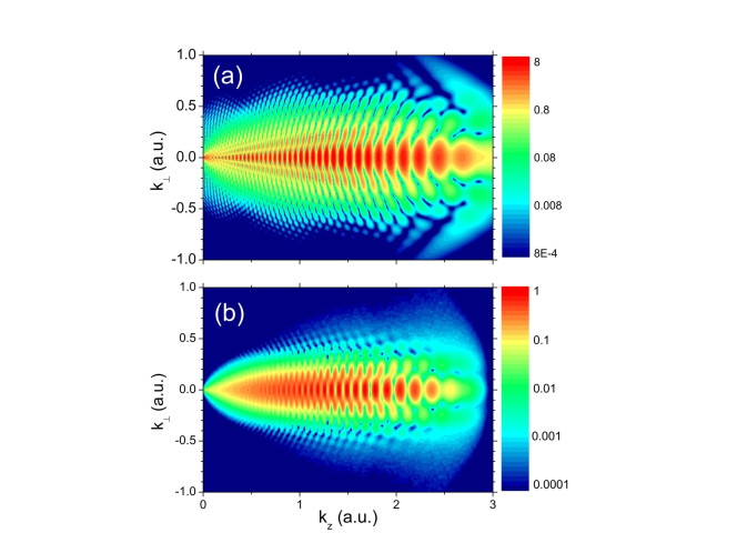
Figure 1: Doubly differential momentum distribution for ionization of atomic hydrogen by the one-cycle sine pulse of Eq. (23) with $F_{0}=0.075,$ $\omega=0.05$ calculated within the (a) TDSE and (b) SCTS.

For the single-cycle electric field of Eq. (23), the simple man’s model (SMM) predicts ionization only in the forward direction, i.e, $0<k_{z}<2F_{0}/\omega$ (see, for example Arbó et al. (2006a)). If one wants to obtain forward-backward symmetrical ionization like in experiments, one needs to use longer electric fields with some ramp on and ramp off. However, we show below that using the single-cycle pulse of Eq. (23) is sufficient to show most of the interference processes characteristic of the electron yield for a more realistic laser pulse. The electron yield after ionization of atomic hydrogen by the electric field in Eq. (23) calculated within the TDSE can be seen in Fig. 1a as a function of the longitudinal momentum $k_{z}$ (along the polarization direction) and transverse momentum $k_{\perp}$ (perpendicular to the polarization direction). The momentum distribution in Fig. 1a spreads mostly along the forward direction and within the classical boundaries predicted by the SMM, i.e., $0<k_{z}<3,$ though extending slightly beyond the classical boundaries due to quantum diffusion. We can see a very rich interference pattern in the quantum momentum distribution. In order to perform the identification of the different kinds of interference present in the complicated interference pattern of Fig. 1a, we also compute the ionization of the hydrogen atom within the SCTS model of Sec. II A using the same electric field of Eq. (23). The SCTS simulation was performed in the four-dimensional phase space $(z,x,v_{0z},v_{x0})$, where $x$ is the component of the position perpendicular to the laser direction. In cylindrical coordinates, we should note that $\rho=|x|.$ We observe that the SCTS distribution in Fig. 1b restricts to the classical boundaries, as expected. We can see that both classical and quantum momentum distributions exhibit a similar interference pattern, although the resemblance is not perfect.

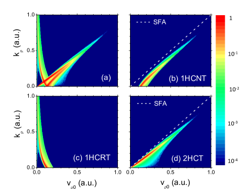
Figure 2: Maps of final perpendicular momentum versus initial perpendicular momentum (right after ionization) for (a) all trajectories, (b) 1HCNT (non-rescattering trajectories ionized during the first half cycle), (c) 1HCRT (rescattering trajectories ionized during the first half cycle), and (d) 2HCT (trajectories ionized during the second half cycle). The dashed line corresponds to the SFA $k_{\rho}=v_{\rho 0}$ prediction. The laser parameters are the same as in Fig. 1.

In order to analyze the different types of electron trajectories present in the ionization process, we show in Fig. 2a the map of asymptotic (final) perpendicular momenta (in cylindrical coordinates) $k_{\rho}=|k_{\perp}|$ versus the momenta at the time of ionization (also in cylindrical coordinates) $v_{0\rho}=|v_{0\perp}|$ calculated for a total of about 20 million trajectories within the CTMC [see Eq. (17)]. Within the SFA, the perpendicular momentum is constant because the action of the ionic potential of the remaining core on the escaping electron is neglected, i.e., $k_{\rho}=v_{\rho 0},$ which is indicated as a dashed line in Figs. 2b and d. Beyond the SFA, electron trajectories can be classified according to the effect of the Coulomb potential on them: (i) weak effect, where the Coulomb potential is not strong enough to change the perpendicular direction of the electron trajectories, i.e., $v_{\perp 0}k_{\perp}>0$, that we call non-rescattering trajectories, also known in the literature as farside trajectories Fuller (1975); Samengo and Barrachina (1996), and (ii) strong effect, where the Coulomb potential is strong enough to change the perpendicular direction of the electron trajectories, i.e., $v_{\perp 0}k_{\perp}<0$, that we call rescattering trajectories, also known in the literature as nearside trajectories Fuller (1975); Samengo and Barrachina (1996). We can see three different regions in the $(k_{\rho},v_{\rho 0})$ map of Fig. 2a. The $(k_{\rho},v_{\rho 0})$ map in Fig. 2b shows only the non-rescattering trajectories ionized during the first half cycle, which we call 1HCNT. One can see very clearly the weak effect of the ionic potential on the escaping trajectories slowing down the electron in the perpendicular direction, i.e., $k_{\perp}<v_{\perp 0}.$ In our case of the hydrogen atom, this effect is called Coulomb focusing, although this name is commonly extended to other atoms with non-Coulombic potentials Kelvich et al. (2016); Daněk et al. (2018a, b). We see that 1HCNT must have an initial transversal momentum higher than a value between $0.1$ a.u. and $0.2$ a.u. for our case. Electron trajectories with less than these values for the initial perpendicular velocity ionized during the first half cycle are strongly affected by the potential of the remaining core changing the sign of the transverse momentum, which can be seen as a collision of the escaping electron with the parent ion. The $(k_{\rho},v_{\rho 0})$ map for this kind of trajectories, that we name 1HCRT, is shown in Fig. 2c. Perpendicular initial velocities are low enough so that the action of the Coulomb potential is strong enough to change the sign of $v_{0x}$ and produce rescattering. We observe that for electron trajectories with low initial transversal momentum (less than $0.1-0.2$ a.u.), the asymptotic transverse momentum $k_{\rho}$ can acquire a very high value compared to the low initial transversal momentum $v_{\rho 0}$ due to the collision event: The lower the initial perpendicular velocity, the higher the final perpendicular velocity. 1HCRT, which are also born during the first half cycle of the pulse, are completely different from the SFA $k_{\rho}=v_{0\rho}$ prediction, as seen in Fig. 2c. The limit of zero perpendicular initial velocity corresponds to a head on collision, so the final perpendicular velocity is high. The limiting case between 1HCNT and 1HCRT corresponds to trajectories which start with a given value of $v_{\rho 0}$ ($0.1\lesssim v_{0\rho}\lesssim 0.2$) and finish with $k_{\rho}=0$, which means that the electrons move asymptotically parallel to the polarization axis in the forward direction. This type of trajectories in the border between rescattered and non-rescattered trajectories is named glory rescattering trajectories Xia et al. (2018). This is equivalent to the problem of the family of orbits encountered when particles are emitted in all directions from a point source in the presence of a Coulomb potential whose center is displaced with respect to the source Samengo and Barrachina (1994).

On the other hand, none of the trajectories released during the second half cycle of the pulse suffer rescattering, i.e., $v_{\perp 0}k_{\perp}>0$ and the corresponding $(k_{\rho},v_{\rho 0}$) map is plotted in Fig. 2d. Due to the same Coulomb focusing effect in the case of 1HCNT, trajectories born during the second half cycle, which we call 2HCT, are weakly affected by the potential of the remaining core and slightly departs from the SFA prediction (dashed line $k_{\rho}=v_{\rho 0}).$ We see from Fig. 2d that 2HCT have a map similar to the SFA $k_{\rho}=v_{0\rho}$ with no rescattering at all. Dislike 1HCNT, there is no lower limit for the initial transverse momentum $v_{\rho 0}$ for 2HCT. Therefore, even for low values of $v_{0\rho}$, the SFA is a good approximation for 2HCT. Summing up, three different types of trajectories are present in the atomic ionization process: 1HCNT ionized during the first half cycle that do not suffer rescattering, 1HCRT ionized during the first half cycle which suffer rescattering, and 2HCT ionized during the 2HC (which do not suffer rescattering).

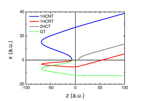
Figure 3: Examples of the three different types of trajectories present in the photoionization process: In blue 1HCNT, in red 1HCRT, and in gray 2HCT. All of these three trajectories have asymptotic momentum $k_{z}=1.5$ a.u. and $k_{\bot}=0.17$. Besides, in dotted line the GT (transition between 1HCNT and 1HCRT, i.e., $k_{\bot}=0$).

In Fig. 3 we show one example for the three different types of electron trajectories 1HCNT, 1HCRT, and 2HCT with the same asymptotic momentum $k_{z}=1.5$ a.u. and $k_{\bot}=0.17$ (corresponding to the first minimum in the holographic structure with longitudinal momentum close to maximum emission according to the SMM). The two trajectories released during the first half cycle 1HCNT and 1HCRT have about the same ionization time (within the statistical uncertainty) $t_{0}=28.02$ a.u. This is a general characteristic for all 1HCNT and 1HCRT. The initial position after the first step (tunneling) depends only on the ionization time and is $z_{0}=-\sqrt{I_{P}/F(t_{0})}=-6.76$ a.u. for both types of trajectories. What makes the difference between the two trajectories 1HCNT and 1HCRT is the initial transverse momentum which is $v_{\bot 0}=0.265$ a.u. for 1HCNT and $v_{\bot 0}=-0.0594$ for the 1HCRT. We can see an abrupt change of direction in the 1HCRT due to the collision with the nucleus when $z\simeq 0$, which changes the direction of the transversal velocity. This collision takes place at $t=149.76$ a.u., which is about $25$ a.u. ( 20 % of an optical cycle) after the end of the electric field ($2\pi/\omega=125.66$ a.u.). The trajectory released within the second half cycle 2HCT starts its trip in the continuum at $t_{0}=90.69$ a.u., which is close to the SMM prediction that the sum of the ionization times for 1HCNT and 2HCT is $2\pi/\omega=125.66$ a.u. The difference stems from the action of the Coulomb potential on the electron trajectories (departing from the SFA). The initial position is $z_{0}=-\sqrt{I_{P}/F(t_{0})}=6.77$, almost the same as the trajectories released during the first half cycle but with the opposite sign due to the inversion of the potential barrier. Finally, we plot an example of a GT with the same asymptotic longitudinal momentum $k_{z}=1.5$ and, by definition, null asymptotic transversal momentum since the collision is not enough to bend the trajectory so that the final transverse momentum has opposite sign to the initial transverse velocity, that in this case is $v_{\bot 0}=-0.126$. There are three different values of the initial perpendicular velocity $v_{0\rho}$ contributing to the electron yield with a particular value of the final momentum $k_{\rho}$ corresponding to the three different types of trajectories.

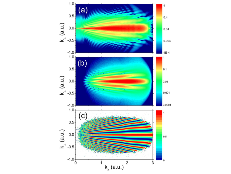
Figure 4: Doubly differential momentum distribution of ionization of atomic hydrogen by the one-cycle sine pulse of Eq. (23) when ionization takes place only during the first half cycle of the pulse (removing ionization during the second half cycle) within (a) the TDSE and (b) the SCTS. (c) SCTS holographic interference pattern $\cos^{2}\left[\left(\Phi_{\mathrm{1HCRT}}-\Phi_{\mathrm{1HCNT}}\right)/2\right]$.

In order to isolate the holographic interference from the imbroglio of quantum interference patterns in Fig. 1a, we artificially switch off the ionization during the second half cycle (2HC) of the pulse by projecting the wave function at the middle of the pulse $\Psi(t=\pi/\omega)$ onto the continuum states dropping out, in this way, the remaining bound states’ populations. The time evolution afterwards ($\pi/\omega<t\leq 2\pi/\omega$) continues normally allowing recapture and further ionization. In this way, only the electron yield ionized during the first half cycle of the pulse and driven by the whole pulse is considered. The corresponding doubly differential momentum distributions can be seen in Fig. 4a. As it can be clearly observed, the well-known holographic structure hindered in Fig. 1a by other types of interferences comes up. This scheme has been recently used for multiple-cycle pulses Xie et al. (2016); López and Arbó (2019); Borbély et al. (2019). In a multiple-cycle pulse, the main lobe centered at $k_{\perp}=0$ flanked by a family of thinner stripes extends also to the backward ($k_{z}<0$) direction. If we exclude ionization during the second half cycle in our semiclassical calculations, only trajectories 1HCNT in Fig. 2b and 1HCRT in Fig. 2c contribute to ionization. The holographic pattern in the doubly differential momentum distribution in Fig. 4b arises as the interference of the two different kinds of electron trajectories: rescattering (1HCRT) and non-rescattering (1HCNT) trajectories ionized during the first half cycle. From a semiclassical perspective, electron trajectories of one kind have a certain accumulated phase [Eq. (12)] from the ionization time up to the final state denoted by a particular momentum $\vec{k}$ in the momentum plane $(k_{z},k_{\perp})$ and interfere with the other kind of trajectories having a different accumulated phase. The similarity of the SCTS (in Fig. 4a) and TDSE (in Fig. 4b) holographic interference pattern is very good. Considering a holographic interference nomenclature, 1HCNT plays the role of the reference beam, whereas 1HCRT does it of the signal beam.

We can enhance the interference pattern calculating the phase of each electron trajectory and average it within every momentum bin in the two-dimensional grid for every electron trajectory type, i.e.,

$$<\Phi_{s}>(k_{zi},k_{\perp j})=\sum_{n}\frac{\Phi_{n}(k_{z},k_{\perp})}{N_{ij}},$$ (24)

where the sum extends over all the $N_{ij}$ electron trajectories with final momentum $k_{zi}-\Delta k_{zi}/2<k_{z}<k_{zi}+\Delta k_{zi}/2,$ and $k_{\perp j}-\Delta k_{\perp j}/2<k_{\perp}<k_{\perp j}+\Delta k_{\perp j}/2$ and the grid $(k_{zi},k_{\perp j})$ span the two-dimensional momentum space. The subscript $s$ denotes the type of electron trajectories, i.e., 1HCRT, 1HCNT, and 2HCT. Then, the interference map is calculated as

$$\cos^{2}\left[\frac{<\Phi_{s}>(k_{zi},k_{\perp j})-<\Phi_{s^{\prime}}>(k_{zi},k_{\perp j})}{2}\right].$$ (25)

In Fig. 4c we show the holographic interference map stemming from the calculation of Eq. (25) for $s=$1HCRT, and $s^{\prime}=$ 1HCNT. The white color corresponds to regions in the $(k_{z},k_{\perp})$ plane with no trajectories of either $s$ or $s^{\prime}$ type. The general shape of the holographic interference pattern in Fig. 4c shows radial stripes with a moderate jump at $k_{z}\simeq 1$ decreasing slightly this value as $k_{\perp}$ increases. The holographic map calculated from Eq. (25) allows to see the interference pattern even for momentum regions where the probability distribution is very low (less than four orders of magnitude lower than the maximum in our case) in Fig. 4c.

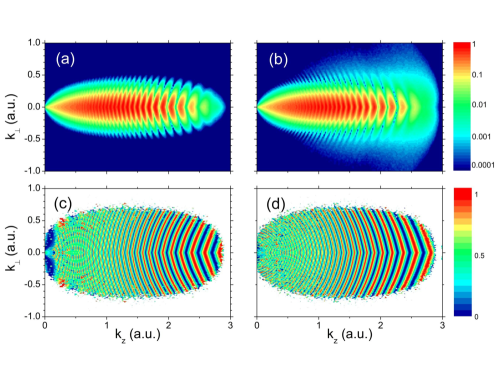
Figure 5: (a) SCTS intracycle interference pattern type I considering only non-rescattering trajectories during the whole pulse doubly differential momentum distribution of ionization of atomic hydrogen. (b) SCTS intracycle interference pattern type II considering direct and rescattered indirect trajectories. (c) Intracycle interference pattern type I $\cos^{2}\left[\left(\Phi_{\mathrm{2HCT}}-\Phi_{\mathrm{1HCNT}}\right)/2\right]$. (d) Intracycle interference pattern type II $\cos^{2}\left[\left(\Phi_{\mathrm{2HCT}}-\Phi_{\mathrm{1HCRT}}\right)/2\right]$. The laser parameters are the same as Fig. 1.

So far, we have analyzed only one type of interference: The holographic interference. On the other hand, two other types of interference naturally come up: the interference between 1HCNT and 2HCT, which we name intracycle type I and is known in the literature as intracycle interference Arbó et al. (2006a, 2012, 2010a), and the interference between 1HCRT and 2HCT, that we name intracycle type II and are scarcely studied in the literature Maxwell and Figueira de Morisson Faria (2018); Maxwell et al. (2018). Fig. 5a shows the results of the intracycle interference type I between 1HCNT and 2HCT as a pattern of convex boomerang-shape stripes centered at the longitudinal momentum axis. The only difference between the intracycle pattern type I of Fig. 5a and the previously studied in the literature Arbó et al. (2006a, 2012, 2010a) is the pointy edge at $k_{\perp}=0$. One can adjudicate the reason of the pointy edge in Fig. 5a to the action of the potential of the remaining core on the escaping electron, which was neglected in previous calculations relying on the strong field approximation Arbó et al. (2006a, 2012, 2010a). We corroborate this result by neglecting the action of the Coulomb potential in our SCTS simulations (not shown). The intracycle interference type II between 1HCRT and 2HCT in Fig. 5b has a similar shape of the intracycle interference type I but the stripes are concave with the pointy edge aiming at the positive $k_{z}$ axis. The respective interference maps of Eq. (25) are shown in Fig. 5c and 5d for the intracycle interferences type I and type II. As in holographic interference, we see how the interference pattern is enhanced in the interference maps for the intracycle interferences type I and II. This fact clearly demonstrates that the stripes in Figs. 5a and 5b stem from the interference of the corresponding types of trajectories. Some odd non-physical moiré patterns can be seen for low parallel momentum because of the plotting method Dran and Arbó (2018).

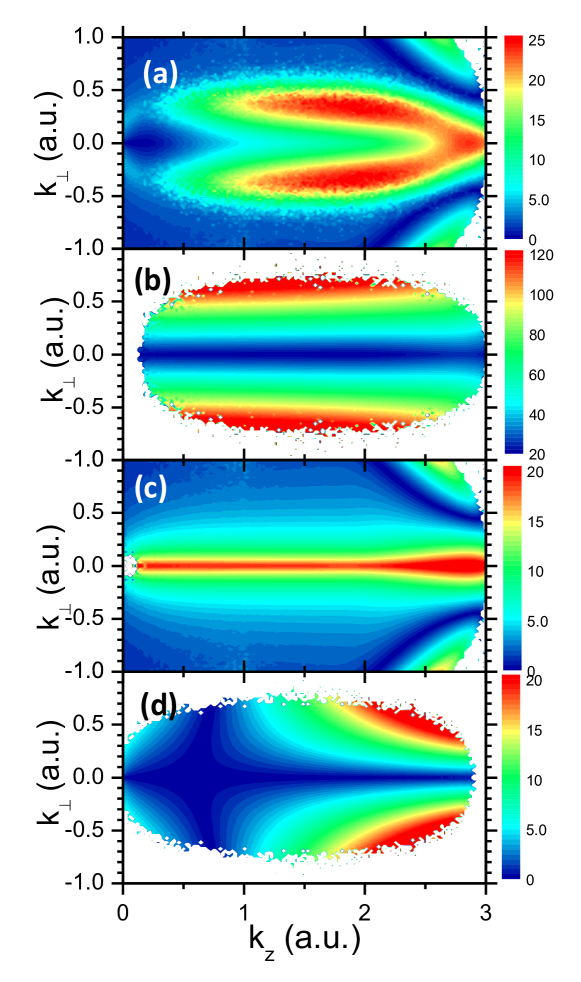
Figure 6: Angular momentum as a function of the transversal and longitudinal momentum. (a) All trajectories, (b) 1HCNT (non-rescattered trajectories ionized during first half cycle), (c) 1HCRT (rescattered trajectories ionized during first half cycle), (d) 2HCT (trajectories ionized during the second half cycle). The laser parameters are the same as in Fig. 1.

As we have seen, the three different types of electron trajectories present in the ionization process situate at essentially the same region (forward emission) in the $(k_{z},k_{\perp})$ momentum plane. Therefore, it is difficult to identify them without tracing back their time evolution. One way to discriminate among the different types of trajectories is looking at their angular momenta. In Fig. 6a, we show the average angular momentum

$$<L>(k_{zi},k_{\perp j})=\sum_{n}\frac{L_{n}(k_{z},k_{\perp})}{N_{i,j}},$$ (26)

where the sum extends over all the electron trajectories with final momentum $k_{zi}-\Delta k_{zi}/2<k_{z}<k_{zi}+\Delta k_{zi}/2,$ and $k_{\perp j}-\Delta k_{\perp j}/2<k_{\perp}<k_{\perp j}+\Delta k_{\perp j}/2$ and the grid $(k_{zi},k_{\perp j})$ spans the two-dimensional momentum space. All the three types of trajectories are present in Fig. 6a. The maximum angular momentum found is about $25$ a.u. in a region similar to a fork bifurcating at the classical edge $k_{z}=3$ a.u. and $k_{\perp}=0$ and aiming backwards. White color corresponds to regions of the final momentum space with no trajectories. We have also performed the same calculation for each of the three types of trajectories separately. In Fig. 6b we plot the angular momentum for 1HCNT as a function of the final momentum $(k_{z},k_{\perp}).$ We see that the minimum angular momentum for 1HCNT is at $k_{\perp}=0$ and $<L>$ increases from $20$ a.u. with the absolute value of the perpendicular velocity $k_{\rho}=|k_{\perp}|$ reaching very high values close to $120$ a.u. at the classical boundaries. The angular momentum of 1HCRT in Fig. 6c exhibits a completely different behavior: The maximum corresponds to $<L>=20$ a.u. and the angular momentum decreases with the absolute value of the perpendicular velocity $k_{\rho}=|k_{\perp}|.$ Therefore, we can say that 1HCNT and 1HCRT have different values of angular momentum, coinciding only for $k_{\perp}=0$. In fact, this is the same result pointed out in the description of Fig. 2b and 2c because the definition of rescattering and non-rescattering trajectories mixes when $k_{\rho}=k_{\perp}=0,$ corresponding to the rescattering glory trajectories described before. Coming back to the analysis of the angular momentum, we see in Fig. 2c that 2HCT have angular momentum with a minimum at $k_{\perp}=0$ but, in contrast to the trajectories ionized during the 1HC, the minimum value is $<L>=0$.

The angular momentum distribution of the electron yield has been calculated at the end of the pulse, i.e., $t=2\pi/\omega$, which is the same at the asymptotic detection time $t\rightarrow\infty$ since the angular momentum is a constant of motion once the laser pulse has been switched off. In Fig. 7a, we show the quantum angular momentum distribution after the end of the pulse (calculated within the TDSE). The distribution shows a sharp peak at very low angular momenta with a broad plateau with maximum at $L\simeq 25$ a.u. slowly decreasing up to $L\approx 100$ a.u. In order to analyze the reason of this shape, we also perform the quantum calculation of the momentum distribution for ionization during the first half cycle, which exhibits a very broad distribution with a maximum value at $L\simeq 28$ in Fig. 1. Therefore, we can conclude that the sharp peak at very low angular momenta stems from ionization during the second half of the pulse.

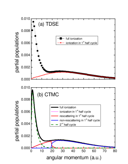
Figure 7: Angular momentum distribution for the different kinds of trajectorie. (a) TDSE calculations and (b) CTMC calculations. The laser parameters are the same as in Fig. 1.

In order to corroborate this, we calculate the classical angular momentum distribution [calculated within the CTMC with Eq. (17)] for each of the three types of electron trajectories present in the ionization process. We observe in Fig. 7b that the sharp peak at low momenta is due almost exclusively by the contribution of 2HCT, that is, the electron trajectories born during the second half cycle (which do not suffer rescattering). In turn, 1HCNT (which do not suffer rescattering either) contributes to the broad plateau only for angular momentum $L\gtrsim 20$ a.u., as previously shown in Fig. 2b. Trajectories released within the first half cycle ending with lower angular momentum ($L\lesssim 20$ a.u.) suffer rescattering (1HCRT), contributing to the lower region of the plateau and very little to the sharp peak at low angular momentum. However, the low energy peak of the TDSE momentum distribution in Fig. 7a is slightly broader than the corresponding CTMC in Fig. 7b. The sum of the CTMC 1HCRT and 1HCNT contributions shown in Fig. 7c is very similar to the quantum distribution with ionization only during the first half cycle. We can see a very high quantum classical correspondence for the angular momentum, even though the resemblance between the quantum and classical results is not perfect.

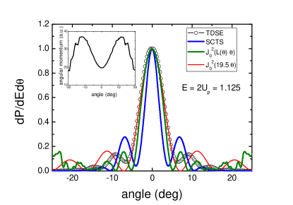
Figure 8: Doubly differential angle-energy distribution as a function of the emission angle for fix energy $E=1.125$ a.u. Calculations are performed with different methods: dots correspond to TDSE, thick blue line to SCTS, green line to the square of the Bessel function of the angle-dependent angular momentum $L(\theta)$ times the angle $\theta,$ and thin red line is the same but replacing $L(\theta)$ by $L(0)=19.5.$ The inset displays the function $L(\theta)$ calculated at $E=1.125$ a.u. The laser parameters are the same as in Fig. 1. All the functions are normalized to unity at forward direction ($\theta=0^{\circ}$)

For the sake of a quantitative comparison between the SCTS and TDSE calculations, In Fig. 8 we plot the SCTS and TDSE doubly differential energy-angle distribution as a function of the emission angle for a fix energy $E=2U_{p}=1.125$ a.u. (corresponding to a momentum $k=1.5$ a.u., close to the maximum of the energy distribution). We observe that the general shape of the semiclassical and quantum distributions are similar with a central peak at forward emission ($\theta=0^{\circ}$) and symmetrical lower peaks at both sides. Despite this qualitative similarity, several differences are observed. Firstly, the central peak of the SCTS distribution is narrower than the quantum one. In this sense, the first minima of the TDSE distribution are at $\theta\simeq\pm 6.5^{\circ},$ whereas the corresponding SCTS ones are situated at $\theta=\pm 4^{\circ}.$ Besides, the position of the first peaks of the TDSE distribution is at $\theta\simeq\pm 9^{\circ}$ with a height of $0.135$ relative to the central peak (normalized in the figure) whereas the corresponding SCTS ones lie at $\theta\simeq\pm 7^{\circ}$ with height of $0.28.$ According to Eq. (22) in Sec. II, due to an interference process of glory trajectories, the angular distribution (for a fix energy) can be described by the square of a Bessel function of the first type of the angular momentum times the angle, i.e., $J_{0}^{2}(L\ \theta)$ (see Ref. Xia et al. (2018)). Therefore, in the inset of Fig. 8 we show the SCTS angular momentum $L(\theta)$ as a function of the angle for the same fix energy $E=1.125$ a.u. The value of the angular momentum at zero emission angle ($\theta=0^{\circ}$) is $L(0^{\circ})=19.5$ a.u., then it increases as the emission angle departs from the forward emission up to $|\theta|\simeq 12^{\circ}$ where it reaches the maximum angular momentum and then decreases as the emission angle increases further $|\theta|\simeq 12^{\circ}$. In a thin red line we show that $J_{0}^{2}(L(0^{\circ})\ \theta)$ follows the TDSE distribution very accurately for low emission angles, i.e., $|\theta|\lesssim 6^{\circ}$ but then it predicts angles of minima and maxima higher than the quantum simulation. If we replace the constant value of $L(0^{\circ})$ by the function $L(\theta)$ into the Bessel function, the prediction $J_{0}^{2}(L(\theta)\ \theta)$ changes considerably. It departs from the SCTS at lower angles $|\theta|\simeq 3^{\circ}$ with first maxima at $|\theta|\simeq 7^{\circ},$ very close to the semiclassical prediction, although higher order peaks set off from the SCTS.

IV Conclusions

We have studied the interference phenomena in atomic ionization by a single-cycle laser pulse. We have shown that the SCTS qualitatively reproduces the quantum results. Within the SCTS model we have identified three different types of electron trajectories with three different types of interferences. Non-rescattering trajectories (1HCNT) and rescattering trajectories (1HCRT) lead to the well-known holographic interference pattern in the doubly differential momentum distribution. We have shown that one way to distinguish between these two types of trajectories (1HCNT and 1HCRT) is through their different final angular momentum. We have revisited the glory rescattering theory of Ref. Xia et al. (2018) and found that it qualitatively explains the TDSE holographic interference pattern but some quantitative discrepancies arise. Moreover, glory trajectories ($k_{\perp}\simeq 0$) are in the transition between non-rescattering trajectories 1HCNT (where $k_{\perp}v_{x0}>0$) and rescattering trajectories 1HCRT (where $k_{\perp}v_{x0}<0$). For this reason, we have dropped out the name “rescattering” used in Ref. Xia et al. (2018) and just call them glory trajectories.

Electron trajectories born during the second half cycle 2HCT do not suffer rescattering and interfere with the other two types of trajectories (released during the first half cycle). On one hand, the interference between 2HCT and 1HCNT gives rise to the well-known intracycle interference type I Chirila and Potvliege (2005); Arbó et al. (2006b, a). The intracycle type I interference calculated within the SCTS exhibits a family of convex pointy stripes in the doubly differential momentum distribution. On the other hand, the interference between 2HCT and 1HCRT gives rise to the intracycle interference type II as a family of concave pointy stripes in the momentum distribution. Whereas the wedges of the stripes of the interference type I aim to the backward direction, those corresponding to interference type II do it forwards. The sharp wedges at $k_{\perp}=0$ for both intracycle interferences type I and II are due to the effect of the Coulomb potential with the escaping electron and is not present in previous calculations based on the SFA Chirila and Potvliege (2005); Arbó et al. (2006b, a).

Finally, we have shown both quantum mechanically and classically that the very sharp peak at low angular momentum in the angular momentum distribution mostly stems from ionization during the second half cycle, whereas ionization during the first half cycle contributes to the very broad plateau reaching high values of the angular momentum up to $L\sim 100$.