Relaxation of One-dimensional Collisionless Gravitating Systems

Abstract

In an effort to better understand collisionless relaxation processes in gravitational systems, we investigate one-dimensional models. Taking advantage of a Hermite-Legendre expansion of relevant distribution functions, we present analytical and numerical behaviors of Maxwell-Boltzmann entropy. In particular, we modestly perturb systems about a separable-solution equilibrium and observe their collisionless evolution to a steady state. We verify the time-independence of fine-grained entropy in these systems before turning our attention to the behavior of coarse-grained entropy. We also verify that there is no analogue to the collisional H-theorem for these systems. Competing terms in the second-order coarse-grained entropy make it impossible to guarantee continuously increasing entropy. However, over dynamical time-scales the coarse-grained entropy generally increases, with small oscillations occurring. The lack of substantive differences between the entropies in test-particle and self-gravitating cases suggests that phase mixing, rather than violent relaxation associated with potential changes, more significantly drives the coarse-grained entropy evolution. The effects of violent relaxation can be better quantified through analysis of energy distributions rather than phase-space distributions.

1 Introduction

Thermodynamics of self-gravitating collisionless systems is an interesting subject. In three-dimensions, such systems do not have thermodynamic equilibria, characterized by a constant kinetic temperature or a maximum entropy (e.g. Binney & Tremaine, 1987, §4.7). Investigations of statistical mechanics and thermodynamic approaches to understanding the mechanical equilibria of self-gravitating systems have a long history. A succinct introduction to the problem and historical review of progress made is given by Levin et al. (2014).

In this work, we take on a related, but simpler, situation. One-dimensional self-gravitating systems can be thought of either as particles interacting in one-dimension through a distance-independent force or as infinite sheets of mass in three-dimensions. Collisionless versions of these systems do have equilibria with simple, separable forms (Camm, 1950). In fact, the separable equilibrium distribution function has Boltzmann form. Readers interested in the nature of this equilibrium and its relationship to statistical equilibria in the microcanonical and canonical ensembles may find previous work by Rybicki (1971) and Joyce & Worrakitpoonpon (2010) particularly interesting. The temperature of such an equilibrium can be connected to an energy scaling factor, as in normal collisional gas situations. Additionally, the kinetic and thermal temperatures $kT=1/\beta$ are identical for these equilibria.

Our goal is to understand collisionless relaxation from an initial state that is perturbed from this equilibrium, which we pursue by investigating the behavior of Maxwell-Boltzmann entropy. Based on the work of Tremaine, Hénon, & Lynden-Bell (Tremaine et al.1986), we use the Maxwell-Boltzmann qualifier here to specify the common form of the entropy function we will deal with. On a side note, we have also confirmed that the Lynden-Bell entropy (Lynden-Bell, 1967; Barnes & Williams, 2012) behaves essentially identically to the Maxwell-Boltzmann entropy in these non-degenerate systems. For simplicity, we will assume the reader implicitly inserts the Maxwell-Boltzmann qualifier to all further references to entropy. We investigate how well the Tremaine et al. analogy to the collisional H-theorem (guaranteeing that entropy increases during relaxation) explains aspects of the dynamics of these systems. We also compare the evolutions of systems composed of test particles to self-gravitating situations in an attempt to separate the influences of phase mixing and violent relaxation.

Phase mixing describes evolution in which any occupied region of phase space tends to mix with unoccupied phase space, producing a lower average phase-space density. Particle interactions are not necessary for phase mixing to occur. Violent relaxation, on the other hand, generally results when the dynamics of a system are driven by a time-dependent potential (Lynden-Bell, 1967). In our simulations, violent relaxation is driven by self-gravitation in systems that are in non-stationary states. In general, phase mixing occurs in all of our simulated systems, test-particle and self-gravitating, but violent relaxation is absent from test-particle situations.

While we do use $N$-body simulations, the basis of our analysis takes advantage of a Hermite-Legendre decomposition of distribution functions. This effectively changes the problem from one involving continuous phase-space coordinates to a discrete coefficient space situation. The dynamics of an evolving system with infinite range forces then reduces to a local interaction between coefficients. The basics of this approach are presented in Barnes & Ragan (2014). We will expand upon the arbitrary perturbation discussion in Ragan & Barnes (2019) when dealing with second-order effects in what follows.

The introduction to essential features of our approach (coefficient dynamics and second-order perturbation theory) is provided in the discussion of energy given in § 2. The entropy analysis for both fine- and coarse-grained situations follows in Section 3. We also highlight agreement between our coefficient results and a thermodynamical approach to calculating entropy changes. The importance of energy distributions, as opposed to entropy, in quantifying violent relaxation is explored in Section 4. Our approach and results are summarized in § 5.

2 Energy

2.1 General Relationships

For a one-dimensional situation, phase space is simply a position-velocity plane $(x,v)$. We adopt dimensionless versions of position and velocity using system mass $M$, gravitational coupling constant $g$, and an energy scale $\beta$. Specifically,

$$\chi=\frac{\beta gM}{2}x\quad\mbox{and}\quad\varpi=\sqrt{\frac{\beta}{2}}v.$$

The dimensionless time is then defined by

$$\tau=\sqrt{\frac{\beta}{2}}gMt.$$

We adopt these dimensionless coordinates for the remainder of this paper.

For any distribution function $f(\chi,\varpi)$, we define the dimensionless mass density function as,

$$\Lambda=\int_{-\infty}^{\infty}f\,\mathrm{d}\varpi.$$ (1)

We also define the dimensionless one-dimensional self-gravitating acceleration as,

$$\alpha=\frac{a}{gM}=-\int_{-\infty}^{\chi}\Lambda(\chi^{\prime})\,\mathrm{d}\chi^{\prime}+\int_{\chi}^{\infty}\Lambda(\chi^{\prime})\,\mathrm{d}\chi^{\prime}.$$ (2)

Consider a distribution function decomposition in terms of Hermite and Legendre polynomials,

$$f(\chi^{\prime\prime},\varpi)=\sum_{m,n=0}^{\infty}C_{m,n}H_{m}(\varpi)P_{n}(\chi^{\prime\prime})\operatorname{sech}^{2}\chi^{\prime\prime}e^{-\varpi^{2}}.$$ (3)

We note that the coefficients in this decomposition are modified from those in Barnes & Ragan (2014) and Ragan & Barnes (2019). The coefficients here have absorbed factors of $\sqrt{(2n+1)/2}$ and $1/\sqrt{2^{m}\sqrt{\pi}m!}$. With this choice we have that,

$$\Lambda=\sqrt{\pi}\sum_{n=0}^{\infty}C_{0,n}P_{n}\operatorname{sech}^{2}\chi^{\prime\prime},$$ (4)

where we have taken advantage of the orthogonality relations for Hermite polynomials,

$$\int_{-\infty}^{\infty}H_{j}(\varpi)H_{k}(\varpi)\,\mathrm{d}\varpi=2^{j}\sqrt{\pi}j!\,\delta_{jk},$$

where $\delta$ is the Kronecker delta. With this density (Equation 4), the acceleration becomes,

$$\alpha=\sqrt{\pi}\sum_{n=0}^{\infty}C_{0,n}\left[\int_{\tanh\chi^{\prime}}^{1}P_{n}(u)\,\mathrm{d}u-\int_{-1}^{\tanh\chi^{\prime}}P_{n}(u)\,\mathrm{d}u\right],$$ (5)

where we have made the substitution $u=\tanh\chi$. These integrals may be carried out to produce an expression for acceleration purely in terms of Legendre polynomials,

$$\alpha=-2\sqrt{\pi}\sum_{n\geq 0}\frac{C_{0,n}}{2n+1}\left[P_{n+1}(\tanh\chi^{\prime})-P_{n-1}(\tanh\chi^{\prime})\right].$$ (6)

The dimensionless potential function may now be written as,

$$\Phi(\chi)-\Phi(0) = 4\sqrt{\pi}\sum_{n\geq 0}\frac{C_{0,n}}{2n+1}\left[\int_{0}^{\chi}P_{n+1}(\tanh\chi^{\prime})\,\mathrm{d}\chi^{\prime}-\right.$$ (7)

$$\left.\int_{0}^{\chi}P_{n-1}(\tanh\chi^{\prime})\,\mathrm{d}\chi^{\prime}\right].$$

Again taking advantage of the substitution $u=\tanh\chi$, the integrals may be combined into,

$$\int_{0}^{\tanh\chi}\frac{P_{n+1}(u)-P_{n-1}(u)}{1-u^{2}}\,\mathrm{d}u.$$ (8)

Using that

$$\frac{\mathrm{d}P_{N}}{\mathrm{d}u}=\frac{N}{1-u^{2}}(P_{N-1}-uP_{N}),$$

and

$$uP_{N}=\frac{N+1}{2N+1}P_{N+1}+\frac{N}{2N+1}P_{N-1},$$

one can show that Equation 8 reduces to

$$-\frac{2n+1}{n(n+1)}\left[P_{n}(\tanh\chi)-P_{n}(0)\right],$$ (9)

for $n>0$. When $n=0$, Equation 8 is simply $\ln{(\cosh\chi)}$. Using the fact that $P_{n}(0)$ is zero for odd $n$ and demanding that $\lim_{\chi\rightarrow\infty}\Phi=2\chi$ (system mass has finite extent) leads to,

$$\Phi(\chi)=2\ln{(2\cosh\chi)}+4\sqrt{\pi}\sum_{n\geq 1}\frac{C_{0,n}}{n(n+1)}\left[1-P_{n}(\tanh\chi)\right].$$ (10)

With this expression and Equation 3, the dimensionless potential energy of the system may be written as,

$$U = \frac{1}{2}\int_{-\infty}^{\infty}\int_{-\infty}^{\infty}f\Phi\,\mathrm{d}\chi\mathrm{d}\varpi$$ (11)

$$= 1+2\sqrt{\pi}\sum_{n\geq 1\atop{\rm odd}}\frac{C_{0,n}}{n(n+1)}+4\sqrt{\pi}\sum_{n\geq 2\atop{\rm even}}\frac{C_{0,n}}{n(n+1)}-$$

$$4\pi\sum_{n\geq 1}\frac{C_{0,n}^{2}}{n(n+1)(2n+1)}.$$

Given that the dimensionless kinetic energy can be expressed as (Barnes & Ragan, 2014),

$$K = \int_{-\infty}^{\infty}\int_{-\infty}^{\infty}f\varpi^{2}\,\mathrm{d}\chi\mathrm{d}\varpi$$ (12)

$$= \sqrt{\pi}(C_{0,0}+4C_{2,0})$$

$$= \frac{1}{2}+4\sqrt{\pi}C_{2,0},$$

the Hermite-Legendre decomposition provides an interesting picture of energy behavior in these systems in ($m,n$) coefficient space. In linear perturbation regimes, coefficient dynamics equations demand that only diagonally neighboring coefficients can interact (Barnes & Ragan, 2014). In this way, kinetic energy changes always link directly to large-spatial-scale variations in the potential ($m=0,n=2$ in Equation 10) which then propagate to smaller-spatial-scale potential variations with larger $n$. This energy flow to higher $n$ coefficients passes through $m=1$ terms, which have to act as conduits, as they cannot directly contribute to the total energy.

2.2 Perturbation Analysis

As mentioned above, the dynamics of the system can be written in terms of decomposition coefficients if the perturbation strength is kept small. The original coefficient evolution investigation in Barnes & Ragan (2014) only included first-order terms. However, from the general potential energy expression above, one can see that complete potential energy calculations require second-order terms. As we are interested in capturing violent relaxation processes involving potential changes, we need to extend our perturbation analysis to second-order as well.

This leads us to consider systems such that the distribution function can be written as,

$$f=f_{0}+\epsilon f_{1}+\epsilon^{2}f_{2},$$ (13)

where

$$f_{0}=\frac{1}{2\sqrt{\pi}}\operatorname{sech}^{2}\chi e^{-\varpi^{2}}$$

describes the separable-solution equilibrium (hereafter, separable equilibrium for brevity) and $\epsilon^{2}\ll 1$. The perturbation functions have similar forms,

$$f_{1}=\sum_{m,n\atop m\neq n=0}c_{m,n}H_{m}(\varpi)P_{n}(\tanh\chi)\operatorname{sech}^{2}\chi e^{-\varpi^{2}},$$ (14)

and

$$f_{2}=\sum_{m,n\atop m\neq n=0}d_{m,n}H_{m}(\varpi)P_{n}(\tanh\chi)\operatorname{sech}^{2}\chi e^{-\varpi^{2}},$$ (15)

where the $m=n=0$ terms are explicitly excluded.

Using the results of the previous section, we calculate the dimensionless energy of our system as,

$$E=K+U=\int_{-\infty}^{\infty}\int_{-\infty}^{\infty}f\varpi^{2}\,\mathrm{d}\chi\mathrm{d}\varpi+\frac{1}{2}\int_{-\infty}^{\infty}\int_{-\infty}^{\infty}f\Phi\,\mathrm{d}\chi\mathrm{d}\varpi.$$ (16)

To second order, the kinetic energy term is,

$$K = K_{0}+\epsilon K_{1}+\epsilon^{2}K_{2}$$ (17)

$$= \iint f_{0}\varpi^{2}\,\mathrm{d}\chi\mathrm{d}\varpi+\epsilon\iint f_{1}\varpi^{2}\,\mathrm{d}\chi\mathrm{d}\varpi+$$

$$\epsilon^{2}\iint f_{2}\varpi^{2}\,\mathrm{d}\chi\mathrm{d}\varpi.$$

From here on, infinite limits of integration should be assumed wherever limits are omitted. Completing these integrations produces,

$$K_{0} = \frac{1}{2},$$ (18)

$$K_{1} = 4\sqrt{\pi}c_{2,0},\quad\mbox{and}$$

$$K_{2} = 4\sqrt{\pi}d_{2,0}.$$

The potential energy contribution is,

$$U = U_{0}+\epsilon U_{1}+\epsilon^{2}U_{2}=$$ (19)

$$\frac{1}{2}\iint f_{0}\Phi_{0}\,\mathrm{d}\chi\mathrm{d}\varpi+\frac{\epsilon}{2}\iint(f_{1}\Phi_{0}+f_{0}\Phi_{1})\,\mathrm{d}\chi\mathrm{d}\varpi+$$

$$\frac{\epsilon^{2}}{2}\iint(f_{2}\Phi_{0}+f_{1}\Phi_{1}+f_{0}\Phi_{2})\,\mathrm{d}\chi\mathrm{d}\varpi,$$

where the infinite limits of integration are assumed. Here, $\Phi_{0}=2\ln{(2\cosh\chi)}$ and,

$$\Phi_{1}=4\sqrt{\pi}\sum_{n\geq 1}\frac{c_{0,n}}{n(n+1)}\left[1-P_{n}(\tanh\chi)\right],$$

and

$$\Phi_{2}=4\sqrt{\pi}\sum_{n\geq 1}\frac{d_{0,n}}{n(n+1)}\left[1-P_{n}(\tanh\chi)\right].$$

We now write the energy of the system as,

$$E=E_{0}+\epsilon E_{1}+\epsilon^{2}E_{2},$$ (20)

where

$$E_{0} = \frac{3}{2},$$ (21)

$$E_{1} = 4\sqrt{\pi}\left[c_{2,0}+\sum_{n\geq 2\atop{\rm even}}\frac{c_{0,n}}{n(n+1)}+\frac{1}{2}\sum_{n\geq 1\atop{\rm odd}}\frac{c_{0,n}}{n(n+1)}\right],\,\mbox{and}$$

$$E_{2} = 4\sqrt{\pi}\left[d_{2,0}+\sum_{n\geq 2\atop{\rm even}}\frac{d_{0,n}}{n(n+1)}+\frac{1}{2}\sum_{n\geq 1\atop{\rm odd}}\frac{d_{0,n}}{n(n+1)}\right]-$$

$$4\pi\sum_{n\geq 1}\frac{c_{0,n}^{2}}{n(n+1)(2n+1)}.$$

The terms in the square brackets in each of these expressions reflect the interaction of the perturbation with the equilibrium, but the term proportional to $c_{0,n}^{2}$ in the second-order energy is due to the perturbation interacting with itself. Its origin lies with the $f_{1}\Phi_{1}$ term in Equation 19.

Energy must be conserved in these systems, but in order to prove this we need dynamics equations for the first- and second-order coefficients $\dot{c}_{m,n}$ and $\dot{d}_{m,n}$. The details of the derivation of the first-order coefficient equation have been presented in Barnes & Ragan (2014). The second-order coefficient equation closely follows that discussion, but there is an interesting addition. We find that,

$$\dot{d}_{m,n}=$$

$$L_{m,n}^{m-1,n-1}\,d_{m-1,n-1}+L_{m,n}^{m-1,n+1}\,d_{m-1,n+1}+$$

$$L_{m,n}^{m+1,n-1}\,d_{m+1,n-1}+L_{m,n}^{m+1,n+1}\,d_{m+1,n+1}-R_{m,n},$$

where the matrix elements $L_{m,n}^{i,j}$ are given by

$$L_{m,n}^{m-1,n-1} = \frac{n(n-1)-2\delta_{1,m}}{2(2n-1)},$$

$$L_{m,n}^{m-1,n+1} = -\frac{(n+1)(n+2)-2\delta_{1,m}}{2(2n+3)},$$

$$L_{m,n}^{m+1,n-1} = \frac{(m+1)n(n+1)}{2n-1},$$

$$L_{m,n}^{m+1,n+1} = -\frac{(m+1)n(n+1)}{2n+3},$$ (23)

where $m,n,i,j\geq 0$. The Kronecker delta functions are present for self-gravitating systems only. Test-particle systems do not require them to determine their dynamics. Replacing $d$ with $c$ and setting $R_{m,n}=0$ in Equation 2.2 provides the coefficient dynamics for the first-order perturbation. The additional term for the second-order is given by,

$$R_{m,n} = 2\sqrt{\pi}(2n+1)\sum_{p\geq 1}\frac{c_{0,p}}{2p+1}\left\{c_{m-1,0}Q_{n+p+1}^{(n,p+1)}+\right.$$ (24)

$$\sum_{s=0\atop{\rm even}}^{n+p-1}\left[Q_{s}^{(n,p+1)}\left(\frac{c_{m-1,n+p+1-s}}{2(n+p+1-s)+1}\right)-\right.$$

$$\left.\left.Q_{s}^{(n,p-1)}\left(\frac{c_{m-1,n+p-1-s}}{2(n+p-1-s)+1}\right)\right]\right\}.$$

The $Q$ functions arise from writing products of Legendre polynomials as series of single Legendre polynomials and are defined by (Dougall, 1953),

$$Q_{s}^{(j,k)}=\frac{2j+2k-2s+1}{2j+2k-s+1}\frac{\lambda_{s/2}\lambda_{j-s/2}\lambda_{k-s/2}}{\lambda_{j+k-s/2}},$$

where

$$\lambda_{B}=\frac{(2B)!}{2^{B}(B!)^{2}},$$

if $B\geq 0$ and is zero otherwise.

We will focus on a discussion of the time-derivative of $E_{2}$. In this discussion, we will assume that all even-$m$, odd-$n$ coefficients are zero. This guarantees that the system center-of-mass position and velocity are constants. From Equation 21,

$$\dot{E}_{2} = 4\sqrt{\pi}\left[\dot{d}_{2,0}+\sum_{n\geq 2\atop{\rm even}}\frac{\dot{d}_{0,n}}{n(n+1)}\right]-$$ (25)

$$4\pi\frac{\partial}{\partial\tau}\left[\sum_{n\geq 1}\frac{c_{0,n}^{2}}{n(n+1)(2n+1)}\right].$$

Using Equation 2.2 and the specific values of $Q$, one can show that,

$$\dot{d}_{2,0}+\sum_{n\geq 2\atop{\rm even}}\frac{\dot{d}_{0,n}}{n(n+1)}=-2\sqrt{\pi}\sum_{n\geq 1}\frac{c_{0,n}}{2n+1}\left[\frac{c_{1,n+1}}{2n+3}-\frac{c_{1,n-1}}{2n-1}\right].$$ (26)

The term in square brackets on the right-hand side of this expression can be re-cast using the first-order version of Equation 2.2 (with $R_{m,n}=0$). We have that,

$$\frac{\dot{c}_{0,n}}{n(n+1)}=\frac{c_{1,n-1}}{2n-1}-\frac{c_{1,n+1}}{2n+3}.$$ (27)

Substituting this relation into Equation 26 results in,

$$\dot{d}_{2,0}+\sum_{n\geq 2\atop{\rm even}}\frac{\dot{d}_{0,n}}{n(n+1)}=\sqrt{\pi}\frac{\partial}{\partial\tau}\left[\sum_{n\geq 1}\frac{c_{0,n}^{2}}{n(n+1)(2n+1)}\right].$$ (28)

Using this expression in Equation 25 provides us with the proof that the second-order energy is time-independent. The proof for the first-order energy is simpler, as the first-order version of Equation 25 does not include the last term. It is then straightforward to show from the first-order coefficient dynamics equations that,

$$\dot{c}_{2,0}+\sum_{n\geq 2\atop{\rm even}}\frac{\dot{c}_{0,n}}{n(n+1)}=0.$$ (29)

3 Entropy

In a collisional system, the H-theorem guarantees that entropy increases as a system approaches equilibrium. For collisionless systems, (Tremaine et al.1986) have shown that any convex function of the distribution function, like the Maxwell-Boltzmann entropy, will not decrease during relaxation. In our discussion, we are careful to distinguish between entropy based on the fine-grained distribution function and entropy based on a coarse-grained distribution function. In a collisionless system, the fine-grained entropy is a conserved quantity, like energy. A coarse-grained entropy does not have to be conserved, and we are interested in how its evolution compares to the Tremaine et al. collisionless H-theorem prediction. Our goal in this section is to derive and understand a perturbation expression of the fine-grained entropy and to investigate the behavior of coarse-grained entropy.

3.1 Fine-grained Entropy

We use the standard expression for Maxwell-Boltzmann entropy,

$$s=-\int\int f\ln{f}\,\mathrm{d}\chi\mathrm{d}\varpi.$$ (30)

As mentioned previously, we have also utilized a Lynden-Bell entropy. As our situations are not degenerate, there is essentially no difference between values derived from the two approaches, and we will simply refer to entropy in this discussion. Using the perturbation expansion in Equation 13 allows us to write the fine-grained entropy to second-order as,

$$s=s_{0}+\epsilon s_{1}+\epsilon^{2}s_{2}=$$ (32)

$$-\iint f_{0}\ln{f_{0}}\,\mathrm{d}\chi\mathrm{d}\varpi-\epsilon\iint f_{1}(1+\ln{f_{0}})\,\mathrm{d}\chi\mathrm{d}\varpi-$$

$$\epsilon^{2}\iint\left[f_{2}(1+\ln{f_{0}})+\frac{f_{1}^{2}}{2f_{0}}\right]\,\mathrm{d}\chi\mathrm{d}\varpi.$$

Due to the Boltzmann form of equilibrium, we have that

$$\ln{f_{0}}=-\ln{(2\sqrt{\pi})}-e_{0}=-\ln{(2\sqrt{\pi})}-\varpi^{2}-2\ln{(2\cosh{\chi})},$$ (33)

where $e$ is the dimensionless energy per unit mass. In order to complete the integrations, we need to take advantage of the fact that,

$$\int_{-\infty}^{\infty}P_{n}(\tanh\chi)\ln{(\cosh\chi)}\operatorname{sech}^{2}\,\mathrm{d}\chi=$$

$$-\frac{1}{2}\int_{-1}^{1}P_{n}(u)\ln{(1-u^{2})}\,\mathrm{d}u=\left\{\begin{array}[]{l}2(1-\ln{2}),\,\mbox{for $n=0$}\\ \frac{2}{n(n+1)},\,\mbox{for $n\geq 2$, even.}\end{array}\right.$$

The zeroth-, first-, and second-order fine-grained entropy expressions can be written as,

$$s_{0} = \ln{(2\sqrt{\pi})}+\frac{5}{2},$$

$$s_{1} = 4\sqrt{\pi}\left[c_{2,0}+\sum_{n\geq 2\atop{\rm even}}\frac{c_{0,n}}{n(n+1)}\right],$$ (35)

$$s_{2} = 4\sqrt{\pi}\left[d_{2,0}+\sum_{n\geq 2\atop{\rm even}}\frac{d_{0,n}}{n(n+1)}\right]-2\pi\sum_{m,n\atop m\neq n=0}\frac{2^{m}m!}{2n+1}c_{m,n}^{2}.$$

The first expression in Equation 3.1 is trivially time-independent, and $\dot{s}_{1}=0$ because that term is the same as the first-order energy (ignoring the even-odd coefficients), which is time-independent. We note that final term in the $s_{2}$ expression shows that any first-order perturbation (all $d_{m,n}=0$) results in a reduction in entropy. As long as the perturbation imparts no first-order energy ($E_{1}=s_{1}=0$), the separable equilibrium is also the maximum entropy state.

To show that $\dot{s}_{2}=0$, we use Equation 26 to write,

$$\dot{s}_{2} = -8\pi\sum_{n\geq 1}\frac{c_{0,n}}{2n+1}\left[\frac{c_{1,n+1}}{2n+3}-\frac{c_{1,n-1}}{2n-1}\right]-$$ (36)

$$4\pi\sum_{m,n\atop m\neq n=0}\frac{2^{m}m!}{2n+1}c_{m,n}\dot{c}_{m,n}.$$

We focus our attention on the second right-hand-side term. Using the first-order coefficient dynamics equations, we see that these $c_{m,n}\dot{c}_{m,n}$ terms behave just like coefficients in the test-particle case, except for $m=1$. The rightmost term in Equation 36 can be re-cast as,

$$\sum_{m,n\atop m\neq n=0}\frac{2^{m}m!}{2n+1}c_{m,n}\dot{c}_{m,n}=\sum_{m,n\atop m\neq n=0}\frac{2^{m}m!}{2n+1}c_{m,n}^{\rm test}\dot{c}_{m,n}^{\rm test}-$$ (37)

$$\sum_{n\geq 0}\frac{2c_{1,n}}{2n+1}\left[\frac{c_{0,n-1}}{2n-1}-\frac{c_{0,n+1}}{2n+3}\right].$$

We show that the test-particle term is zero in Appendix A. In order to demonstrate the time-independence of $s_{2}$, we need to re-define the index variables in the last term of this expression. Taking $k=n-1$, we re-write

$$\sum_{n\geq 0}\frac{c_{1,n}c_{0,n-1}}{(2n+1)(2n-1)}=\sum_{k\geq 1}\frac{c_{1,k+1}c_{0,k}}{(2k+3)(2k+1)},$$ (38)

where the $k=-1$ and $k=0$ contributions disappear since $c_{0,-1}$ and $c_{0,0}$ are both zero. Similarly, taking $k=n+1$, we re-write

$$\sum_{n\geq 0}\frac{c_{1,n}c_{0,n+1}}{(2n+1)(2n+3)}=\sum_{k\geq 1}\frac{c_{1,k-1}c_{0,k}}{(2k-1)(2k+1)}.$$ (39)

With these expressions, Equation 36 becomes

$$\dot{s}_{2} = -8\pi\sum_{n\geq 1}\frac{c_{0,n}}{2n+1}\left[\frac{c_{1,n+1}}{2n+3}-\frac{c_{1,n-1}}{2n-1}\right]+$$ (40)

$$8\pi\sum_{k\geq 1}\frac{c_{0,k}}{2k+1}\left[\frac{c_{1,k+1}}{2k+3}-\frac{c_{1,k-1}}{2k-1}\right]=0.$$

The time-independence of our fine-grained entropy gives us confidence that we have meaningful expressions, and numerical simulations of coefficient evolutions (see § 3.2.2) verify that these are conserved quantities. Assuming that Equation 3.1 correctly describes the fine-grained entropy, we make several observations. One, first-order entropy is identical with first-order energy. Two, second-order, fine-grained entropy is held constant by an interplay between terms associated with second-order energy (those in square brackets) and $c_{m,n}^{2}$ terms arising from the self-interaction of the perturbation. Three, if a given perturbation does not populate the terms in brackets in Equation 3.1, then the negative sign on the $c_{m,n}^{2}$ term guarantees that the perturbed system entropy must be lower than the equilibrium $s_{0}$ value. This sets up the possibility that coarse-grained entropy could increase back to the equilibrium value, given appropriate initial conditions.

3.2 Coarse-grained Entropy

3.2.1 Perturbation Analysis

The fine-grained entropy is time-independent because the fine-grained distribution function obeys the collisionless Boltzmann equation. In the absence of a relaxation mechanism (like collisions), there can be no entropy creation or destruction. This changes when one investigates a coarse-grained distribution function. In contrast to quantum systems where Planck’s constant provides a natural phase-space benchmark, coarse-graining is an ill-defined procedure for classical systems like the ones we are discussing. We take advantage of this freedom by using two coarse-graining definitions.

We define our first, and more standard, coarse-graining procedure as taking an average of the fine-grained distribution function over some range in position and velocity,

$$F_{xv}(\chi,\varpi)=\frac{1}{\Delta\chi\Delta\varpi}\int_{\chi_{1}}^{\chi_{2}}\int_{\varpi_{1}}^{\varpi_{2}}f(\chi^{\prime},\varpi^{\prime})\,\mathrm{d}\chi^{\prime}\mathrm{d}\varpi^{\prime},$$ (41)

where $\chi_{1}=\chi-\Delta\chi/2$, $\chi_{2}=\chi+\Delta\chi/2$, $\varpi_{1}=\varpi-\Delta\varpi/2$, and $\varpi_{2}=\varpi+\Delta\varpi/2$. A more straightforward coarse-graining can be obtained directly in $(m,n)$-space by simply truncating the fine-grained distribution function expansion,

$$F_{mn}(\chi,\varpi)=\sum_{m=0}^{M}\sum_{n=0}^{N}c_{m,n}H_{m}(\varpi)P_{n}(\tanh\chi)\operatorname{sech}^{2}\chi e^{-\varpi^{2}},$$ (42)

where $M$ and $N$ are integers greater than 2. This coarse-graining simply does not allow small-scale position and velocity features (represented by large $m$ and $n$ terms) to be represented in the distribution function.

In general, these choices allow us to write the coarse-grained distribution function in terms of the fine-grained function and what we will call a relaxation function $\gamma$,

$$F_{i}=f+\gamma_{i},$$ (43)

where the subscript distinguishes between the different coarse-graining schemes. Using Equation 3, we integrate Equation 41 to produce,

$$F_{xv}=\frac{1}{\Delta\chi\Delta\varpi}\sum_{m,n}\frac{c_{m,n}}{2n+1}\times$$ (44)

$$\left\{H_{m-1}(\varpi_{1})e^{-\varpi_{1}^{2}}-H_{m-1}(\varpi_{2})e^{-\varpi_{2}^{2}}\right\}\times$$

$$\left\{\left[P_{n+1}(\tanh\chi_{2})-P_{n+1}(\tanh\chi_{1})\right]-\right.$$

$$\left.\left[P_{n-1}(\tanh\chi_{2})-P_{n-1}(\tanh\chi_{1})\right]\right\}.$$

The various Hermite and Legendre polynomials in this expression can be expanded about $\varpi$ and $\chi$, respectively. Taking advantage of the fact that,

$$\frac{\mathrm{d}^{p}}{\mathrm{d}\varpi^{p}}[H_{m-1}(\varpi)e^{-\varpi^{2}}]=(-1)^{p}H_{m+p}(\varpi)e^{-\varpi^{2}},$$ (45)

lets us re-write the difference in Hermite terms in Equation 44 as,

$$H_{m-1}(\varpi_{1})e^{-\varpi_{1}^{2}}-H_{m-1}(\varpi_{2})e^{-\varpi_{2}^{2}}\approx$$

$$H_{m}(\varpi)e^{-\varpi^{2}}\Delta\varpi+H_{m+2}(\varpi)e^{-\varpi^{2}}\left(\frac{\Delta\varpi^{3}}{24}\right)+\mathcal{O}(\Delta\varpi^{5}).$$

Expanding the Legendre polynomials allows us to write,

$$F_{xv}\approx f+\sum_{m,n}\frac{c_{m,n}}{2n+1}H_{m}(\varpi)\times$$ (47)

$$\frac{\mathrm{d}^{3}}{\mathrm{d}\chi^{3}}\left[P_{n+1}(\tanh\chi)-P_{n-1}(\tanh\chi)\right]e^{-\varpi^{2}}\left(\frac{\Delta\chi^{2}}{24}\right)+$$

$$\sum_{m,n}c_{m,n}H_{m+2}(\varpi)P_{n}(\tanh\chi)\operatorname{sech}^{2}\chi e^{-\varpi^{2}}\left(\frac{\Delta\varpi^{2}}{24}\right),$$

accurate to second-order in the coarse-graining sizes. Taking $\Delta\varpi=\Delta\chi=\Delta$ and performing the $\chi$-differentiation results in,

$$\gamma_{xv}=\frac{\Delta^{2}}{24}\sum_{m,n}c_{m,n}\left\{A_{n}H_{m}(\varpi)P_{n+2}(\tanh\chi)+\right.$$ (48)

$$[B_{n}+C_{n}P_{2}(\tanh\chi)]H_{m}(\varpi)P_{n}(\tanh\chi)+$$

$$\left.H_{m+2}(\varpi)P_{n}(\tanh\chi)\right\}\operatorname{sech}^{2}\chi e^{-\varpi^{2}},$$

where

$$A_{n} = [4(n+1)(n+2)]/(2n+3),$$

$$B_{n} = [-2n(n+1)(2n+1)]/(3(2n+3)),\;\mbox{and}$$

$$C_{n} = [2(n-1)(n-2)]/3.$$

We note that integrating this expression for the coarse-grain relaxation function over all of phase space results in zero, leaving the total mass of the system unchanged.

Coarse-graining in $(m,n)$-space results in a relaxation function with the form,

$$\gamma_{mn}=\gamma_{A}+\gamma_{B}+\gamma_{C},$$ (49)

where

$$\gamma_{A} = -\sum_{m=\atop M+1}^{\infty}\sum_{n=\atop N+1}^{\infty}c_{m,n}H_{m}(\varpi)P_{n}(\tanh\chi)\operatorname{sech}^{2}\chi e^{-\varpi^{2}},$$

$$\gamma_{B} = -\sum_{m=0}^{M}\sum_{n=N}^{\infty}c_{m,n}H_{m}(\varpi)P_{n}(\tanh\chi)\operatorname{sech}^{2}\chi e^{-\varpi^{2}},\;\mbox{and}$$

$$\gamma_{C} = -\sum_{m=\atop M+1}^{\infty}\sum_{n=0}^{N}c_{m,n}H_{m}(\varpi)P_{n}(\tanh\chi)\operatorname{sech}^{2}\chi e^{-\varpi^{2}}.$$

These terms represent the behavior of the distribution function on scales smaller than the coarse-graining size, which is determined by the choice of $M$ and $N$. We do not define a specific relationship between $M$ and $N$ and $\Delta\chi$ and $\Delta\varpi$. However, since $M$ and $N$ represent the numbers of roots of polynomials, larger values roughly correspond to smaller $\Delta\chi$ and $\Delta\varpi$ values.

Regardless of the specific approach to coarse-graining, one can define a dimensionless coarse-grained entropy along the same lines as Equation 30,

$$S=-\int\int F\ln{F}\,\mathrm{d}\chi\mathrm{d}\varpi.$$ (50)

Starting from Equation 43, we assume that $\gamma\ll f$ at any $(\chi,\varpi)$. For $\gamma_{xv}$, this amounts to assuming that the coarse-graining kernel size $\Delta^{2}$ is small. It is not as obvious that this condition is satisfied by $\gamma_{mn}$, however the oscillatory nature of the coefficient values makes it reasonable to expect a linear combination of such values to remain relatively small. We will show that this assumption is justified in a later section. Upon expansion of the logarithm in Equation 50 we find,

$$F\ln{F}\approx f\ln{f}+\gamma(1+\ln{f})+\frac{\gamma^{2}}{2f},$$ (51)

which is accurate to second-order in $\gamma$. If we then use the perturbation expansion of $f=f_{0}+\epsilon f_{1}+\epsilon^{2}f_{2}$ and a corresponding expansion of $\gamma=\epsilon\gamma_{1}+\epsilon^{2}\gamma_{2}$ (no zeroth-order correction is needed), we then write,

$$F\ln{F}\approx f_{0}\ln{f_{0}}+$$ (52)

$$\epsilon\left[f_{1}(1+\ln{f_{0})}+\gamma_{1}(1+\ln{f_{0}})\right]+$$

$$\epsilon^{2}\left[f_{2}(1+\ln{f_{0}})+\gamma_{2}(1+\ln{f_{0}})+\frac{(f_{1}+\gamma_{1})^{2}}{2f_{0}}\right],$$

which is accurate to second-order in the perturbation strength. Several terms are familiar from Equation 32, so we will focus on the additions due to coarse-graining. Note that both the first- and second-order $\gamma$ terms are composed of the three pieces in Equation 49. Those expressions following Equation 49 combine to form $\gamma_{1}$, while substituting $d_{m,n}$ for $c_{m,n}$ in those formulae lead to $\gamma_{2}$.

Both coarse-graining prescriptions produce zero-mass first-order perturbations,

$$\int\int\gamma_{1}\,\mathrm{d}\chi\mathrm{d}\varpi=0.$$ (53)

The $(x,v)$ coarse-graining correction to the first-order entropy is,

$$\iint\gamma_{xv,1}(1+\ln{f_{0}})\,\mathrm{d}\chi\mathrm{d}\varpi=-\sqrt{\pi}\frac{\Delta^{2}}{6}\sum_{n\geq 2\atop{\rm even}}c_{0,n}\times$$

$$\left\{\frac{A_{n}}{(n+2)(n+3)}+\frac{B_{n}}{n(n+1)}+\right.$$

$$4C_{n}\left[\frac{3(n+1)^{2}(n+2)}{2(2n+4)(2n+3)(2n+2)(2n+1)(n+3)}+\right.$$

$$\left.\left.\frac{n(n+1)}{2n(2n+2)(2n+1)(2n-1)}\right]+\frac{4n(n-1)^{2}}{3(2n-1)(2n-2)(2n-3)}\right\}.$$

For contrast, the $(m,n)$ coarse-graining correction to the first-order entropy is,

$$\iint\gamma_{mn,1}(1+\ln{f_{0}})\,\mathrm{d}\chi\mathrm{d}\varpi=4\sqrt{\pi}\sum_{n\geq N+1\atop{\rm even}}\frac{c_{0,n}}{n(n+1)}.$$ (55)

Note that this has the same form as the first-order fine-grained entropy expression (Equation 3.1), with different summation limits. We will show that this trend continues with the second-order expressions, making the similarity between fine-grained and coarse-grained entropy a major advantage of adopting the $(m,n)$ procedure.

For the second-order entropy, we will confine ourselves to a discussion of the $(m,n)$ coarse-graining prescription. Details of the $(x,v)$ route are given in Appendix B. As with the first-order coarse-grained perturbation, the second-order perturbation is massless. There are three terms that need to be explored. The first one is exactly analogous to the first-order term,

$$\iint\gamma_{mn,2}(1+\ln{f_{0}})\,\mathrm{d}\chi\mathrm{d}\varpi=4\sqrt{\pi}\sum_{n\geq N+1\atop{\rm even}}\frac{d_{0,n}}{n(n+1)},$$ (56)

where the second-order perturbation coefficients $d_{0,n}$ have taken the place of the first-order coefficients. The next involves the first-order coarse-grained perturbation squared and is,

$$\iint\frac{\gamma_{mn,1}^{2}}{f_{0}}\,\mathrm{d}\chi\mathrm{d}\varpi = 4\pi\sum_{m\geq M+1}\sum_{n\geq N+1}c_{m,n}^{2}\frac{2^{m}m!}{2n+1}+$$ (57)

$$4\pi\sum_{m=0}^{M}\sum_{n\geq N+1}c_{m,n}^{2}\frac{2^{m}m!}{2n+1}+$$

$$4\pi\sum_{m\geq M+1}\sum_{n=0}^{N}c_{m,n}^{2}\frac{2^{m}m!}{2n+1}.$$

Finally, the term involving the product of the first-order fine- and coarse-grained functions is,

$$\iint\frac{f_{1}\gamma_{mn,1}}{f_{0}}\,\mathrm{d}\chi\mathrm{d}\varpi = -4\pi\sum_{m\geq M+1}\sum_{n\geq N+1}c_{m,n}^{2}\frac{2^{m}m!}{2n+1}-$$ (58)

$$4\pi\sum_{m=0}^{M}\sum_{n\geq N+1}c_{m,n}^{2}\frac{2^{m}m!}{2n+1}-$$

$$4\pi\sum_{m\geq M+1}\sum_{n=0}^{N}c_{m,n}^{2}\frac{2^{m}m!}{2n+1}.$$

Taken together, the coarse-grain second-order entropy is,

$$S_{mn,2} = 4\sqrt{\pi}\left(d_{2,0}+\sum_{n=2\atop{\rm even}}^{N}\frac{d_{0,n}}{n(n+1)}\right)-$$ (59)

$$2\pi\sum_{m=0}^{M}\sum_{n=0\atop m\neq n=0}^{N}c_{m,n}^{2}\frac{2^{m}m!}{2n+1}.$$

As with the first-order entropy, the $(m,n)$ coarse-graining results in an entropy expression that mirrors the fine-grained expression, apart from the limits of the summations.

The coarse-grained entropy up to second-order for a perturbed system can be now written as,

$$S_{mn} = \ln{(2\sqrt{\pi})}+\frac{5}{2}+$$ (60)

$$4\sqrt{\pi}\epsilon\left(c_{2,0}+\sum_{n2\atop{\rm even}}^{N}\frac{c_{0,n}}{n(n+1)}\right)+$$

$$\epsilon^{2}\left[4\sqrt{\pi}\left(d_{2,0}+\sum_{n=2\atop{\rm even}}^{N}\frac{d_{0,n}}{n(n+1)}\right)-\right.$$

$$\left.2\pi\sum_{m=0}^{M}\sum_{n=0\atop m\neq n=0}^{N}c_{m,n}^{2}\frac{2^{m}m!}{2n+1}\right].$$

The time rate of change (denoted by a dot where simple) of this coarse-grained entropy is simply,

$$\dot{S}_{mn} = 4\sqrt{\pi}\epsilon\left(\dot{c}_{2,0}+\sum_{n\geq 2\atop{\rm even}}^{N}\frac{\dot{c}_{0,n}}{n(n+1)}\right)+$$ (61)

$$\epsilon^{2}\left[4\sqrt{\pi}\left(\dot{d}_{2,0}+\sum_{n=2\atop{\rm even}}^{N}\frac{\dot{d}_{0,n}}{n(n+1)}\right)-\right.$$

$$\left.2\pi\frac{\partial}{\partial\tau}\sum_{m=0}^{M}\sum_{n=0\atop m\neq n=0}^{N}c_{m,n}^{2}\frac{2^{m}m!}{2n+1}\right].$$

Equations 60 and 61 provide us with a straightforward conceptual picture of the behavior of coarse-grained entropy. Any initial first-order perturbation populates a set of $c_{m,n}$ values and defines an initial entropy (all initial $d_{m,n}=0$). Coefficient dynamics demand that most first-order coefficient values diminish, or vanish, in the wake of a “wave” that propagates to ever larger $m$ and $n$ values (Barnes & Ragan, 2014). This occurs for both test-particle and self-gravitating systems. This behavior is phase mixing seen in coefficient space. Initial, large-scale $(x,v)$ perturbations [small $(m,n)$] become reversibly transformed to small-scale $(x,v)$ perturbations [large $(m,n)$].

In situations where only coefficients with $m\leq M$ and $n\leq N$ are initially populated, the radiation-like behavior of the coefficients demands that the last term in Equation 61 provide a positive contribution to the entropy change. This happens due to the conservation of fine-grained entropy, with coefficient values inside the $M$ by $N$ coarse-graining region decreasing as coefficients with $m>M$ and $n>N$ must become non-zero.

If, on the other hand, coefficients with $m>M$ and $n>N$ are initially populated, then the coefficient dynamics will cause a decrease in the coarse-grained entropy as coefficients with $m\leq M$ and $n\leq N$ become non-zero as part of the “wave” that radiates inwards from larger indices. However, in this situation, the reflecting nature of the $m=0$ and $n=0$ boundaries eventually causes the coarse-grained entropy to increase as any populated low $m,n$ coefficients will then behave as in the situation above.

3.2.2 Coefficient Dynamics Simulations

It might be expected, then, that first-order coarse-grained entropy should increase. In order to test this expectation, we have numerically solved the first- and second-order coefficient dynamics equations (see discussion of Equation 2.2 in Section 2.2). A simple midpoint method integration with fixed time step is used to solve for coefficient values on an ($m,n$) grid that has reflecting boundaries. A more detailed discussion of the performance of these types of integrations and boundary conditions is presented in Barnes & Ragan (2014). The second-order calculation is far more expensive than the first-order calculation, and as a result we have limited our calculations to grids with $m_{\rm max}=n_{\rm max}=49$. With a parallel calculation of $R_{m,n}$ and a time step of $\approx 2\times 10^{-3}$ on a standard multi-core processor machine, coefficient evolutions for 10 time units take approximately 20 hours. The grid size also limits the duration of the evolution, as reflections affect low ($m,n$) coefficient evolutions after sufficiently long times.

These numerical evaluations indicate that coefficient values and their time derivatives tend to have oscillating values that result in first-order coarse-grained entropies that oscillate about their fine-grained value. Only when one looks at second-order coarse-grained entropy can an overall increase be seen. This is evident in Figure 1, which shows first- and second-order coarse-grained entropy evolutions that result from an initial $c_{1,1}$ perturbation. We note that the modest decreases in average entropy values – i.e., the non-oscillatory changes that occur after $\tau\approx 25$ – in Figures 1, 2, and 6 likely indicate the impact of boundary-induced reflections in the numerical scheme.

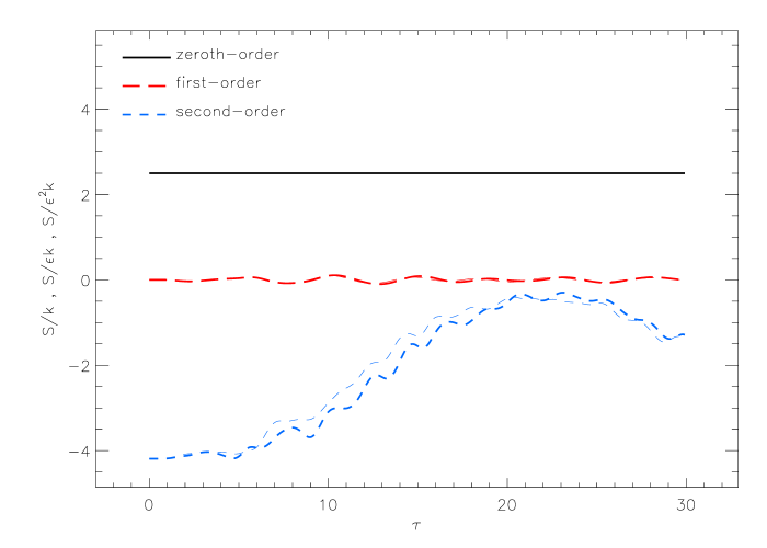
Figure 1: Evolution of the $(m,n)$ coarse-grained entropy contributions for an initial $c_{1,1}$ perturbation. To magnify the behaviors, each set of values has been divided by the corresponding perturbation strength. Thin lines illustrate test-particle values, while thick lines represent self-gravitating values. First-order entropy behaviors are marked with long dashed lines. Second-order entropy evolutions are marked with short dashed lines. The first-order curves remain nearly constant and show no differences between test-particle and self-gravitating systems. The second-order curves show noticeable increases, with the late-time decreases likely stemming from numerical issues. Differences between test-particle and self-gravitating systems are noticeable at this order, but the overall behaviors are rather similar.

Test-particle systems can only experience phase mixing, but perturbed self-gravitating systems have the possibility of experiencing violent relaxation in addition to phase mixing. In an attempt to disentangle the impact of each process on the entropy evolution, we compare coarse-grained entropy behaviors in test-particle and self-gravitating systems subject to identical perturbations. As shown in Figures 1 and 2, there do not appear to be significant or systematic differences between the behaviors in test-particle and self-gravitating situations. At least for the modest perturbation strengths investigated here, violent relaxation has a much smaller impact on entropy creation compared to phase mixing.

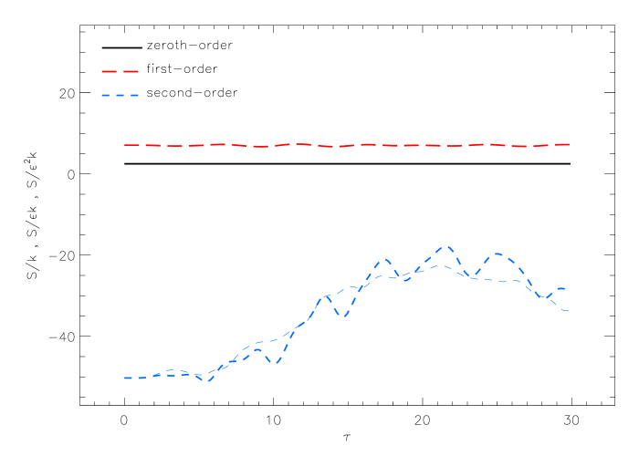
Figure 2: Evolution of the $(m,n)$ coarse-grained entropy contributions for an initial $c_{2,0}$ perturbation. As in Figure 1, the values for the various orders have been normalized by the appropriate perturbation strength. Again, the behaviors of the test-particle (thin) and self-gravitating (thick) curves are very similar at every order.

The behavior of the entropy is in line with the Tremaine et al. prediction that the coarse-grained entropy should not decrease from its initial value. The multiple, competing, terms present in Equation 61 are an expression of why a stronger statement cannot be made, like the guarantee of monotonic increase for collisional systems. The time-derivative of first-order entropy can be positive or negative, and while second-order entropy shows an overall increase during relaxation due to phase mixing, it is not a monotonic increase.

3.2.3 Non-linear Perturbation Simulations

Our perturbation analysis has led us to speculate that violent relaxation is not a significant source of entropy production. We have investigated whether or not this is simply an artifact of our limitations on perturbation strength. Using $N$-body simulations (for numerical method details see Barnes & Ragan, 2014), we have also explored entropy evolutions in self-gravitating and test-particle systems that are so far from equilibrium that our perturbation expressions are not appropriate. These initial conditions are “waterbags” (Joyce & Worrakitpoonpon, 2011) with different amounts of kinetic energy. For these $N$-body simulations, entropy is calculated using a particle counting scheme,

$$S_{\rm NB}=-\sum_{i}n_{i}\ln{n_{i}},$$ (62)

where $n$ is particle number and $i$ enumerates different areas of phase space (all of size $\Delta\chi\Delta\varpi$). Unlike in quantum situations where $\Delta\chi$ and $\Delta\varpi$ can be related to Planck’s constant, we have simply used trial and error to set sizes of the phase-space boxes. After investigating a wide range, we have found that values near the adopted $\Delta\chi=\Delta\varpi=2\times 10^{-2}$ produce entropy values that show the most obvious changes during evolution. Smaller values result in almost no particles falling into the boxes, while larger values produce boxes so large that variation is basically absent. In either case, resulting entropy changes are small.

Somewhat surprisingly, test-particle systems experience larger entropy changes during relaxation, as shown in Figure 3. We note that the maximum difference between test-particle and self-gravitating entropies is approximately 5% of either entropy value, again indicating that violent relaxation does not have a strong impact on entropy behavior. In agreement with the second-order results, differences between self-gravitating and test-particle systems disappear as the non-linearity of initial conditions decreases. Figure 4 shows how much smaller the entropy differences are when the system has half of the kinetic energy required for virial equilibrium and consequently undergoes a much milder relaxation.

Figure 3: Comparisons between ensemble average entropy behaviors in self-gravitating (panel a) and test-particle (panel b) $N$-body simulations starting from identical initial conditions. Particles are placed spatially according to a uniform distribution of random values. There is no initial kinetic energy, making this an extremely non-equilibrium distribution. That the test-particle entropy shows a larger change than in the self-gravitating case can be seen in panel c, where the self-gravitating entropy value minus the test-particle entropy value is shown as a function of time.

Figure 4: Analogous to Figure 3, but systems are given half of the virial equilibrium kinetic energy. This rectangular phase-space distribution is much closer to approximating equilibrium compared to the zero kinetic energy cases. Note that the overall changes to self-gravitating (panel a) and test-particle (panel b) entropies are greatly diminished compared to those in Figure 3. Again, panel c shows that the test-particle entropy shows a larger change than in the self-gravitating case.

3.2.4 Quantifying Incomplete Relaxation

Any perturbation involving only first-order coefficients leads to predictable time-independent modes (Ragan & Barnes, 2019). These time-independent sets of coefficient values lead to upper-limits on changes that coarse-grained entropy can experience. For example, any odd-$m$, odd-$n$ perturbation results in a time-independent mode where the only non-zero coefficient values exist at $m=n=\infty$. The loss of all of the structure information encoded in the coefficients results in a maximal gain in coarse-grained entropy. However, for perturbations that leave residual time-independent coefficients, the coarse-grained entropy value increases or decreases with the values of $M$ and $N$. Smaller coarse-graining boxes lead to smaller increases in entropy.

We have numerically determined time-independent modes, or sets of coefficients, and used them to calculate the maximum coarse-grained entropy change resulting from perturbations by individual $(m,n)$ coefficients. Behavior of odd-$m$, odd-$n$ perturbations has been described above, so we focus on even-$m$, even-$n$ perturbations. As the perturbing $m$ and $n$ values increase, the entropy change approaches the maximal value associated with complete relaxation. More physically, these curves show that perturbations with larger position and velocity scales (smaller $n$ and $m$ values) undergo substantially more incomplete relaxation.

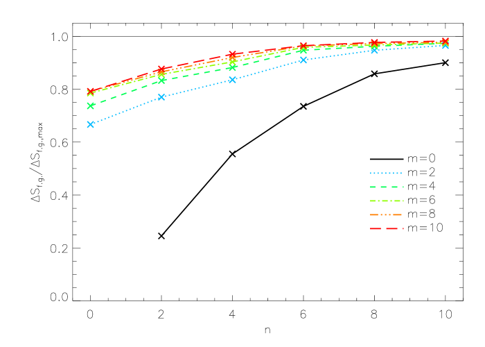
Figure 5: Differences in second-order fine-grained entropy between initial conditions and time-independent modes for several even-$m$, even-$n$ perturbations. As either $m$ or $n$ increase, the difference increases. A $(0,2)$ perturbation holds onto the maximum amount of its initial entropy during its evolution; it relaxes the smallest amount.

Qualitatively, the relationship between the entropy differences for $(m=2,n=0)$ and $(m=0,n=2)$ seen in Figure 5 agrees with the coarse-grained entropy changes seen in Figures 2 and 6. A $c_{0,2}$ perturbation is a significant contribution to a time-independent mode. As a result, there is relatively little relaxation that is possible.

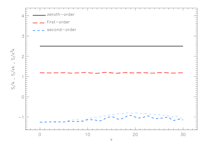
Figure 6: Evolution of the $(m,n)$ coarse-grained entropy contributions for an initial $c_{0,2}$ perturbation, with the same curve descriptions as in Figures 1 and 2. The entropy change present in this plot is noticeably smaller than those in Figures 1 and 2, indicating that the perturbation is more nearly a time-independent mode which can relax little.

As each time-independent mode corresponds to a unique amount of entropy, we think of the collection of these mode strengths as quantifying the amount of relaxation possible. If a given perturbation does not contain any time-independent modes, then a complete relaxation is possible. It is important to note that these kinds of perturbations also contain zero energy, so the system will return to its underlying separable equilibrium. Perturbations that are energetic must contain time-independent modes and preclude complete relaxation. As in Figures 2 and 6, the particular modes determine how incomplete the relaxation will be.

3.3 Thermodynamic Entropy

We have also taken a more standard thermodynamic approach to calculating the entropy in these models (de Groot & Mazur, 1985). To begin, we list relevant moments of the collisionless Boltzmann equation:

$$\mbox{zeroth moment,}\quad\frac{\partial}{\partial\tau}[\Lambda] = -\frac{\mathrm{d}}{\mathrm{d}\chi}\left[\Lambda\langle\varpi\rangle\right]$$

$$\mbox{first moment,}\quad\frac{\partial}{\partial\tau}[\Lambda\langle\varpi\rangle] = -\frac{\mathrm{d}}{\mathrm{d}\chi}\left[\Lambda\langle\varpi^{2}\rangle\right]-\Lambda\frac{\mathrm{d}\phi}{\mathrm{d}\chi}$$

$$\mbox{second moment,}\quad\frac{\partial}{\partial\tau}\left[\frac{\Lambda}{2}\langle\varpi^{2}\rangle\right] = -\frac{\mathrm{d}}{\mathrm{d}\chi}\left[\frac{\Lambda}{2}\langle\varpi^{3}\rangle\right]-\Lambda\langle\varpi\rangle\frac{\mathrm{d}\phi}{\mathrm{d}\chi}.$$

Our goal is to use the first law of thermodynamics,

$$\mathrm{d}u=T\mathrm{d}s-p\;\mathrm{d}L,$$ (63)

where $u$ is internal energy per unit mass, $T$ is temperature, $p$ is pressure, and $L$ is the extent of the system (the one-dimensional analogue to volume $V$), to understand how entropy changes. Keeping with typical definitions,

$$p\equiv\Lambda(\langle\varpi^{2}\rangle-\langle\varpi\rangle^{2}),$$ (64)

and

$$T\equiv\langle\varpi^{2}\rangle.$$ (65)

We use the angle brackets to denote average quantities that are calculated as

$$\langle A\rangle\equiv\frac{1}{\Lambda}\int_{-\infty}^{\infty}Af\;\mathrm{d}\varpi.$$ (66)

With these definitions, we find that

$$\Lambda\frac{\mathrm{d}}{\mathrm{d}\tau}\left[\frac{\langle\varpi^{2}\rangle-\langle\varpi\rangle^{2}}{2}\right]=-p\frac{\mathrm{d}\langle\varpi\rangle}{\mathrm{d}\chi}-$$ (67)

$$\frac{\mathrm{d}}{\mathrm{d}\chi}\left[\frac{\Lambda}{2}(\langle\varpi^{3}\rangle-3\langle\varpi^{2}\rangle\langle\varpi\rangle+2\langle\varpi\rangle^{3}\right].$$

Using the continuity equation (the zeroth moment from above), we can re-write the first term on the right-hand side of this expression as

$$\frac{\mathrm{d}\langle\varpi\rangle}{\mathrm{d}\chi}=\Lambda\frac{\mathrm{d}}{\mathrm{d}\tau}\left(\frac{1}{\Lambda}\right)=\Lambda\frac{\mathrm{d}L}{\mathrm{d}\tau}.$$ (68)

Identifying the internal energy per unit mass as,

$$u\equiv\frac{\langle\varpi^{2}\rangle-\langle\varpi\rangle^{2}}{2},$$ (69)

we can now re-cast Equation 67 as

$$\frac{\mathrm{d}u}{\mathrm{d}\tau}=-p\frac{\mathrm{d}L}{\mathrm{d}\tau}-\frac{1}{\Lambda}\frac{\mathrm{d}}{\mathrm{d}\chi}\left[\frac{\Lambda}{2}(\langle\varpi^{3}\rangle-3\langle\varpi^{2}\rangle\langle\varpi\rangle+2\langle\varpi\rangle^{3}\right].$$ (70)

This last term must be equal to $T\mathrm{d}s/\mathrm{d}\tau$, according to the first law of thermodynamics.

The entropy time-derivative can be manipulated further to cast it as two terms; one that represents a divergence of a flux and another that represents entropy creation. The result is that the entropy creation term takes the form,

$$\sigma\equiv\frac{\Lambda}{2\langle\varpi^{2}\rangle^{2}}(\langle\varpi^{3}\rangle-3\langle\varpi^{2}\rangle\langle\varpi\rangle+2\langle\varpi\rangle^{3})\frac{\mathrm{d}\langle\varpi^{2}\rangle}{\mathrm{d}\chi}.$$ (71)

For an equilibrium situation, the spatial derivative of $\langle\varpi^{2}\rangle$ is zero, guaranteeing that the state is an entropy maximum. Given this expression, the creation portion of the entropy time-derivative can be estimated by integrating Equation 71 over all space. The average velocity values required can be calculated straightforwardly from first- and second-order coefficient values. As shown in Figure 7, this thermodynamic calculation produces $\dot{S}$ values that are comparable to those determined from the coarse-grained values discussed above.

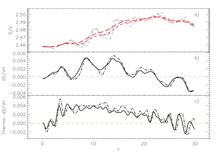
Figure 7: Panel a shows the evolution of the total $(m,n)$ coarse-grained entropy for an initial $c_{1,1}$ perturbation. The thin lines show the raw values, while the thick versions correspond to a smoothed set of values. Long- and short-dashed lines represent test-particle and self-gravitating systems, respectively. Panel b shows the time-derivative of the smoothed curves from panel a. The solid line corresponds to the test-particle evolution, while the dot-dashed line reflects the changes in the self-gravitating behavior. Panel c contains the thermodynamic estimate of $\dot{S}$ based on Equation 71. The line styles in this panel are the same as in panel b.

4 Energy Distributions

Entropy evolution is only marginally affected by violent relaxation. Time-independent mode strengths provide a way to quantify the incompleteness of a relaxation, and those modes are different between test-particle and self-gravitating systems. In this section, we discuss how energy distributions $n(\beta E)$, the number of particles with a given energy, can isolate the impact of violent relaxation. Test particle systems cannot show any $n(\beta E)$ evolution as their potentials are fixed. On the other hand, the potential oscillations that accompany violent relaxation allow mass to change its energy. The total change to $n(\beta E)$ can be broken into contributions from different $c_{m,n}$ as follows.

For a first-order perturbation like that in Equation 13, we define an energy-distribution perturbation through,

$$\int\int f_{mn,1}\,\mathrm{d}\chi\mathrm{d}\varpi=\int n_{mn,1}\,\mathrm{d}(\beta E),$$ (72)

where the integrals run over all possible values. As usual, we understand $n_{mn,1}$ by re-writing the left-hand side of this equation in terms of an energy integral so that the integrands can be equated. With the decomposition in Equation 14, this leads to

$$n_{mn,1}(\beta E)=c_{m,n}e^{-\beta E}\int_{q1}^{q2}\frac{H_{m}\left[\sqrt{\beta E-\beta\Phi(q)}\right]P_{n}(q)e^{\beta\Phi(q)}}{\sqrt{\beta E-\beta\Phi(q)}}\,\mathrm{d}q.$$ (73)

Here, $q=\tanh{\chi}$, $q1=\tanh{\chi_{\rm max}}$, $q2=-\tanh{\chi_{\rm max}}$, and $\chi_{\rm max}$ is the turning point location found by solving $\beta E=\beta\Phi(\chi_{\rm max})$. Equation 73 gives us the change from an equilibrium $n(\beta E)$ that arises from any given $(m,n)$ coefficient. As an example, Figure 8 shows the change in the energy distribution due to a first-order $m=1$, $n=2$ perturbation. This perturbation was chosen because it is non-energetic and allows for substantial simplification in Equation 73. For $m=1$ perturbations, the Hermite term and the radical in the denominator of Equation 73 cancel. With this, it is straightforward to show that a perturbation like $m=1$, $n=1$ will lead to no change in $n(\beta E)$. Changes to $n(\beta E)$ due to energetic perturbations are more involved, but their overall behavior is similar to that shown in Figure 8. Depending on the sign of the perturbing coefficient, particles can be shifted towards lower or higher energies. These types of calculations coupled with coefficient evolutions can be used to determine how the complete energy distribution perturbation,

$$n_{1}(\beta E)=\sum_{m,n}n_{mn,1}(\beta E),$$ (74)

evolves.

Figure 8: Based on Equation 73, the impact of a single perturbing coefficient on the energy distribution can be calculated. Shown here is the shape of the change induced by a first-order $c_{1,2}$ perturbation. Note that depending on the sign of the perturbing coefficient, the loss/gain in particles can be made to occur for either higher or lower energies.

From self-gravitating $N$-body simulations, we can verify these relationships by approximating $n(\beta E)$ distributions with histograms of the numbers of particles in finite width energy bins. For an initial $c_{1,1}$ perturbation, Figure 9 illustrates that 1) the distribution is initially the same as the separable equilibrium (as expected based on Equation 73) and 2) there is no net change to the energy distribution once the system has reached a steady-state. It is important to realize that $n(\beta E)$ changes during the evolution, but eventually settles back to equilibrium. Any (odd-$m$, odd-$n$) perturbation will behave similarly.

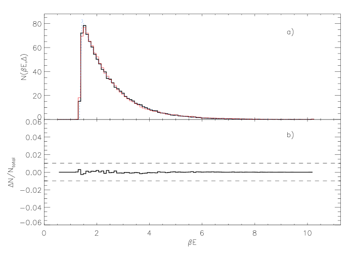
Figure 9: Approximating changes to $n(\beta E)$ using histograms of particle numbers in an $N$-body simulation of a system with an initial $c_{1,1}$ perturbation. Panel a shows an initial state histogram (thick line), a final steady-state histogram (thin line), and a curve showing how a separable equilibrium histogram would behave (thin dotted line) given the same bin widths. Panel b shows the difference between the two histograms (solid line) along with average error-in-the-mean values determined from the ensembles (dashed lines).

For contrast, Figures 10 and 11 show how the energetic perturbations $c_{0,2}$ and $c_{2,0}$ alter the energy distribution and lead to permanent distribution changes, respectively. We argue that these changes are real as the shift in the peak shape seen involves changes that are larger than, or at least comparable to, statistical uncertainties in bin occupations. At no point do the distributions follow the equilibrium behavior.

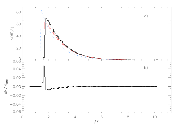
Figure 10: Approximating changes to $n(\beta E)$ using histograms of particle numbers in an $N$-body simulation of a system with an initial $c_{0,2}$ perturbation. The panels and line styles are the same as those in Figure 9. We argue that the shift in the distribution shape is real as the differences are bigger than or comparable to the statistical fluctuations.

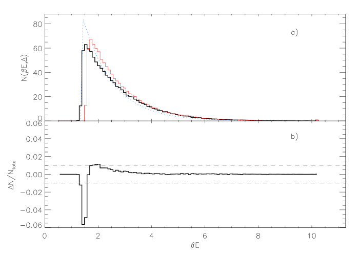
Figure 11: Approximating changes to $n(\beta E)$ using histograms of particle numbers in an $N$-body simulation of a system with an initial $c_{2,0}$ perturbation. The panels and line styles are the same as those in Figure 9.

The $n(\beta E)$ distribution for a $c_{1,1}$ perturbation oscillates between deviations like those in Figures 10 and 11 at various points in its early evolution, before reaching a steady-state. These changes to $n(\beta E)$ are easy to visually inspect, but we want to quantify the impact of violent relaxation. To do so, we use the common chi-squared test for differences between binned distributions (Press et al., 1994). We calculate the $\chi^{2}$ value between the initial and subsequent distributions as a function of time. At each output time, the difference between the distributions is squared and then normalized by the sum of the distributions’ values in each bin.

Integrating $\chi^{2}(t)$ over the evolution gives us a measure of the impact of violent relaxation. For a test-particle system, there is never any change to $n(\beta E)$, $\chi^{2}(t)=0$, and integrating over time gives zero. For self-gravitating perturbations, $\chi^{2}$ asymptotes to a constant value. A $c_{1,1}$ perturbation has $\chi^{2}(t=\infty)=0$, as it returns to equilibrium. However, $c_{0,2}$ and $c_{2,0}$ perturbations have non-zero values of $\chi^{2}(t=\infty)$. We calculate the violent relaxation measure as,

$$\mathcal{V}=\int_{0}^{\infty}[\chi^{2}(t)-\chi^{2}(\infty)]\;\mathrm{d}t.$$ (75)

$\mathcal{V}$ values are negative if $\chi^{2}(t)$ tends to be lower than $\chi^{2}(\infty)$ during relaxation. In the systems investigated here, $\chi^{2}(t)$ is an oscillating function. A negative $\mathcal{V}$ value indicates that a system spends more time closer to its original energy distribution when compared to a system with a positive $\mathcal{V}$ value. For perturbations like the ones shown in Figures 9, 10, and 11, the $c_{0,2}$ case produces a negative $\mathcal{V}$ value. With the same perturbation strength, $c_{1,1}$ perturbations produce $|\mathcal{V}|$ values that are many times larger than those resulting from $c_{0,2}$ and $c_{2,0}$ perturbations.

Given that a system with a $c_{0,2}$ perturbation is closer to a time-independent state than one with a $c_{2,0}$ perturbation, which is still closer than one with a $c_{1,1}$ perturbation, we suggest the following interpretation of self-gravitating $\mathcal{V}$ values. Negative values reflect a system that undergoes relatively little relaxation. The most positive values, for a given perturbation strength, indicate that systems will return to their original separable equilibrium after undergoing substantial relaxation.

5 Summary

Collisionless one-dimensional gravitating systems are taken as testbeds for analyzing relaxation processes. Unlike three-dimensional situations, the one-dimensional models investigated here possess separable-solution equilibria with Boltzmann form that we perturb. Using second-order perturbation theory, we investigate relaxation of these systems in terms of entropy production. Coefficient dynamics simulations allow us to track fine- and coarse-grained entropy behavior as perturbed systems settle to steady states.

We have presented two specific routes for calculating coarse-grained entropy. One is based on the more traditional “binning” of phase space which looks at how a distribution function changes over finite-sized regions of phase space, $\Delta\chi\Delta\varpi$. The more appealing definition coarse-grains in a coefficient space formed by decomposing distributions as series of Hermite-Legendre function products. Ignoring small-scale structure by including only low-order coefficients (small $m$ and $n$ values) provides us with a simple conceptual picture, when combined with coefficient dynamics. General perturbations have time-dependent and time-independent components. Time-dependent perturbations involve oscillating coefficients that decay as a wave-like pattern expands to larger $m$ and $n$ values. These waves represent phase mixing and as the coefficients inside a coarse-graining box decrease, the entropy increases. On the other hand, any time-independent component that is present leaves an imprint on the coarse-grained entropy. These time-independent modes essentially limit the entropy that can be gained by the system. Their presence guarantees that the separable equilibrium cannot be reached through either phase mixing or violent relaxation routes.

In the terminology of (Tremaine et al.1986), using Maxwell-Boltzmann (or Lynden-Bell) entropy as an H-function demonstrates that their collisionless analogue to the H-theorem holds. Unlike the entropy behavior determined by the collisional H-theorem, relaxation in these systems cannot be guaranteed to monotonically increase entropy. However, terms strongly impacted by phase mixing dominate overall changes in entropy, leading to increases.

One point of interest is that phase mixing appears to have a much larger impact on entropy than does violent relaxation. Our initial expectation was that self-gravitating systems should show faster and/or larger entropy changes as a result of the additional relaxation mechanism. However, test-particle simulations show roughly the same increases over the same time-scales as those corresponding to self-gravitating systems. The impact of violent relaxation can be quantified according to how a system’s energy distribution changes during an evolution.

Appendix A Test-particle Coefficient Dynamics

This appendix demonstrates that

$$\frac{\partial}{\partial\tau}\sum_{m,n\geq 0}\frac{2^{m}m!}{2n+1}\left[c_{m,n}^{\rm test}\right]^{2}=0.$$ (76)

To do this we will use the test-particle coefficient dynamics equations that link diagonal nearest-neighbor values to time-derivatives in the following way,

$$\dot{c}_{j,k}^{\rm test}=\frac{k(k-1)}{2(2n-1)}c_{j-1,k-1}^{\rm test}-\frac{(k+1)(k+2)}{2(2n+3)}c_{j-1,k+1}^{\rm test}+$$ (77)

$$\frac{(j+1)k(k+1)}{2n-1}c_{j+1,k-1}^{\rm test}-\frac{(j+1)k(k+1)}{2n+3}c_{j+1,k+1}^{\rm test}.$$

For concreteness, we isolate two nearest-neighbor points, $(j,k)$ and $(j+1,k+1)$. Expanding the $(m=j,n=k)$ term in Equation 76 using the coefficient dynamics equations leads to a link to the $(j+1,k+1)$ coefficient,

$$\frac{-2^{j+1}(j+1)!k(k+1)}{(2n+1)(2n+3)}c_{j,k}^{\rm test}c_{j+1,k+1}^{\rm test}.$$ (78)

Writing the $(m=j+1,n=k+1)$ term in Equation 76 and using the coefficient dynamics equations produces a link to the $(j,k)$ coefficient,

$$\frac{2^{j+1}(j+1)!k(k+1)}{(2n+1)(2n+3)}c_{j,k}^{\rm test}c_{j+1,k+1}^{\rm test}.$$ (79)

Similar arguments can be made for the $(m=j-1,n=k+1)$, $(m=j-1,n=k-1)$, and $(m=j+1,n=k-1)$ terms. The quantity being summed in Equation 76 is transferred between terms, but is not created or destroyed. Summing over all possible values of $m$ and $n$ guarantees that Equation 76 is true.

Appendix B Second-order $(x,v)$ Coarse-grained Entropy

As with the first-order coarse-grained entropy expressions (Equations 3.2.1 and 55), the $(x,v)$ coarse-graining produces a second-order entropy expression that is much more complicated than the analogous $(m,n)$ coarse-graining version. From Equation 52, the coarse-graining corrections to the second order entropy are,

$$\iint\gamma_{xv,2}(1+\ln{f_{0}})\,\mathrm{d}\chi\mathrm{d}\varpi+$$ (80)

$$\frac{1}{2}\iint\frac{\gamma_{xv,1}^{2}}{f_{0}}\,\mathrm{d}\chi\mathrm{d}\varpi+\iint\frac{\gamma_{xv,1}f_{1}}{f_{0}}\,\mathrm{d}\chi\mathrm{d}\varpi.$$

The first term is analogous to the first-order correction term (Equation 3.2.1), with $c_{0,n}$ replaced by $d_{0,n}$. Since $\gamma_{xv}$ terms involve the small quantity $\Delta^{2}$, the second term should be much smaller than the first and third, and we ignore it here. Finally, the third term can be shown to be,

$$\iint\frac{\gamma_{xv,1}f_{1}}{f_{0}}\,\mathrm{d}\chi\mathrm{d}\varpi=$$ (81)

$$\pi\frac{\Delta^{2}}{6}\sum_{m,n\atop m\neq n=0}\left[\frac{2^{m+2}(m+2)!}{2n+1}c_{m+2,n}c_{m,n}+\right.$$

$$\frac{2^{m}m!}{2n+5}(A_{n}+C_{n}Q_{0}^{(2,n)})c_{m,n+2}c_{m,n}+$$

$$\frac{2^{m}m!}{2n+1}(B_{n}+C_{n}Q_{2}^{(2,n)})c_{m,n}^{2}+$$

$$\left.\frac{2^{m}m!}{2n-3}C_{n}Q_{4}^{(2,n)}c_{m,n-2}c_{m,n}\right].$$

The complexity of the terms in this expression makes a simple interpretation of the coarse-grained entropy time-behavior difficult. However, numerically following the coefficient behavior allows us to calculate this quantity during an evolution. The results are shown in Figure 12.

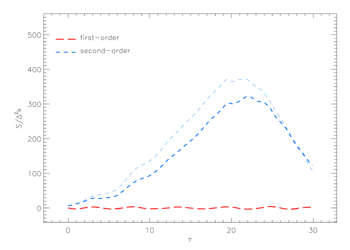
Figure 12: Evolution of the $(x,v)$ coarse-grained entropy for a system with an initial $c_{1,1}$ perturbation. Thin lines show the behavior for a test particle case, thick lines correspond to the self-gravitating case. As with the $(m,n)$ coarse-graining, first-order coarse-grained entropy is essentially constant. Changes are appreciable at second-order only.

References

- Barnes & Ragan (2014) Barnes E.I., Ragan R.J., 2014, MNRAS, 437, 2340
- Barnes & Williams (2012) Barnes E.I., Williams L.L.R., 2012, ApJ, 748, 144
- Binney & Tremaine (1987) Binney J., Tremaine S., 1987, Galactic Dynamics. Princeton Univ. Press, Princeton, NJ
- Camm (1950) Camm G.L., 1950, MNRAS, 110, 305
- de Groot & Mazur (1985) de Groot S., Mazur X., 1985, Non-equilibrium Thermodynamics. Dover, New York, NY
- Dougall (1953) Dougall J., 1953, Glasgow Mathematical Journal, 1, 121
- Hjorth & Williams (2010) Hjorth J., Williams L.L.R., 2010, ApJ, 722, 851
- Joyce & Worrakitpoonpon (2010) Joyce M., Worrakitpoonpon T., 2010, J. Stat. Mech. Theory & Experiment, 10, 12
- Joyce & Worrakitpoonpon (2011) Joyce M., Worrakitpoonpon T., 2011, Phys. Rev. E, 84, 1139
- Levin et al. (2014) Levin Y., Pakter R., Rizzato F.B., Teles T.N., Benetti F.P.C., 2014, Physics Reports, 535, 1
- Lynden-Bell (1967) Lynden-Bell D., 1967, MNRAS, 136, 101
- Press et al. (1994) Press W.H., Teukolsky S.A., Vetterling W.T., Flannery B.P. 1994, Numerical Recipes. Cambridge University Press, New York, NY
- Ragan & Barnes (2019) Ragan R.J., Barnes E.I., 2019, MNRAS, submitted
- Rybicki (1971) Rybicki G.B., 1971, Ap&SS, 14, 56
- (15) Tremaine S., Hénon M., Lynden-Bell D. 1986, MNRAS, 219, 285