GENO – GENeric Optimization
for Classical Machine Learning

Abstract

Although optimization is the longstanding algorithmic backbone of machine learning, new models still require the time-consuming implementation of new solvers. As a result, there are thousands of implementations of optimization algorithms for machine learning problems. A natural question is, if it is always necessary to implement a new solver, or if there is one algorithm that is sufficient for most models. Common belief suggests that such a one-algorithm-fits-all approach cannot work, because this algorithm cannot exploit model specific structure and thus cannot be efficient and robust on a wide variety of problems. Here, we challenge this common belief. We have designed and implemented the optimization framework GENO (GENeric Optimization) that combines a modeling language with a generic solver. GENO generates a solver from the declarative specification of an optimization problem class. The framework is flexible enough to encompass most of the classical machine learning problems. We show on a wide variety of classical but also some recently suggested problems that the automatically generated solvers are (1) as efficient as well-engineered specialized solvers, (2) more efficient by a decent margin than recent state-of-the-art solvers, and (3) orders of magnitude more efficient than classical modeling language plus solver approaches.

1 Introduction

Optimization is at the core of machine learning and many other fields of applied research, for instance operations research, optimal control, and deep learning. The latter fields have embraced frameworks that combine a modeling language with only a few optimization solvers; interior point solvers in operations research and stochastic gradient descent (SGD) and variants thereof in deep learning frameworks like TensorFlow, PyTorch, or Caffe. That is in stark contrast to classical (i.e., non-deep) machine learning, where new problems are often accompanied by new optimization algorithms and their implementation. However, designing and implementing optimization algorithms is still a time-consuming and error-prone task.

The lack of an optimization framework for classical machine learning problems can be explained partially by the common belief, that any efficient solver needs to exploit problem specific structure. Here, we challenge this common belief.

We introduce GENO (GENeric Optimization), an optimization framework that allows to state optimization problems in an easy-to-read modeling language. From the specification an optimizer is automatically generated by using automatic differentiation on a symbolic level. The optimizer combines a quasi-Newton solver with an augmented Lagrangian approach for handling constraints.

Any generic modeling language plus solver approach frees the user from tedious implementation aspects and allows to focus on modeling aspects of the problem at hand. However, it is required that the solver is efficient and accurate. Contrary to common belief, we show here that the solvers generated by GENO are (1) as efficient as well-engineered, specialized solvers at the same or better accuracy, (2) more efficient by a decent margin than recent state-of-the-art solvers, and (3) orders of magnitude more efficient than classical modeling language plus solver approaches.

Related work.

Classical machine learning is typically served by toolboxes like scikit-learn [62], Weka [32], and MLlib [53]. These toolboxes mainly serve as wrappers for a collection of well-engineered implementations of standard solvers like LIBSVM [14] for support vector machines or glmnet [33] for generalized linear models. A disadvantage of the toolbox approach is a lacking of flexibility. An only slightly changed model, for instance by adding a non-negativity constraint, might already be missing in the framework.

Modeling languages provide more flexibility since they allow to specify problems from large problem classes. Popular modeling languages for optimization are CVX [21, 38] for MATLAB and its Python extension CVXPY [3, 24], and JuMP [28] which is bound to Julia. In the operations research community AMPL [31] and GAMS [10] have been used for many years. All these languages take an instance of an optimization problem and transform it into some standard form of a linear program (LP), quadratic program (QP), second-order cone program (SOCP), or semi-definite program (SDP). The transformed problems is then addressed by solvers for the corresponding standard form. However, the transformation into standard form can be inefficient, because the formal representation in standard form can grow substantially with the problem size. This representational inefficiency directly translates into computational inefficiency.

The modeling language plus solver paradigm has been made deployable in the CVXGEN [52], QPgen [35], and OSQP [4] projects. In these projects code is generated for the specified problem class. However, the problem dimension and sometimes the underlying sparsity pattern of the data needs to be fixed. Thus, the size of the generated code still grows with a growing problem dimension. All these projects are targeted at embedded systems and are optimized for small or sparse problems. The underlying solvers are based on Newton-type methods that solve a Newton system of equations by direct methods. Solving these systems is efficient only for small problems or problems where the sparsity structure of the Hessian can be exploited in the Cholesky factorization. Neither condition is typically met in standard machine learning problems.

Deep learning frameworks like TensorFlow [1], PyTorch [61], or Caffe [43] are efficient and fairly flexible. However, they target only deep learning problems that are typically unconstrained problems that ask to optimize a separable sum of loss functions. Algorithmically, deep learning frameworks usually employ some form of stochastic gradient descent (SGD) [66], the rationale being that computing the full gradient is too slow and actually not necessary. A drawback of SGD-type algorithms is that they need careful parameter tuning of, for instance, the learning rate or, for accelerated SGD, the momentum. Parameter tuning is a time-consuming and often data-dependent task. A non-careful choice of these parameters can turn the algorithm slow or even cause it to diverge. Also, SGD type algorithms cannot handle constraints.

GENO, the framework that we present here, differs from the standard modeling language plus solver approach by a much tighter coupling of the language and the solver. GENO does not transform problem instances but whole problem classes, including constrained problems, into a very general standard form. Since the standard form is independent of any specific problem instance it does not grow for larger instances. GENO does not require the user to tune parameters and the generated code is highly efficient.

Table 1: Comparison of approaches/frameworks for optimization in machine learning.

	handwritten	TensorFlow,	Weka,	CVXPY	GENO
	solver	PyTorch	Scikit-learn
flexible	✗	✓	✗	✓	✓
efficient	✓	✓	✓	✗	✓
deployable / stand-alone	✓	✗	✗	✗	✓
can accommodate constraints	✓	✗	✓	✓	✓
parameter free (learning rate, …)	✗/✓	✗	✓	✓	✓
allows non-convex problems	✓	✓	✓	✗	✓

2 The GENO Pipeline

GENO features a modeling language and a solver that are tightly coupled. The modeling language allows to specify a whole class of optimization problems in terms of an objective function and constraints that are given as vectorized linear algebra expressions. Neither the objective function nor the constraints need to be differentiable. Non-differentiable problems are transformed into constrained, differentiable problems. A general purpose solver for constrained, differentiable problems is then instantiated with the objective function, the constraint functions and their respective gradients. The gradients are computed by the matrix calculus algorithm that has been recently published in [47]. The tight integration of the modeling language and the solver is possible only because of this recent progress in computing derivatives of vectorized linear algebra expressions.

Generating a solver takes only a few milliseconds. Once it has been generated the solver can be used like any hand-written solver for every instance of the specified problem class. An online interface to the GENO framework can be found at http://www.geno-project.org.

2.1 Modeling Language

A GENO specification has four blocks (cf. the example to the right that shows an $\ell_{1}$-norm minimization problem from compressed sensing where the signal is known to be an element from the unit simplex.): (1) Declaration of the problem parameters that can be of type Matrix, Vector, or Scalar, (2) declaration of the optimization variables that also can be of type Matrix, Vector, or Scalar, (3) specification of the objective function in a MATLAB-like syntax, and finally (4) specification of the constraints, also in a MATLAB-like syntax that supports the following operators and functions: +, -, *, /, .*, ./, $\wedge$, $.\wedge$, log, exp, sin, cos, tanh, abs, norm1, norm2, sum, tr, det, inv. The set of operators and functions can be expanded when needed.

 

   

  parameters 

       Matrix A 

       Vector b 

  variables 

       Vector x 

  min 

       norm1(x) 

  st 

       A*x == b 

       sum(x) == 1 

       x >= 0 

   

 

Note that in contrast to instance-based modeling languages like CVXPY no dimensions have to be specified. Also, the specified problems do not need to be convex. In the non-convex case, only a local optimal solution will be computed.

2.2 Generic Optimizer

At its core, GENO’s generic optimizer is a solver for unconstrained, smooth optimization problems. This solver is then extended to handle also non-smooth and constrained problems. In the following we first describe the smooth, unconstrained solver before we detail how it is extended to handling non-smooth and constrained optimization problems.

Solver for unconstrained, smooth problems.

There exist quite a number of algorithms for unconstrained optimization. Since in our approach we target problems with a few dozen up to a few million variables, we decided to build on a first-order method. This still leaves many options. Nesterov’s method [58] has an optimal theoretical running time, that is, its asymptotic running time matches the lower bounds in $\Omega(1/\sqrt{\varepsilon})$ in the smooth, convex case and $\Omega(\log(1/\varepsilon))$ in the strongly convex case with optimal dependence on the Lipschitz constants $L$ and $\mu$ that have to be known in advance. Here $L$ and $\mu$ are upper and lower bounds, respectively, on the eigenvalues of the Hessian. On quadratic problems quasi-Newton methods share the same optimal convergence guarantee [42, 57] without requiring the values for these parameters. In practice, quasi-Newton methods often outperform Nesterov’s method, although they cannot beat it in the worst case. It is important to keep in mind that theoretical running time guarantees do not always translate into good performance in practice. For instance, even the simple subgradient method has been shown to have a convergence guarantee in $O(\log(1/\varepsilon))$ on strongly convex problems [37], but it is certainly not competitive on real world problems.

Hence, we settled on a quasi-Newton method and implemented the well-established L-BFGS-B algorithm [11, 73] that can also handle box constraints on the variables. It serves as the solver for unconstrained, smooth problems. The algorithm combines the standard limited memory quasi-Newton method with a projected gradient path approach. In each iteration, the gradient path is projected onto the box constraints and the quadratic function based on the second-order approximation (L-BFGS) of the Hessian is minimized along this path. All variables that are at their boundaries are fixed and only the remaining free variables are optimized using the second-order approximation. Any solution that is not within the bound constraints is projected back onto the feasible set by a simple min/max operation [54]. Only in rare cases, a projected point does not form a descent direction. In this case, instead of using the projected point, one picks the best point that is still feasible along the ray towards the solution of the quadratic approximation. Then, a line search is performed for satisfying the strong Wolfe conditions [71, 72]. This condition is necessary for ensuring convergence also in the non-convex case. The line search also obliterates the need for a step length or learning rate that is usually necessary in SGD, subgradient algorithms, or Nesterov’s method. Here, we use the line search proposed in [55] which we enhanced by a simple backtracking line search in case the solver enters a region where the function is not defined.

Solver for unconstrained non-smooth problems.

Machine learning often entails non-smooth optimization problems, for instance all problems that employ $\ell_{1}$-regularization. Proximal gradient methods are a general technique for addressing such problems [63]. Here, we pursue a different approach. All non-smooth convex optimization problems that are allowed by our modeling language can be written as $\min_{x}\{\max_{i}f_{i}(x)\}$ with smooth functions $f_{i}(x)$ [59]. This class is flexible enough to accommodate most of the non-smooth objective functions encountered in machine learning. All problems in this class can be transformed into constrained, smooth problems of the form

$$\begin{array}[]{rl}\displaystyle\min_{t,x}&t\\ \operatorname{s.t.}&f_{i}(x)\leq t.\end{array}$$

The transformed problems can then be solved by the solver for constrained, smooth optimization problems that we describe next.

Solver for smooth constrained problems.

There also quite a few options for solving smooth, constrained problems, among them projected gradient methods, the alternating direction method of multipliers (ADMM) [9, 34, 36], and the augmented Lagrangian approach [40, 64]. For GENO, we decided to follow the augmented Lagrangian approach, because this allows us to (re-)use our solver for smooth, unconstrained problems directly. Also, the augmented Lagrangian approach is more generic than ADMM. All ADMM-type methods need a proximal operator that cannot be derived automatically from the problem specification and a closed-form solution is sometimes not easy to compute. Typically, one uses standard duality theory for deriving the prox-operator. In [63], prox-operators are tabulated for several functions.

The augmented Lagrangian method can be used for solving the following general standard form of an abstract constrained optimization problem

$$\begin{array}[]{rl}\displaystyle\min_{x}&f(x)\\ \operatorname{s.t.}&h(x)=0\\ &g(x)\leq 0,\end{array}$$ (1)

where $x\in\mathbb{R}^{n}$, $f\colon\mathbb{R}^{n}\to\mathbb{R}$, $h\colon\mathbb{R}^{n}\to\mathbb{R}^{m}$, $g\colon\mathbb{R}^{n}\to\mathbb{R}^{p}$ are differentiable functions, and the equality and inequality constraints are understood component-wise.

The augmented Lagrangian of Problem (1) is the following function

$$L_{\rho}(x,\lambda,\mu)=f(x)+\frac{\rho}{2}\left\|h(x)+\frac{\lambda}{\rho}\right\|^{2}+\frac{\rho}{2}\left\|\left(g(x)+\frac{\mu}{\rho}\right)_{+}\right\|^{2},$$

where $\lambda\in\mathbb{R}^{m}$ and $\mu\in\mathbb{R}_{\geq 0}^{p}$ are Lagrange multipliers, $\rho>0$ is a constant, $\left\|\cdot\right\|$ denotes the Euclidean norm, and $(v)_{+}$ denotes $\max\{v,0\}$. The Lagrange multipliers are also referred to as dual variables. In principle, the augmented Lagrangian is the standard Lagrangian of Problem (1) augmented with a quadratic penalty term. This term provides increased stability during the optimization process which can be seen for example in the case that Problem (1) is a linear program. Note, that whenever Problem (1) is convex, i.e., $h$ are affine functions and $g$ are convex in each component, then the augmented Lagrangian is also a convex function.

The Augmented Lagrangian Algorithm 1 runs in iterations. In each iteration it solves an unconstrained smooth optimization problem. Upon convergence, it will return an approximate solution $x$ to the original problem along with an approximate solution of the Lagrange multipliers for the dual problem. If Problem (1) is convex, then the algorithm returns the global optimal solution. Otherwise, it returns a local optimum [5]. The update of the multiplier $\rho$ can be ignored and the algorithm still converges [5]. However, in practice it is beneficial to increase it depending on the progress in satisfying the constraints [6]. If the infinity norm of the constraint violation decreases by a factor less than $\tau=1/2$ in one iteration, then $\rho$ is multiplied by a factor of two.

Algorithm 1 Augmented Lagrangian Algorithm

1:  input: instance of Problem 1

2:  output: approximate solution $x\in\mathbb{R}^{n},\lambda\in\mathbb{R}^{p},\mu\in\mathbb{R}_{\geq 0}^{m}$

3:  initialize $x^{0}=0$, $\lambda^{0}=0$, $\mu^{0}=0$, and $\rho=1$

4:  repeat

5:     $x^{k+1}:=\quad\operatorname{argmin}_{x}\,L_{\rho}(x,\lambda^{k},\mu^{k})$

6:     $\lambda^{k+1}:=\quad\lambda^{k}+\rho h(x^{k+1})$

7:     $\mu^{k+1}:=\quad\left(\mu^{k}+\rho g(x^{k+1})\right)_{+}$

8:     update $\rho$

9:  until convergence

10:  return  $x^{k},\lambda^{k},\mu^{k}$

3 Limitations

While GENO is very general and efficient, as we will demonstrate in the experimental Section 4, it also has some limitations that we discuss here. For small problems, i.e., problems with only a few dozen variables, Newton-type methods with a direct solver for the Newton system can be even faster. GENO also does not target deep learning applications, where gradients do not need to be computed fully but can be sampled.

Some problems can pose numerical problems, for instance problems containing an $\exp$ operator might cause an overflow/underflow. However, this is a problem that is faced by all frameworks. It is usually addressed by introducing special operators like logsumexp.

Furthermore, GENO does not perform sanity checks on the provided input. Any syntactically correct problem specification is accepted by GENO as a valid input. For example, $\log(\det(xx^{\top}))$, where $x$ is a vector, is a valid expression. But the determinant of the outer product will always be zero and hence, taking the logarithm will fail. It lies within the responsibility of the user to make sure that expressions are mathematically valid.

4 Experiments

We conducted a number of experiments to show the wide applicability and efficiency of our approach. For the experiments we have chosen classical problems that come with established well-engineered solvers like logistic regression or elastic net regression, but also problems and algorithms that have been published at NeurIPS and ICML only within the last few years. The experiments cover smooth unconstrained problems as well as constrained, and non-smooth problems. To prevent a bias towards GENO, we always used the original code for the competing methods and followed the experimental setup in the papers where these methods have been introduced. We ran the experiments on standard data sets from the LIBSVM data set repository, and, in some cases, on synthetic data sets on which competing methods had been evaluated in the corresponding papers.

Specifically, our experiments cover the following problems and solvers: $\ell_{1}$- and $\ell_{2}$-regularized logistic regression, support vector machines, elastic net regression, non-negative least squares, symmetric non-negative matrix factorization, problems from non-convex optimization, and compressed sensing. Among other algorithms, we compared against a trust-region Newton method with conjugate gradient descent for solving the Newton system, sequential minimal optimization (SMO), dual coordinate descent, proximal methods including ADMM and variants thereof, interior point methods, accelerated and variance reduced variants of SGD, and Nesterov’s optimal gradient descent. Please refer to the appendix for more details on the solvers and GENO models.

Our test machine was equipped with an eight-core Intel Xeon CPU E5-2643 and 256GB RAM. As software environment we used Python 3.6, along with NumPy 1.16, SciPy 1.2, and scikit-learn 0.20. In some cases the original code of competing methods was written and run in MATLAB R2019. The solvers generated by GENO spent between $80\%$ and $99\%$ of their time on evaluating function values and gradients. Here, these evaluations essentially reduce to evaluating linear algebra expressions. Since all libraries are linked against the Intel MKL, running times of the GENO solvers are essentially the same in both environments, Python and MATLAB, respectively.

4.1 Regularization Path for $\ell_{1}$-regularized Logistic Regression

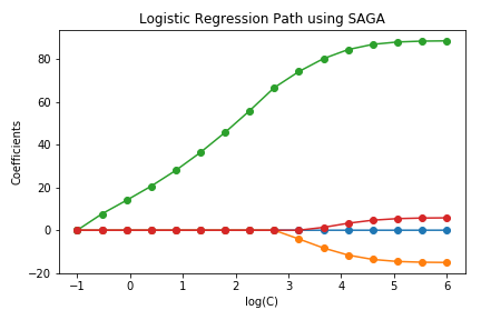
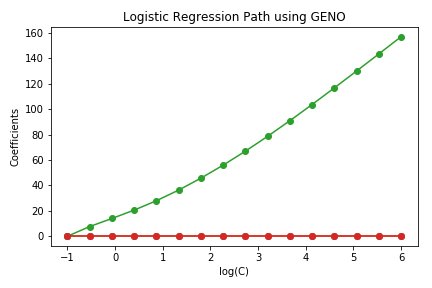
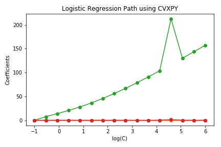
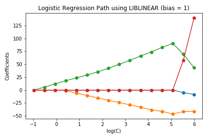
Figure 1: The regularization path of $\ell_{1}$-regularized logistic regression for the Iris data set using SAGA, GENO, CVXPY, and LIBLINEAR.

Computing the regularization path of the $\ell_{1}$-regularized logistic regression problem [20] is a classical machine learning problem, and only boring at a first glance. The problem is well suited for demonstrating the importance of both aspects of our approach, namely flexibility and efficiency. As a standard problem it is covered in scikit-learn. The scikit-learn implementation features the SAGA algorithm [23] for computing the whole regularization path that is shown in Figure 1. This figure can also be found on the scikit-learn website . However, when using GENO, the regularization path looks different, see also Figure 1. Checking the objective functions values reveals that the precision of the SAGA algorithm is not enough for tracking the path faithfully. GENO’s result can be reproduced by using CVXPY except for one outlier at which CVXPY did not compute the optimal solution. LIBLINEAR [30, 75] can also be used for computing the regularization path, but also fails to follow the exact path. This can be explained as follows: LIBLINEAR also does not compute optimal solutions, but more importantly, in contrast to the original formulation, it penalizes the bias for algorithmic reasons. Thus, changing the problem slightly can lead to fairly different results.

CVXPY, like GENO, is flexible and precise enough to accommodate the original problem formulation and to closely track the regularization path. But it is not as efficient as GENO. On the problem used in Figure 1 SAGA takes 4.3 seconds, the GENO solver takes 0.5 seconds, CVXPY takes 13.5 seconds, and LIBLINEAR takes 0.05 seconds but for a slightly different problem and insufficient accuracy.

4.2 $\ell_{2}$-regularized Logistic Regression

Logistic regression is probably the most popular linear, binary classification method. It is given by the following unconstrained optimization problem with a smooth objective function

$$\begin{array}[]{rl}\displaystyle\min_{w}&\frac{\lambda}{2}\left\|w\right\|_{2}^{2}+\frac{1}{m}\sum_{i}\log(\exp(-y_{i}X_{i}w)+1),\end{array}$$

where $X\in\mathbb{R}^{m\times n}$ is a data matrix, $y\in\{-1,+1\}^{m}$ is a label vector, and $\lambda\in\mathbb{R}$ is the regularization parameter. Since it is a classical problem there exist many well-engineered solvers for $\ell_{2}$-regularized logistic regression. The problem also serves as a testbed for new algorithms. We compared GENO to the parallel version of LIBLINEAR and a number of recently developed algorithms and their implementations, namely Point-SAGA [22], SDCA [68], and catalyst SDCA [50]). The latter algorithms implement some form of SGD. Thus their running time heavily depends on the values for the learning rate (step size) and the momentum parameter in the case of accelerated SGD. The best parameter setting often depends on the regularization parameter and the data set. We have used the code provided by [22] and the parameter settings therein.

For our experiments we set the regularization parameter $\lambda=10^{-4}$ and used real world data sets that are commonly used in experiments involving logistic regression. GENO converges as rapidly as LIBLINEAR and outperforms any of the recently published solvers by a good margin, see Figure 2.

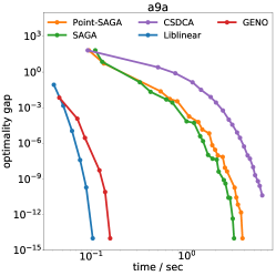
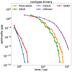
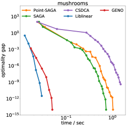
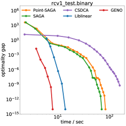
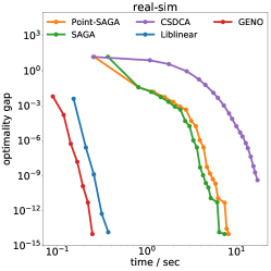
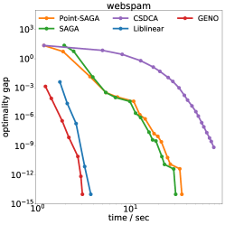
Figure 2: Running times for different solvers on the $\ell_{2}$-regularized logistic regression problem.

On substantially smaller data sets we also compared GENO to CVXPY with both the ECOS [26] and the SCS solver [60]. As can be seen from Table 2, GENO is orders of magnitude faster.

Table 2: Running times in seconds for different general purpose solvers on small instances of the $\ell_{2}$-regularized logistic regression problem. The approximation error is close to $10^{-6}$ for all solvers.

Solver	Data sets
	heart	ionosphere	breast-cancer	australian	diabetes	a1a	a5a
GENO	0.005	0.013	0.004	0.014	0.006	0.023	0.062
ECOS	1.999	2.775	5.080	5.380	5.881	12.606	57.467
SCS	2.589	3.330	6.224	6.578	6.743	16.361	87.904

4.3 Support Vector Machines

Support Vector Machines (SVMs) [19] have been studied intensively and are widely used, especially in combination with kernels [67]. They remain populat, as is indicated by the still rising citation count of the popular and heavily-cited solver LIBSVM [14]. The dual formulation of an SVM is given as the following quadratic optimization problem

$$\begin{array}[]{rl}\min_{a}&\frac{1}{2}(a\odot y)^{\top}K(a\odot y)-\left\|a\right\|_{1}\\ \operatorname{s.t.}&y^{\top}a=0\\ &0\leq a\leq c,\end{array}$$

where $K\in\mathbb{R}^{m\times m}$ is a kernel matrix, $y\in\{-1,+1\}^{m}$ is a binary label vector, $c\in\mathbb{R}$ is the regularization parameter, and $\odot$ is the element-wise multiplication. While the SVM problem with a kernel can also be solved in the primal [15], it is traditionally solved in the dual. We use a Gaussian kernel, i.e., $K_{ij}=\exp\left(-\gamma\left\|X_{i}-X_{j}\right\|_{2}^{2}\right)$ and standard data sets. We set the bandwith parameter $\gamma=1/2$ which corresponds to roughly the median of the pairwise data point distances and set $C=1$. Table 3 shows that the solver generated by GENO is as efficient as LIBSVM which has been maintained and improved over the last 15 years. Both solvers outperform general purpose approaches like CVXPY with OSQP [70], SCS [60], Gurobi [39], or Mosek [56] by a few orders of magnitude.

Table 3: Running times in seconds for solving a dual Gaussian-kernelized SVM. The optimality gap is close to $10^{-4}$ for all solvers and data sets. Missing entries in the table indicate that the solver did not finish within one hour.

Solver	Datasets
	ionosphere	australian	diabetes	a1a	a5a	a9a	w8a	cod-rna
GENO	0.009	0.024	0.039	0.078	1.6	30.0	25.7	102.1
LIBSVM	0.005	0.010	0.009	0.088	1.0	18.0	78.6	193.1
SCS	0.442	1.461	3.416	11.707	517.5	-	-	-
OSQP	0.115	0.425	0.644	3.384	168.2	-	-	-
Gurobi	0.234	0.768	0.992	4.307	184.4	-	-	-
Mosek	0.378	0.957	1.213	6.254	152.7	-	-	-

4.4 Elastic Net

Elastic net regression [76] has also been studied intensively and is used mainly for mircoarray data classification and gene selection. Given some data $X\in\mathbb{R}^{m\times n}$ and a response $y\in\mathbb{R}^{m}$, elastic net regression seeks to minimize

$$\frac{1}{2m}\left\|Xw-y\right\|^{2}_{2}+\alpha\left(\lambda\left\|w\right\|+\frac{1-\lambda}{2}\left\|w\right\|_{2}^{2}\right),$$

where $\alpha$ and $\lambda$ are the corresponding elastic net regularization parameters. The most popular solver is glmnet, a dual coordinate descent approach that has been implementated in Fortran [33]. In our experiments, we follow the same setup as in [33]. We generated Gaussian data $X\in\mathbb{R}^{m\times n}$ with $m$ data points and $n$ features. The outcome values $y$ were generated by

$$y=\sum_{j=1}^{n}X_{j}\beta_{j}+k\cdot z,$$

where $\beta_{j}=(-1)^{j}\exp(-j/10)$, $z\sim{\cal{N}}(0,1)$, and $k$ is chosen such that the signal-to-noise ratio is 3. We varied the number of data points $m$ and the number of features $n$. The results are shown in Table 4. It can be seen that the solver generated by GENO is as efficient as glment and orders of magnitude faster than comparable state-of-the-art general purpose approaches like CVXPY coupled with ECOS, SCS, Gurobi, or Mosek. Note, that the OSQP solver could not be run on this problem since CVXPY raised the error that it cannot convert this problem into a QP.

Table 4: Running times for the elastic net regression problem in seconds. Missing entries in the table indicate that the solver did not finish within one hour. The optimality gap is about $10^{-8}$ for all solvers which is the standard setting for glmnet.

m	n	Solvers
		GENO	glmnet	ECOS	SCS	Gurobi	Mosek
1000	1000	0.11	0.10	43.27	2.33	21.14	1.77
2000	1000	0.14	0.08	202.04	9.24	58.44	3.52
3000	1000	0.18	0.08	513.78	22.86	114.79	5.38
4000	1000	0.21	0.09	-	38.90	185.79	7.15
5000	1000	0.27	0.11	-	13.88	151.08	8.69
1000	5000	1.74	0.62	-	28.69	-	13.06
2000	5000	1.49	1.41	-	45.79	-	27.69
3000	5000	1.58	2.02	-	81.83	-	50.99
4000	5000	1.24	1.88	-	135.94	-	67.60
5000	5000	1.41	1.99	-	166.60	-	71.92
5000	10000	4.11	4.75	-	-	-	-
7000	10000	4.76	5.52	-	-	-	-
10000	10000	4.66	3.89	-	-	-	-
50000	10000	13.97	6.34	-	-	-	-
70000	10000	18.82	11.76	-	-	-	-
100000	10000	23.38	23.42	-	-	-	-

4.5 Non-negative Least Squares

Least squares is probably the most widely used regression method. Non-negative least squares is an extension that requires the output to be non-negative. It is given as the following optimization problem

$$\begin{array}[]{rl}\min_{x}&\left\|Ax-b\right\|_{2}^{2}\\ \operatorname{s.t.}&x\geq 0,\end{array}$$

where $A\in\mathbb{R}^{m\times n}$ is a given design matrix and $b\in\mathbb{R}^{m}$ is the response vector. Since non-negative least squares has been studied intensively, there is a plenitude of solvers available that implement different optimization methods. An overview and comparison of the different methods can be found in [69]. Here, we use the accompanying code described in [69] for our comparison. We ran two sets of experiments, similarly to the comparisons in [69], where it was shown that the different algorithms behave quite differently on these problems. For experiment (i), we generated random data $A\in\mathbb{R}^{2000\times 6000}$, where the entries of $A$ were sampled uniformly at random from the interval $[0,1]$ and a sparse vector $x\in\mathbb{R}^{6000}$ with non-zero entries sampled also from the uniform distribution of $[0,1]$ and a sparsity of $0.01$. The outcome values were then generated by $y=\sqrt{0.003}\cdot Ax+0.003\cdot z$, where $z\sim{\cal{N}}(0,1)$. For experiment (ii), $A\in\mathbb{R}^{6000\times 3000}$ was drawn form a Gaussian distribution and $x$ had a sparsity of $0.1$. The outcome variable was generated by $y=\sqrt{1/6000}\cdot Ax+0.003\cdot z$, where $z\sim{\cal{N}}(0,1)$. The differences between the two experiments are the following: (1) The Gram matrix $A^{\top}A$ is singular in experiment (i) and regular in experiment (ii), (2) The design matrix $A$ has isotropic rows in experiment (ii) which does not hold for experiment (i), and (3) $x$ is significantly sparser in (i) than in (ii). We compared the solver generated by GENO with the following approaches: the classical Lawson-Hanson algorithm [48], which employs an active set strategy, a projected gradient descent algorithm combined with an Armijo-along-projection-arc line search [5, Ch 2.3], a primal-dual interior point algorithm that uses a conjugate gradient descent algorithm [8] with a diagonal preconditioner for solving the Newton system, a subspace Barzilai-Borwein approach [44], and Nesterov’s accelerated projected gradient descent [58]. Figure 3 shows the results for both experiments. Note, that the Barzilai-Borwein approach with standard parameter settings diverged on experiment (i) and it would stop making progress on experiment (ii). While the other approaches vary in running time depending on the problem, the experiments show that the solver generated by GENO is always among the fastest compared to the other approaches.

We provide the final running times of the general purpose solvers in Table 5 since obtaining intermediate solutions is not possible for these solvers. Table 5 also provides the function values of the individual solvers. It can be seen, while the SCS solver is considerably faster than the ECOS solver, the solution computed by the SCS solver is not optimal in experiment (i). The ECOS solver provides a solution with the same accuracy as GENO but at a running time that is a few orders of magnitude larger.

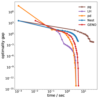
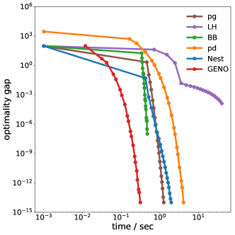
Figure 3: Running times for non-negative least squares regression. The figure on the left shows the running times for the experiment (i) and the figure on the right the running times for experiment (ii). The algorithms are projected gradient descent (pd), Lawson-Hanson (LH), subspace Barzilai-Borwein (BB), primal-dual interior point method (pd), Nesterov’s accelerated projected gradient descent (Nest), and GENO.

Table 5: Running times and function values for the non-negative least squares problem.

m	n		GENO	ECOS	SCS	Gurobi	Mosek
2000	6000	time	4.8	689.7	70.4	187.3	24.9
		fval	0.01306327	0.01306327	0.07116707	0.01306330	0.01306343
6000	3000	time	0.3	3751.3	275.5	492.9	58.4
		fval	0.03999098	0.03999098	0.04000209	0.03999100	0.03999114

4.6 Symmetric Non-negative Matrix Factorization

Non-negative matrix factorization (NMF) and its many variants are standard methods for recommender systems [2] and topic modeling [7, 41]. It is known as symmetric NMF, when both factor matrices are required to be identical. Symmetric NMF is used for clustering problems [46] and known to be equivalent to $k$-means kernel clustering [25]. Given a target matrix $T\in\mathbb{R}^{n\times n}$, symmetric NMF is given as the following optimization problem

$$\min_{U}\>\left\|T-UU^{\top}\right\|_{\mbox{\scriptsize Fro}}^{2}\quad\operatorname{s.t.}\>U\geq 0,$$

where $U\in\mathbb{R}^{n\times k}$ is a positive factor matrix of rank $k$. Note, the problem cannot be modeled and solved by CVXPY since it is non-convex. It has been addressed recently in [74] by two new methods. Both methods are symmetric variants of the alternating non-negative least squares (ANLS) [45] and the hierarchical ALS (HALS) [18] algorithms.

We compared GENO to both methods. For the comparison we used the code and same experimental setup as in [74]. Random positive-semidefinite target matrices $X=\hat{U}\hat{U}^{\top}$ of different sizes were computed from random matrices $\hat{U}\in\mathbb{R}^{n\times k}$ with absolute value Gaussian entries. As can be seen in Figure 4, GENO outperforms both methods (SymANLS and SymHALS) by a large margin.

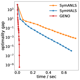
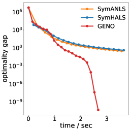
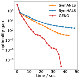
Figure 4: Convergence speed on the symmetric non-negative matrix factorization problem for different parameter values. On the left, the times for $m=50,k=5$, in the middle for $m=500,k=10$, and on the right for $m=2000,k=15$.

4.7 Non-linear Least Squares

GENO makes use of a quasi-Newton solver which approximates the Hessian by the weighted sum of the identity matrix and a positive semidefinite, low-rank matrix. One could assume that this does not work well in case that the true Hessian is indefinite, i.e., in the non-convex case. Hence, we also conducted some experiments on non-convex problems. We followed the same setup and ran the same experiments as in [51] and compared to state-of-the-art solvers that were specifically designed to cope with non-convex problems. Especially, we considered the non-linear least squares problem, i.e., we seek to minimize the function $l(x)=\left\|\sigma(Ax)-b\right\|_{2}^{2}$, where $A\in\mathbb{R}^{m\times n}$ is a data matrix, $y\in\{0,1\}^{m}$ is a binary label vector, and $\sigma(s)=1/(1+\exp(-s))$ is the sigmoid function. Figure 5 shows the convergence speed for the data set w1a and a1a. The state-of-the-art specialized solvers that were introduced in [51] are S-AdaNCG, which is a stochastic adaptive negative curvature and gradient algorithm, and AdaNCD-SCSG, an adaptive negative curvature descent algorithm that uses SCSG [49] as a subroutine. The experiments show that GENO outperforms both algorithms by a large margin. In fact, on the data set a1a, both algorithms would not converge to the optimal solution with standard parameter settings. Again, this problem cannot be modeled and solved by CVXPY.

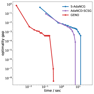
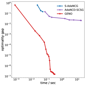
Figure 5: Running times for the non-linear least squares problem. The figure on the left shows the running times for the data set w1a and on the right for the data set a1a.

4.8 Compressed Sensing

In compressed sensing, one tries to recover a sparse signal from a number of measurements [13, 27]. See the recent survey [65] for an overview on this topic. The problem can be reduced to finding the solution to an underdetermined system of linear equations with minimal $\ell_{1}$-norm. Hence, it can be written as the following optimization problem

$$\begin{array}[]{rl}\min_{x}&\left\|x\right\|_{1}\\ \operatorname{s.t.}&Ax=b,\end{array}$$ (2)

where $A\in\mathbb{R}^{m\times n}$ is a measurement matrix and $b\in\mathbb{R}^{m}$ is the vector of $m$ measurements. Note, that this problem is a constrained problem with a non-differentiable objective function. It is known that when matrix $A$ has the restricted isometry property and the true signal $x^{*}$ is sparse, then Problem (2) recovers the true signal with high probability, if the dimensions $m$ and $n$ are chosen properly [12]. There has been made considerable progress in designing algorithms that come with convergence guarantees [16, 17]. Very recently, in [29] a new and efficient algorithm based on the iterative reweighted least squares (IRLS) technique has been proposed. Compared to previous approaches, their algorithm is simple and achieves the state-of-the-art convergence guarantees for this problem.

We used the same setup and random data set as in [29] and ran the same experiment. The measurement matrix $A\in\mathbb{R}^{150\times 200}$ had been generated randomly, such that all rows are orthogonal. Then, a sparse signal $x^{*}$ with only 15 non-zero entries had been chosen and the corresponding measurement vector $b$ had been computed via $b=Ax^{*}$. We compared to their IRLS algorithm with the long-steps update scheme. Figure 6 shows the convergence speed speed towards the optimal function value as well as the convergence towards feasibility. It can be seen that the solver generated by GENO outperforms the specialized, state-of-the-art IRLS solver by a few orders of magnitude.

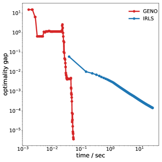
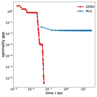
Figure 6: Running times for the compressed sensing problem. The figure on the left shows the convergence to the optimal objective function value and the figure on the right shows the norm of the constraint violation of the iterate $x^{(k)}$, i.e., $\left\|Ax^{(k)}-b\right\|_{2}$.

5 Conclusions

While other fields of applied research that heavily rely on optimization, like operations research, optimal control and deep learning, have adopted optimization frameworks, this is not the case for classical machine learning. Instead, classical machine learning methods are still mostly accessed through toolboxes like scikit-learn, Weka, or MLlib. These toolboxes provide well-engineered solutions for many of the standard problems, but lack the flexibility to adapt the underlying models when necessary. We attribute this state of affairs to a common belief that efficient optimization for classical machine learning needs to exploit the problem structure. Here, we have challenged this belief. We have presented GENO the first general purpose framework for problems from classical machine learning. GENO combines an easy-to-read modeling language with a general purpose solver. Experiments on a variety of problems from classical machine learning demonstrate that GENO is as efficient as established well-engineered solvers and often outperforms recently published state-of-the-art solvers by a good margin. It is as flexible as state-of-the-art modeling language and solver frameworks, but outperforms them by a few orders of magnitude.

Appendix

Appendix A GENO Models for all Experiments

 

   

 parameters 

    Matrix X 

    Scalar c 

    Vector y 

 variables 

    Scalar b 

    Vector w 

 min 

    norm1(w) + c 

    * sum(log(exp((-y) .* (X*w 

    + vector(b))) + vector(1))) 

   

 

Figure 7: $\ell_{1}$-regularized Logistic Regression

 

   

 parameters 

    Matrix X 

    Scalar c 

    Vector y 

 variables 

    Vector w 

 min 

    0.5 * w’ * w 

    + c * sum(log(exp((-y) .* (X * w)) 

    + vector(1))) 

  

   

 

Figure 8: $\ell_{2}$-regularized Logistic Regression

 

   

 parameters 

    Matrix K symmetric 

    Scalar c 

    Vector y 

 variables 

    Vector a 

 min 

    0.5 * (a.*y)’ * K * (a.*y) - sum(a) 

 st 

    a >= 0 

    y’ * a == 0 

   

 

Figure 9: Support Vector Machine

 

   

 parameters 

    Matrix X 

    Scalar a1 

    Scalar a2 

    Scalar n 

    Vector y 

 variables 

    Vector w 

 min 

    n * norm2(X*w - y).^2 

    + a1 * norm1(w) + a2 * w’ * w 

   

 

Figure 10: Elastic Net

 

   

 parameters 

    Matrix A 

    Vector b 

 variables 

    Vector x 

 min 

    norm2(A*x - b).^2 

 st 

    x > 0 

   

 

Figure 11: Non-negative Least Squares

 

   

 parameters 

    Matrix X symmetric 

 variables 

    Matrix U 

 min 

    norm2(X - U*U’).^2 

 st 

    U >= 0 

  

   

 

Figure 12: Symmetric NMF

 

   

 parameters 

    Matrix X 

    Scalar s 

    Vector y 

 variables 

    Vector w 

 min 

    s * norm2(y - 0.5 

    * tanh(0.5 * X * w) 

    + vector(0.5)).^2 

   

 

Figure 13: Non-linear Least Squares

 

   

 parameters 

    Matrix A 

    Vector b 

 variables 

    Vector x 

 min 

    norm1(x) 

 st 

    A*x == b 

  

   

 

Figure 14: Compressed Sensing

Appendix B Summary of Solvers

Table 6: Summary of all solvers that were used in the experiments.

Name	Type	Reference
GENO	quasi-Newton w/ augmented Lagrangian	this paper
OSQP	ADMM	[70]
SCS	ADMM	[60]
ECOS	interior point	[26]
Gurobi	interior point	[39]
Mosek	interior point	[56]
LIBSVM	Frank-Wolfe (SMO)	[14]
LIBLINEAR	conjugate gradient +	[30, 75]
	dual coordinate descent
SAGA	SGD	[23]
SDCA	SGD	[68]
catalyst SDCA	SGD	[50]
Point-SAGA	SGD	[22]
glmnet	dual coordinate descent	[33]
Lawson-Hanson	direct linear equations solver w/ active set	[48]
projected gradient descent	proximal algorithm	[69]
primal-dual interior point w/	interior point	[69]
preconditioned conjugate gradient
subspace Barlizai-Borwein	quasi-Newton	[44]
Nesterov’s method	accelerated gradient descent	[58]
SymANLS	block coordinate descent	[74]
SymHALS	block coordinate descent	[74]
S-AdaNCG	SGD	[51]
AdaNCD-SCSG	SGD	[51]
IRLS	IRLS w/ conjugate gradient method	[29]

References

- [1] Martín Abadi, Paul Barham, Jianmin Chen, Zhifeng Chen, Andy Davis, Jeffrey Dean, Matthieu Devin, Sanjay Ghemawat, Geoffrey Irving, Michael Isard, Manjunath Kudlur, Josh Levenberg, Rajat Monga, Sherry Moore, Derek G. Murray, Benoit Steiner, Paul Tucker, Vijay Vasudevan, Pete Warden, Martin Wicke, Yuan Yu, and Xiaoqiang Zheng. TensorFlow: A system for large-scale machine learning. In USENIX Conference on Operating Systems Design and Implementation (OSDI), pages 265–283, 2016.
- [2] Gediminas Adomavicius and Alexander Tuzhilin. Toward the next generation of recommender systems: A survey of the state-of-the-art and possible extensions. IEEE Transactions on Knowledge & Data Engineering, (6):734–749, 2005.
- [3] Akshay Agrawal, Robin Verschueren, Steven Diamond, and Stephen Boyd. A rewriting system for convex optimization problems. Journal of Control and Decision, 5(1):42–60, 2018.
- [4] Goran Banjac, Bartolomeo Stellato, Nicholas Moehle, Paul Goulart, Alberto Bemporad, and Stephen P. Boyd. Embedded code generation using the OSQP solver. In Conference on Decision and Control, (CDC), pages 1906–1911, 2017.
- [5] Dimitri P. Bertsekas. Nonlinear Programming. Athena Scientific, Belmont, MA, 1999.
- [6] Ernesto G. Birgin and José Mario Martínez. Practical augmented Lagrangian methods for constrained optimization, volume 10 of Fundamentals of Algorithms. SIAM, 2014.
- [7] David M Blei, Andrew Y Ng, and Michael I Jordan. Latent dirichlet allocation. Journal of Machine Learning Research, 3(Jan):993–1022, 2003.
- [8] Stephen Boyd and Lieven Vandenberghe. Convex Optimization. Cambridge University Press, New York, NY, USA, 2004.
- [9] Stephen P. Boyd, Neal Parikh, Eric Chu, Borja Peleato, and Jonathan Eckstein. Distributed optimization and statistical learning via the alternating direction method of multipliers. Foundations and Trends in Machine Learning, 3(1):1–122, 2011.
- [10] A. Brooke, D. Kendrick, and A. Meeraus. GAMS: release 2.25 : a user’s guide. The Scientific press series. Scientific Press, 1992.
- [11] Richard H. Byrd, Peihuang Lu, Jorge Nocedal, and Ciyou Zhu. A limited memory algorithm for bound constrained optimization. SIAM J. Scientific Computing, 16(5):1190–1208, 1995.
- [12] Emmanuel J Candès and Terence Tao. Decoding by linear programming. IEEE Transactions on Information Theory, 51(12):4203–4215, 2005.
- [13] Emmanuel J. Candès and Terence Tao. Near-optimal signal recovery from random projections: Universal encoding strategies? IEEE Trans. Information Theory, 52(12):5406–5425, 2006.
- [14] Chih-Chung Chang and Chih-Jen Lin. LIBSVM: A library for support vector machines. ACM Transactions on Intelligent Systems and Technology, 2:27:1–27:27, 2011.
- [15] Olivier Chapelle. Training a support vector machine in the primal. Neural Computation, 19(5):1155–1178, 2007.
- [16] Hui Han Chin, Aleksander Madry, Gary L Miller, and Richard Peng. Runtime guarantees for regression problems. In Conference on Innovations in Theoretical Computer Science (ITCS), pages 269–282, 2013.
- [17] Paul Christiano, Jonathan A Kelner, Aleksander Madry, Daniel A Spielman, and Shang-Hua Teng. Electrical flows, laplacian systems, and faster approximation of maximum flow in undirected graphs. In ACM Symposium on Theory of Computing (STOC), pages 273–282, 2011.
- [18] Andrzej Cichocki and Anh-Huy Phan. Fast local algorithms for large scale nonnegative matrix and tensor factorizations. Transactions on Fundamentals of Electronics, Communications and Computer Sciences, 92(3):708–721, 2009.
- [19] Corinna Cortes and Vladimir Vapnik. Support-vector networks. Machine Learning, 20(3):273–297, 1995.
- [20] David R. Cox. The regression analysis of binary sequences (with discussion). J. Roy. Stat. Soc. B, 20:215–242, 1958.
- [21] CVX Research, Inc. CVX: Matlab software for disciplined convex programming, version 2.1. http://cvxr.com/cvx, December 2018.
- [22] Aaron Defazio. A simple practical accelerated method for finite sums. In Advances in Neural Information Processing Systems (NIPS), pages 676–684, 2016.
- [23] Aaron Defazio, Francis R. Bach, and Simon Lacoste-Julien. SAGA: A fast incremental gradient method with support for non-strongly convex composite objectives. In Advances in Neural Information Processing Systems (NIPS), pages 1646–1654, 2014.
- [24] Steven Diamond and Stephen Boyd. CVXPY: A Python-embedded modeling language for convex optimization. Journal of Machine Learning Research, 17(83):1–5, 2016.
- [25] Chris Ding, Xiaofeng He, and Horst D Simon. On the equivalence of nonnegative matrix factorization and spectral clustering. In SIAM International Conference on Data Mining (SDM), pages 606–610. SIAM, 2005.
- [26] Alexander Domahidi, Eric Chu, and Stephen P. Boyd. ECOS: An SOCP Solver for Embedded Systems. In European Control Conference (ECC), 2013.
- [27] David Donoho. Compressed sensing. IEEE Transactions on Information Theory, 52(4):1289–1306, 2006.
- [28] Iain Dunning, Joey Huchette, and Miles Lubin. JuMP: A modeling language for mathematical optimization. SIAM Review, 59(2):295–320, 2017.
- [29] Alina Ene and Adrian Vladu. Improved convergence for and regression via iteratively reweighted least squares. In International Conference on Machine Learning (ICML), 2019. To appear.
- [30] Rong-En Fan, Kai-Wei Chang, Cho-Jui Hsieh, Xiang-Rui Wang, and Chih-Jen Lin. LIBLINEAR: A library for large linear classification. Journal of Machine Learning Research, 9:1871–1874, 2008.
- [31] Robert Fourer, David M. Gay, and Brian W. Kernighan. AMPL: a modeling language for mathematical programming. Thomson/Brooks/Cole, 2003.
- [32] Eibe Frank, Mark A. Hall, and Ian H. Witten. The WEKA Workbench. Online Appendix for "Data Mining: Practical Machine Learning Tools and Techniques”. Morgan Kaufmann, fourth edition, 2016.
- [33] Jerome H. Friedman, Trevor Hastie, and Rob Tibshirani. Regularization paths for generalized linear models via coordinate descent. Journal of Statistical Software, 33(1):1–22, 2010.
- [34] Daniel Gabay and Bertrand Mercier. A dual algorithm for the solution of nonlinear variational problems via finite element approximation. Computers & Mathematics with Applications, 2(1):17 – 40, 1976.
- [35] P. Giselsson and S. Boyd. Linear convergence and metric selection for Douglas-Rachford splitting and ADMM. IEEE Transactions on Automatic Control, 62(2):532–544, Feb 2017.
- [36] R. Glowinski and A. Marroco. Sur l’approximation, par éléments finis d’ordre un, et la résolution, par pénalisation-dualité d’une classe de problèmes de dirichlet non linéaires. ESAIM: Mathematical Modelling and Numerical Analysis - Modélisation Mathématique et Analyse Numérique, 9(R2):41–76, 1975.
- [37] Jean-Louis Goffin. On convergence rates of subgradient optimization methods. Math. Program., 13(1):329–347, 1977.
- [38] M. Grant and S. Boyd. Graph implementations for nonsmooth convex programs. In V. Blondel, S. Boyd, and H. Kimura, editors, Recent Advances in Learning and Control, Lecture Notes in Control and Information Sciences, pages 95–110. 2008.
- [39] Gurobi Optimization, Inc. Gurobi Optimizer. http://www.gurobi.com.
- [40] Magnus R. Hestenes. Multiplier and gradient methods. Journal of Optimization Theory and Applications, 4(5):303–320, 1969.
- [41] Thomas Hofmann. Probabilistic latent semantic analysis. In Conference on Uncertainty in Artificial Intelligence (UAI), pages 289–296, 1999.
- [42] Ho-Yi Huang. Unified approach to quadratically convergent algorithms for function minimization. Journal of Optimization Theory and Applications, 5(6):405–423, 1970.
- [43] Yangqing Jia, Evan Shelhamer, Jeff Donahue, Sergey Karayev, Jonathan Long, Ross Girshick, Sergio Guadarrama, and Trevor Darrell. Caffe: Convolutional architecture for fast feature embedding. arXiv preprint arXiv:1408.5093, 2014.
- [44] Dongmin Kim, Suvrit Sra, and Inderjit S Dhillon. A non-monotonic method for large-scale non-negative least squares. Optimization Methods and Software, 28(5):1012–1039, 2013.
- [45] Jingu Kim and Haesun Park. Toward faster nonnegative matrix factorization: A new algorithm and comparisons. In IEEE International Conference on Data Mining (ICDM), pages 353–362, 2008.
- [46] Da Kuang, Sangwoon Yun, and Haesun Park. Symnmf: nonnegative low-rank approximation of a similarity matrix for graph clustering. Journal of Global Optimization, 62(3):545–574, 2015.
- [47] Sören Laue, Matthias Mitterreiter, and Joachim Giesen. Computing higher order derivatives of matrix and tensor expressions. In Advances in Neural Information Processing Systems (NeurIPS), 2018.
- [48] Charles L. Lawson and Richard J. Hanson. Solving least squares problems. Classics in Applied Mathematics. SIAM, 1995.
- [49] Lihua Lei, Cheng Ju, Jianbo Chen, and Michael I Jordan. Non-convex finite-sum optimization via scsg methods. In Advances in Neural Information Processing Systems, pages 2348–2358, 2017.
- [50] Hongzhou Lin, Julien Mairal, and Zaïd Harchaoui. A universal catalyst for first-order optimization. In Advances in Neural Information Processing Systems (NIPS), pages 3384–3392, 2015.
- [51] Mingrui Liu, Zhe Li, Xiaoyu Wang, Jinfeng Yi, and Tianbao Yang. Adaptive negative curvature descent with applications in non-convex optimization. In Advances in Neural Information Processing Systems (NeurIPS), pages 4858–4867, 2018.
- [52] Jacob Mattingley and Stephen Boyd. CVXGEN: A Code Generator for Embedded Convex Optimization. Optimization and Engineering, 13(1):1–27, 2012.
- [53] Xiangrui Meng, Joseph Bradley, Burak Yavuz, Evan Sparks, Shivaram Venkataraman, Davies Liu, Jeremy Freeman, DB Tsai, Manish Amde, Sean Owen, Doris Xin, Reynold Xin, Michael J. Franklin, Reza Zadeh, Matei Zaharia, and Ameet Talwalkar. Mllib: Machine learning in apache spark. Journal of Machine Learning Research, 17(1), January 2016.
- [54] José Luis Morales and Jorge Nocedal. Remark on "algorithm 778: L-BFGS-B: fortran subroutines for large-scale bound constrained optimization". ACM Trans. Math. Softw., 38(1):7:1–7:4, 2011.
- [55] Jorge J. Moré and David J. Thuente. Line search algorithms with guaranteed sufficient decrease. ACM Trans. Math. Softw., 20(3):286–307, 1994.
- [56] MOSEK ApS. The MOSEK optimization software. http://www.mosek.com.
- [57] L. Nazareth. A relationship between the bfgs and conjugate gradient algorithms and its implications for new algorithms. SIAM Journal on Numerical Analysis, 16(5):794–800, 1979.
- [58] Yurii Nesterov. A method for unconstrained convex minimization problem with the rate of convergence . Doklady AN USSR (translated as Soviet Math. Docl.), 269, 1983.
- [59] Yurii Nesterov. Smooth minimization of non-smooth functions. Math. Program., 103(1):127–152, 2005.
- [60] Brendan O’Donoghue, Eric Chu, Neal Parikh, and Stephen Boyd. Conic optimization via operator splitting and homogeneous self-dual embedding. Journal of Optimization Theory and Applications, 169(3):1042–1068, 2016.
- [61] Adam Paszke, Sam Gross, Soumith Chintala, Gregory Chanan, Edward Yang, Zachary DeVito, Zeming Lin, Alban Desmaison, Luca Antiga, and Adam Lerer. Automatic differentiation in pytorch. In NIPS Autodiff workshop, 2017.
- [62] F. Pedregosa, G. Varoquaux, A. Gramfort, V. Michel, B. Thirion, O. Grisel, M. Blondel, P. Prettenhofer, R. Weiss, V. Dubourg, J. Vanderplas, A. Passos, D. Cournapeau, M. Brucher, M. Perrot, and E. Duchesnay. Scikit-learn: Machine learning in Python. Journal of Machine Learning Research, 12:2825–2830, 2011.
- [63] Nicholas G. Polson, James G. Scott, and Brandon T. Willard. Proximal algorithms in statistics and machine learning. arXiv preprint, May 2015.
- [64] M. J. D. Powell. Algorithms for nonlinear constraints that use Lagrangian functions. Mathematical Programming, 14(1):224–248, 1969.
- [65] Meenu Rani, S. B. Dhok, and R. B. Deshmukh. A systematic review of compressive sensing: Concepts, implementations and applications. IEEE Access, 6:4875–4894, 2018.
- [66] Herbert Robbins and Sutton Monro. A stochastic approximation method. Ann. Math. Statist., 22(3):400–407, 1951.
- [67] Bernhard Schölkopf and Alexander J. Smola. Learning with Kernels: Support Vector Machines, Regularization, Optimization, and Beyond. MIT Press, Cambridge, MA, USA, 2001.
- [68] Shai Shalev-Shwartz and Tong Zhang. Stochastic dual coordinate ascent methods for regularized loss. Journal of Machine Learning Research, 14(1):567–599, 2013.
- [69] Martin Slawski. Problem-specific analysis of non-negative least squares solvers with a focus on instances with sparse solutions. https://sites.google.com/site/slawskimartin/code, March 2013.
- [70] B. Stellato, G. Banjac, P. Goulart, A. Bemporad, and S. Boyd. OSQP: An operator splitting solver for quadratic programs. arXiv preprint, November 2017.
- [71] P. Wolfe. Convergence conditions for ascent methods. SIAM Review, 11(2):226–235, 1969.
- [72] P. Wolfe. Convergence conditions for ascent methods. ii: Some corrections. SIAM Review, 13(2):185–188, 1971.
- [73] Ciyou Zhu, Richard H. Byrd, Peihuang Lu, and Jorge Nocedal. Algorithm 778: L-BFGS-B: fortran subroutines for large-scale bound-constrained optimization. ACM Trans. Math. Softw., 23(4):550–560, 1997.
- [74] Zhihui Zhu, Xiao Li, Kai Liu, and Qiuwei Li. Dropping symmetry for fast symmetric nonnegative matrix factorization. In Advances in Neural Information Processing Systems (NeurIPS), pages 5160–5170, 2018.
- [75] Yong Zhuang, Yu-Chin Juan, Guo-Xun Yuan, and Chih-Jen Lin. Naive parallelization of coordinate descent methods and an application on multi-core l1-regularized classification. In International Conference on Information and Knowledge Management (CIKM), pages 1103–1112, 2018.
- [76] Hui Zou and Trevor Hastie. Regularization and variable selection via the elastic net. Journal of the Royal Statistical Society, Series B, 67:301–320, 2005.