Abstract

The self coupling $\lambda$ of the Higgs boson in the Standard Model may show critical behavior, i.e. the Higgs potential may have a point at an energy scale $\sim 10^{17-18}$ GeV where both the first and second derivatives (almost) vanish. In this case the Higgs boson can serve as inflaton even if its nonminimal coupling to the curvature scalar is only ${\cal O}(10)$, thereby alleviating concerns about the perturbative unitarity of the theory. We find that just before the Higgs as inflaton enters the flat region of the potential the usual slow–roll conditions are violated. This leads to “overshooting” behavior, which in turn strongly enhances scalar curvature perturbations because of the excitation of entropic (non–adiabatic) perturbations. For appropriate choice of the free parameters these large perturbations occur at length scales relevant for the formation of primordial black holes. Even if these perturbations are not quite large enough to trigger copious black hole formation, they source second order tensor perturbations, i.e. primordial gravitational waves; the corresponding energy density can be detected by the proposed space-based gravitational wave detectors DECIGO and BBO.

1 Introduction

Inflation is a beautiful paradigm for the evolution of the very early universe: it not only solves the problems of standard cosmology [1, 2, 3], but also generates the initial seeds for the formation of large structures via quantum fluctuations. The simplest inflationary models feature a single scalar field that slowly “rolls down” a rather flat potential (“slow–roll” inflation). The energy density during inflation is then dominated by the potential, which leads to an approximately exponential expansion of the universe. Often a separate “inflaton” field is introduced for this purpose, but it would obviously be more economical to instead use the single scalar Higgs field $\Phi$ of the Standard Model (SM) of particle physics as inflaton. At TeV energies the Higgs self coupling $\lambda$ is ${\cal O}(0.1)$; a coupling of this size leads to a rather steep potential, which needs to be “flattened” by a large non–minimal coupling to the Ricci scalar, $\xi\Phi^{\dagger}\Phi R$ [4]. This yields [4, 5, 6, 7, 8, 9, 10] $n_{s}\simeq 0.97,r\simeq 0.0034$ in agreement with observation, but for a coupling $\xi\sim 10^{4}$. Such a large coupling may violate perturbative unitarity cutoff [12, 13, 14].

This unitarity issue has been discussed at length in the literature [15, 16, 17, 18, 19, 20, 21, 22, 23, 24, 25]. In particular, it is argued in [15] that the unitarity bound could be higher than the inflationary scale if the inflaton field background is taken into account in the effective field theory (EFT) setup. However it is shown that unitarity would still be violated due to the violent production of longitudinal gauge bosons during preheating, where modes with momenta (much) higher than the perturbative cutoff (even with the background field) can be excited [23, 24, 25] . So unitarity would still be an issue in the post-inflationary phase even though it is not during inflation. This has motivated extensions of original scenario to some UV completed theory by considering Higgs inflation with additional field(s) beyond the SM [26, 27, 28, 29, 30, 31, 32, 33]; however, these models lack the simplicity of the original suggestion.

On the other hand, at the large field values where Higgs inflation may have occurred, the value of $\lambda$ is expected to be quite different than at the weak scale. This difference is described by renormalization group equations (RGE). At the one–loop order $\lambda$ is driven to larger values by Higgs self–interactions (i.e. the $\lambda^{2}$ term contributes with positive sign in the RGE) and by electroweak gauge interactions, but is reduced by Yukawa interactions, the by far most important one being that of the top. The evolution of the top Yukawa coupling in turn is also affected by QCD interactions. For the measured value of the mass of the physical Higgs boson (which determines $\lambda$ at the electroweak energy scale), the two–loop RGE indicate that $\lambda$ may show critical behavior at energy scale $\sim 10^{17-18}$ GeV, i.e. $\lambda$ and its first derivative, described by its beta function, can both be very small [36]. This implies that the potential becomes very flat in this region [38], which can give rise to “critical Higgs inflation” (CHI). Since $\lambda$ is small, one only needs a non–minimal coupling $\xi\sim\mathcal{O}(10)$[41, 42, 43]; see also [44, 45, 46, 47] for recent investigations concerning CHI and [48] for a comprehensive review of Higgs inflation.

In addition to reproducing the measured CMB power spectrum accurately, recently some other cosmological implications of the CHI scenario have been investigated. In particular ref. [49] showed that curvature perturbations are greatly enhanced at the length scales that leave the horizon when the inflaton field enters the very flat region of the potential; this might even lead to the formation of a cosmologically significant abundance of primordial black holes (PBH). In fact, in the simplest approximation the strength of the density perturbations is inversely proportional to the first derivative $V^{\prime}$ of the inflaton potential $V$. It is thus tempting to associate a spike in the spectrum of density perturbations with an “ultra–slow roll” (USR) phase in which the inflaton field moves extremely slowly because it traverses a very flat piece of the potential. We will see in Section 2 that this is not the whole story: the largest enhancement actually does not happen in the USR phase, but during a transitionary “overshooting” stage just before USR where the inflaton potential has a sizable curvature, so that the slow–roll (SR) conditions are violated. We will show that in this case curvature perturbations can continue to grow even after they cross out of the horizon, since the perturbations are no longer adiabatic, i.e. “entropic” perturbations are excited. To our knowledge, this is the first investigation of significant effects due entropic perturbations on observable inhomogeneities.

The enhanced scalar curvature perturbations are expected to source tensor perturbations at second order, as investigated in recent papers [51, 66, 67, 68, 69, 70, 71, 72, 73, 74]. In this paper, we improve and further extend the analysis in [49] in several ways. First of all, the power spectrum in [49] is calculated within the SR approximation at all scales; however this assumption does not hold during the overshooting phase. We therefore use the more accurate numerical Mukhanov–Sasaki formalism. Moreover, detailed explanations for our numerical results for the power spectrum are given; this might help to understand features of the power spectrum in other PBH production scenarios from single field inflation with a near–inflection point, for example [51, 59, 63]. With a more realistic result of scalar power spectrum, we investigate the second order gravitational wave (GW) signatures arising from large scalar curvature perturbations in the CHI scenario. We show that such signatures can be detected by several proposed space based GW experiments. The calculation of the PBH density is fraught with considerable uncertainty [75, 76]. Our result indicates that, at least for CHI inflation, an inflationary GW signal should be detectable in all cases that could conceivably lead to sizable PBH production, i.e. a failure to detect the latter in future experiments would exclude the possibility that PBHs contribute significantly to cosmological dark matter.

The reminder of this paper is organized as follows. We first revisit the curvature perturbations under adiabatic and non–adiabatic conditions in Section 2; in particular, we show that for non–adiabatic conditions the amplitude of curvature perturbations does not necessarily remain constant after horizon crossing, in contrast to the usual SR treatment. In Section 3 we set up the CHI scenario. Using the general Mukhanov–Sasaki formalism to compute the power spectrum, we show that the standard SR approximation to calculate the power spectrum fails when the inflaton enters an overshooting phase, even if we use “Hubble” rather than “potential” SR parameters. In Section 4 we discuss second order GW signatures induced by the scalar curvature perturbations. Finally we summarize our results in Section 5. In appendix A we give a quick review of the Mukhanov–Sasaki equation and its analytical solution for a (quasi) de Sitter spacetime.

2 Evolution of Curvature Perturbations

2.1 Adiabatic and Entropic Perturbations

In single field SR inflation the quantum fluctuations are adiabatic. As a result the perturbations of all inflaton field dependent quantities $X_{i}$ share the same phase trajectory [77]:

$$\frac{\delta X_{i}(t,\bm{x})}{\dot{\bar{X}}_{i}}=\frac{\delta X_{j}(t,\bm{x})}{\dot{\bar{X}}_{j}}=...=\delta t(\bm{x}),$$ (1)

where $i,j$ denote different observables, $\bar{X}_{i}$ represents the average (background) of $X_{i}$, $\delta X_{i}\equiv X_{i}-\bar{X}_{i}$ its perturbation, and $\dot{\bar{X}}$ the time derivative. In particular, using $X_{1}=p$ (pressure) and $X_{2}=\rho$ (energy density), adiabatic perturbations satisfy

$$\frac{\delta p_{\rm ad}}{\dot{\bar{p}}}=\frac{\delta\rho_{\rm ad}}{\dot{\bar{\rho}}}\Rightarrow\delta p_{\rm ad}\equiv\frac{\dot{\bar{p}}}{\dot{\bar{\rho}}}\delta\rho_{\rm ad}.$$ (2)

Energy density and pressure are defined via the energy–momentum tensor $T_{\mu}^{\nu}$, with $\rho=T_{0}^{0}$ and $p=-\sum_{i=1}^{3}T_{i}^{i}/3$.

However, in some cases the perturbation may not be adiabatic, for example when there are multiple fields interacting with the inflaton [78] or while the universe undergoes a non–SR inflationary phase, see Sec. 2.2. Thus more generally the pressure perturbation can be decomposed into an adiabatic part and an entropic (i.e. non–adiabatic) one:

$$\delta p=\delta p_{\rm ad}+\delta p_{\rm en},$$ (3)

i.e. $\delta p_{\rm en}\equiv\delta p-\delta p_{\rm ad}$. We will show in the next subsection that this distinction has significant impact on the evolution of curvature perturbations.

2.2 Evolution of Curvature Perturbations in SR, USR and Overshooting Phases

In order to relate inflationary predictions and cosmic microwave background (CMB) measurements the gauge invariant scalar quantity called curvature perturbation is usually introduced; it is defined by [79, 80]

$$-\zeta(t,\bm{x})\equiv\Psi(t,\bm{x})+\frac{H}{\dot{\bar{\rho}}(t)}\delta{\rho}(t,\bm{x})\,.$$ (4)

Here $H$ denotes the Hubble parameter, and $\Psi(t,\mathbf{x})$ is a scalar function of coordinates. Physically $\zeta$ represents the spatial curvature of hypersurfaces with uniform energy density [81]. Since the power of the two–point correlation function of $\zeta$ is related to the CMB temperature anisotropies, one has to compute the power spectrum of $\zeta$ for a given inflationary model. This is usually done in Fourier space, where $\zeta(t,\bm{k})$ is associated to perturbations at a comoving length scale $1/k$ with $k=|\bm{k}|$. As we will review below, under SR conditions the power spectrum can be computed when some mode $k$ crosses the horizon, since $\zeta$ is frozen at super–horizon scale, i.e. it remains constant once $k\ll aH$ where $a$ is the (dimensionless) scale factor in the Friedman–Robertson–Walker (FRW) metric. However, whenever the universe deviates from SR expansion, we must in general take the super–horizon evolution of $\zeta$ into account; unfortunately this considerably complicates the accurate computation of the power spectrum.

Using energy-momentum conservation it can be shown that the evolution of $\zeta$ is given by [81]

$$\dot{\zeta}=-H\frac{\delta p_{\rm en}}{\bar{\rho}+\bar{p}}-\Pi\,.$$ (5)

Here $\delta p_{\rm en}$ is the non–adiabatic component of the pressure perturbation, and $\Pi$ is defined as

$$\frac{\Pi}{H}=-\frac{k^{2}}{3a^{2}H^{2}}\left[\zeta-\Psi_{B}\left(1-\frac{2\bar{\rho}}{9(\bar{\rho}+\bar{p})}\frac{k^{2}}{a^{2}H^{2}}\right)\right]\,,$$ (6)

where $\Psi_{B}$ is a Bardeen potential [79] which does not depend on $k$. We thus see that at super horizon scales, i.e. for $k\ll aH$, the second term in eq.(5) can be neglected. If in addition the perturbations are adiabatic, i.e. if $\delta p_{\rm en}$ can be neglected, then $\zeta$ is conserved on super–horizon scales. Weinberg showed [82] that solutions with $\delta p_{\rm en}=0$, and hence $\dot{\zeta}\rightarrow 0$ for $k\ll aH$, always exist. We will see that this is the only solution if the universe follows a SR expansion, i.e. for a quasi–de Sitter spacetime; however, under overshooting conditions a non–adiabatic solution also exists, and can lead to large enhancement of the curvature perturbation.

Since we define $\delta X=X(\phi)-X(\bar{\phi})$, $\delta X$ can include terms that are of higher order in the field perturbation $\delta\phi$. We assume that only a single (inflaton) field $\phi$ has sizable perturbations. Moreover, we are interested only in super–horizon modes where all gradient terms can be neglected. The energy density and pressure are thus given by

$$\rho=\frac{1}{2}\left(\dot{\phi}\right)^{2}+V(\phi)\,;\ \ \ \ p=\frac{1}{2}\left(\dot{\phi}\right)^{2}-V(\phi)\,.$$ (7)

The same equations also describe $\bar{\rho}$ and $\bar{p}$, which $\phi\rightarrow\bar{\phi}$ on the right–hand side. Super–horizon size non–adiabatic pressure perturbations are then given by:

$$\begin{split}\delta p_{\rm en}&=\delta p-\frac{\dot{\bar{p}}}{\dot{\bar{\rho}}}\delta\rho\\ &=\left[\left(\frac{1}{2}\dot{\phi}^{2}-V(\phi)\right)-\left(\frac{1}{2}(\dot{\bar{\phi}})^{2}-V(\bar{\phi})\right)\right]\\ &-\frac{\dot{\bar{\phi}}\ddot{\bar{\phi}}-\dot{\bar{\phi}}V^{\prime}_{\bar{\phi}}}{\dot{\bar{\phi}}\ddot{\bar{\phi}}+\dot{\bar{\phi}}V^{\prime}_{\bar{\phi}}}\left[\left(\frac{1}{2}\dot{\phi}^{2}+V(\phi)\right)-\left(\frac{1}{2}(\dot{\bar{\phi}})^{2}+V(\bar{\phi})\right)\right]\\ &=\left[\frac{1}{2}\left(\dot{\bar{\phi}}+\delta\dot{\phi}\right)^{2}-V(\bar{\phi}+\delta\phi)-\left(\frac{1}{2}(\dot{\bar{\phi}})^{2}-V(\bar{\phi})\right)\right]\\ &-\frac{\ddot{\bar{\phi}}-V^{\prime}_{\bar{\phi}}}{\ddot{\bar{\phi}}+V^{\prime}_{\bar{\phi}}}\left[\frac{1}{2}\left(\dot{\bar{\phi}}+\delta\dot{\phi}\right)^{2}+V(\bar{\phi}+\delta\phi)-\left(\frac{1}{2}(\dot{\bar{\phi}})^{2}+V(\bar{\phi})\right)\right]\,.\end{split}$$ (8)

Using Taylor expansion for the potential up to second order of $\delta\phi$ , we obtain $V(\bar{\phi}+\delta\phi)=V(\bar{\phi})+V^{\prime}_{\bar{\phi}}\delta\phi+\frac{1}{2}V^{\prime\prime}_{\bar{\phi}}(\delta\phi)^{2}$, where $V^{\prime}_{\bar{\phi}}$ denotes $dV(\bar{\phi})/d\bar{\phi}$. Using this expansion, eq.(8) becomes

$$\begin{split}\delta p_{\rm en}&=\left(\dot{\bar{\phi}}\delta\dot{\phi}+\frac{1}{2}(\delta\dot{\phi})^{2}-V^{\prime}_{\bar{\phi}}\delta\phi-\frac{1}{2}V^{\prime\prime}_{\bar{\phi}}(\delta\phi)^{2}\right)\\ &-\frac{\ddot{\bar{\phi}}-V^{\prime}_{\bar{\phi}}}{\ddot{\bar{\phi}}+V^{\prime}_{\bar{\phi}}}\left(\dot{\bar{\phi}}\delta\dot{\phi}+\frac{1}{2}(\delta\dot{\phi})^{2}+V^{\prime}_{\bar{\phi}}\delta\phi+\frac{1}{2}V^{\prime\prime}_{\bar{\phi}}(\delta\phi)^{2}\right)\,.\end{split}$$ (9)

For a strict de Sitter spacetime $V$ has to be constant, i.e. all derivatives of $V$ vanish. It is easy to see that $\delta p_{\rm en}=0$ in this case. However, during realistic SR inflation, $|\ddot{\bar{\phi}}|\ll\left|V^{\prime}_{\bar{\phi}}\right|$, so that eq.(9) reduces to

$$\begin{split}\delta p_{\rm en}&=\left(\dot{\bar{\phi}}\delta\dot{\phi}+\frac{1}{2}(\delta\dot{\phi})^{2}-V^{\prime}_{\bar{\phi}}\delta\phi-\frac{1}{2}V^{\prime\prime}_{\bar{\phi}}(\delta\phi)^{2}\right)\\ &-(-)\left(\dot{\bar{\phi}}\delta\dot{\phi}+\frac{1}{2}(\delta\dot{\phi})^{2}+V^{\prime}_{\bar{\phi}}\delta\phi+\frac{1}{2}V^{\prime\prime}_{\bar{\phi}}(\delta\phi)^{2}\right)\\ &=2\dot{\bar{\phi}}\delta\dot{\phi}+(\delta\dot{\phi})^{2}\,.\end{split}$$ (10)

In order to see that $\delta p_{\rm en}$ is indeed very small during SR, consider the equation of motion for $\delta\phi$ [77, 83]:

$$\delta\ddot{\phi}+3H\delta\dot{\phi}-\frac{\nabla^{2}\delta\phi}{a^{2}}+V^{\prime\prime}\delta\phi=0\,.$$ (11)

In momentum space this becomes

$$\delta\ddot{\phi}_{k}+3H\delta\dot{\phi}_{k}+\frac{k^{2}}{a^{2}}\delta\phi_{k}+V^{\prime\prime}\delta\phi_{k}=0\,.$$ (12)

In analyses of inflationary dynamics it is often useful to trade the time for the number of e–folds $N$ via $dN=Hdt$; eq.(12) then becomes

$$\frac{d^{2}\delta\phi_{k}}{dN^{2}}+3\frac{d\delta\phi_{k}}{dN}+\frac{k^{2}}{a^{2}H^{2}}\delta\phi_{k}+\frac{V^{\prime\prime}}{H^{2}}\delta\phi_{k}=0\,.$$ (13)

At super–horizon scales ($k\ll aH$) the third term in eq.(13) can be neglected. Moreover, during SR the total energy density is dominated by the potential energy, so that $H^{2}\simeq\frac{1}{3}V$. Finally, we introduce the second potential SR parameter $\eta_{V}\equiv\frac{V^{\prime\prime}}{V}$, which has to be small during SR inflation. Eq.(13) can then be written as:

$$\frac{d^{2}\delta\phi_{k}}{dN^{2}}+3\frac{d\delta\phi_{k}}{dN}+3\eta_{V}\delta\phi_{k}=0\,.$$ (14)

For constant $\eta_{V}$ with $|\eta_{V}|\ll 1$ the solution of eq.(14) is given by

$$\delta\phi_{k}\simeq C_{1}{\rm e}^{-3N}+C_{2}{\rm e}^{-\eta_{V}N}\,,$$ (15)

where the constants $C_{1,2}$ are of order $H/(2\pi)$, which determines the size of $|\delta\phi|$ due to quantum fluctuations during SR inflation. This implies $\frac{d\delta\phi_{k}}{dN}\leq H\left[{\rm e}^{-3N}+{\cal O}(\eta_{V})\right]$, or equivalently $\delta\dot{\phi}\leq H^{2}\left[{\rm e}^{-3Ht}+{\cal O}(\eta_{V})\right]$. Moreover, during SR $|\dot{\bar{\phi}}|\simeq\frac{|V^{\prime}|}{3H}=H\frac{|V^{\prime}|}{V}=H\sqrt{2\epsilon_{V}}$, where $\epsilon_{V}=\frac{1}{2}\left(\frac{V^{\prime}}{V}\right)^{2}$ denotes the first potential SR parameter. Thus we see $\dot{\bar{\phi}}$ is also rather small and nearly constant.

Inserting these estimates in eq.(10) and using eqs.(5) and (7) we find for the time evolution of the curvature perturbations at super–horizon scales:

$$\begin{split}|\dot{\zeta}|&=2H\left[\left|\frac{\delta\dot{\phi}}{\dot{\bar{\phi}}}\right|+\frac{1}{2}\left(\frac{\delta\dot{\phi}}{\dot{\bar{\phi}}}\right)^{2}\right]\\ &\leq 2H\frac{3H^{3}\left[{\rm e}^{-3Ht}+{\cal O}(\eta_{V})\right]}{|V^{\prime}|}+H\left(\frac{3H^{3}\left[{\rm e}^{-3Ht}+{\cal O}(\eta_{V})\right]}{V^{\prime}}\right)^{2}\\ &\simeq 2H^{2}\frac{V\left[{\rm e}^{-3Ht}+{\cal O}(\eta_{V})\right]}{|V^{\prime}|}+H^{3}\left(\frac{V\left[{\rm e}^{-3Ht}+{\cal O}(\eta_{V})\right]}{V^{\prime}}\right)^{2}\\ &=\frac{2H^{2}}{\sqrt{2\epsilon_{V}}}\left[{\rm e}^{-3Ht}+{\cal O}(\eta_{V})\right]+\frac{H^{3}}{2\epsilon_{V}}\left[{\rm e}^{-3Ht}+{\cal O}(\eta_{V})\right]^{2}\,.\end{split}$$ (16)

Note that $\frac{H}{\epsilon_{V}}\sim\sqrt{\mathcal{P}_{\zeta}}\sim|\zeta|$, where $\mathcal{P}_{\zeta}$ is the power in the perturbation. At the length scales probed by the CMB, $\mathcal{P}_{\zeta}\sim 10^{-9}$ is very small. More importantly, the last line in eq.(16) shows that the time derivative of $\zeta$ is suppressed by the SR parameter $\eta_{V}$ once the exponentially decaying part of $\delta\dot{\phi}_{k}$ can be ignored. This completes our argument that in the SR regime $\zeta$ is (nearly) constant once the mode crosses out of the horizon.

However, whenever the universe deviates from SR expansion, $\dot{\zeta}$ may no longer be negligible even in the super–horizon regime due to the entropic pressure perturbation. Solutions of this kind correspond to what Weinberg called the non-adiabatic mode [82]. Of special interest to us is the situation where the acceleration term is much larger than the derivative of the potential, i.e. $|\ddot{\bar{\phi}}|\gg|V^{\prime}_{\bar{\phi}}|$. In this case eq.(9) becomes

$$\begin{split}\delta p_{\rm en}&=\left(\dot{\bar{\phi}}\delta\dot{\phi}+\frac{1}{2}(\delta\dot{\phi})^{2}-V^{\prime}_{\bar{\phi}}\delta\phi-\frac{1}{2}V^{\prime\prime}_{\bar{\phi}}(\delta\phi)^{2}\right)\\ &-(+)\left(\dot{\bar{\phi}}\delta\dot{\phi}+\frac{1}{2}(\delta\dot{\phi})^{2}+V^{\prime}_{\bar{\phi}}\delta\phi+\frac{1}{2}V^{\prime\prime}_{\bar{\phi}}(\delta\phi)^{2}\right)\\ &=-2\left(V^{\prime}_{\bar{\phi}}\delta\phi+\frac{1}{2}V^{\prime\prime}_{\bar{\phi}}(\delta\phi)^{2}\right)\\ &\approx-V^{\prime\prime}_{\bar{\phi}}(\delta\phi)^{2}\,.\end{split}$$ (17)

In the last step we have neglected $V^{\prime}_{\bar{\phi}}$ relative to $V^{\prime\prime}_{\bar{\phi}}\delta\phi$.

Our assumption $|\ddot{\bar{\phi}}|\gg|V^{\prime}_{\bar{\phi}}|$ is equivalent to having the second (Hubble) SR parameter $\eta_{H}\equiv-\ddot{\bar{\phi}}/(H\dot{\bar{\phi}})\approx 3$, which is manifestly not smaller than unity, i.e. the SR conditions are violated. Some recent papers state that this scenario corresponds to an USR phase. We disagree with this interpretation. The expression “ultra–slow” roll implies that the inflaton field evolves even more slowly than during SR, which happens when the potential becomes very flat, in which case the SR parameters should also be small. In other words, the spacetime during USR should be even more de Sitter like than that during SR, so the perturbations should be even more adiabatic than during SR, and the evolution of $\zeta$ at super–horizon scales should be even more suppressed. Hence the SR approximation for the power spectrum, where it is computed at horizon crossing, should work even better in a true USR phase, rather than breaking down.

So the phase with $|\ddot{\bar{\phi}}|\gg|V^{\prime}_{\bar{\phi}}|$ cannot correspond to USR, but to an intermediate transition “overshooting” stage (also mentioned in [60]) between SR to USR, where the curvature of the potential is sizable but the first derivative is already rather small. We will see below that critical Higgs inflation can indeed lead to a situation where $\eta_{H}\simeq 3$ for several e–folds of inflation.

In order to get a first qualitative understanding of such an “overshooting” stage, we insert the final result of eq.(17) into eq.(5):

$$\dot{\zeta}\approx HV^{\prime\prime}_{\bar{\phi}}\left(\frac{\delta\phi}{\dot{\bar{\phi}}}\right)^{2}\,.$$ (18)

Note that $\ddot{\bar{\phi}}+3H\dot{\bar{\phi}}=0$ implies $\dot{\bar{\phi}}\propto{\rm e}^{-3N}$ so that $1/\dot{\bar{\phi}}^{2}\propto{\rm e}^{6N}$. As a result the derivative $d\zeta/dN$ grows exponentially during this overshooting region. Since neither $\delta\phi$ nor the curvature $V^{\prime\prime}$ are (approximately) constant during this overshooting epoch, eq.(18) is not so well suited for a quantitative treatment of the evolution of the curvature perturbations; this can be done using the Mukhanov–Sasaki equation, as will be described in the next section. However, we can already conclude that $|\ddot{\bar{\phi}}|\gg|V^{\prime}_{\bar{\phi}}|$ implies that the curvature perturbation is not frozen at the super–horizon scales, and even increases significantly if the potential has a large positive curvature $V^{\prime\prime}$. Of course, the usual SR treatment of approximating the final power spectrum by its value at horizon crossing will then no longer work. We consider eq.(18) and its consequences to be one of the central results of this paper, which is applicable whenever an overshooting epoch occurs during the evolution of the inflaton field. In the next section we will explore the quantitative consequences for the case of critical Higgs inflation.

Before concluding this section we briefly discuss the evolution of the perturbations after inflation ends. During matter domination the pressure is by definition negligible. During radiation domination, $p\simeq\rho/3$ holds locally, which again implies $\delta p_{\rm en}=0$. Hence curvature perturbations remain frozen on super–horizon scales after inflation.

3 Critical Higgs Inflation

In this section we discuss critical Higgs inflation, with emphasis on the enhancement of curvature perturbations associated with an overshooting region. We first describe the basic set–up in the Jordan and Einstein frames. In the second subsection we analyze the inflationary dynamics in the Einstein frame and connect it to CMB observables. In sec. 3.3 we show that SR conditions are violated in the overshooting region, just before the inflaton enters the very flat part of the potential. We then review the Mukhanov–Sasaki formalism, which we use in sec. 3.4 for a detailed numerical investigation.

3.1 Formalism

Starting point of the analysis is the action in the Jordan frame (in Planckian units, where $M_{p}=\sqrt{\frac{1}{8\pi G}}=1$):

$$\begin{split}S_{J}&=-\int d^{4}x\sqrt{-g}\left[\frac{1}{2}\left(1+\xi(h)h^{2}\right)R-\frac{1}{2}\partial_{\mu}h\partial^{\mu}h+\frac{\lambda(h)}{4}h^{4}\right]\\ &=-\int d^{4}x\sqrt{-g}\left[f(h)R-\frac{1}{2}\partial_{\mu}h\partial^{\mu}h+\frac{\lambda(h)}{4}h^{4}\right]\,.\end{split}$$ (19)

In the second line we have introduced the function $f(h)=\frac{1}{2}(1+\xi h^{2})$. The crucial observation [49] is that for realistic values of the relevant SM parameters, the running Higgs self coupling $\lambda$ attains a minimum at scale $\mu$. Near this minimum it can then be expanded as:

$$\lambda(h)=\lambda_{0}+b_{\lambda}\ln^{2}\left(\frac{h}{\mu}\right)\,.$$ (20)

The running non–minimal coupling $\xi$ to the Ricci scalar is also expanded around scale $\mu$:

$$\xi(h)=\xi_{0}+b_{\xi}\ln\left(\frac{h}{\mu}\right)\,;$$ (21)

since $\xi$ does not have an extremum at scale $\mu$, the leading energy dependence is described by a term linear, rather than quadratic, in $\ln(h/\mu)$.

While the matter part of the Jordan frame action has its canonical form, this is not true for the gravitational part, unless $|\xi(h)h^{2}|\ll 1$. In order to use standard results for the inflationary dynamics we transform to the Einstein frame, where gravity is described by the well–known Einstein–Hilbert action and the inflaton is described by a canonically normalized field $\chi$. To that end we first utilize a conformal transformation to the Einstein frame:

$$\tilde{g}_{\mu\nu}=\Omega^{2}g_{\mu\nu}=(1+\xi h^{2})g_{\mu\nu}\,.$$ (22)

Then we use a field redefinition to obtain a canonical kinetic term [84]; it is defined by:

$$\begin{split}\frac{d\chi}{dh}&=\sqrt{\frac{f(h)+3f(h)^{\prime\ 2}}{2f(h)^{2}}}\\ &=\sqrt{\frac{1+\xi h^{2}+6\left(h\xi+\frac{1}{2}h^{2}\xi^{\prime}\right)^{2}}{(1+\xi h^{2})^{2}}}\,.\end{split}$$ (23)

After these transformations the action becomes

$$S_{E}=-\int d^{4}x\sqrt{-\tilde{g}}\left[\frac{1}{2}\tilde{R}-\frac{1}{2}\partial_{\mu}\chi\partial^{\mu}\chi+V(\chi)\right]\,.$$ (24)

While the gravitational part as well as the kinetic energy term in the action now have the standard form, the inflationary potential has become more complicated:

$$V(\chi)=\frac{1}{\Omega(\chi)^{4}}\frac{\lambda(h(\chi))}{4}h(\chi)^{4}\,.$$ (25)

It is convenient to introduce the quantities

$$x=\frac{h}{\mu},\ a=\frac{b_{\lambda}}{\lambda_{0}},\ b=\frac{b_{\xi}}{\xi_{0}},\ c=\xi_{0}\mu^{2}\ \mathrm{and}\ V_{0}=\frac{\lambda_{0}\mu^{4}}{4}\,.$$

The inflaton potential can then be written as

$$V(x)=\frac{V_{0}(1+a\ln^{2}x)x^{4}}{\left[1+c(1+b\ln x)x^{2}\right]^{2}}\,.$$ (26)

Note that for nonminimal coupling $\xi\neq 0$ the potential approaches a constant as $x\rightarrow\infty$; it is this “flattening” which allows inflation. Consistency with the CMB observables (see below) and with current measurements of SM parameters can be obtained for parameter values in the ranges [49] $\lambda_{0}\sim(0.01-8)\times 10^{-7}$, $b_{\lambda}\sim(0.008-4)\times 10^{-6}$, $\xi_{0}\sim(0.5-15)$, $\mu^{2}\sim(0.05-1.2)$ and $b_{\xi}\sim(1-18)$. In order to compare our calculations, especially the power spectrum, with those in [49] based on the SR approximation, we mainly work with their representative set of parameters :

$$\lambda_{0}=2.23\times 10^{-7},\ \xi_{0}=7.55,\ \mu^{2}=0.102,\ b_{\lambda}=1.2\times 10^{-6},\ \mathrm{and}\ b_{\xi}=11.5.$$ (27)

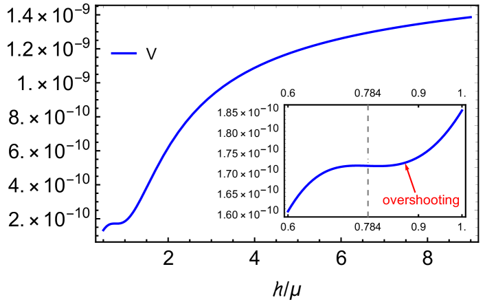
Figure 1: Inflaton potential as function of the variable $x=h/\mu$ for the parameter set (27), which leads to an inflection point at $x=x_{c}=0.784$ leading to an extremely flat region of the potential. Just before this region, there exists an overshooting regime where the universe deviates from the SR expansion since the SR parameters are quite large. Moreover, curvature perturbations are not frozen at super–horizon scales in this regime, as shown in sec. 2.2, making a numerical treatment necessary.

The inflaton potential for these values of the parameters is shown in Fig. 1. It features an inflection point at $x=x_{c}=0.784$. Again following ref. [49], we introduce one more free parameter $\beta$ in order to study slight deviations from a perfect inflection point:

$$a\to a(x_{c},c),\ \ b\to(1-\beta)b(x_{c},c),$$ (28)

where $a(x_{c},c)$ and $b(x_{c},c)$ are the values of the parameters which lead to $V^{\prime}(x_{c})=V^{\prime\prime}(x_{c})=0$. This is of interest since the inflaton field can linger near a true inflection point for a very large number of e–folds. This modification can give a slight slope to the ultra–flat region. Of course, the shape of the overshooting region, in particular $V^{\prime\prime}$, will also be slightly modified: the larger the slope in the ultra–flat region is, the smaller $V^{\prime\prime}$ will be in the overshooting regime. We will use $\beta$ in the range $10^{-5}$ to $10^{-4}$.

3.2 Parameters of the CMB Power Spectrum

The inflaton dynamics in the Einstein frame is given by the Klein–Gordon equation in curved space:

$$\ddot{\chi}+3H\dot{\chi}+\frac{dV}{d\chi}=0\,.$$ (29)

Using the relation between the number of e–folds and time, $dN=Hdt$, we can rewrite eq.(29) as [87, 57]

$$\frac{d^{2}\chi}{dN^{2}}+3\frac{d\chi}{dN}-\frac{1}{2}\left(\frac{d\chi}{dN}\right)^{3}+\left[3-\frac{1}{2}\left(\frac{d\chi}{dN}\right)^{2}\right]\frac{V^{\prime}(\chi)}{V(\chi)}=0\,.$$ (30)

The two Hubble SR parameters are defined as

$$\epsilon_{H}=\frac{1}{2}\frac{\dot{\chi}^{2}}{H^{2}}=\frac{1}{2}\left(\frac{d\chi}{dN}\right)^{2}$$ (31)

and

$$\eta_{H}=-\frac{\ddot{\chi}}{H\dot{\chi}}=\epsilon_{H}-\frac{1}{2\epsilon_{H}}\frac{d\epsilon_{H}}{dN}\,.$$ (32)

SR inflation requires $\epsilon_{H}\ll 1$ and $|\eta_{H}|\ll 1$.

We have seen in sec. 2.2 that under the SR approximation, curvature perturbations are basically frozen at super–horizon scales. The power spectrum is therefore usually computed at horizon crossing, defined by $k=aH$, and can be analytically given by [88] (see appendix A for details):

$$\mathcal{P}_{\zeta}\simeq\frac{H^{2}}{8\pi^{2}\epsilon_{H}}\Bigg{|}_{N=N_{\rm cross}}\,,$$ (33)

where $N_{\rm cross}$ denotes the number of e–folds at horizon crossing. The scale dependence of $\mathcal{P}_{\zeta}$ is usually parameterized as a power law, with spectral index $n_{s}$ given by

$$n_{s}-1=\frac{d\ln\mathcal{P}_{\zeta}}{d\ln k}\simeq-4\epsilon_{H}+2\eta_{H}\,.$$ (34)

The deviation from an exact power law is described by the “running” of the spectral index, parameterized through the quantity $\alpha$:

$$\alpha=\frac{dn_{s}}{d\ln k}\simeq\left(-8\epsilon_{H}^{2}+8\epsilon_{H}\eta_{H}+2\frac{d\eta_{H}}{dN}\right)\,.$$ (35)

The final CMB observable of phenomenological interest is the tensor to scalar ratio $r$, i.e. the perturbations in tensor modes (which can be probed via the polarization of the CMB) normalized to the scalar perturbations. To leading order in SR parameters,

$$r\simeq 16\epsilon_{H}\,.$$ (36)

Now our task is to solve eq.(30), from which the parameters of the CMB power spectrum can be computed. We find it more convenient to calculate the evolution of $x$, rather than the canonically normalized field $\chi$; this is because we have an explicit expression for $V(x)$, see eq.(26), and thus also for $V^{\prime}(x)$. By using eq.(23), eq.(30) and $x=h/\mu$, we find the differential equation for $x$ is:

$$\begin{split}\mu\left[\frac{d^{2}x}{dN^{2}}g(x)+\frac{dx}{dN}\frac{dg(x)}{dN}\right]+3\mu\ g(x)\frac{dx}{dN}-&\frac{1}{2}\left(\mu\,g(x)\frac{dx}{dN}\right)^{3}\\ &+\left[3-\frac{1}{2}\left(\mu\,g(x)\frac{dx}{dN}\right)^{2}\right]\frac{1}{\mu\,g(x)}\frac{V^{\prime}(x)}{V(x)}=0\,.\end{split}$$ (37)

We have renamed $\frac{d\chi}{dh}(x)\equiv g(x)$ for convenience, see eq.(23), with $dg/dN=(dx/dN)dg/dx$. Eq.(37) is too complicated to solve analytically. For a numerical solution we have to choose initial values for $x$ and $dx/dN$ at some $N=N_{0}$. The initial value of $x$ should evidently be above the field values where the CMB scales cross the horizon, so that our solution covers the entire range of scales probed by the CMB and other cosmological observations. On the other hand, it would be wasteful to choose $x(N_{0})$ to be much larger than the field values probed by the CMB, since this earlier evolution leaves no observable traces anyway. In practice we have used $x(0)=8.5$. At these large field values the potential is very flat; if the initial kinetic energy of the field is not very large, the field evolution will therefore quickly approach the SR solution. The initial choice of $dx/dN$ is therefore largely irrelevant; we chose $dx/dN=-0.21$, which corresponds to assuming the SR solution already at $N=N_{0}=0$.

With these initial conditions, eq.(37) can be then solved numerically. Once $x(N)$ is known, the evolution of the canonical field $\chi$ can be obtained by integrating eq.(23):

$$\chi(N)=\int_{0}^{N}\mu\,g(x(N^{\prime}))\,\frac{dx}{dN^{\prime}}\,dN^{\prime}+\chi(0)\,.$$ (38)

The constant of integration $\chi(0)$ can be fixed by using the fact that $g(x)\to 1$ for $x\to 0$; the natural choice is thus $\chi\simeq h$ for $\xi h\ll 1$, which corresponds to $\chi(0)=6.94$.

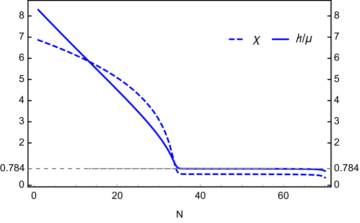
Figure 2: Evolution of the Higgs field with $N$. The universe expands by more than 30 e–folds while the inflaton field traverses the flat region of the potential around the pseudo–critical point $x=x_{c}=0.784$; this corresponds to the USR phase. Between SR and USR, there is an intermediate overshooting stage where the canonically normalized inflaton field $\chi$ varies rather quickly with $N$.

Fig. 2 shows the evolution of $x$ as well as the canonically normalized field $\chi$ with $N$ for our standard set of parameters (27) with $\beta=10^{-5}$. We see that the field at first gradually decreases with increasing $N$; this is the usual SR phase, for large field values. The evolution of $\chi$ becomes quite fast at $N\simeq 30$, signaling a break–down of SR. However, from $N\simeq 36$ both $x$ and $\chi$ remain nearly constant for more than $30$ e–folds; this is when the inflaton traverses the very flat part of the potential around the pseudo–critical point. Evidently the behavior of the field differs qualitatively from that in the SR phase, justifying the use of the expression “ultra–slow roll” for much of this epoch. Inflation ends when the inflaton leaves this region.

Once the dynamics of the inflaton field is known, the parameters of the CMB power spectrum can be computed. Using our standard parameter set (27) and $\beta=10^{-5}$ we find that the CMB “pivot scale” $k=0.05\ \mathrm{Mpc^{-1}}$ crosses out of the horizon at $N_{\rm end}-N_{\rm CMB}\approx 68$. The numerical values of the CMB parameters at this scale are

$$\mathcal{P}_{\zeta}=2.09\times 10^{-9};\ n_{s}=0.951;\ \alpha=-0.0018;\ r=0.043\,,$$ (39)

which is consistent with the Planck 2018 results [89] at the $2\sigma$ level. The large value of $N_{\rm end}-N_{\rm CMB}$ is to a large extent due to the USR phase. This number of e–folds can be reduced by increasing $\beta$, which increases the slope of the potential near the pseudo–critical point. For example, using $\beta=10^{-4}$, we find the same predictions as given by eq.(39) at $N_{\rm end}-N_{\rm CMB}\approx 63$.

3.3 Slow-roll Violation

For our standard set of parameters, CMB scales first crossed out of the horizon during a SR phase, i.e. the SR approximation works very well for the predictions collected in eq.(39). However, Fig. 2 also shows that the canonically normalized inflaton field $\chi$ moves rather fast for $N\simeq 33$. In this subsection we show that the SR conditions are indeed violated in this “overshooting” region.

The dependence of the potential and its first and second derivatives, both with respect to $x$ and with respect to $\chi$, are plotted as function of $N$ in Fig. 3a. The first derivatives remain positive and fairly small throughout. The second derivatives are initially small and negative, but increase in size as the inflaton field approaches the overshooting region, where the second derivative changes very rapidly from large negative to large positive values; in the region around the pseudo–critical point the second derivatives are again very small.

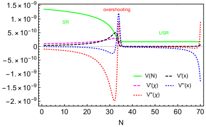
(a)

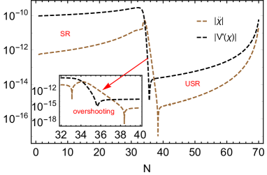
(b)

Figure 3: The left frame shows the evolution of potential and its derivatives with $N$. There is a first SR phase at $N<30$ where all derivatives are small, and a USR phase at $N>38$ where the derivatives are indistinguishable from zero on the shown scale. In between there is an overshooting stage where the curvature of the potential is rather large and varies rapidly; in this regime the SR approximation breaks down and entropic perturbations are excited. This is further illustrated in the right frame which compares the second time derivative $\ddot{\chi}$ of the canonically normalized inflaton field with the slope of the potential; in the overshooting region, $N\sim 35$, the former considerably exceeds the latter in magnitude.

When discussing non–adiabatic pressure perturbations in Sec. 2, we had assumed that the second time derivative of the inflaton field is much larger in magnitude than the slope of the potential. Fig. 3b shows that this is indeed the case for some range of $N$ around $35$. In this case eq.(29) becomes

$$\ddot{\chi}+3H\dot{\chi}\approx 0,$$ (40)

which implies

$$\eta_{H}=-\frac{\ddot{\chi}}{H\dot{\chi}}\approx 3.$$ (41)

In SR, both $\epsilon_{H}$ and $|\eta_{H}|$ should be (much) smaller than $1$; the result (41) clearly violates this.

This is further illustrated in Fig. 4, which shows the evolution of the SR parameters with $N$ for the same set of parameters. We show both the “Hubble” SR parameters defined in eqs.(31) and (32) and their “potential” analogues, defined via

$$\epsilon_{V}=\frac{1}{2}\left(\frac{V^{\prime}}{V}\right)^{2}\,,\ \ \eta_{V}=\frac{V^{\prime\prime}}{V}\,.$$ (42)

SR implies that $\epsilon_{H}\simeq\epsilon_{V}$ and $\eta_{H}\simeq\eta_{V}$; we see that in our case this holds for $N<30$ as well as for $N>38$. $\epsilon_{H}$ and $\epsilon_{V}$ always remain significantly smaller than $1$, but vary rapidly, and differ markedly, in the overshooting region.

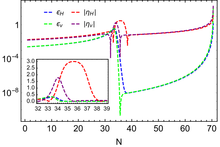
Figure 4: The evolution of the SR parameters with $N$. The parameters defined via the potential almost coincide with those defined via the Hubble parameter in the epochs where the SR approximation holds, but they differ markedly in the overshooting region where $\eta_{H}>1$.

We have shown in sec. 2.2 that entropic perturbation can be excited if the SR conditions are violated, in which case the curvature perturbation are no longer conserved at super horizon scale. Hence the usual estimate (33) of the power spectrum can no longer be justified for modes that first crossed out of the horizon near the overshooting region. In the next section we instead use the Mukhanov–Sasaki (MS) formalism to compute the power spectrum numerically.

3.4 Mukhanov–Sasaki Formalism

Our numerical treatment of the evolution of the curvature perturbations is based on the MS equation; a quick derivation of this equation and its analytical solution in the quasi–de Sitter limit is reviewed in appendix A. It is usually written in terms of the Mukhanov variable

$$v_{k}\equiv-z\zeta_{k}\,,$$ (43)

where $z$ is defined by

$$z^{2}\equiv\left(\frac{d\chi}{dt}\right)^{2}\frac{a^{2}}{H^{2}}=2a^{2}\epsilon_{H}\,.$$ (44)

In these variables, the MS equation reads:

$$\frac{d^{2}v_{k}}{d\tau^{2}}+\left(k^{2}-\frac{1}{z}\frac{d^{2}z}{d\tau^{2}}\right)v_{k}=0,$$ (45)

where $\tau$ denotes the conformal time, i.e. $d\tau=\frac{dt}{a}$.

Rewriting eq.(45) using the number of e–folds $N$ instead of the conformal time gives [57]

$$\begin{split}\frac{d^{2}v_{k}}{dN^{2}}&+(1-\epsilon_{H})\frac{dv_{k}}{dN}\\ &+\left[\frac{k^{2}}{a^{2}H^{2}}+(1+\epsilon_{H}-\eta_{H})(\eta_{H}-2)-\frac{d(\epsilon_{H}-\eta_{H})}{dN}\right]v_{k}=0\,.\end{split}$$ (46)

Under SR conditions the curvature perturbation $\zeta_{k}$ is frozen at super–horizon scales, hence the power spectrum of $\zeta_{k}$ is usually computed at horizon crossing. However, we have seen in the previous subsection that the SR approximation fails in the overshooting regime. In order to account for the evolution of the curvature perturbation also at super–horizon scales the power spectrum should be computed at the end of inflation:

$$\mathcal{P}_{\zeta}(k)=\frac{k^{3}}{2\pi^{2}}\Big{|}\zeta_{k}\Big{|}^{2}_{N=N_{\rm end}}=\frac{k^{3}}{2\pi^{2}}\Big{|}\frac{v_{k}}{z}\Big{|}^{2}_{N=N_{\rm end}}\,.$$ (47)

This can usually only be done numerically. Recall also that super–horizon perturbations are frozen after inflation, as we showed at the very end of Sec. 2.

In order to solve eq.(46), initial conditions are needed. We follow the usual procedure, which assumes the Bunch–Davies vacuum at very early times [90]:

$$\lim\limits_{\tau\to-\infty}v_{k}=\frac{{\rm e}^{-ik\tau}}{\sqrt{2k}}\,.$$ (48)

Since $v_{k}$ is a complex quantity, in practice it is more convenient to solve for its real and imaginary parts separately. To this end one can rewrite the initial condition eq.(48) as [57]:

$$\mathrm{Re}(v_{k})\Big{|}_{N=N_{i}}=\frac{1}{\sqrt{2k}};\ \mathrm{Im}(v_{k})\Big{|}_{N=N_{i}}=0;$$ (49)

$$\mathrm{Re}\left(\frac{dv_{k}}{dN}\right)\Big{|}_{N=N_{i}}=0;\ \mathrm{Im}\left(\frac{dv_{k}}{dN}\right)\Big{|}_{N=N_{i}}=-\frac{\sqrt{k}}{\sqrt{2}a(N_{i})H(N_{i})}\,.$$ (50)

Here $N_{i}$ is the “initial” point where we start the numerical integration of the MS equation. In principle the Bunch–Davis initial conditions (48) should be imposed at $\tau\to-\infty$, which also corresponds to $N\to-\infty$ if the CMB pivot scale crossed the horizon at $N\simeq 0$, as we assumed in the last three figures. Physically this does not make much sense, since we don’t know how many e–folds of inflation happened before that time. Moreover, the ansatz (48) remains a very good approximation of the exact solution of the MS equation as long as the perturbation is well within the horizon, i.e. for $k^{2}\gg a^{2}H^{2}$. Let the mode $k$ cross the horizon at $N=N_{k,{\rm cross}}$. In practice it is then usually sufficient to use $\Delta N\equiv N_{k,{\rm cross}}-N_{i}=2\sim 3$. We have checked that reducing $N_{i}$, which costs a lot of CPU time since the term $k^{2}/(a^{2}H^{2})$ in eq.(46) grows $\propto{\rm e}^{2\Delta N}$ requiring correspondingly reduced step sizes to attain numerical convergence, does not change the final result appreciably. However, we will see below that choosing too small a value for $\Delta N$ can lead to inaccuracies.

3.5 Power Spectrum for Critical Higgs Inflation

We now apply the MS formalism to CHI. In order to compute the power spectrum we have to integrate eq.(46) with the initial conditions eq.(48) till the end of inflation, and then plug the solution into eq.(47).

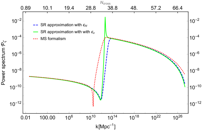
Figure 5: Comparison of the power spectrum computed using the SR approximation (the blue dashed curve corresponds to eq.(33) while the green line represents results with the replacement $\epsilon_{H}\to\epsilon_{V}$) and the MS formalism (red dotted).

The result for our standard parameter set with $\beta=10^{-5}$ is shown in Fig. 5. We see that the SR approximation fails badly for modes crossing the horizon in the vicinity of the overshooting region. In particular, the SR approximation gets both the location and the depth of the dip in the power spectrum wrong by more than one order of magnitude. The approximation (33) using $\epsilon_{H}$ underestimates the maximum of $\mathcal{P}_{\zeta}$ by only a factor of about 1.4, but gets the location $k_{\rm max}$ of the true maximum off by an order of magnitude, and underestimates the power at $k_{\rm max}$ by about five orders of magnitude. Using the approximation (33) but replacing $\epsilon_{H}$ by $\epsilon_{V}$, as is done in much of the older literature on inflation, actually gets $k_{\rm max}$ approximately right, but overestimates the power at this scale by more than two orders of magnitude. In contrast, the SR approximation works well both for the large scales probed by the CMB and for the much smaller scales that cross out of the horizon in the USR regime after the end of the overshooting epoch. The power at these small scales exceeds that at CMB scales by roughly five orders of magnitude due to the overshooting behavior .

In order to better understand the red curve in Fig. 5, in Fig. 6 we show the evolution of $\mathcal{P}_{\zeta}$ with $N$ for four representative values of $k$. These results have been obtained by numerically solving the MS equations; the different curves refer to different values of $N_{i}=N_{\rm cross}-\Delta N$ where the initial conditions (48) have been imposed.

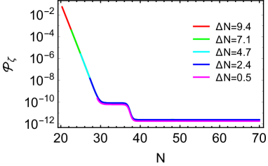
(a) $k=2.5\times 10^{10}\ \mathrm{Mpc^{-1}}$, $N_{\rm cross}=29.7$

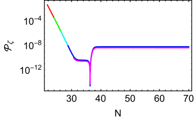
(b) $k=10^{11}\ \mathrm{Mpc^{-1}}$ , $N_{\rm cross}=31.2$

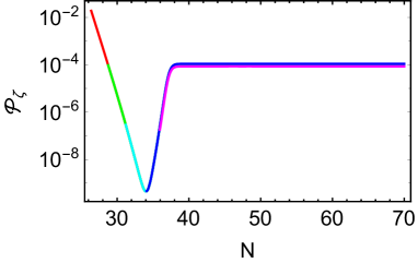
(c) $k=10^{13}\ \mathrm{Mpc^{-1}}$ , $N_{\rm cross}=36.5$

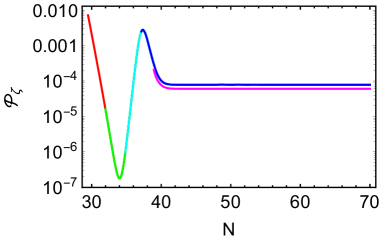
(d) $k=2\times 10^{14}\ \mathrm{Mpc^{-1}}$ , $N_{\rm cross}=39.5$

Figure 6: Evolution of the power spectrum for four different modes which cross the horizon at $N_{\rm cross}$ near the overshooting region. The different colors refer to different initial values $N_{i}=N_{\rm cross}-\Delta N$ when integrating eq.(46). Evidently it is sufficient to use $\Delta N=2\sim 3$ in practice, since the curves for even smaller $N_{i}$ merge with each other, and yield same results. However, using too small $\Delta N$ leads to inaccurate results, for example the one we have showed with $\Delta N=0.5$.

While the results of Fig. 6 have been obtained from eq.(46), the qualitative behavior is more easily understood by combining eqs.(45) and (43), which yields the equivalent differential equation

$$\frac{d^{2}\zeta_{k}}{dN^{2}}+(3+\epsilon_{H}-2\eta_{H})\frac{d\zeta_{k}}{dN}+\frac{k^{2}}{a^{2}H^{2}}\zeta_{k}=0\,.$$ (51)

This equation again has to be satisfied by both the real and imaginary parts of $\zeta_{k}$.

For sub–horizon modes, where $k^{2}\gg a^{2}H^{2}$, the last term in eq.(51) dominates; this by itself leads to an oscillatory behavior of $\zeta_{k}$, with amplitude increasing $\propto{\rm e}^{N/2}$ and with exponentially decreasing oscillation frequency. For SR conditions, $\epsilon_{H},\,|\eta_{H}|\ll 1$, the second term in eq.(51) is a damping term, which reduces the amplitude of the oscillations $\propto{\rm e}^{-3N/2}$. Altogether this yields $\mathcal{P}_{\zeta}\propto{\rm e}^{-2N}$, which explains the initial steep decline in all four cases depicted in Fig. 6.

Of course, the term $\propto k^{2}$ in eq.(51) decreases $\propto{\rm e}^{-2N}$, due to the exponential growth of $a(N)$; by definition the coefficient multiplying $\zeta_{k}$ in this term equals $1$ at $N=N_{\rm cross}$. Moreover, the SR conditions are badly violated in the overshooting region. The evolution of the power depends on where $N_{\rm cross}$ lies relative to the overshooting region. To see this, let us discuss the four cases depicted in Fig. 6 one by one.

Fig. 6a: Here we chose $k=2.5\times 10^{10}\ \mathrm{Mpc^{-1}}$, so that horizon crossing takes place at $N=29.7$, where the SR conditions still hold. As shown in Fig. 6a, the power spectrum for this mode first approaches a constant after horizon crossing. Here the last term in eq.(51) is negligible. As long as the coefficient of the second term is close to $+3$, the absolute value of the first derivative of $\zeta_{k}$ keeps decreasing exponentially with increasing $N$; this corresponds to an overdamped oscillator. The solution for this range of $N$ can thus be written as $\zeta_{k}(N)=C_{1}+C_{2}e^{-3(N-N_{\rm cross})}$, where $C_{1},C_{2}$ are two constants determined by the initial conditions. Let $N_{\rm SR}$ denote the number of e–folds which $\zeta_{k}$ undergoes in the SR regime after horizon crossing, but before overshooting; then this epoch suppresses the first derivative of $\zeta_{k}$ by a factor ${\rm e}^{-3N_{\rm SR}}$. Since the derivative of $\zeta_{k}$ is small, $\zeta_{k}$ itself is basically constant.

This solution is no longer valid in the overshooting region, where $\eta_{H}\approx 3$ while $\epsilon_{H}$ remains rather small, so that $(3+\epsilon_{H}-2\eta_{H})\approx-3$, i.e. the second term in eq.(51) changes sign relative to the SR epoch. This means that now the first derivative to $\zeta_{k}$ begins to grow exponentially in magnitude, however without changing sign. At the end of this epoch one thus has $\zeta_{k}(N)=C_{3}+C_{4}{\rm e}^{+3N_{\rm OS}}$, where $N_{\rm OS}$ is the total “length” of the overshooting epoch, i.e. the number of e–folds during which $\eta_{H}\approx 3$. By matching the two solutions for $\zeta_{k}$ at the point where the overshooting epoch begins, one finds $C_{1}=C_{3}$ and $C_{4}=-C_{2}{\rm e}^{-3N_{\rm SR}}$. So after overshooting ends, the value of $\zeta_{k}$ is approximately given by $\zeta_{k}=C_{1}-C_{2}e^{3\left(N_{\rm OS}-N_{\rm SR}\right)}$. Since afterwards the SR conditions hold again, $\zeta_{k}$ remains approximately constant, i.e. this result still holds at the end of inflation.

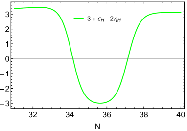
(a) Evolution of $A$.

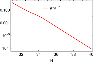
(b) Evolution of $B$.

Figure 7: Evolution of the two coefficients in eq.(51); the left frame is independent of $k$, while the result of the right holds for $k=10^{11}\ \mathrm{Mpc^{-1}}$ and scales $\propto k^{2}$.

The overshooting region will therefore only have significant impact on the final power for modes that crossed out of the horizon not much more than $N_{\rm OS}$ e–folds before its onset. From the left frame of Fig. 7 we read off that for our numerical example overshooting starts at $N\approx 34$, with $N_{\rm OS}\approx 3.5$. For the case considered in Fig. 6a $N_{\rm OS}$ and $N_{\rm SR}$ are comparable. For much smaller co–moving wave number $k$, $N_{\rm SR}\gg N_{\rm OS}$, so that the effect of the overshooting region on the final power is not significant. This explains why the standard SR approximation works for $k<10^{10}\ \mathrm{Mpc^{-1}}$ in Fig. 5.

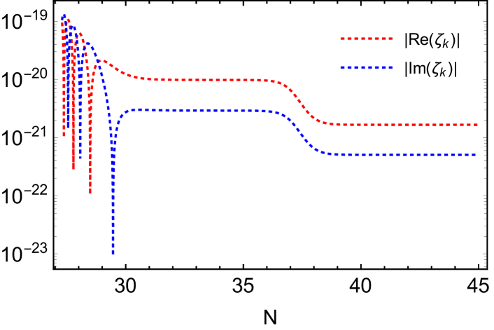
Figure 8: Evolution of curvature perturbations for the mode with co–moving $k=2.5\times 10^{10}\ \mathrm{Mpc^{-1}}$. This figure shows the epoch from a few e–folds before horizon crossing to a few e–folds after the end of the overshooting region.

The detailed evolution of the real and imaginary parts of $\zeta_{k}$ is shown in Fig. 8. Note that the overshooting region has significant impact on $\zeta_{k}$ itself (as opposed to its derivative) only beginning at $N\approx 37$, where the exponential growth of the modulus of the derivative compensated its exponential suppression between horizon crossing and the onset of the overshooting epoch. Since overshooting already ends at $N\approx 38$, its total effect is still moderate for this value of $k$. Notice, however, that the second flat region lies well below the first one, which corresponds to the prediction of the usual analytical SR estimates. This is because in the overdamped oscillator phase just after horizon crossing, the first derivative of $\zeta_{k}$ always has the opposite sign as $\zeta_{k}$ itself, for both the real and imaginary part. The exponential decrease of the modulus of the derivatives will therefore decrease $|\zeta_{k}|$, and thus $\mathcal{P}_{\zeta}$. We will come back to this point shortly.

Fig. 6b: for co–moving $k=10^{11}\ \mathrm{Mpc^{-1}}$, $\mathcal{P}_{\zeta}$ nearly vanishes for a value of $N$ during the overshooting epoch. Now the nominal horizon crossing at $N=31.2$ occurs just before the onset of the overshooting epoch, which means we cannot always assume $k\ll aH$ when we discuss the evolution of the curvature perturbation around the overshooting regime. In the following discussion we denote the coefficient of the second and third terms in eq.(51) by $A$ and $B$, respectively; their dependence on $N$ is depicted in Fig. 7. After horizon crossing, the evolution of $\zeta_{k}$ undergoes four stages, which are shown in Fig. 9:

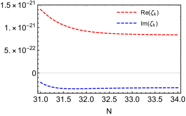
(a) $31<N<34$

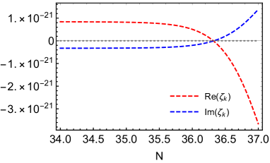
(b) $34<N<37$

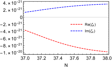
(c) $37<N<38$

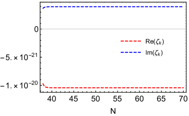
(d) $38<N<70$

Figure 9: Evolution of curvature perturbations for the mode with co–moving wave number $k=10^{11}\ \mathrm{Mpc^{-1}}$.

• $31<N<34$, Fig. 9a: in this region, $A$ is always positive and therefore acts as a friction term, and $B$ decreases exponentially. Since we are already beyond horizon crossing, $B^{2}-A^{2}/4<0$, i.e. eq.(51) approximately describes an over–damped oscillator. This means that $\zeta_{k}$ does not oscillate any more, but decreases rather slowly. This explains the first, short flat region in Fig. 6b. In this region the second derivative of $\zeta_{k}$ can be neglected, thus the curvature perturbation satisfies $\frac{d\zeta_{k}}{dN}\approx\frac{B}{A}\zeta_{k}$. This approximation ceases to hold somewhat before the value $N_{0}$ where $A$ turns to zero, i.e. where the overshooting region starts; recall that in our case $N_{0}\approx 34$.

• $34<N<37$, Fig. 9b: for $N\geq N_{0}$, $B\leq 0.01$ (see Fig. 7) has become essentially negligible, while $A$ changes from positive to negative hence acts as a driving term. As discussed above this leads to an exponential increase of the first derivative of $\zeta_{k}$. Since the epoch of exponentially decreasing first derivatives is considerably shorter than for $k=2.5\cdot 10^{10}\ \mathrm{Mpc^{-1}}$, $\zeta_{k}$ itself now begins to vary appreciably already at $N\approx 36$.

  Remarkably, shortly thereafter both the real and imaginary parts cross the zero point nearly at the same time, leading to $\zeta_{k}\to 0$. This can be understood from the approximate solution for $\zeta_{k}$ in this range of $N$:

  $$\zeta_{k}(N)\approx\zeta_{k}(N_{0})-\frac{1}{A}\frac{d\zeta_{k}}{dN}\Big{|}_{N_{0}}\left({\rm e}^{-A(N-N_{0})}-1\right).$$ (52)

  Since $\frac{d\zeta_{k}}{dN}\Big{|}_{N_{0}}\propto\zeta_{k}(N_{0})$, we see that the real and imaginary parts of $\zeta_{k}(N)$ go through zero at the same point, which is also the origin of the very sharp minimum depicted in Fig. 6b. Note that for the previous case, $k=2.5\cdot 10^{10}\ \mathrm{Mpc^{-1}}$, the overshooting epoch ended before $\zeta_{k}$ reached zero; the sharp minimum of the final power spectrum depicted in Fig. 5 corresponds to that value of $k$ where the overshooting epoch lasts just long enough to drive $\zeta_{k}$ to zero, and then ends. In the case at hand instead $|\zeta_{k}|$ again increases exponentially beyond the zero crossing.

• $37<N<38$, Fig. 9c: this is the stage just after the overshooting epoch, i.e. $A$ is again positive so that the modulus of the first derivative of $\zeta_{k}$ is decreasing exponentially again. For a while $|\zeta_{k}|$ keeps increasing, albeit more slowly than before. Of course, $B\leq 10^{-5}$ is now completely negligible.

• $38<N<70$, Fig. 9d: the overshooting phase has ended and the universe comes back to (U)SR inflation, therefore curvature perturbations are frozen again at the super horizon scale and matter perturbation evolve adiabatically again. This corresponds the second flat region shown in Fig. 6b. For this value of $k$ the second flat region is already higher than the first one, thus the analytical SR approximation underestimates the final power.

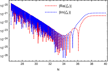
(a)

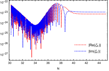
(b)

Figure 10: Evolution of curvature perturbations for the modes with co–moving wave number $k=10^{13}\ \mathrm{Mpc^{-1}}$ (left) and $k=2\times 10^{14}\ \mathrm{Mpc^{-1}}$ (right).

Fig. 6c: for the mode with $k=10^{13}~{}\mathrm{Mpc^{-1}}$, horizon crossing occurs at $N=36.5$; this lies in the middle of the overshooting regime. Hence there is no overdamped oscillator phase, and therefore also no plateau in the evolution of $\mathcal{P}_{\zeta}$, before the overshooting epoch, unlike in Figs. 6a and 6b.

Nevertheless for $N<34$ eq.(51) again describes a damped oscillator, the amplitude of the oscillation decreasing $\propto{\rm e}^{-N}$. This is also shown in Fig. 10a. However, at $N=N_{0}\simeq 34$ the second term in eq.(51) changes sign, eventually reaching $-3$ as shown in Fig. 7. For $N_{0}<N<N_{\rm cross}$ eq.(51) therefore leads to oscillations whose amplitude grows $\propto{\rm e}^{2N}$. For $N>N_{\rm cross}$ the approximately exponential growth continues for a while, this time for $|\zeta_{k}|$ itself which no longer oscillates. As before, for $N>37$ the derivative of $\zeta_{k}$ begins to decrease exponentially in magnitude, which leads to $\zeta_{k}$ itself becoming essentially constant for $N>38$, after the end of the overshooting epoch. Not surprisingly, for this mode the analytical SR estimate for the final power also fails.

Fig. 6d: for the mode with co–moving wave number $k=2\times 10^{14}~{}\mathrm{Mpc^{-1}}$, horizon crossing takes place at $N=39.5$, i.e. during USR well after the end of the overshooting epoch. We again see an (initially very rapid) oscillation whose amplitude first drops $\propto{\rm e}^{-N}$ and then increases $\propto{\rm e}^{2N}$ once $N>34$, i.e. in the overshooting regime. Since for this value of $k$ the overshooting epoch ends before horizon crossing, for $N>38$ the function $\zeta_{k}$ again undergoes a few oscillations with exponentially decreasing amplitude, before settling into an overdamped oscillator mode, i.e. approaching a constant.

In this case the analytical SR approximation for the final power actually works quite well. On the one hand this may not be surprising, since the arguments of Sec. 2 imply that perturbations are now adiabatic at super–horizon scales. On the other hand, it may be surprising that one still gets the correct result by imposing the initial conditions (48) just a couple of e–folds before horizon crossing. This implies that these initial conditions capture the dynamics of the MS equation even in the overshooting regime, as long as the mode is still (deep) inside the horizon.

In fact, eq.(48) shows that $|v_{k}|$ is simply a constant (independent of $N$) for sub–horizon modes. The dynamics is therefore entirely captured by the factor $1/z$ which relates $\zeta_{k}$ to $v_{k}$, see eq.(44). This contains a factor $1/a\propto{\rm e}^{-N}$, which dominates the $N-$dependence in the (U)SR regime where the SR parameter $\epsilon_{H}$ is approximately constant (and small). However, eq.(30) shows that in the overshooting regime, where the term containing the derivative of the potential can be neglected, $\sqrt{\epsilon_{H}}\propto|d\chi/dN|\propto{\rm e}^{-3N}$, so that altogether $|\zeta_{k}|\propto 1/(a\sqrt{\epsilon_{H}})\propto{\rm e}^{+2N}$, as we had inferred from the MS equation.

For modes with even larger $k$, the situation is very similar to the case with $k=2\times 10^{14}~{}\mathrm{Mpc^{-1}}$, i.e. the analytical SR approximation for the final power agrees with the numerical result, as shown in Fig. 5, as long as the modes cross out of the horizon (well) before the end of inflation. The approximation fails again for modes with very large $k$ which cross the horizon near the end of inflation where SR again fails; however, we know of no way to probe those modes observationally.

From the above discussion it is easy to understand that the peak in the power spectrum shown in Fig. 5 occurs for the mode which crosses the horizon just at the beginning of the overshooting regime. In this case, $N_{\rm SR}=0$, and the exponential increase of $|d\zeta_{k}/dN|$ is maximized. This also greatly enhances the final value of $|\zeta_{k}|$, leading to the maximum in the spectrum. We find the maximal scalar power spectrum is $\mathcal{P}_{\zeta}\approx 1.1\times 10^{-4}$ for $k=1.1\cdot 10^{13}\mathrm{Mpc^{-1}}$. According to ref. [49], fluctuations of this size are large enough to lead to significant formation of primordial black holes, which might even constitute a sizable fraction of all dark matter. In the next section we will investigate another cosmological consequence of such a large curvature perturbation, namely the amplification of primordial gravitational wave signatures due to second order effects.

Before closing this section we comment on possibilities to increase the power spectrum even further. According to ref. [63], quantum diffusion effects can in principle further enhance the power; however, we checked that in our case one always has $|\dot{\chi}|\gg H^{2}/(2\pi)$, which indicates that quantum diffusion does not change the evolution of the inflaton field significantly. Moreover, refs. [57, 97] argue that a shallow local minimum of the inflaton potential can also enhance the power spectrum; this agrees with our finding in eq.(18), because the curvature of the potential $V^{\prime\prime}$ is maximal near a local minimum. However, the inflaton might get stuck in a local minimum, in which case inflation would never end. In contrast, the scenario we presented leads to a well–behaved inflationary epoch, in agreement with current observations.

4 Second Order Gravitational Wave Signatures

As well known, primordial perturbations of the inflaton field source primordial gravitation waves. Usually the strength of the GW signal is estimated in linear order in perturbations; for SR inflation, this leads to the famous prediction $r=16\epsilon_{V}$, where $r$ is the tensor–to–scalar ratio. However, in some cases effects that are second order in the curvature perturbations can also contribute significantly to the primordial GW signal [98, 99, 100, 101]. As has recently been emphasized in [51], which analyses a polynomial potential with an inflection point, this occurs in particular when an overshooting regime enhances the power spectrum. In the following analysis, we mainly follow the formalism given in [100, 51].

In the radiation era, the second order tensor perturbation with comoving wave number $k$ satisfies [107, 100, 102, 103, 104, 105, 106, 51]:

$$h^{\prime\prime}(\vec{k},\tau)+2aHh^{\prime}(\vec{k},\tau)+k^{2}h(\vec{k},\tau)=S(\vec{k},\tau)\,,$$ (53)

where a prime denotes a derivative with respect to the conformal time $\tau$. $S(\vec{k},\tau)$ denotes the source term, which is given by [51]

$$\begin{split}S(\vec{k},\tau)=\int\frac{d^{3}\tilde{k}}{(2\pi)^{3/2}}\tilde{k}^{2}\Bigg{[}1&-\Bigg{(}\frac{\vec{k}\cdot\vec{\tilde{k}}}{k\tilde{k}}\Bigg{)}^{2}\Bigg{]}\Bigg{[}12\Phi(\vec{k}-\vec{\tilde{k}},\tau)\Phi(\vec{\tilde{k}},\tau)\\ &+8\Bigg{(}\tau\Phi(\vec{k}-\vec{\tilde{k}},\tau)+\frac{\tau^{2}}{2}\frac{d\Phi(\vec{k}-\vec{\tilde{k}},\tau)}{d\tau}\Bigg{)}\frac{d\Phi(\vec{\tilde{k}},\tau)}{d\tau}\Bigg{]}\,.\end{split}$$ (54)

The Bardeen potential appearing in eq.(54) is related to the curvature perturbation via $\Phi=2\zeta_{k}/3$ [51]. As we have seen in the last section, the scalar curvature perturbation is enhanced during an overshooting regime, thus we expect that the source term for gravitational waves will also be enhanced.

In order to obtain the current gravitational wave density, we have to solve eq.(53) with source given by eq.(54). To that end we’ll apply the Green’s function method of ref. [100]. Rewriting eq.(53) with $v:=ah$, we get

$$v^{\prime\prime}(\vec{k},\tau)+\left(k^{2}-\frac{a^{\prime\prime}}{a}\right)v(\vec{k},\tau)=aS(\vec{k},\tau)\,.$$ (55)

The solution of eq.(53) can then be written as

$$h(\vec{k},\tau)=\frac{1}{a(\tau)}\int d\tilde{\tau}g(\vec{k},\tau;\tilde{\tau})\left[a(\tilde{\tau})S(\vec{k},\tau)\right]\,,$$ (56)

where $g$ is the Green’s function for eq.(55), which satisfies:

$$g^{\prime\prime}(\vec{k},\tau;\tilde{\tau})+\left(k^{2}-\frac{a^{\prime\prime}}{a}\right)g(\vec{k},\tau;\tilde{\tau})=\delta(\tau-\tilde{\tau})\,.$$ (57)

Once the tensor perturbations are known, we can further compute the contribution of these primordial gravitational waves to the total energy budget of the universe. For a matter-dominated universe, one has [100]:

$$\Omega^{(2)}_{\rm GW}(k,\tau)=A^{(2)}_{\rm GW}\mathcal{P}^{2}_{\zeta}\cdot\begin{cases}\frac{a(\tau)}{a_{\rm eq}}\frac{k}{k_{\rm eq}}&\text{if}\ k<k_{\rm eq}\\ \frac{a(\tau)}{a_{\rm eq}}\left(\frac{k}{k_{\rm eq}}\right)^{2-2\gamma}&\text{if}\ k_{\rm eq}<k<k_{c}(\tau)\\ \frac{a_{\rm eq}}{a(\tau)}&\text{if}\ k>k_{c}(\tau)\\ \end{cases}\,.$$ (58)

Here $k_{c}(\tau)=\left(\frac{a(\tau)}{a_{\rm eq}}\right)^{1/(\gamma-1)}k_{\rm eq}$, $A^{(2)}_{\rm GW}\simeq 10$, and $\gamma\simeq 3$ [100]. Finally, $k_{\rm eq}\approx 0.01\mathrm{Mpc^{-1}}$ [108] denotes the wave number that re–entered the horizon when matter and radiation had the same energy density and $a_{\rm eq}\equiv 1/(1+z_{\rm eq})$ denotes the scale factor at that time. Eqs.(58) hold after matter–radiation equilibrium, i.e. for $\tau>\tau_{\rm eq}$ where $k_{c}(\tau)>k_{\rm eq}$. We are interested in the gravitational wave signatures in the range of wave numbers that are enhanced by the scalar perturbation in the overshooting regime, $10^{11}\mathrm{Mpc^{-1}}<k<10^{14}\mathrm{Mpc^{-1}}$ (see Fig. 5). These are much larger than $k_{c}(\tau_{0})$; the present ($\tau=\tau_{0}$ with $a(\tau_{0})=1$) GW signal is thus [100, 51]

$$\Omega^{(2)}_{\rm GW}(k,\tau_{0})\simeq 10\ \mathcal{P}^{2}_{\zeta}\ a_{\rm eq}\,.$$ (59)

Using $z_{eq}=3387$, $H_{0}=67.4\ \mathrm{km\ s^{-1}Mpc^{-1}}$ [108] and the power spectrum $\mathcal{P}_{\zeta}$ computed via the MS formalism in the last section, we can calculate the current gravitational wave energy density due to this second order effect.

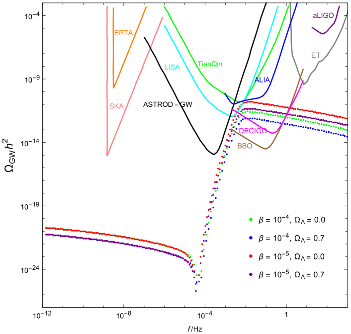
Figure 11: The gravitational wave signal from CHI induced by second order effects, $\Omega_{\rm GW}\propto\mathcal{P}_{\zeta}^{2}$. In the above plot, $f=\frac{ck}{2\pi}$ is the frequency of the gravitational wave, with $c$ the speed of light. The frequency range we have shown is $10^{-12}~{}\mathrm{Hz}<f<10^{3}~{}\mathrm{Hz}$, which corresponds to $10^{3}~{}\mathrm{Mpc^{-1}}<k<6.5\times 10^{17}~{}\mathrm{Mpc^{-1}}$. The experimental sensitivity curves we show include the Square Kilometer Array (SKA), Einstein Telescope (ET), Astrodynamical Space Test of Relativity using Optical-GW detector (ASTROD-GW), Advanced LIGO (aLIGO), European Pulsar Timing Array (EPTA), Laser Interferometer Space Antenna (LISA) [109], Advanced Laser Interferometer Antenna (ALIA), Big Bang Observer (BBO), Deci-hertz Interferometer GW Observatory (DECIGO) and TianQin [110]. The sensitivities of EPTA, SKA, LISA, TianQin and aLIGO limit are taken from [51]. The ALIA, DECIGO, and BBO sensitivity curves are reproduced from [111]. The ASTROD-GW and ET curves are adapted from [112].

The result is shown in Fig. 11, which also shows the sensitivity of several planned gravitational wave detectors. We saw at the end of the last Section that the maximum of the power spectrum is at $k=1.1\times 10^{13}\mathrm{Mpc^{-1}}$, which corresponds to frequency $f=0.017$ Hz. This is near the frequency of maximal sensitivity of the upcoming space mission LISA, which may just barely be able to detect this signal if the parameter $\beta=10^{-5}$ (red curve), while for $\beta=10^{-4}$ (green) the signal is below the foreseen LISA sensitivity. Recall that the CMB predictions for both values of $\beta$ are consistent with latest Planck measurements, see Sec. 3.2. Since a larger $\beta$ makes the potential less flat in the USR region and reduces $V^{\prime\prime}$ in the overshooting region, it is expected that the corresponding curvature perturbation is less enhanced compared to that with a smaller $\beta$ according to eq.(18). This explains why the peak of GW signatures with $\beta=10^{-4}$ is lower. However, the second generation space missions DECIGO and BBO should easily detect this signal even for $\beta=10^{-4}$.

As already noted, eqs.(58) hold for a matter-dominated universe, i.e. for $\tau>\tau_{\rm eq}$ where $k_{c}(\tau)>k_{\rm eq}$. We are not aware of a calculation of $\Omega_{\rm GW}^{(2)}$ that includes dynamical effects due to a cosmological constant; this would be required for very large wavelengths, which crossed the horizon after the cosmological constant (or, more generally, dark energy) contributed significantly to the total energy density. Fortunately we are interested in much shorter wavelengths, with $10^{11}$ Mpc${}^{-1}<k<10^{14}$ Mpc^-1, which crossed the horizon when the cosmological constant was entirely negligible. The further dilution of the gravitation wave signal by the recent accelerated expansion of the universe can then simply be described by multiplying the right-hand side of eqs.(58) with the normalized matter density $\Omega_{m}(\tau)$, yielding a suppression by a factor $\simeq 0.3$ today. These results are shown by the purple and blue lines respectively for $\beta=10^{-5}$ and $\beta=10^{-4}$.

Fig. 11 also shows that the peak of the CHI signal lies at frequencies that are too large for the pulsar timing arrays even after SKA comes on–line. The size of the signal is well below the sensitivity of advanced LIGO, and even below that of the planned Einstein Telescope (ET).

5 Summary and Conclusions

In this paper, we have revisited critical Higgs inflation, carefully computing the power spectrum as well as the gravitational wave signatures induced by second order effects.

In Sec. 2 we analyzed the evolution of curvature perturbations under (ultra–)slow roll as well as overshooting conditions in general terms. In the former, the second derivative of the inflaton field with respect to time can be neglected in the equation of motion; we showed that the perturbations are adiabatic in this case, which further implies that the curvature perturbations are frozen at super–horizon scales. This allows one to calculate the final power spectrum (at the end of inflation), which seeds all observed structures in the universe, by simply computing the power spectrum at horizon crossing. We emphasize that this also holds for ultra–slow roll (USR), which in our model describes the epoch when the inflaton field is near the (almost) saddle point of the potential. Here the deviations from adiabacity are even smaller than in the SR case, so that the usual approximate treatment is even more accurate.

In contrast, when the inflaton enters an overshooting phase where the acceleration $|\ddot{\chi}|$ is much larger than the derivative of the potential $|V^{\prime}|$, we showed that perturbations are no longer adiabatic; this can be described in terms of entropic pressure perturbations. In this case the curvature perturbations are not conserved at super–horizon scales, so that the standard SR approximation for calculating the power spectrum is expected to break down. To our knowledge this is the first time that the significance of entropic perturbations has been discussed in this context. Our eq.(18) shows that the enhancement of the perturbations after horizon crossing but during the overshooting epoch will increase for larger curvature $V^{\prime\prime}$ of the potential. This can be very useful for inflationary model building if one wants to strongly enhance the power spectrum, e.g. in order to produce primordial black holes. See [113] for a recent investigation along this direction.

In Sec. 3 we illustrated these general results by analyzing the CHI scenario in detail. For judiciously chosen parameters, an overshooting epoch appears between the SR and USR eras. During the overshooting stage the Hubble SR parameters vary rapidly, which implies the universe deviates significantly from SR evolution. As a result the usual analytical approximation to compute the power spectrum fails. We instead solved the Mukhanov–Sasaki equation numerically to compute the power spectrum at the end of inflation. We find that the modes which cross the horizon just before or during the overshooting epoch are greatly enhanced. The power spectrum can reach values of order $\sim 10^{-4}$ for $k\sim 10^{13}\ \mathrm{Mpc^{-1}}$; this is to be compared to values of order $10^{-9}$ at the (much smaller) $k-$values probed by the CMB anisotropies. These results differ quantitatively from those of ref.[49], where the power spectrum was computed in the SR approximation.

In the course of this discussion we found a version of the MS equation very useful which holds for the $k-$space perturbation $\zeta_{k}$ directly, rather than for the related quantity $v_{k}$ which is usually employed, see eq.(51). This allowed us to understand the numerical results in detail: why the SR approximation agrees with the MS formalism for modes that cross out of the horizon well before (small $k$) or well after (large $k$) the overshooting epoch; why there is a sharp minimum in the power spectrum, for scales that cross the horizon a few e–folds before the overshooting region; and where the maximum of the spectrum lies. These findings are generic and can also be applied to explain the numerical power spectrum results for other inflation models featuring a near–inflection point, for example [51, 63, 59], where detailed explanations concerning the numerical results are not given.

Finally we analyzed the second order GW signatures induced by the enhanced scalar perturbations. The strength of this signal is proportional to the square of the scalar power spectrum. The peak of the latter at co–moving wave number of order $10^{13}\ \mathrm{Mpc^{-1}}$ corresponds to a peak of the GW signal at a frequency of $0.017$ Hz. We find that for our choices of parameters, the GW signal should remain detectable up to frequency of order $1$ Hz by two planned second–generation space based GW experiments, DECIGO and BBO. Detection of this signal is a firm prediction, if the power spectrum is enhanced to the level that might allow significant production of PBHs. This statement holds also in other models of inflation proposed recently [50, 52, 53, 54, 58, 55, 57, 51, 56, 59]. Hence if future GW experiments fail to detect this signal, one could conclude that no significant PBH formation occurred immediately after inflation.

In this paper we did not consider effects due to non–Gaussianity. Since PBHs only form in regions with large overdensity, their formation rate can be greatly enhanced if there are significant non–Gaussian tails in the distribution function of the density perturbations [114, 115]. It should be noted that the calculation of the PBH formation rate is in any case somewhat uncertain; however, the second order GW signal computed in the Gaussian approximation should be detectable by second generation space missions for the entire range of perturbations that could plausibly lead to sizable PBH formation, unless non–Gaussianities are quite large for the relevant modes. In this context it is important to note that according to a recent analysis [116, 117] primordial non–Gaussianities will also enhance the second order GW signal itself. We leave a detailed investigation of the impact on non–Gaussianities on CHI inflation for future work.

Appendix A Mukhanov-Sasaki Equation and Its Analytical Solution

In this Appendix we briefly review the derivation of the MS equation and discuss its analytical solution in (quasi) de Sitter spacetime.

A.1 Derivation of the Mukhanov-Sasaki Equation

We start from the general action of a single real scalar field minimally coupled to gravity,

$$S=\frac{1}{2}\int d^{4}x\sqrt{-g}\left[R-g^{\mu\nu}\triangledown_{\mu}\phi\triangledown_{\nu}\phi-2V(\phi)\right]\,.$$ (60)

Using the Arnowitt–Deser–Misner (ADM) formalism [118] this action can be expanded as: $S=S_{(0)}+S_{(1)}+S_{(2)}+\dots$, where the order is with respect to the perturbation $\zeta$. $S_{(0)}$ denotes the background, $S_{(1)}$ vanishes due to the first order Hamiltonian constraint equation [121, 119, 120], $S_{(2)}$ contains the two–point correlation function we wish to compute, and higher orders contribute to non–Gaussian contributions to the power spectrum which are beyond the scope of our analysis. In [121, 120], it is shown that the action up to the second order of $\zeta$ can be written as

$$S_{(2)}=\frac{1}{2}\int d^{4}xa^{3}\frac{\dot{\phi}^{2}}{H^{2}}\left[\dot{\zeta}^{2}-a^{-2}(\partial_{i}\zeta)^{2}\right]\,;$$ (61)

here $a$ is the scale factor in the FRW metric. Now define the Mukhanov variable as

$$v\equiv-z\zeta\,,$$ (62)

where $z$ carries the information about the background field:

$$z^{2}\equiv a^{2}\frac{\dot{\phi}^{2}}{H^{2}}=2a^{2}\epsilon_{H}\,.$$ (63)

Transforming the cosmic time $t$ to the conformal time $\tau$ with $d\tau=dt/a$, we can rewrite the action eq.(61) as

$$\begin{split}S_{(2)}&=\frac{1}{2}\int d\tau d^{3}x\left[(v^{\prime})^{2}-(\partial_{i}v)^{2}+\frac{z^{\prime\prime}}{z}v^{2}\right]\\ &=\frac{1}{2}\int d\tau d^{3}x\mathcal{L}_{(2)}\,.\end{split}$$ (64)

Here a prime denotes a derivative with respect to $\tau$. The Euler–Lagrange equation derived from $\mathcal{L}_{(2)}$ reads

$$\frac{\partial\mathcal{L}_{(2)}}{\partial v}-\frac{\partial}{\partial\tau}\left(\frac{\partial\mathcal{L}_{(2)}}{\partial v^{\prime}}\right)-\frac{\partial}{\partial x^{i}}\left(\frac{\partial\mathcal{L}_{(2)}}{\partial_{i}v}\right)=0\,.$$ (65)

Plugging $\mathcal{L}_{(2)}$ from eq.(64) into eq.(65), we obtain:

$$v\frac{z^{\prime\prime}}{z}-v^{\prime\prime}+\partial^{i}\partial_{i}v=0.$$ (66)

It is usually more convenient to analyse the perturbations in Fourier space. To that end we write the field $v$ as:

$$v(\tau,\bm{x})=\int\frac{d^{3}k}{(2\pi)^{3}}\left[v_{\bm{k}}(\tau){\rm e}^{i\bm{k}\cdot\bm{x}}+v^{*}_{\bm{k}}(\tau){\rm e}^{-i\bm{k}\cdot\bm{x}}\right]\,.$$ (67)

Note that $v$ is real by construction, whereas $v_{\bm{k}}$ is usually complex. Moreover, $\bm{k}$ is defined in co–moving coordinates, i.e. it remains unchanged by the expansion of the universe.

The MS equation in $\bm{k}-$space can be found by plugging eq.(67) into eq.(66) [122, 123, 124]:

$$v_{\bm{k}}^{\prime\prime}+\left(k^{2}-\frac{z^{\prime\prime}}{z}\right)v_{\bm{k}}=0\,.$$ (68)

This equation describes how some perturbation with wave vector $\bm{k}$ evolves with time. This equation has no general analytical solution, due to the dependence on the background field dynamics via $z^{\prime\prime}/z$. However, in some special cases, such as the SR inflationary phase, an analytical solution exists, as we explain below.

A.2 Quantization, Initial Condition and Bunch-Davies Vacuum

Before discussing analytical solutions of eq.(68) we first describe the quantization of our field. After all, the physical origin of the curvature perturbations generated by inflation are quantum fluctuations of the inflaton field. Using the canonical quantization procedure, we write the QFT analogue of the classical Fourier decomposition of eq.(67) [81]:

$$\hat{v}=\int\frac{d^{3}k}{(2\pi)^{3}}\left[v_{\bm{k}}(\tau)\hat{a}_{\bm{k}}{\rm e}^{i\bm{k}\cdot\bm{x}}+v^{*}_{\bm{k}}(\tau)\hat{a}^{\dagger}_{\bm{k}}{\rm e}^{-i\bm{k}\cdot\bm{x}}\right]\,,$$ (69)

where $\hat{a}_{\bm{k}}$ and $\hat{a}^{\dagger}_{\bm{k}}$ are annihilation and creation operators. The corresponding Fourier modes corresponding to a fixed co–moving wave vector $\bm{k}$ are

$$\hat{v}_{\bm{k}}=v_{\bm{k}}(\tau)\hat{a}_{\bm{k}}+v^{*}_{-\bm{k}}(\tau)\hat{a}^{\dagger}_{-\bm{k}}\,;$$ (70)

note that $v_{\bm{k}}$ in eqs.(69) and (70) again satisfy the (classical) MS equation (68).

Similarly one can also introduce the quantum version of the canonical momentum variable $\pi=\frac{\partial{\cal L}_{2}}{\partial v^{\prime}}=v^{\prime}$:

$$\hat{\pi}=\int\frac{d^{3}k}{(2\pi)^{3}}\left[v_{\bm{k}}^{\prime}(\tau)\hat{a}_{\bm{k}}{\rm e}^{i\bm{k}\cdot\bm{x}}+v^{*\prime}_{\bm{k}}(\tau)\hat{a}^{\dagger}_{\bm{k}}{\rm e}^{-i\bm{k}\cdot\bm{x}}\right]\,.$$ (71)

We impose the canonical commutation relation between $\hat{v}$ and its conjugate momentum variable $\hat{\pi}$,

$$[\hat{v}(\tau,\bm{x}),\,\hat{\pi}(\tau,\bm{y})]=i\delta(\bm{x}-\bm{y})\,.$$ (72)

From eqs.(69) and (71) we see that this requires

$$\begin{split}i\delta(\bm{x}-\bm{y})&=\int\frac{d^{3}k}{(2\pi)^{3}}\frac{d^{3}q}{(2\pi)^{3}}\Big{[}v_{\bm{k}}v_{\bm{q}}^{\prime}\left(\hat{a}_{\bm{k}}\hat{a}_{\bm{q}}-\hat{a}_{\bm{q}}\hat{a}_{\bm{k}}\right){\rm e}^{i(\bm{k}\cdot\bm{x}+\bm{q}\cdot\bm{y})}+v_{\bm{k}}v_{\bm{q}}^{\star\prime}\left(\hat{a}_{\bm{k}}\hat{a}_{\bm{q}}^{\dagger}-\hat{a}^{\dagger}_{\bm{q}}\hat{a}_{\bm{k}}\right){\rm e}^{i(\bm{k}\cdot\bm{x}-\bm{q}\cdot\bm{y})}\\ &+v_{\bm{k}}^{\star}v_{\bm{q}}^{\prime}\left(\hat{a}^{\dagger}_{\bm{k}}\hat{a}_{\bm{q}}-\hat{a}_{\bm{q}}\hat{a}^{\dagger}_{\bm{k}}\right){\rm e}^{i(\bm{q}\cdot\bm{y}-\bm{k}\cdot\bm{x})}+v_{\bm{k}}^{\star\prime}v_{\bm{q}}^{\star\prime}\left(\hat{a}^{\dagger}_{\bm{k}}\hat{a}^{\dagger}_{\bm{q}}-\hat{a}^{\dagger}_{\bm{q}}\hat{a}^{\dagger}_{\bm{k}}\right){\rm e}^{-i(\bm{k}\cdot\bm{x}+\bm{q}\cdot\bm{y})}\Big{]}\,.\end{split}$$ (73)

Eq.(73) implies

$$-i(v_{\bm{k}}v^{*\prime}_{\bm{q}}-v^{\prime}_{\bm{k}}v^{*}_{\bf{q}})[\hat{a}_{\bm{k}},\hat{a}^{\dagger}_{\bm{q}}]=(2\pi)^{3}\delta(\bm{k}-\bm{q})\,;$$ (74)

$$v_{\bm{k}}v_{\bm{q}}^{\prime}\left(\hat{a}_{\bm{k}}\hat{a}_{\bm{q}}-\hat{a}_{\bm{q}}\hat{a}_{\bm{k}}\right)=0\,;$$ (75)

and

$$v_{\bf{k}}^{\star\prime}v_{\bm{q}}^{\star\prime}\left(\hat{a}^{\dagger}_{\bm{k}}\hat{a}^{\dagger}_{\bm{q}}-\hat{a}^{\dagger}_{\bm{q}}\hat{a}^{\dagger}_{\bm{k}}\right)=0\,.$$ (76)

Normalizing the mode functions such that $-i(v_{\bm{k}}v^{*\prime}_{\bm{k}}-v^{\prime}_{\bm{k}}v^{*}_{\bm{k}})=1$ leads to the canonical commutation relations for the annihilation and creation operators:

$$[\hat{a}_{\bm{k}},\hat{a}^{\dagger}_{\bm{q}}]=(2\pi)^{3}\delta(\bm{k}-\bm{q})$$ (77)

and

$$[\hat{a}_{\bm{k}},\hat{a}_{\bm{q}}]=[\hat{a}^{\dagger}_{\bm{k}},\hat{a}^{\dagger}_{\bm{q}}]=0\,.$$ (78)

The vacuum state $|0\rangle$ is usually defined by

$$\hat{a}_{\bm{k}}|0\rangle=0\ \ \ \forall\bm{k}\,.$$ (79)

Unfortunately this definition is not unique, since eq.(69) only fixes the product $v_{\bm{k}}\hat{a}_{\bm{k}}$, i.e. the vacuum state defined by eq.(79) depends on the form of mode function $v_{\bf k}$. In other words, eq.(79) defines the vacuum state uniquely only once $v_{\bm{k}}$ has been fixed.

To that end we consider the limit $\tau\to-\infty$, such that $|k\tau|\gg 1$ or $k\gg aH$, where $k=|\bm{k}|$; this corresponds to perturbations with wavelength much smaller than the Hubble horizon. In this limit the mode function $v_{\bf{k}}$ behaves like a massless field in Minkowski spacetime, since the $z$ term in eq.(68) can be neglected compared to $k^{2}$:

$$v^{\prime\prime}_{\bm{k}}+k^{2}v_{\bm{k}}=0\,.$$ (80)

This describes a simple harmonic oscillator.

At this point we note that eq.(80), as well as the original MS equation (68), only depend on $k$. We can therefore make the ansatz

$$v_{\bm{k}}=v_{k}\eta(\bm{k}/k)\,,$$ (81)

where without loss of generality we can normalize the angle–dependence $\eta$ such that $|\eta|=1$, i.e. $\eta$ is a time–independent pure phase, which factorizes in eqs.(68) and (80). We then impose the boundary condition

$$\lim\limits_{\tau\to-\infty}v_{k}=\frac{e^{-ik\tau}}{\sqrt{2k}}.$$ (82)

Eq.(82) fixes the mode function $v_{k}$ and thus also the vacuum state (up to some angle–dependent phase factor, which is not physically relevant); this is usually referred to as the Bunch–Davies vacuum.

A.3 Analytical Solution in Quasi-de Sitter Spacetime

We now describe the analytical solution of the MS equation in the limit where the Hubble parameter $H$ is nearly constant. This also means that the Hubble SR parameter $\epsilon_{H}$ is small and nearly constant, thus the time derivative of $\epsilon_{H}$ can be neglected; these conditions are met during (U)SR inflation. Using eq.(63), we then obtain:

$$\frac{z^{\prime\prime}}{z}=\frac{a^{\prime\prime}}{a}=\frac{2}{\tau^{2}}\,.$$ (83)

Inserting this into eq.(68) yields

$$v^{\prime\prime}_{k}+\left(k^{2}-\frac{2}{\tau^{2}}\right)v_{k}=0\,.$$ (84)

The general analytical solution of this equation is given by [81]

$$v_{k}=\alpha\frac{{\rm e}^{-ik\tau}}{\sqrt{2k}}\left(1-\frac{i}{k\tau}\right)+\beta\frac{{\rm e}^{ik\tau}}{\sqrt{2k}}\left(1+\frac{i}{k\tau}\right)\,,$$ (85)

where $\alpha$ and $\beta$ are integration constants. The initial conditions in eq.(82) imply $\alpha=1$ and $\beta=0$, which leads to the Bunch–Davies mode functions

$$v_{k}=\frac{{\rm e}^{-ik\tau}}{\sqrt{2k}}\left(1-\frac{i}{k\tau}\right)\,.$$ (86)

A.4 Power Spectrum in Quasi-de Sitter Spacetime

Having solved the Mukhanov–Sasaki equation, we can compute the power spectrum of the field, $\delta\hat{\phi}_{\bm{k}}\equiv a^{-1}\hat{v}_{\bm{k}}$:

$$\begin{split}\langle 0|\delta\hat{\phi}_{\bm{k}}(\tau)\ \delta\hat{\phi}_{\bm{k}^{\prime}}(\tau)|0\rangle&=(2\pi)^{3}\delta(\bm{k}+\bm{k}^{\prime})\frac{\left|v_{k}(\tau)\right|^{2}}{a^{2}}\\ &=(2\pi)^{3}\delta(\bm{k}+\bm{k}^{\prime})\frac{H^{2}}{2k^{3}}(1+k^{2}\tau^{2})\,,\end{split}$$ (87)

where we have used eq.(86) as well as the expression for the scale factor $a(\tau)=-\frac{1}{H\tau}$ which holds for constant $H$, i.e. during (U)SR inflation. On super-horizon scales, $|k\tau|\ll 1$ or equivalently $k\ll aH$, eq.(87) becomes

$$\langle 0|\delta\hat{\phi}_{\bm{k}}(\tau)\ \delta\hat{\phi}_{\bm{k}^{\prime}}(\tau)|0\rangle\to(2\pi)^{3}\delta(\bm{k}+\bm{k}^{\prime})\frac{H^{2}}{2k^{3}}\,,$$ (88)

or in a dimensionless version (recall that we are using Planckian units where $M_{p}=1$):

$$\Delta^{2}_{\delta\phi}=\left(\frac{H}{2\pi}\right)^{2}.$$ (89)

Eq.(89) also implies $\sqrt{\langle\delta\phi_{\bm{k}}^{2}\rangle}=H/(2\pi)$, which is the frequently used formula for the quantum fluctuations of light fields (with mass smaller than $H$) during SR inflation. As shown in Section 2.2, during SR inflation curvature perturbations are frozen at super–horizon scale, thus the power spectrum can be computed at the horizon crossing, i.e. for $a(t_{k})H(t_{k})=k$ [81]:

$$\langle\zeta_{\bm{k}}\zeta_{\bm{k}^{\prime}}\rangle=(2\pi)^{3}\delta(\bm{k}+\bm{k}^{\prime})\frac{H^{2}_{k}H^{2}_{k}}{2k^{3}\dot{\phi}(t_{k})^{2}}\,.$$ (90)

The corresponding dimensionless power spectrum is

$$\mathcal{P}_{\zeta}(k)=\Delta_{\zeta}^{2}(k)=\frac{H^{2}_{k}H^{2}_{k}}{(2\pi)^{2}\dot{\phi}(t_{k})^{2}}=\frac{H^{2}_{k}}{8\pi^{2}\epsilon_{H}},$$ (91)

where we have used the definition $\epsilon_{H}=\frac{1}{2}\left(\frac{\dot{\phi}}{H}\right)^{2}$. Eq.(91) is widely used in the literature when discussing SR inflation, where $\epsilon_{H}$ is small and its variation with time can be neglected. Moreover, during SR inflation, the energy is mainly dominated by the potential, thus we have $H^{2}=\frac{V}{3}$. Using in addition the SR solution for the equation of motion of the inflaton field, $\dot{\phi}=\frac{-V^{\prime}}{3H}$, allows us to rewrite $\epsilon_{H}$ as:

$$\epsilon_{H}=\frac{1}{2}\left(\frac{-V^{\prime}}{3H^{2}}\right)^{2}=\frac{1}{2}\left(\frac{V^{\prime}}{V}\right)^{2}\equiv\epsilon_{V}\,.$$ (92)

$\epsilon_{V}$ is usually called the potential SR parameter. This leads to another frequently used formula for the power spectrum:

$$\mathcal{P}_{\zeta}=\frac{V}{24\ \epsilon_{V}\ \pi^{2}}\,.$$ (93)

However, for non SR inflation – in particular, during the overshooting epoch which we have explored in this paper – $\epsilon_{H}$ changes rapidly and $z^{\prime\prime}/z\neq 2/\tau^{2}$. There eqs.(91), (92) and eq.(93) are no longer valid; note in particular that eq.(93) predicts a diverging power spectrum at a true saddle point where $V^{\prime}$, and hence $\epsilon_{V}$, vanishes. In this case we must solve the Mukhanov-Sasaki eq.(68) numerically in order to reliably estimate the power spectrum at the end of inflation.

References

- [1] A. A. Starobinsky, Phys. Lett. B 91 (1980) 99 [Adv. Ser. Astrophys. Cosmol. 3 (1987) 130], doi:10.1016/0370-2693(80)90670-X
- [2] A. H. Guth, Phys. Rev. D 23 (1981) 347 [Adv. Ser. Astrophys. Cosmol. 3 (1987) 139], doi:10.1103/PhysRevD.23.347
- [3] A. D. Linde, Phys. Lett. 108B (1982) 389 [Adv. Ser. Astrophys. Cosmol. 3 (1987) 149], doi:10.1016/0370-2693(82)91219-9
- [4] F. L. Bezrukov and M. Shaposhnikov, Phys. Lett. B 659 (2008) 703, doi:10.1016/j.physletb.2007.11.072, [arXiv:0710.3755 [hep-th]].
- [5] A. O. Barvinsky, A. Y. Kamenshchik and A. A. Starobinsky, JCAP 11 (2008), 021 doi:10.1088/1475-7516/2008/11/021 [arXiv:0809.2104 [hep-ph]].
- [6] F. L. Bezrukov, A. Magnin and M. Shaposhnikov, Phys. Lett. B 675 (2009) 88, doi:10.1016/j.physletb.2009.03.035 [arXiv:0812.4950 [hep-ph]].
- [7] F. Bezrukov, D. Gorbunov and M. Shaposhnikov, JCAP 0906 (2009) 029, doi:10.1088/1475-7516/2009/06/029 [arXiv:0812.3622 [hep-ph]].
- [8] F. Bezrukov and M. Shaposhnikov, JHEP 0907 (2009) 089, doi:10.1088/1126-6708/2009/07/089 [arXiv:0904.1537 [hep-ph]].
- [9] A. O. Barvinsky, A. Y. Kamenshchik, C. Kiefer, A. A. Starobinsky and C. Steinwachs, JCAP 12 (2009), 003 doi:10.1088/1475-7516/2009/12/003 [arXiv:0904.1698 [hep-ph]].
- [10] A. O. Barvinsky, A. Y. Kamenshchik, C. Kiefer, A. A. Starobinsky and C. F. Steinwachs, Eur. Phys. J. C 72 (2012), 2219 doi:10.1140/epjc/s10052-012-2219-3 [arXiv:0910.1041 [hep-ph]].
- [11] T. Tenkanen, Phys. Rev. D 99 (2019) no.6, 063528 doi:10.1103/PhysRevD.99.063528 [arXiv:1901.01794 [astro-ph.CO]].
- [12] R. N. Lerner and J. McDonald, JCAP 1004 (2010) 015, doi:10.1088/1475-7516/2010/04/015 [arXiv:0912.5463 [hep-ph]].
- [13] M. P. Hertzberg, JHEP 1011 (2010) 023, doi:10.1007/JHEP11(2010)023 [arXiv:1002.2995 [hep-ph]].
- [14] C. P. Burgess, H. M. Lee and M. Trott, JHEP 1007 (2010) 007, doi:10.1007/JHEP07(2010)007 [arXiv:1002.2730 [hep-ph]].
- [15] F. Bezrukov, A. Magnin, M. Shaposhnikov and S. Sibiryakov, JHEP 1101 (2011) 016, doi:10.1007/JHEP01(2011)016 [arXiv:1008.5157 [hep-ph]].
- [16] K. Allison, JHEP 1402 (2014) 040, doi:10.1007/JHEP02(2014)040 [arXiv:1306.6931 [hep-ph]].
- [17] X. Calmet and R. Casadio, Phys. Lett. B 734 (2014) 17, doi:10.1016/j.physletb.2014.05.008 [arXiv:1310.7410 [hep-ph]].
- [18] C. P. Burgess, S. P. Patil and M. Trott, JHEP 1406 (2014) 010, doi:10.1007/JHEP06(2014)010 [arXiv:1402.1476 [hep-ph]].
- [19] F. Bezrukov, J. Rubio and M. Shaposhnikov, Phys. Rev. D 92 (2015) no.8, 083512, doi:10.1103/PhysRevD.92.083512 [arXiv:1412.3811 [hep-ph]].
- [20] J. Fumagalli and M. Postma, JHEP 1605 (2016) 049, doi:10.1007/JHEP05(2016)049 [arXiv:1602.07234 [hep-ph]].
- [21] V. M. Enckell, K. Enqvist and S. Nurmi, JCAP 1607 (2016) no.07, 047, doi:10.1088/1475-7516/2016/07/047 [arXiv:1603.07572 [astro-ph.CO]].
- [22] A. Escrivá and C. Germani, Phys. Rev. D 95 (2017) no.12, 123526 doi:10.1103/PhysRevD.95.123526 [arXiv:1612.06253 [hep-ph]].
- [23] M. P. DeCross, D. I. Kaiser, A. Prabhu, C. Prescod-Weinstein and E. I. Sfakianakis, Phys. Rev. D 97 (2018) no.2, 023526 doi:10.1103/PhysRevD.97.023526 [arXiv:1510.08553 [astro-ph.CO]].
- [24] Y. Ema, R. Jinno, K. Mukaida and K. Nakayama, JCAP 02 (2017), 045 doi:10.1088/1475-7516/2017/02/045 [arXiv:1609.05209 [hep-ph]].
- [25] E. I. Sfakianakis and J. van de Vis, Phys. Rev. D 99 (2019) no.8, 083519 doi:10.1103/PhysRevD.99.083519 [arXiv:1810.01304 [hep-ph]].
- [26] G. F. Giudice and H. M. Lee, Phys. Lett. B 694 (2011) 294 doi:10.1016/j.physletb.2010.10.035 [arXiv:1010.1417 [hep-ph]].
- [27] S. Kawai and N. Okada, Phys. Lett. B 735 (2014) 186, doi:10.1016/j.physletb.2014.06.042 [arXiv:1404.1450 [hep-ph]].
- [28] N. Haba and R. Takahashi, Phys. Rev. D 89 (2014) no.11, 115009, Erratum: [Phys. Rev. D 90 (2014) no.3, 039905], doi:10.1103/PhysRevD.89.115009, 10.1103/PhysRevD.90.039905 [arXiv:1404.4737 [hep-ph]].
- [29] J. Kim, P. Ko and W. I. Park, JCAP 1702 (2017) no.02, 003, doi:10.1088/1475-7516/2017/02/003 [arXiv:1405.1635 [hep-ph]].
- [30] N. Haba, H. Ishida and R. Takahashi, PTEP 2015 (2015) no.5, 053B01, doi:10.1093/ptep/ptv053 [arXiv:1405.5738 [hep-ph]].
- [31] H. J. He and Z. Z. Xianyu, JCAP 1410 (2014) 019, doi:10.1088/1475-7516/2014/10/019 [arXiv:1405.7331 [hep-ph]].
- [32] F. Kahlhoefer and J. McDonald, JCAP 1511 (2015) no.11, 015, doi:10.1088/1475-7516/2015/11/015 [arXiv:1507.03600 [astro-ph.CO]].
- [33] G. Ballesteros, J. Redondo, A. Ringwald and C. Tamarit, JCAP 08 (2017), 001 doi:10.1088/1475-7516/2017/08/001 [arXiv:1610.01639 [hep-ph]].
- [34] C. Germani and A. Kehagias, Phys. Rev. Lett. 105 (2010) 011302 doi:10.1103/PhysRevLett.105.011302 [arXiv:1003.2635 [hep-ph]].
- [35] J. Fumagalli, S. Mooij and M. Postma, JHEP 1803 (2018) 038 doi:10.1007/JHEP03(2018)038 [arXiv:1711.08761 [hep-ph]].
- [36] D. Buttazzo, G. Degrassi, P. P. Giardino, G. F. Giudice, F. Sala, A. Salvio and A. Strumia, JHEP 1312 (2013) 089, doi:10.1007/JHEP12(2013)089 [arXiv:1307.3536 [hep-ph]].
- [37] A. H. Hoang, doi:10.1146/annurev-nucl-101918-023530 arXiv:2004.12915 [hep-ph].
- [38] Y. Hamada, H. Kawai and K. y. Oda, PTEP 2014 (2014) 023B02, doi:10.1093/ptep/ptt116 [arXiv:1308.6651 [hep-ph]].
- [39] R. Jinno and K. Kaneta, Phys. Rev. D 96 (2017) no.4, 043518 doi:10.1103/PhysRevD.96.043518 [arXiv:1703.09020 [hep-ph]].
- [40] R. Jinno, K. Kaneta and K. y. Oda, Phys. Rev. D 97 (2018) no.2, 023523 doi:10.1103/PhysRevD.97.023523 [arXiv:1705.03696 [hep-ph]].
- [41] F. Bezrukov and M. Shaposhnikov, Phys. Lett. B 734 (2014) 249, doi:10.1016/j.physletb.2014.05.074 [arXiv:1403.6078 [hep-ph]].
- [42] Y. Hamada, H. Kawai, K. y. Oda and S. C. Park, Phys. Rev. D 91 (2015) 053008, doi:10.1103/PhysRevD.91.053008 [arXiv:1408.4864 [hep-ph]].
- [43] Y. Hamada, H. Kawai, K. y. Oda and S. C. Park, Phys. Rev. Lett. 112 (2014) no.24, 241301, doi:10.1103/PhysRevLett.112.241301 [arXiv:1403.5043 [hep-ph]].
- [44] A. Salvio, Phys. Lett. B 780 (2018) 111, doi:10.1016/j.physletb.2018.03.009 [arXiv:1712.04477 [hep-ph]].
- [45] I. Masina, Phys. Rev. D 98 (2018) no.4, 043536, doi:10.1103/PhysRevD.98.043536 [arXiv:1805.02160 [hep-ph]].
- [46] F. Bezrukov, M. Pauly and J. Rubio, JCAP 1802 (2018) no.02, 040, doi:10.1088/1475-7516/2018/02/040 [arXiv:1706.05007 [hep-ph]].
- [47] A. Salvio, Phys. Rev. D 99 (2019) no.1, 015037, doi:10.1103/PhysRevD.99.015037 [arXiv:1810.00792 [hep-ph]].
- [48] J. Rubio, Front. Astron. Space Sci. 5 (2019) 50, doi:10.3389/fspas.2018.00050 [arXiv:1807.02376 [hep-ph]].
- [49] J. M. Ezquiaga, J. Garcia-Bellido and E. Ruiz Morales, Phys. Lett. B 776 (2018) 345, doi:10.1016/j.physletb.2017.11.039 [arXiv:1705.04861 [astro-ph.CO]].
- [50] J. Garcia-Bellido and E. Ruiz Morales, Phys. Dark Univ. 18 (2017) 47, doi:10.1016/j.dark.2017.09.007 [arXiv:1702.03901 [astro-ph.CO]].
- [51] H. Di and Y. Gong, JCAP 07 (2018), 007 doi:10.1088/1475-7516/2018/07/007 [arXiv:1707.09578 [astro-ph.CO]].
- [52] T. J. Gao and Z. K. Guo, Phys. Rev. D 98 (2018) no.6, 063526, doi:10.1103/PhysRevD.98.063526 [arXiv:1806.09320 [hep-ph]].
- [53] I. Dalianis, A. Kehagias and G. Tringas, JCAP 1901 (2019) 037, doi:10.1088/1475-7516/2019/01/037 [arXiv:1805.09483 [astro-ph.CO]].
- [54] O. Özsoy, S. Parameswaran, G. Tasinato and I. Zavala, JCAP 1807 (2018) 005, doi:10.1088/1475-7516/2018/07/005 [arXiv:1803.07626 [hep-th]].
- [55] M. P. Hertzberg and M. Yamada, Phys. Rev. D 97 (2018) no.8, 083509, doi:10.1103/PhysRevD.97.083509 [arXiv:1712.09750 [astro-ph.CO]].
- [56] K. Kannike, L. Marzola, M. Raidal and H. Veermäe, JCAP 1709 (2017) no.09, 020, doi:10.1088/1475-7516/2017/09/020 [arXiv:1705.06225 [astro-ph.CO]].
- [57] G. Ballesteros and M. Taoso, Phys. Rev. D 97 (2018) no.2, 023501, doi:10.1103/PhysRevD.97.023501 [arXiv:1709.05565 [hep-ph]].
- [58] M. Cicoli, V. A. Diaz and F. G. Pedro, JCAP 1806 (2018) no.06, 034, doi:10.1088/1475-7516/2018/06/034 [arXiv:1803.02837 [hep-th]].
- [59] S. L. Cheng, W. Lee and K. W. Ng, Phys. Rev. D 99 (2019) no.6, 063524, doi:10.1103/PhysRevD.99.063524 [arXiv:1811.10108 [astro-ph.CO]].
- [60] C. Germani and T. Prokopec, Phys. Dark Univ. 18 (2017) 6, doi:10.1016/j.dark.2017.09.001 [arXiv:1706.04226 [astro-ph.CO]].
- [61] M. Biagetti, G. Franciolini, A. Kehagias and A. Riotto, JCAP 1807 (2018) no.07, 032, doi:10.1088/1475-7516/2018/07/032 [arXiv:1804.07124 [astro-ph.CO]].
- [62] H. Motohashi and W. Hu, Phys. Rev. D 96 (2017) no.6, 063503, doi:10.1103/PhysRevD.96.063503 [arXiv:1706.06784 [astro-ph.CO]].
- [63] J. M. Ezquiaga and J. García-Bellido, JCAP 1808 (2018) 018, doi:10.1088/1475-7516/2018/08/018 [arXiv:1805.06731 [astro-ph.CO]].
- [64] K. Inomata, M. Kawasaki, K. Mukaida, Y. Tada and T. T. Yanagida, Phys. Rev. D 96 (2017) no.4, 043504, doi:10.1103/PhysRevD.96.043504 [arXiv:1701.02544 [astro-ph.CO]].
- [65] C. Fu, P. Wu and H. Yu, Phys. Rev. D 100 (2019) no.6, 063532 doi:10.1103/PhysRevD.100.063532 [arXiv:1907.05042 [astro-ph.CO]].
- [66] N. Bartolo, V. De Luca, G. Franciolini, A. Lewis, M. Peloso and A. Riotto, Phys. Rev. Lett. 122 (2019) no.21, 211301 doi:10.1103/PhysRevLett.122.211301 [arXiv:1810.12218 [astro-ph.CO]].
- [67] F. Hajkarim and J. Schaffner-Bielich, Phys. Rev. D 101 (2020) no.4, 043522 doi:10.1103/PhysRevD.101.043522 [arXiv:1910.12357 [hep-ph]].
- [68] J. Liu, Z. K. Guo and R. G. Cai, Phys. Rev. D 101 (2020) no.8, 083535 doi:10.1103/PhysRevD.101.083535 [arXiv:2003.02075 [astro-ph.CO]].
- [69] W. T. Xu, J. Liu, T. J. Gao and Z. K. Guo, Phys. Rev. D 101 (2020) no.2, 023505 doi:10.1103/PhysRevD.101.023505 [arXiv:1907.05213 [astro-ph.CO]].
- [70] C. Fu, P. Wu and H. Yu, Phys. Rev. D 101 (2020) no.2, 023529 doi:10.1103/PhysRevD.101.023529 [arXiv:1912.05927 [astro-ph.CO]].
- [71] N. Bartolo, V. De Luca, G. Franciolini, M. Peloso, D. Racco and A. Riotto, Phys. Rev. D 99 (2019) no.10, 103521 doi:10.1103/PhysRevD.99.103521 [arXiv:1810.12224 [astro-ph.CO]].
- [72] S. Clesse, J. García-Bellido and S. Orani, arXiv:1812.11011 [astro-ph.CO].
- [73] K. Kohri and T. Terada, Phys. Rev. D 97 (2018) no.12, 123532 doi:10.1103/PhysRevD.97.123532 [arXiv:1804.08577 [gr-qc]].
- [74] M. Braglia, D. K. Hazra, F. Finelli, G. F. Smoot, L. Sriramkumar and A. A. Starobinsky, JCAP 08 (2020), 001 doi:10.1088/1475-7516/2020/08/001 [arXiv:2005.02895 [astro-ph.CO]].
- [75] C. Germani and I. Musco, Phys. Rev. Lett. 122 (2019) no.14, 141302 doi:10.1103/PhysRevLett.122.141302 [arXiv:1805.04087 [astro-ph.CO]].
- [76] T. Harada, C. M. Yoo and K. Kohri, Phys. Rev. D 88 (2013) no.8, 084051 Erratum: [Phys. Rev. D 89 (2014) no.2, 029903] doi:10.1103/PhysRevD.88.084051, 10.1103/PhysRevD.89.029903 [arXiv:1309.4201 [astro-ph.CO]].
- [77] A. Riotto, ICTP Lect. Notes Ser. 14 (2003) 317 [hep-ph/0210162].
- [78] C. Gordon, D. Wands, B. A. Bassett and R. Maartens, Phys. Rev. D 63 (2001) 023506, doi:10.1103/PhysRevD.63.023506 [astro-ph/0009131].
- [79] J. M. Bardeen, Phys. Rev. D 22 (1980) 1882, doi:10.1103/PhysRevD.22.1882
- [80] J. M. Bardeen, P. J. Steinhardt and M. S. Turner, Phys. Rev. D 28 (1983) 679, doi:10.1103/PhysRevD.28.679
- [81] D. Baumann, doi:10.1142/97898143271830010, [arXiv:0907.5424 [hep-th]].
- [82] S. Weinberg, Phys. Rev. D 67 (2003) 123504, doi:10.1103/PhysRevD.67.123504. [astro-ph/0302326].
- [83] J. R. Espinosa, D. Racco and A. Riotto, Phys. Rev. Lett. 120 (2018) no.12, 121301, doi:10.1103/PhysRevLett.120.121301 [arXiv:1710.11196 [hep-ph]].
- [84] D. I. Kaiser, Phys. Rev. D 81 (2010) 084044, doi:10.1103/PhysRevD.81.084044 [arXiv:1003.1159 [gr-qc]].
- [85] Y. Ema, JCAP 1909 (2019) 027 doi:10.1088/1475-7516/2019/09/027 [arXiv:1907.00993 [hep-ph]].
- [86] A. Salvio and A. Strumia, JHEP 1406 (2014) 080 doi:10.1007/JHEP06(2014)080 [arXiv:1403.4226 [hep-ph]].
- [87] G. Ballesteros and J. A. Casas, Phys. Rev. D 91 (2015) 043502, doi:10.1103/PhysRevD.91.043502 [arXiv:1406.3342 [astro-ph.CO]].
- [88] E. D. Stewart and D. H. Lyth, Phys. Lett. B 302 (1993) 171, doi:10.1016/0370-2693(93)90379-V [gr-qc/9302019].
- [89] Y. Akrami et al. [Planck Collaboration], arXiv:1807.06211 [astro-ph.CO].
- [90] T. S. Bunch and P. C. W. Davies, Proc. Roy. Soc. Lond. A 360 (1978) 117, doi:10.1098/rspa.1978.0060.
- [91] A. A. Starobinsky, JETP Lett. 55 (1992), 489-494
- [92] P. Ivanov, P. Naselsky and I. Novikov, Phys. Rev. D 50 (1994), 7173-7178 doi:10.1103/PhysRevD.50.7173
- [93] D. K. Hazra, A. Shafieloo, G. F. Smoot and A. A. Starobinsky, Phys. Rev. Lett. 113 (2014) no.7, 071301 doi:10.1103/PhysRevLett.113.071301 [arXiv:1404.0360 [astro-ph.CO]].
- [94] D. K. Hazra, A. Shafieloo, G. F. Smoot and A. A. Starobinsky, JCAP 08 (2014), 048 doi:10.1088/1475-7516/2014/08/048 [arXiv:1405.2012 [astro-ph.CO]].
- [95] D. K. Hazra, D. Paoletti, M. Ballardini, F. Finelli, A. Shafieloo, G. F. Smoot and A. A. Starobinsky, JCAP 02 (2018), 017 doi:10.1088/1475-7516/2018/02/017 [arXiv:1710.01205 [astro-ph.CO]].
- [96] S. M. Leach and A. R. Liddle, Phys. Rev. D 63 (2001) 043508, doi:10.1103/PhysRevD.63.043508 [astro-ph/0010082].
- [97] S. Rasanen and E. Tomberg, JCAP 1901 (2019) no.01, 038, doi:10.1088/1475-7516/2019/01/038 [arXiv:1810.12608 [astro-ph.CO]].
- [98] S. Matarrese, S. Mollerach and M. Bruni, Phys. Rev. D 58 (1998) 043504, doi:10.1103/PhysRevD.58.043504 [astro-ph/9707278].
- [99] S. Mollerach, D. Harari and S. Matarrese, Phys. Rev. D 69 (2004) 063002, doi:10.1103/PhysRevD.69.063002 [astro-ph/0310711].
- [100] D. Baumann, P. J. Steinhardt, K. Takahashi and K. Ichiki, Phys. Rev. D 76 (2007) 084019, doi:10.1103/PhysRevD.76.084019 [hep-th/0703290].
- [101] P. Martineau and R. Brandenberger, Mod. Phys. Lett. A 23 (2008) 727 doi:10.1142/S0217732308026777 [arXiv:0709.2671 [astro-ph]].
- [102] J. Garcia-Bellido, M. Peloso and C. Unal, JCAP 1709 (2017) no.09, 013, doi:10.1088/1475-7516/2017/09/013 [arXiv:1707.02441 [astro-ph.CO]].
- [103] R. Saito and J. Yokoyama, Prog. Theor. Phys. 123 (2010) 867, Erratum: [Prog. Theor. Phys. 126 (2011) 351], doi:10.1143/PTP.126.351, 10.1143/PTP.123.867 [arXiv:0912.5317 [astro-ph.CO]].
- [104] E. Bugaev and P. Klimai, Phys. Rev. D 81 (2010) 023517, doi:10.1103/PhysRevD.81.023517 [arXiv:0908.0664 [astro-ph.CO]].
- [105] E. Bugaev and P. Klimai, Phys. Rev. D 83 (2011) 083521, doi:10.1103/PhysRevD.83.083521 [arXiv:1012.4697 [astro-ph.CO]].
- [106] L. Alabidi, K. Kohri, M. Sasaki and Y. Sendouda, JCAP 1209 (2012) 017, doi:10.1088/1475-7516/2012/09/017 [arXiv:1203.4663 [astro-ph.CO]].
- [107] K. N. Ananda, C. Clarkson and D. Wands, Phys. Rev. D 75 (2007) 123518, doi:10.1103/PhysRevD.75.123518 [gr-qc/0612013].
- [108] N. Aghanim et al. [Planck Collaboration], arXiv:1807.06209 [astro-ph.CO].
- [109] H. Audley et al. [arxiv:1702.00786 [astro-ph.IM]].
- [110] J. Luo et al. [TianQin Collaboration], Class. Quant. Grav. 33 (2016) no.3, 035010, doi:10.1088/0264-9381/33/3/035010 [arXiv:1512.02076 [astro-ph.IM]].
- [111] C. J. Moore, R. H. Cole and C. P. L. Berry, Class. Quant. Grav. 32 (2015) no.1, 015014, doi:10.1088/0264-9381/32/1/015014 [arXiv:1408.0740 [gr-qc]].
- [112] K. Kuroda, W. T. Ni and W. P. Pan, Int. J. Mod. Phys. D 24 (2015) no.14, 1530031, doi:10.1142/S0218271815300311 [arXiv:1511.00231 [gr-qc]].
- [113] C. Fu, P. Wu and H. Yu, Phys. Rev. D 102 (2020) no.4, 043527 doi:10.1103/PhysRevD.102.043527 [arXiv:2006.03768 [astro-ph.CO]].
- [114] G. Franciolini, A. Kehagias, S. Matarrese and A. Riotto, JCAP 1803 (2018) no.03, 016, doi:10.1088/1475-7516/2018/03/016 [arXiv:1801.09415 [astro-ph.CO]].
- [115] V. Atal and C. Germani, Phys. Dark Univ. 24 (2019) 100275, doi:10.1016/j.dark.2019.100275 [arXiv:1811.07857 [astro-ph.CO]].
- [116] R. g. Cai, S. Pi and M. Sasaki, Phys. Rev. Lett. 122 (2019) no.20, 201101 doi:10.1103/PhysRevLett.122.201101 [arXiv:1810.11000 [astro-ph.CO]].
- [117] C. Unal, Phys. Rev. D 99 (2019) no.4, 041301, doi:10.1103/PhysRevD.99.041301 [arXiv:1811.09151 [astro-ph.CO]].
- [118] R. L. Arnowitt, S. Deser and C. W. Misner, Gen. Rel. Grav. 40 (2008) 1997, doi:10.1007/s10714-008-0661-1 [gr-qc/0405109].
- [119] D. Seery and J. E. Lidsey, JCAP 0506 (2005) 003, doi:10.1088/1475-7516/2005/06/003 [astro-ph/0503692].
- [120] X. Chen, M. x. Huang, S. Kachru and G. Shiu, JCAP 0701 (2007) 002, doi:10.1088/1475-7516/2007/01/002 [hep-th/0605045].
- [121] J. M. Maldacena, JHEP 0305 (2003) 013, doi:10.1088/1126-6708/2003/05/013 [astro-ph/0210603].
- [122] M. Sasaki, Prog. Theor. Phys. 76 (1986) 1036, doi:10.1143/PTP.76.1036.
- [123] V. F. Mukhanov, Sov. Phys. JETP 67 (1988) 1297, [Zh. Eksp. Teor. Fiz. 94N7 (1988) 1].
- [124] V. F. Mukhanov, H. A. Feldman and R. H. Brandenberger, Phys. Rept. 215 (1992) 203, doi:10.1016/0370-1573(92)90044-Z.