Theory of Optimal transport and the structure of Many-Body states

Abstract

There has been much work in the recent past in developing the idea of quantum geometry to characterize and understand the structure of many-particle states. For mean-field states, the quantum geometry has been defined and analysed in terms of the quantum distances between two points in the space of single particle spectral parameters (the Brillioun zone for periodic systems) and the geometric phase associated with any loop in this space. These definitions are in terms of single-particle wavefunctions. In recent work, we had proposed a formalism to define quantum distances between two points in the spectral parameter space for any correlated many-body state. In this paper we argue that, for correlated states, the application of the theory of optimal transport to analyse the geometry is a powerful approach. This technique enables us to define geometric quantities which are averaged over the entire spectral parameter space. We present explicit results for a well studied model, the one dimensional $t-V$ model, which exhibits a metal-insulator transition, as evidence for our hypothesis.

I Introduction

Many-particle wavefunctions are complex functions of a large number of variables. Developing good techniques to visualize them and characterize their structure can contribute to the understanding of a large number of physical systems. In recent work Hassan et al. (2018); Chakrabarti et al. (2019), we have proposed a mathematically consistent definition of distances between two points in the spectral parameter space for a general many-fermion state. Our definition generalises the previous definition which was in terms of the single-particle wavefunctions and hence was only valid for mean-field states.

We had implemented our definition for the well studied 1 dimensional $t-V$ model, which exhibits a metal-insulator transition. Our work was motivated by the seminal paper of Walter Kohn Kohn (1964) and work that followed it Resta and Sorella (1999); Sgiarovello et al. (2001); Souza et al. (2000); Marrazzo and Resta (2017); Resta (2011). Kohn Kohn (1964) proposed that the structure of the ground state alone could distinguish between a metallic and an insulating system. He argued that the key feature of insulating states which characterises it, is the fact that they are insensitive to changes in the boundary conditions. He proposed a general form of such wavefunctions and hypothesised that the ground state wave function of all insulating states were of that form. These wave functions are sharply localized about a set of regions in the configuration space.

While this hypothesis is conceptually appealing, it is diffcult to implement in practice. For example, even if we were given the ground state wave function (say by numerical diagonalization), checking if it is of the form hypothesized by Kohn is a very difficult problem. Hence, the work following up on Kohn’s idea Resta and Sorella (1999); Sgiarovello et al. (2001); Souza et al. (2000); Marrazzo and Resta (2017); Resta (2011), concentrated on finding simpler ways to characterise the localization of the ground state wavefunction in the configuration space.

Any many-body state is characterised by its static correlation functions. Thus, the Kohn’s proposal can be rephrased to say that metals and insulators can be distinguished by certain static ground state correlation functions. Resta and Sorella identified such correlations. They proposed Resta and Sorella (1999) that the localization tensor, which is the second moment of the pair correlation function is such a quantity. They showed that it is finite in the insulating state and diverges in the metallic state.

The interesting aspect of this approach is that it can be related to concepts of quantum geometry. For mean field states describing band insulators, the localisation tensor can be shown to be the integral of the quantum metric over the Brillioun zone Sgiarovello et al. (2001). The quantum metric is defined in terms of the single-particle Bloch wavefunctions in the standard way Bures (1969); Resta (2011). For correlated states, Souza et. al. showed Souza et al. (2000) that it can be written as average over the space of twisted boundary conditions of a metric defined on the manifold of ground states of the system with twisted boundary conditions. For mean field states, this expression reduces to the standard one described above. The body of work discussed above motivates the rephrasing of Kohn’s words “organisation of the electrons in the ground state” as “quantum geometric structure of the ground state ”.

The localization tensor is a coarse grained description of the quantum geometric structure of the ground state. It only describes averages, spatial averages of the pair correlation function, or equivantly, Brillioun zone averages of the quantum metric. Recent work Marrazzo and Resta (2017) attempts to generalize the concept locally in space, with potential application to inhomogeneous systems. However, even for translationally invariant systems, there is more detailed physical information in the quantum geometry than averaged quantities.

Motivated by the above discussion and our recent work Hassan et al. (2018); Chakrabarti et al. (2019), in this paper we attempt to develop a formalism to bring out the detailed geometry of translationally invariant, correlated states. Our previous numerical results Hassan et al. (2018); Chakrabarti et al. (2019) indicate that while it is possible to give a mathematically consistent definition of quantum distances between two points in the Brillioun zone (BZ), the differential metric may not exist for correlated states. Thus, we develop the formalism in terms of quantum distances rather than the differential quantum metric.

For a lattice translation invariant single band model (like the $t-V$ model), our definition of the distance between two points in the BZ can be qualitatively thought of as a measure of the difference in the occupancies of these two points. The concept of a distance distribution defined at every point in the BZ, is then useful to characterize the metallicity of the state. Intiutively, in the metallic state, we expect the occupancy of the points in the Fermi sea and those outside it to be very different. On the other hand, deep in the insulating regime, since we expect the kinetic energy to be quenched, there should not be much difference between the occupancy of the various points in the BZ.

To characterize the above behaviour using a concrete quantitative approach, we apply the theory of optimal transport Villani (2008, 2003); Kolouri et al. (2017); Agueh and Carlier (2011); Cuturi (2013); Arjovsky et al. (2017); Courty et al. (2015), which can define distances between the distance distributions at any two points in the BZ in terms of the so called Wasserstein distances. Optimal transport theory has been first applied in condensed-matter physics in the context of the density functional theory Buttazzo et al. (2012); Cotar et al. (2013). The Wasserstein distance between any two distributions is the weighted average of all the distances over the BZ, where the weights are specified by an optimal joint probability distribution whose marginals are given by the above distribution functions. Based on our numerical and analytical results on the one dimensional $t-V$ model, we conjecture that it is a useful quantity to characterize the metallic and insulating states. Further, using this formalism, we identify a single distribution function on the BZ, the Wasserstein barycenter, which can sense the metal-insulator transition. The average Wasserstein distance between the barycenter and all the distance distributions, is identified as a single parameter which may provide a clear distinction between the metallic and insulating phases in the thermodynamic limit.

Our previous work Hassan et al. (2018); Chakrabarti et al. (2019) and this one constitutes our attempt to implement our definition of quantum distances for correlated states in the physical context of the work of Kohn and others Resta and Sorella (1999); Sgiarovello et al. (2001); Souza et al. (2000); Marrazzo and Resta (2017); Resta (2011) towards a quantum geometric characterization of the insulating state. All our results in these papers are obtained by exact diagonalization of the one dimensional $t-V$ model Yang and Yang (1966); Baxter (1982); Cazalilla et al. (2011). For our initial investigations we chose to concentrate on this model for the following reasons, (a) it is a well studied model that exhibits a metal-insulator transition, (b) it is a one band model. The definition of quantum distances in terms of single particle wavefunctions yields no non-trivial results for one band models. So it is an ideal model to study the effects of correlations on the quantum geometry. Based on the insights obtained from this study, we hope to report results in the future on multi-band models and in different physical contexts.

The rest of this paper is organised as follows. In Section II, we briefly review the results obtained in our previous work. Section III.1 reviews the optimal tansport theory in a general context. Section III.2 describes how we apply the theory in the context of many-body states to define the Wasserstein distance in terms of the quantum distances. We present analytic results for the Wasserstien distance for the ground state of our model for the extreme limits of the interaction strength and numerical results for intermediate interaction strengths in this section. Section III.3 describes how we apply the theory and define the Wasserstein distance in terms of the Euclidean distances defined on the BZ. This is followed by numerical results. Section IV discusses further application of optimal transport theory to define the geometrical concept of Wasserstein barycenter and the average Wasserstein distance between the barycenter and all the distance distributions. This is followed by results obtained by a combination of numerical techniques and analytical results. Finally, we summarize our results and discuss the conclusions we draw from them in Section V.

II Brief review of our previous work

In a recent paper Hassan et al. (2018), we had given a definition for the quantum distance between two points in the spectral parameter space, for a general correlated many-fermion state. By spectral parameters, we mean the parameters that label the single particle spectrum of the system. We had shown that our definition reduces to the standard one Bures (1969); Resta (2011) in terms of the single-particle wave-functions for mean field states. We had also shown that our definition satisfies the basic mathematical requirements of a distance, including the triangle inequalities. Our definition is detailed below. For the sake of concreteness, let us consider a translationally invariant tight-binding lattice model, where the single particle spectrum is labelled by $(\alpha,\bf k)$ where $\alpha=1,\dots,N_{B}$ is the sub-lattice index and $\mathbf{k}$ are the quasi-momenta taking values in the Brillioun zone. A general many-particle state in this model can be written in the Fock basis as,

$$|\psi\rangle=\sum_{\{n_{(\alpha,\mathbf{k})}\}}\psi(\{n_{(\alpha,\mathbf{k})}\})|\{n_{(\alpha,\mathbf{k})}\}\rangle$$ (1)

where $\{n_{(\alpha,\mathbf{k})}\}$ denotes the set of occupation numbers.

We define occupation number exchange operators, $E(\mathbf{k}_{1},\mathbf{k}_{2})$, that interchange the occupation numbers of the modes, $n_{(\alpha,\mathbf{k}_{1})}\leftrightarrow n_{(\alpha,\mathbf{k}_{2})}$ for all $\alpha=1,\dots,N_{B}$. The quantum distance between $\mathbf{k}_{1}$ and $\mathbf{k}_{2}$, $d(\mathbf{k}_{1},\mathbf{k}_{2})$, is defined as,

$$d(\mathbf{k}_{1},\mathbf{k}_{2})\equiv\sqrt{1-|\langle\psi|E(\mathbf{k}_{1},\mathbf{k}_{2})|\psi\rangle|^{2}}$$ (2)

We have also shown Hassan et al. (2018) that the occupation number exchange operators can be explictly written in terms of the fermion creation and annihilation operators. In general, the problem reduces to computing static correlation functions. Specifically, in the simplest case of one band models, it reduces to the computation of 4-point functions Hassan et al. (2018).

$$\left(d(\mathbf{k}_{1},\mathbf{k}_{2})\right)^{2}=2\langle\left(n_{\mathbf{k}_{1}}-n_{\mathbf{k}_{2}}\right)^{2}\rangle-(\langle\left(n_{\mathbf{k}_{1}}-n_{\mathbf{k}_{2}}\right)^{2}\rangle)^{2}$$ (3)

Thus, in this case, the quantum distance between two points in the BZ can be interpreted as a measure of the difference in the occupancies of these two points. For multi-band systems, computation of the quantum distances involve the computation of higher point static correlations.

Nevertheless, the matrix of above quantum distances Chakrabarti et al. (2019), $D$, for the ground state of any interacting system can be explicitly computed using any technique (exact or approximate) that can compute static ground state correlation functions. These include quantum Monte-Carlo methods, exact diagonalization for finite systems, bosonization and DMRG for 1-dimensional sytems, semiclassical methods, perturbation theory, etc..

We had used the numerical exact diagonalization method to compute the distance matrix for a finite system of spinless interacting fermions in 1-dimension, the so called $t-V$ model Hassan et al. (2018). Our results indicated that various properties of the distance matrix were very different in the metallic and insulating regimes of the system. This motivated us to search for other geometric quantities, constructed from the distance matrix, which would distinguish more sharply between the metallic and insulating regimes Chakrabarti et al. (2019). Our results also indicated that, in general, the quantum distances may not define a differential quantum metric. Namely, to define a differential metric, in the thermodynamic limit we must have $d(\mathbf{k},\mathbf{k}+\mathbf{d}k)=g(\mathbf{k})^{ij}dk_{i}dk_{j}$ for $|\mathbf{d}k|<<|\mathbf{k}|$. Our results for the finite system Hassan et al. (2018) indicate that this may not be true for interacting systems. Hence we used the methods of discrete geometry Chakrabarti et al. (2019) to study the system. In particular, we found that the so called Ollivier-Ricci curvature is a good geometric quantity to distinguish between the two regimes Chakrabarti et al. (2019). The Ollivier-Ricci curvature is defined in terms of the so called Wasserstein distance, which is computed using the theory of optimal transport. We also found the approximate Euclidean embedding of the Wasserstein distance is able to distinguish the metallic and insulating phase.

II.1 The distance distribution functions

Consistent with the interpretation of the quantum distances in one band models discussed above, we found from our numerical results for the one dimensional $t-V$ model Hassan et al. (2018); Chakrabarti et al. (2019) that deep in the metallic regime ($V<<1$), the distances classify the quasi momenta inside the Fermi sea and those outside it into two different categories. The distances between any two points both inside or outside the Fermi sea are very small ($\sim 0$) and those between two points, where one lies inside the Fermi sea and the other outside it, are very large ($1$). The points inside the Fermi sea we label as $k_{in}$ and points outside the Fermi sea we label as $k_{out}$. On the other hand, deep in the insulating regime ($V>>1$), the distances are rather homogenous and does not distinguish very much between quasi-momenta in the Fermi sea and those outside it.

This behaviour motivates us to analyse the distance matrix in terms of probability distributions $\{m_{i}(j)\}$, defined at each point in the BZ, $i=1,\dots,L$, constructed from normalised distribution of distances of all the points in the BZ from the above point $k_{i}$, as follows:

$$m_{i}(j)\equiv\frac{D(i,j)}{\sum_{l=1}^{L}D(i,l)}.$$ (4)

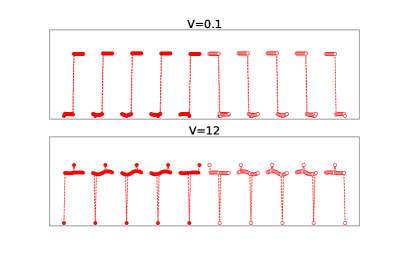
Figure 1: Schematic figure depicting the distribution functions, $m_{i}(j)$ $(i,j=1,...,L)$, defined at each point in the BZ for the two regimes of interaction, for 18 sites. The first five distributions depicted with filled circles represent distribution functions at alternate points for quasi-momenta modes inside the Fermi sea, $m_{k_{in}}$. While the remaining five depicted using unshaded circles represent distributions for quasi momenta modes outside it, $m_{k_{out}}$. In deep metallic regime, at $V=0.1$, the first five distributions are completely opposite of the next five. However, for deep insulating regime, at $V=12$, $m_{i}$ are almost identical for all $k_{i}\in k_{in},k_{out}$, differing only at points $i,i+\frac{L}{2}$.

Deep in the metallic regime, the above distributions $\{m_{i}(j)\}$ are completely opposite of each other for points inside Fermi sea and points outside it and exactly identical for all points inside (or outside) the Fermi sea. Whereas deep in insulating regime, the distribution for every point in the BZ are almost identical, differing only at the points $(i,i+\frac{L}{2})$ Hassan et al. (2018); Chakrabarti et al. (2019) ( Eq. 36). This is illustrated in the Fig. (1).

In the remaining part of this paper, we elaborate on how we analyse the geometry of the above distance distribution functions using the technique of optimal transport. In particular we study the construction of Wasserstein distances and investigate the underlying optimal transport theory in details in the context of quantum geometry of the correlated states. The geometrical observables thus obtained are found to sharply characterise the phases of the system.

III Theory of optimal transport and the Wasserstein distances

III.1 Review of the theory of optimal transport

In this section, we will review the theory of optimal transport, focussing on the context we will be applying it to, namely quantum geometry of the states of a 1-dimensional model of interacting fermions.

III.1.1 The Wasserstein distance

The theory of optimal transport defines distances between probability distribution functions Villani (2008, 2003) and thus allows us to compare a set of distance distribution functions quantitatively.

Optimal transport gives a definition of distance between two probability distribution functions (PDFs) $m_{i}$ and $m_{j}$, $W_{p}(m_{i},m_{j})$, as follows:

$$W_{p}^{(p)}(m_{i},m_{j})\equiv\inf_{\pi}\sum_{k,l}(\tilde{d}(k,l))^{p}\pi_{ij}(k,l),$$ (5)

where $k,l$ in the above sum runs over the domain of the PDFS, $p\in[1,\infty)$ and $\pi_{ij}(k,l)$ are joint probability distributions whose marginals are $m_{i}$ and $m_{j}$,

$$\sum_{l}\pi_{ij}(k,l)=m_{i}(k),~{}~{}\sum_{k}\pi_{ij}(k,l)=m_{j}(l).$$ (6)

The $p$th root of the above optimised function $W_{p}(m_{i},m_{j})$ satisfies all the axioms of a distance function only when $\tilde{d}(k,l)$ is a valid distance function and satisfies all the properties of a metric.

Physically, $\pi_{ij}(k,l)$ is usually interpreted as different ways to transport material such that the distribution function $m_{i}$ is transformed to the distribution function $m_{j}$. However, $(\tilde{d}(k,l))^{p}$ in a more general scenario, is called the cost function of the transport where it is not restricted to be positive powers of a valid distance and is interpreted as the cost paid for above transfer. Whereas the above optimised sum $W_{p}^{(p)}(m_{i},m_{j})$ is defined as the minimal cost of transforming $m_{i}$ to $m_{j}$. The central concept of above transport problem involves finding an optimal joint distribution function $\pi_{ij}^{*}(k,l)$ such that the sum defined on the RHS of Eq. 5 is minimum.

Choosing $p=2$ in Eq. 5, we define squared Wasserstein distances $W^{(2)}(m_{i},m_{j})$ between any two PDFs $m_{i}$ and $m_{j}$ as follows,

$$W^{(2)}(m_{i},m_{j})\equiv\inf_{\pi}\sum_{k,l}(\tilde{d}(k,l))^{2}\pi_{ij}(k,l).$$ (7)

Here $\pi_{ij}$ satisfies the constraints given by Eq. (6).

We consider the distributions, $m_{i}$ and $m_{j}$, to be the distance distributions defined in Section II.1 at any two points $k_{i}$ and $k_{j}$ on the BZ. While $\tilde{d}(k,l)$ can be any valid distance defined between the points in the BZ, we have studied the quantum distances and the Euclidean distances on the BZ (detailed later). The corresponding squared Wasserstein distance between the distance distributions, given by the above sum in Eq. (7) then gives the weighted average of all the squared distances between any two points in the BZ, with the corresponding weights given by the optimal joint probability distribution $\pi^{*}_{ij}$. The Wasserstein distance can be computed numerically using the standard techniques of linear programming Loisel and Romon (2014) by minimization of the linear function of $\pi_{ij}$, defined in Eq. (7), subject to linear constraints specified by Eq. (6).

III.2 The Wasserstien distance obtained from the quantum distance

In this section we study the geometry of the distance distributions (Sec. II.1) in terms of the Wasserstein distance obtained by choosing the square of the quantum distances (defined in Eq. (2)), as the cost function of the optimal transport problem. This is done by substituting these distances in Eq. (7). We first look at physical interpretation of above distances in terms of quantities in the Hilbert space, since our definition is derived completely from the quantum distances. Finally, we close this section by discussing the results obtained from analytical calculations at extreme limits of interaction and from the numerical linear programming solutions for intermediate interaction values, using the distance matrices given by exact diagonalization.

We define squared Wasserstein distances between two distance distributions $m_{i}$ and $m_{j}$ in terms of the matrix of quantum distances $D$ as follows,

$$W^{(2)}(m_{i},m_{j})\equiv\inf_{\pi}\sum_{k,l=1}^{L}(D(k,l))^{2}\pi_{ij}(k,l).$$ (8)

Where $\pi_{ij}$ satisfies the constraints given by Eq. 6. The above distance is closely related to the underlying geometry of the discrete metric space under investigation and is intricately related to the intrinsic curvature Ollivier (2009, 2010, 2013), as discussed in details in our previous work Chakrabarti et al. (2019).

III.2.1 Physical interpretation

In our context, namely the quantum geometry of many-fermion states, we have no concept of “transport”. We are studying the kinematics of many-fermion states and hence there is no time evolution. We are only analysing static correlation functions.

Thus, the physical interpretation of our application of the theory of optimal transport is quite different from the standard one discussed above. It is as detailed below.

The distance matrix defined in equation (2) can be written as,

$$(D(i,j))^{2} \equiv 1-{\rm Tr}\left(\hat{\rho}(i,j)\hat{\rho}_{0}\right)$$ (9)

$$\hat{\rho}_{0} \equiv |\psi\rangle\langle\psi|$$ (10)

$$\hat{\rho}(i,j) \equiv E(i,j)|\psi\rangle\langle\psi|E(i,j)$$ (11)

Thus, the distance matrix is defined in the subspace spanned by the states $E(i,j)|\psi\rangle\equiv|i,j\rangle$. We will call this subspace the quantum distance Hilbert space, $QDH$.

The minimisation of the sum defined on the RHS of
Eq. 8 gives us an optimal joint probability distribution function, $\pi_{ij}^{*}(k,l)$ for a set of distributions $m_{i}$ and $m_{j}$. We define mixed states, $\hat{\rho}^{\prime}(i,j)$ in $QDH$ by,

$$\hat{\rho}^{\prime}(i,j)\equiv\sum_{k,l}\pi_{ij}^{*}(k,l)|k,l\rangle\langle k,l|.$$ (12)

The squared Wasserstein distance $W^{(2)}(m_{i},m_{j})$ given by Eq. 8 can be rewritten as,

$$W^{(2)}(m_{i},m_{j})=1-Tr(\hat{\rho}_{0}\hat{\rho}^{\prime}).$$ (13)

III.2.2 Analytical and numerical results

In this section we present the results obtained from the analytical calculations with the known distances obtained from the ground state at the extreme limits of the interaction and the numerical results obtained for the distance matrices given by exact diagonalization, for interaction values $V=0-12$ and system sizes $L\leq 18$.

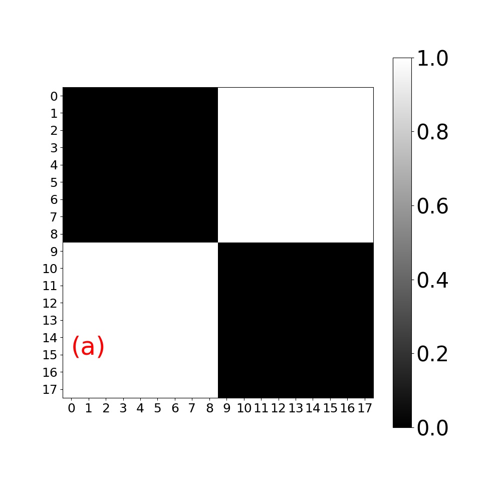
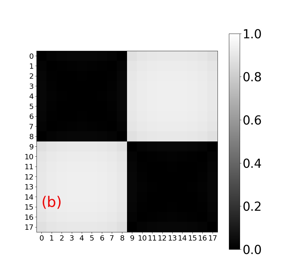
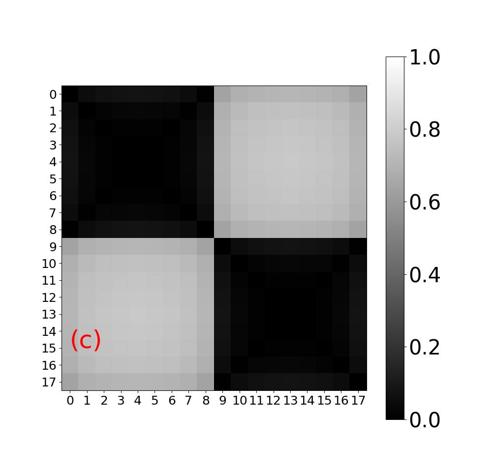
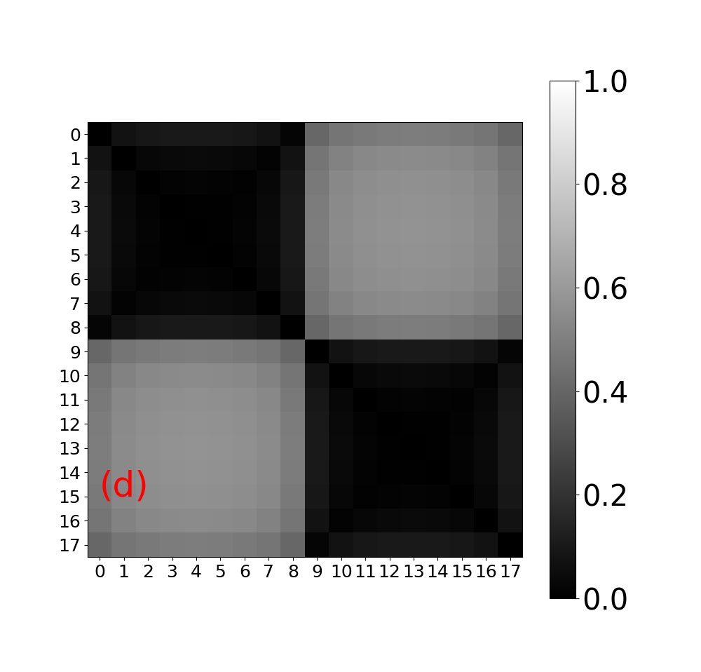
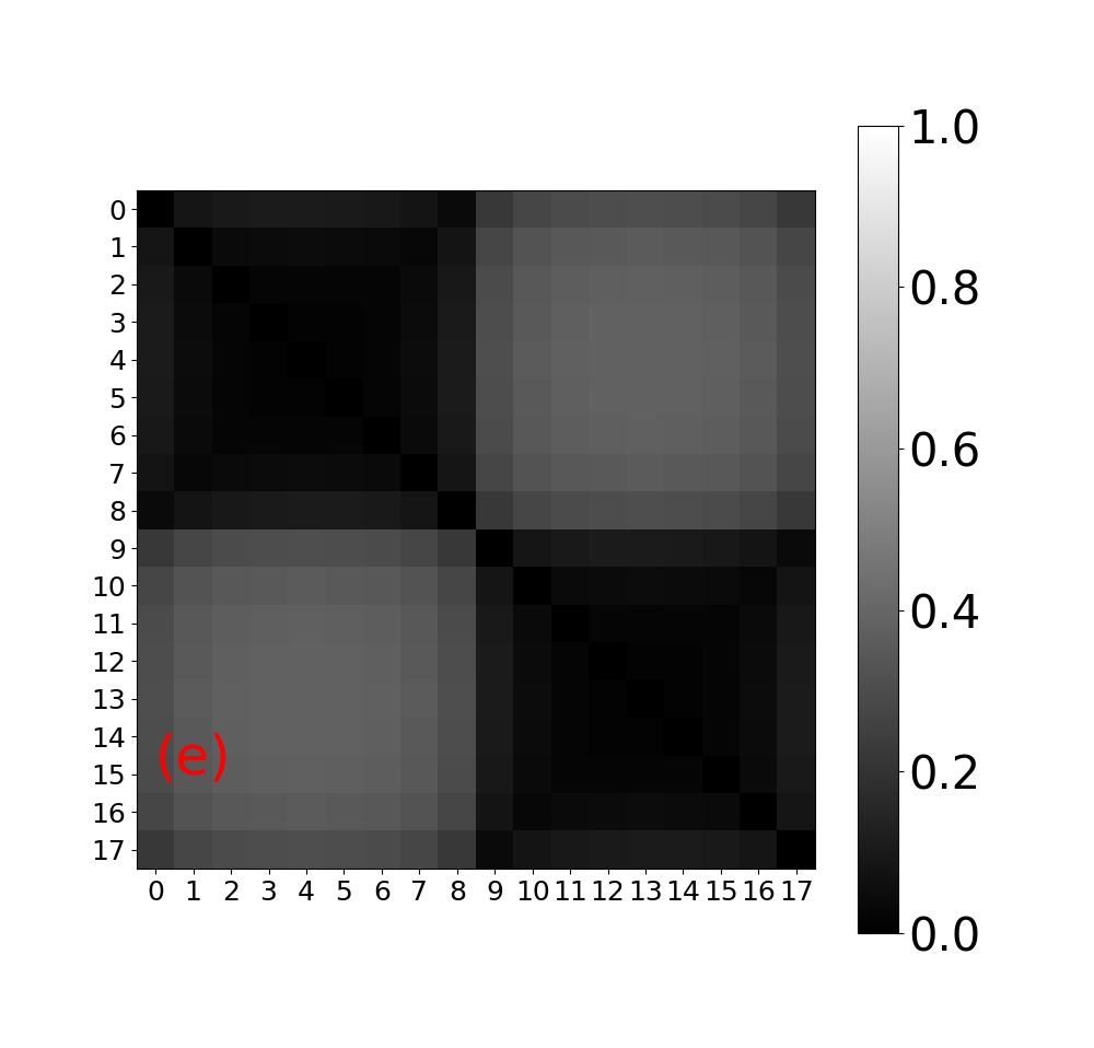
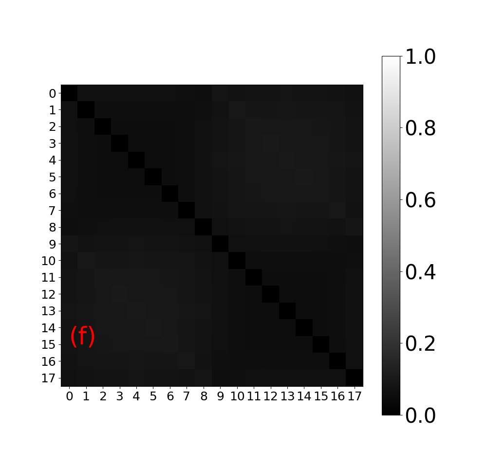
Figure 2: (a)-(f)Squared Wasserstein Distance matrices $W^{(2)}(m_{i},m_{j})$ for $L=18$, obtained from numerical computation for interaction strengths $V=0.1$ (a), $V=1$ (b), $V=2$ (c), $V=3$ (d), $V=4$ (e) and $V=12$ (f). For $i<9$, the quasi momenta modes lie inside the Fermi sea, $k_{i}\in k_{in}$ and for $i\geq 9$, the quasi-momenta modes lie outside it, $k_{i}\in k_{out}$. The deep metallic regime is characterised by $\sim 0,\sim 1$ distance values between $k_{in}-k_{in}$ ($k_{out}-k_{out}$) and $k_{in}-k_{out}$ blocks respectively. The deep insulating regime is characterised by uniform extremely small values very close to zero.

We denote the analytical quantum distances in the ground state at extreme values of coupling constant $V$ by $D_{V}(i,j)$ and the corresponding squared Wasserstein distances by $W^{(2)}_{V}(m_{i},m_{j})$. For the extreme limits of interaction we can then show that (calculations in VI)

$$W^{(2)}_{0}(m_{i},m_{j}) = (D_{0}(i,j))^{2}$$

$$W^{(2)}_{\infty}(m_{i},m_{j}) = \frac{1}{{\cal L}}(D_{\infty}(i,j))^{2}.$$ (14)

Starting from the $L$ distribution functions defined on the BZ, for a system with $L$ number of lattice sites, comparing every pair of distributions ($m_{i},~{}m_{j}$) we have a $L\times L$ matrix of squared Wasserstein distances $W^{(2)}(m_{i},m_{j})$. We look at the numerical $W^{(2)}$ matrices obtained for interaction values $0<V\leq 12$ in Fig. (2). We find a direct reflection of the features of the distribution functions observed in Sec. II.1. In deep metallic regime, the distance distributions for $k_{in}-k_{in}$ or $k_{out}-k_{out}$ being identical corresponding Wasserstein distances $W^{(2)}(m_{k_{in}},m_{k_{in}})$ (or $W^{(2)}(m_{k_{out}},m_{k_{out}})$) are very small ($\sim 0$). While, distributions for $k_{in}-k_{out}$ are completely opposite to each other and thus the Wasserstein distances $W^{(2)}(m_{k_{in}},m_{k_{out}})$ are very large ($\sim 1$). Whereas in deep insulating regime the distance distributions are homogenous and almost identical so the Wasserstein distances are uniform and almost zero.

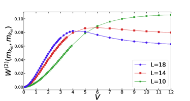
Figure 3: Squared Wasserstein distances between quasi-momenta modes inside the Fermi sea, $W^{(2)}(m_{k_{in}},m_{k_{in}})$, as a function of the interaction strength $V$ for system sizes $L=10,14,18$.

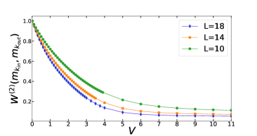
Figure 4: Squared Wasserstein distances between quasi-momenta modes inside the Fermi sea and those outside it, $W^{(2)}(m_{k_{in}},m_{k_{out}})$, as a function of the interaction strength $V$ for system sizes $L=10,14,18$.

We look at the behaviour of the distances $W^{(2)}(m_{k_{in}},m_{k_{in}})$ and $W^{(2)}(m_{k_{in}},m_{k_{out}})$, as a function of the interaction strength $V$ for different system sizes in Fig. (3) and Fig. (4) respectively. From Fig. (3) we can expect $W^{(2)}(m_{k_{in}},m_{k_{out}})$ to indicate the critical interaction strength for the Luttinger liquid to CDW transition Shankar (1990), by the occurence of a peak in the thermodynamic limit.

We numerically compute the Wasserstein distances in an ideal CDW phase starting from the distance distributions as given by the analytical distance matrices at $V=\infty$ (Eq. 36) for system sizes $L=10-28$. We denote the above uniform squared distances by $W_{\infty}^{(2)}$ and study its behaviour as a function of the inverse of system size in Fig. 5. It is found to be linear in $L^{-1}$ and thus vanishes in the thermodynamic limit, as also predicted by Eq. 14. The same result is indicated by Fig. (3) and Fig. (4) for $V\succsim 4$, in the insulating phase. While Eq. (14) and Fig. (4) suggest that the Wasserstein distances are non-zero for the metallic phase, in the thermodynamic limit.

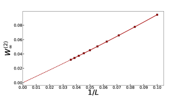
Figure 5: $W_{\infty}^{(2)}$ as a function of the inverse system size $L^{-1}$ for system sizes $L=10-28$. It is found to be linear in $L^{-1}$ and thus vanishes in the thermodynamic limit.

From the above results we conclude, the Wasserstein distance gives a vivid geometric description of the ground state in both the phases. It characterises the geometry of the distance distributions extremely well. It characterises the metallic phase by classifying the points inside the Fermi sea and those outside it in two different groups, while it characterises the insulating phase by homogenous values. The most striking finding is that in the thermodynamic limit, the Wasserstein distance becomes zero in the insulating phase while it is non-zero in the metallic phase. Thus it provides a sharp characterisation of the phases of the system.

III.3 The Wasserstien distance obtained from the Euclidean distance

In this section we propose a definition for Wasserstein distances in terms of the Euclidean distances between the quasi-momenta in the BZ, by choosing the square of the Euclidean distances as the cost function of the optimal transport problem and substituting these distances in Eq. (7). We then look at the numerical results and observations.

We define the squared Wasserstein distance between two distance distributions $m_{i}$ and $m_{j}$, $W_{E}^{(2)}(m_{i},m_{j})$, as follows:

$$W_{E}^{(2)}(m_{i},m_{j})\equiv\inf_{\pi}\sum_{k,l=1}^{L}(k-l)^{2}\pi_{ij}(k,l),$$ (15)

where $\pi_{ij}$ satisfies the constraints given by Eq. 6.

The above distance compares the distance distributions and equips us with means to study the geometry of the distance distributions and thus the rich physical transformation emerging as a function of the interaction (Sec. II.1). However, we cannot connect it to quantities in the Hilbert space immediately as the distance function is no longer derived from states in the Hilbert space. It can neither be connected to the intrinsic curvature as before. But it is still interesting physically, because it probes the geometry of the distance distribution functions derived from the quantum distances.

III.3.1 Numerical results

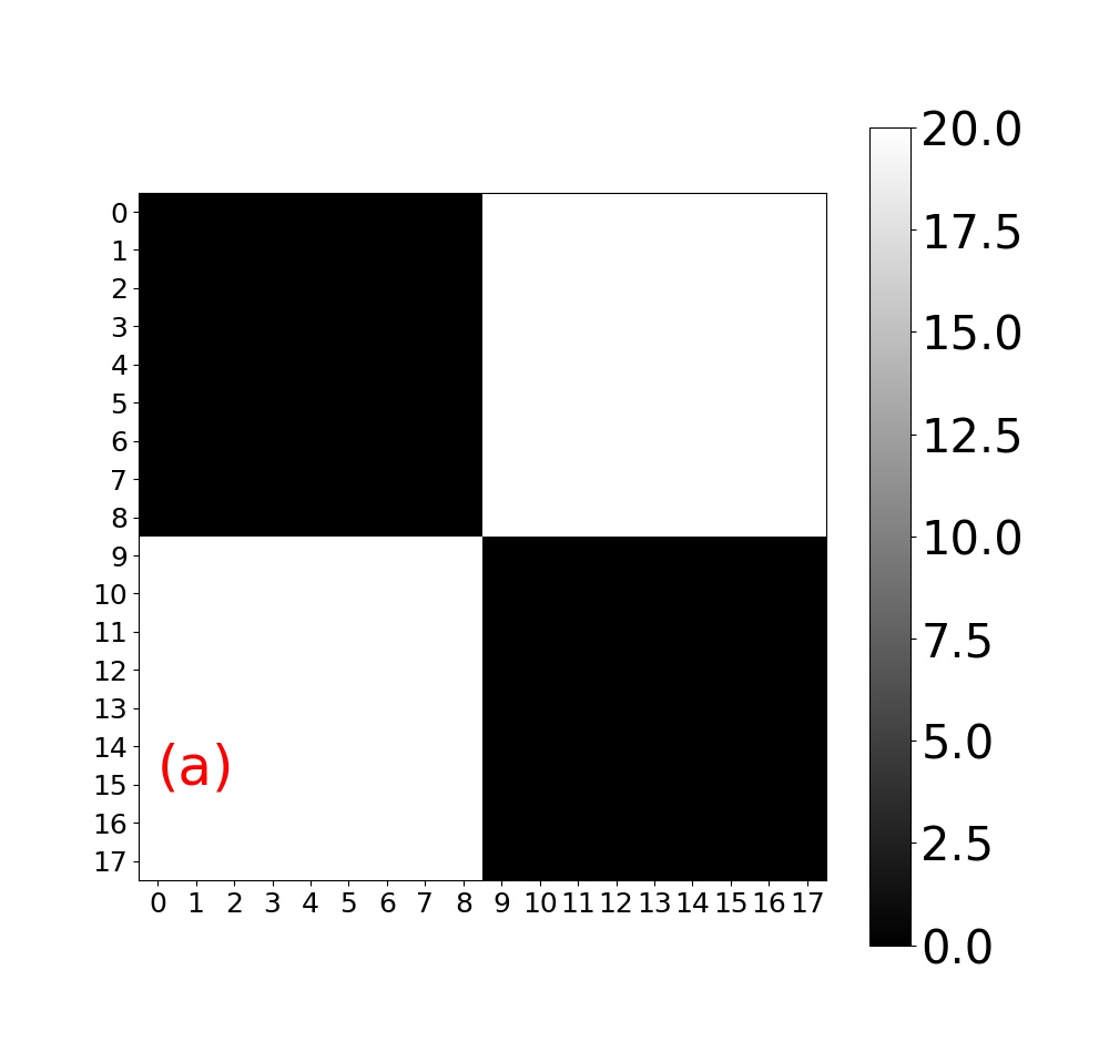
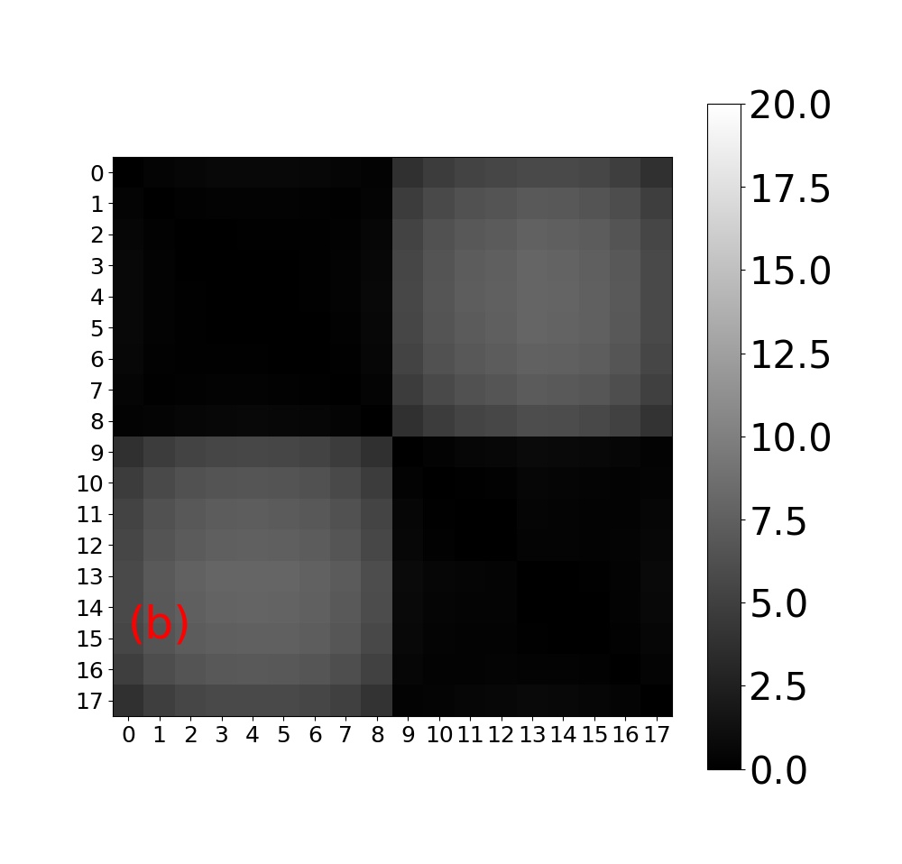
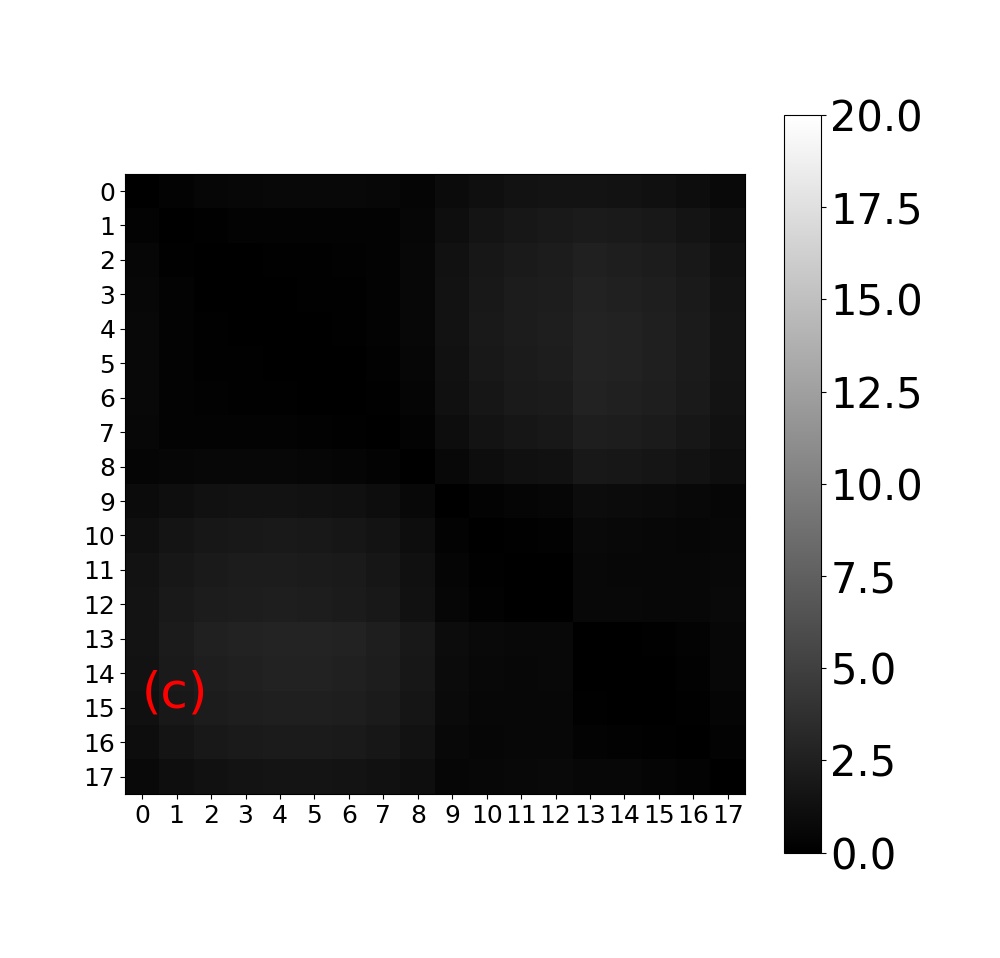
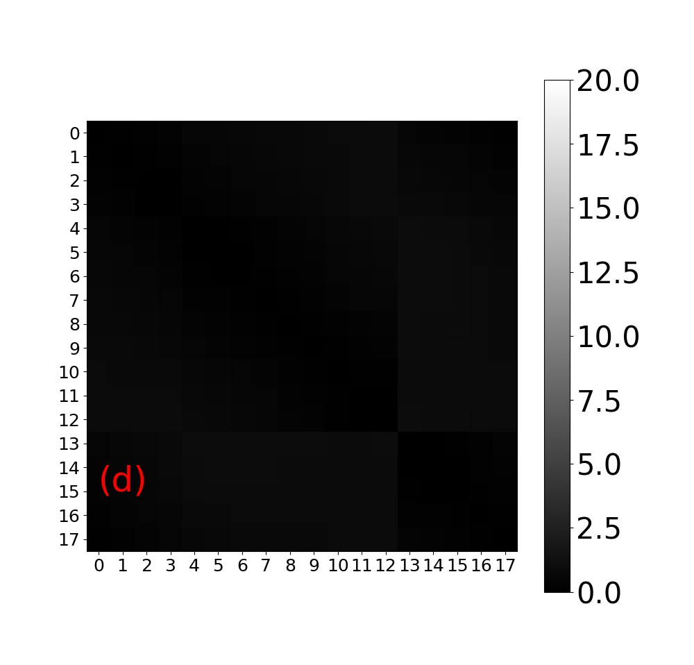
Figure 6: (a)-(d)Squared Wasserstein Distance matrices $W_{E}^{(2)}(m_{i},m_{j})$ for $L=18$, obtained from numerical computation for interaction strengths $V=0.1$ (a), $V=2$ (b), $V=4$ (c), and $V=12$ (d). For $i<9$, the quasi momenta modes lie inside the Fermi sea, $k_{i}\in k_{in}$ and for $i\geq 9$, the quasi-momenta modes lie outside it, $k_{i}\in k_{out}$. The deep metallic regime is characterised by $\sim 0,\sim 20$ distance values between $k_{in}-k_{in}$ ($k_{out}-k_{out}$) and $k_{in}-k_{out}$ blocks respectively. The deep insulating regime is characterised by uniform and extremely small values.

In this section we discuss the results obtained numerically from the linear programming solutions of the optimal transport problem, choosing the marginals to be the distribution functions constructed from the distance matrices obtained by performing exact diagonalization.

We look at the numerical $W_{E}^{(2)}$ matrices obtained for interaction values $0<V\leq 12$ in Fig. (6). We find the overall behaviour is quite similar to the observations found for the Wasserstein distances obtained from the quantum distances in Sec. III.2. Like before, in deep metallic regime the Wasserstein distances classify the points inside and outside the Fermi sea into two different categories, reflecting the geometry of the distance distributions (Secs. II.1 and III.2). The Wasserstein distances $W_{E}^{(2)}(m_{k_{in}},m_{k_{in}})$ (or $W_{E}^{(2)}(m_{k_{out}},m_{k_{out}})$) are very small ($\sim 0$), while $W^{(2)}_{E}(m_{k_{in}},m_{k_{out}})$ are very large ($\sim 20$). Whereas, in deep insulating regime the Wasserstein distances are uniform and very small.

We look at the behaviour of the distances $W_{E}^{(2)}(m_{k_{in}},m_{k_{in}})$ and $W_{E}^{(2)}(m_{k_{in}},m_{k_{out}})$, as a function of the interaction strength $V$ for different system sizes in Fig. (7) and Fig. (8) respectively. The above distances sense the metal-insulator transition very distinctively and indicate a critical interaction strength $V_{c}=2.4$, which is very close to the theoretical value Shankar (1990). $W_{E}^{(2)}(m_{k_{in}},m_{k_{in}})$ indicates the transition by a peak, which we expect to be more sharpened in the thermodynamic limit. In the regime $V\precsim 2.4$, $W_{E}^{(2)}(m_{k_{in}},m_{k_{out}})$ rapidly reduces with the increase of interaction, moreover it scales proportionately with the system size, post which it is insensitive to the system size and constant as a function of the interaction. Thus $W_{E}^{(2)}(m_{k_{in}},m_{k_{out}})$ is expected to diverge in the metallic phase and remain finite in the insulating phase.

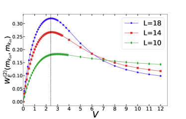
Figure 7: Squared Wasserstein distances between quasi-momenta modes inside the Fermi sea, $W_{E}^{(2)}(m_{k_{in}},m_{k_{in}})$, as a function of the interaction strength $V$ for system sizes $L=10,14,18$. The above distances show a prominent peak at $V=2.4$, for $L>10$.

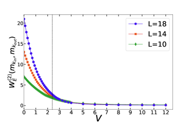
Figure 8: Squared Wasserstein distance between quasi-momenta modes inside the Fermi sea and those outside it, $W_{E}^{(2)}(m_{k_{in}},m_{k_{out}})$, as a function of the interaction strength $V$ for system sizes $L=10,14,18$. For $V\precsim 2.4$, above distance scales proportionately with the system size, post which it is insensitive to the system size.

Summarising the results we can say that the Wasserstein distance obtained from the Euclidean distances in the BZ is able to characterise the geometry of the distance distributions extremely well and thus provides a detailed geometric characterisation of the geometry of the ground state in both the phases. It is able to indicate a critical value of interaction $V_{c}=2.4$ for the metal-insulator transition, which is very close to the theoretical value Shankar (1990), $V=2$. Moreover it is able to differentiate the metallic and insulating phases because the distances between the quasi-momenta modes inside the Fermi sea and those outside it are divergent in the metallic phase and finite in the insulating phase.

IV The Wasserstein barycenter

In the previous sections starting from $L$ distance distributions $\{m_{i}(k)\}$ at each point $k_{i}~{}(i=1,...L)$ on the BZ we studied the Wasserstein distances defined between every pair of distibutions and found it very efficiently captures the physics of the system. However, the $L\times L$ matrix of Wasserstein distances have $L_{C_{2}}$ independent elements. Thus we further face the question, how to identify a single order parameter which can identify the metallic and insulating phases well. We address this question in this section by applying the concept of Wasserstein barycenter Agueh and Carlier (2011); Cuturi and Doucet (2014).

In geometry, for a configuration of points the barycenter usually implies the arithmetic mean of the coordinates. We begin with the question that analogously for above configuration of $L$ distance distributions whether there is some way of obtaining a single average distribution on the BZ which can efficiently characterise the configuration. In Euclidean case Sturm (2002), for a collection of points $(x_{1},...,x_{p})$, the barycenter $x^{*}$, is obtained by minimising the function $\sum_{i=1}^{p}\lambda_{i}\mid x-x_{i}\mid^{2}$, where $\lambda_{i}\in[0,1]$ and $\sum_{i=1}^{p}\lambda_{i}=1$ .

Optimal transport generalizes the same concept to a collection of probability distributions by considering the weighted sum of squared Wasserstein distances instead of the above weighted sum of the squared Euclidean distances and introducing a single distribution function which minimizes the above sum Agueh and Carlier (2011). The barycenter $m^{*}(k)$ is defined as a single function on the BZ such that the average sum of the squared Wasserstein distances between the function and each of the distributions (sum defined on the RHS of Eq. 16), is minimised. We define a single geometric parameter, the average squared Wasserstein distance between the barycenter and the distance distributions, as the follows,

$$J(m^{*})\equiv\inf_{m}\frac{1}{L}\sum_{i=1}^{L}W^{(2)}(m_{i},m),$$ (16)

where we take all the weights to be uniform for simplicity. For computation of the Wasserstein barycenter we use the entropic regularisation of the optimal transport problem Cuturi (2013). In above method, the solution for the barycenter is obtained by minimising the average sum of squared regularised Wasserstein distances $W^{(2)}_{\gamma}(m_{i},m)$, defined by the following equation,

$$W^{(2)}_{\gamma}(m_{i},m) \equiv \inf_{\pi}(\sum_{ij}(D(i,j))^{2}\pi^{i}_{\gamma}(i,j)+\gamma S(\pi^{i}_{\gamma}))$$ (17)

$$S(\pi^{i}_{\gamma}) \equiv \sum_{kl}\pi^{i}_{\gamma}(k,l)log(\pi^{i}_{\gamma}(k,l)).$$ (18)

Where $\pi^{i}_{\gamma}(i,j)$ are the joint probability distributions with marginals $m_{i}$ and $m$, $\gamma$ is a positive regularisation parameter which is also a measure of the error introduced in the Wasserstein distance and $D(i,j)$ is the matrix of the quantum distances.The second term on the RHS corresponds to the entropy of above $\pi^{i}_{\gamma}(i,j)$ matrix. The regularised Wasserstein distances, can be computed by applying Sinkhorn-Knopp’s fixed point iteration algorithm Sinkhorn and Knopp (1967); Knight (2008).

IV.1 Numerical Results

In this section we look at the numerical results obtained by taking the $18$ distance distribution functions constructed from the quantum distances and computing the corresponding barycenter, defined in terms of the squared regularised Wasserstein distances $W^{(2)}_{\gamma}(m_{i},m)$ given by Eq. (17), for a choice of the regularising parameter $\gamma=0.006$.

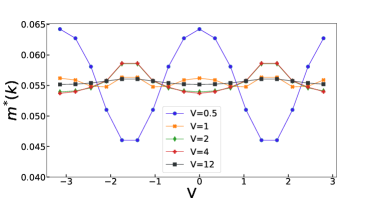
Figure 9: The barycenter $m^{*}(k)$ defined over the BZ, $k\in[-\pi,\pi)$, for different interaction values. The Fermi points are $k_{f}=\pm\frac{\pi}{2}$. We find that in deep metallic phase $m^{*}(k)$ is highly inhomogenous over the BZ and $m^{*}(k_{f})$ is minimum. While in the deep insulating phase the distribution is flat and homogenous.

We plot the barycenter over the BZ, for different interaction values in Fig.(9). The distribution is highly inhomogeneous over the quasi-momenta modes in the metallic phase. For large $V$, in deep insulating phase we observe a contrasting homogenous behaviour.

In the entropic regularisation method of the optimal transport, as discussed earlier, minimisation of the RHS of Eq. (17), gives us an optimal but approximate joint distribution $\pi^{i*}_{\gamma}(k,l)$ which however is very close to the actual $\pi^{i*}(k,l)$ for the extremely small value of regularisation parameter we choose, $\gamma=0.006$. Thus average of the squared quantam distances over the BZ given by above joint probability distribution $\pi^{*i}_{\gamma}(k,l)$, will be very close to the squared Wasserstein distances $W^{(2)}(m_{i},m)$ given by Eq. 8. So after obtaining the optimal joint distribution $\pi^{i*}_{\gamma}(k,l)$ by applying Sinkhorn-Knopp’s fixed point iteration algorithm Sinkhorn and Knopp (1967); Knight (2008), we redefine the corresponding squared regularised Wasserstein distances $\tilde{W}^{(2)}_{\gamma}(m_{i},m^{*})$, as follows:

$$\tilde{W}^{(2)}_{\gamma}(m_{i},m^{*})\equiv\sum_{kl}(D(k,l))^{2}\pi^{i*}_{\gamma}(k,l).$$ (19)

The corresponding average squared Wasserstein distance between the barycenter and the configuration of $18$ distributions, $\tilde{J}(m^{*})$ can then be defined as,

$$\tilde{J}(m^{*})\equiv\frac{1}{L}\sum_{i}(\sum_{kl}(D(k,l))^{2}\pi^{i*}_{\gamma}(k,l)).$$ (20)

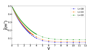
Figure 10: Average squared Wasserstein distance between the distribution functions and the barycenter as a function of the interaction strength, for different system sizes.

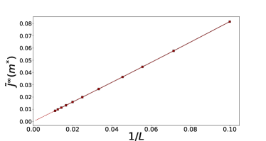
Figure 11: Average squared Wasserstein distance between the distribution functions and the barycenter at the extreme interaction limit, $V=\infty$ for system sizes $L=10-100$, as a function of the inverse of system size.

We have looked at the behaviour of $\tilde{J}(m^{*})$ as a function of the interaction strength and compared system sizes $L=10,14,18$, like before, in Fig. (10). We find it abruptly reduces with increase of interaction strength in the metallic phase and becomes very small and rather insensitive to the interacion in the deep insulating phase. Moreover it is insensitive to the system size in deep metallic phase and reduces with increase of system size in deep insulating phase. We compute $\tilde{J}(m^{*})$ for the CDW interacion limit, $V=\infty$, by constructing the distributions from the analytical distance matrix (36), for system sizes $L=10-100$ and label it as $\tilde{J}^{\infty}(m^{*})$. It is found to be linear in $L^{-1}$ as demonstrated in Fig. 11, similar to the Wasserstein distances defined in terms of the quantum distances in Sec. III.2.

In early metallic phase, with the distributions being drastically different for points inside and outside the Fermi sea, we would expect the barycenter to be very different from the starting parent distributions and corresponding average squared Wasserstein distance between the barycenter and the distance distributions would be appreciable. However the insulating phase being characterised by more or less identical distributions, the barycenter should also be an uniform distribution on the BZ and the average Wasserstein distance from the parent distributions should be negligible in the thermodynamic limit. The above results provide strong evidences of the same. The average Wasserstein distance between the barycenter and the distance distributions becomes zero in the insulating phase and is non-zero in the metallic phase. It can be considered as a single geometrical observable which is able to characterise the phases.

V Discussion and conclusions

As stated in the introduction (I), this paper along with two previous ones Hassan et al. (2018); Chakrabarti et al. (2019) constitutes our attempt, following previous work Kohn (1964); Resta and Sorella (1999); Sgiarovello et al. (2001); Marrazzo and Resta (2017); Resta (2011) to formulate a new approach to the geometric characterization of insulating and metallic states. We first summarize our results.

In our first work Hassan et al. (2018), we had given a mathematically consistent definition of the quantum distances between two points in the spectral parameter space for a general many-fermion state. The quantum distances can be obtained by computation of the static correlation functions applying any exact or approximate technique like quantum Monte Carlo methods, DMRG and bosonisation in one dimension, exact diagonalisation for finite systems, perturbation theory etc.. We were motivated by previous work Resta and Sorella (1999); Sgiarovello et al. (2001); Marrazzo and Resta (2017); Resta (2011) which had related the concept of quantum distances to Kohn’s seminal work Kohn (1964) of understanding the structure of insulating states in terms of quantum geometry. Thus, we chose to implement and study our formalism in the 1-dimensional $t-V$ model, for reasons detailed in the introduction (I). We found Hassan et al. (2018) that the distance matrix is qualitatively different in the metallic and insulating regimes.

In the following paper Chakrabarti et al. (2019), in an attempt to sharpen the difference, we investigated the extrinsic and instinric geometry implied by the distance matrix. We found that the intrinsic curvature, defined using the theory of optimal transport Ollivier (2009, 2010, 2013) and approximate Euclidean embedding of the Wasserstein distances seem to be the better discriminants .

Hence, in this paper we have focussed on applying the theory of optimal transport Villani (2008, 2003) to analyse the quantum distance matrix of the 1 dimensional $t-V$ model. We have obtained the following results.

We construct a geometric quantity, the matrix of Wasserstein distances that distinguishes sharply between the metallic and insulating states, in the thermodynamic limit. The Wasserstein distances defined in terms of the quantum distances are zero in the insulating phase and non-zero in the metallic phase, while the Wasserstein distances defined in terms of the Euclidean distances on the BZ, between the quasi-momenta modes inside the Fermi sea and those outside it are divergent in the metallic phase and finite in the insulating phase.

The matrices of quantum distances and Wassertein distances are functions of a pair of points in the spectral parameter space. It is clearly useful to identify a single parameter to discriminate between the metallic and insulating states. We have shown that the concept of the Wasserstein barycenter Agueh and Carlier (2011), occuring in the theory of optimal transport, precisely does this.

Thus, in the context of the one dimensional $t-V$ model, we have shown that the geometric entities constructed using the theory of optimal transport give a sharp distinction between the metallic and the insulating state.

It is therefore reasonable to infer that the theory of optimal transport, in general is a good way to extract the physically relevant geometric quantities of any correlated state. We would like to stress that it is not our claim that by the procedure we adopted in these papers to analyse the metalllic and insulating states we could observe a general characterisation for all physical situations. Each problem will have to be analysed individually. However, the general feature of this technique, that it enables the extraction of geometric quantities averaged over the BZ, lead us to propose that it will be useful in other physical contexts as well.

Our new approach to study the structure of a many-body state is closely related with the machine learning approach towards data analysis. We generate probability distribution functions from the many body state and by comparing these distributions ( in terms of Wasserstein distance) we infer geometric properties of ground state. Similarly, in machine learning one often has to deal with collections of samples that can be interpreted as probability distributions. Comparing, summarising, and reducing the dimensionality of the probability distributions on a given metric space are fundamental tasks in statistics and machine learning. The Wasserstein distance is increasingly being used in machine learning and statistics Cuturi (2013); Kolouri et al. (2017); Arjovsky et al. (2017); Courty et al. (2015); Kusner et al. (2015), especially for its way of comparing distributions based on basic principles.

In conclusion, we propose that, in general, physically relevant geometric information about correlated states can be extracted from the matrix of quantum distances using the techniques from the theory of optimal transport.

VI Acknowledgements

We are grateful to R. Simon, S. Ghosh, R. Anishetty, A. Samal and Emil Saucan for useful discussions.

Appendix A The extreme limits

In this section, we present analytic proofs for the results stated in the text (Eq. s III.2.2) for $W(m_{i},m_{j})$ in the extreme limits of the coupling. Namely, $V=0$ and $V=\infty$.

A.1 $V=0$

The distance matrix at $V=0$ is easily computed Hassan et al. (2018). It can be written as

$$D=\left(\begin{array}[]{cc}0&{\cal I}\\ {\cal I}&0\end{array}\right)$$ (21)

where ${\cal I}$ is the $L/2\times L/2$ matrix with all entries equal to 1. We denote the $L/2$ component column vector with all entries equal to 1 by $e$. We represent the distance distributions defined in Equation 4 by column vectors $m_{i},m_{L/2+i},i=1,\dots,L/2$,

$$m_{i}=\frac{2}{L}\left(\begin{array}[]{c}0\\ e\end{array}\right)~{}~{}~{}~{}~{}m_{L/2+i}=\frac{2}{L}\left(\begin{array}[]{c}e\\ 0\end{array}\right).$$ (22)

The constraints defining the joint probability distributions, $\pi_{ij}$ can be writen in a matrix form,

$$\pi_{ij}\left(\begin{array}[]{c}e\\ e\end{array}\right)=m_{i}~{}~{}~{}~{}\left(\begin{array}[]{cc}e^{T}&e^{T}\end{array}\right)\pi_{ij}=m^{T}_{j}.$$ (23)

The general solution to the above equations(23) is

$$\pi_{ij}=\frac{2}{L}\left(\begin{array}[]{cc}0&0\\ 0&P\end{array}\right)~{}~{}~{}~{}\pi_{iL/2+j}=\frac{2}{L}\left(\begin{array}[]{cc}0&0\\ P&0\end{array}\right)$$ (28)

$$\pi_{L/2+ij}=\frac{2}{L}\left(\begin{array}[]{cc}0&P\\ 0&0\end{array}\right)~{}~{}~{}~{}\pi_{L/2+iL/2+j}=\frac{2}{L}\left(\begin{array}[]{cc}P&0\\ 0&0\end{array}\right),$$ (33)

where $i,j=1,\dots,L/2$. $P$ is any $L/2\times L/2$ component positive semi-definite matrix whose rows and columns sum up to 1. $P(i,j)\geq 0,~{}\sum_{k=1}^{L/2}P(k,l)=1=\sum_{l=1}^{L/2}P(k,l)$.

The Wasserstein distances can be written in this matrix form as,

$$W(m_{i},m_{j})=\inf_{\pi}{\rm Tr}\left(D^{(2)}\pi_{ij}\right),$$ (34)

where $D^{(2)}(k,l)=(D(k,l))^{2}$. Using the fact that $P{\cal I}={\cal I}={\cal I}P$, it is easy to see that the RHS of the above equation is independent of P and we obtain the result stated in equation(III.2.2), that at $V=0$,

$$W(m_{i},m_{j})=(D(i,j))^{2}.$$ (35)

A.2 $V=\infty$

The distance matrix in the limit $V=\infty$ is Hassan et al. (2018),

$$D=c\left(\begin{array}[]{cc}{\cal I}-I&{\cal I}\\ {\cal I}&{\cal I}-I\end{array}\right)+(1-c)\left(\begin{array}[]{cc}0&I\\ I&0\end{array}\right),$$ (36)

where $c=\sqrt{3}/2$. To represent the distance distributions as column vectors, we define a set of $L/2$ component column vectors, $\chi_{i},i=1,\dots,L/2$ whose entries are all zero except for the $i^{\rm th}$ one, which is equal to 1. Namely, $\chi_{i}(j)=\delta_{ij}$. We then have,

$$m_{i}=\frac{1}{\cal L}\left(\begin{array}[]{c}ce-c\chi_{i}\\ ce+(1-c)\chi_{i}\end{array}\right),~{}~{}~{}~{}m_{L/2+i}=\frac{1}{\cal L}\left(\begin{array}[]{c}ce+(1-c)\chi_{i}\\ ce-c\chi_{i}\end{array}\right)$$ (37)

where ${\cal L}=c(L-2)+1$. We present a set of solutions to equations. We have no proof that these are the most general solutions. However, the definition of the Wasserstein distance in equation(34) implies that the infimum in this set provides an upper bound for $W(m_{i},m_{j})$. The solutions are of the form,

$$\pi_{ij}=\frac{1}{\cal L}\left(cP_{ij}+\pi^{\prime}_{ij}\right)$$ (38)

where $P_{ij}$ are $L\times L$, positive semi-definite matrices whose columns and rows sum up to 1.

$$P_{ij}\geq 0,~{}\sum_{k=1}^{L}P_{ij}(k,l)=1=\sum_{l=1}^{L}P_{ij}(k,l)$$ (39)

$\pi^{\prime}_{ij}$ are,

$$\pi^{\prime}_{ij} = \left(\begin{array}[]{cc}-c\chi_{i}\chi^{T}_{j}&0\\ 0&(1-c)\chi_{i}\chi^{T}_{j}\end{array}\right)$$ (42)

$$\pi^{\prime}_{iL/2+j} = \left(\begin{array}[]{cc}0&-c\chi_{i}\chi^{T}_{j}\\ (1-c)\chi_{i}\chi^{T}_{j}&0\end{array}\right)$$ (45)

$$\pi^{\prime}_{L/2+ij} = \left(\begin{array}[]{cc}0&(1-c)\chi_{i}\chi^{T}_{j}\\ -c\chi_{i}\chi^{T}_{j}&0\end{array}\right)$$ (48)

$$\pi^{\prime}_{L/2+iL/2+j} = \left(\begin{array}[]{cc}(1-c)\chi_{i}\chi^{T}_{j}&0\\ 0&-c\chi_{i}\chi^{T}_{j}\end{array}\right)$$ (51)

Equations (38), (LABEL:piinfans2) and the constraint $\pi_{ij}(k,l)\geq 0,k,l=1,\dots,L$, implies that $P_{ij}(i,j)-1\geq 0$. Since the maximum value of the matrix elements of $P_{ij}$ is 1, we have,

$$P_{ij}(i,j)=1,~{}~{}~{}~{}P_{ij}(i,k)=0~{}\forall k\neq j,~{}~{}~{}~{}P_{ij}(k,j)=0~{}\forall k\neq i.$$ (53)

Consider the set of matrices, $P^{*}_{ij}$ defined as,

$$P^{*}_{ij}(k,l)\equiv\delta_{kl}\left(1-\delta_{ik}-\delta_{jl}\right)+\delta_{ik}\delta_{jl}+\delta_{il}\delta_{jk},$$ (54)

it is straightforward to verify that $P^{*}_{ij}$ satisfy all the constraints in equations (39) and (53).

Thus, equations (34) and (38) imply,

$$W(m_{i},m_{j})\leq\frac{1}{\cal L}{\rm Tr}\left(D^{(2)}\left(cP^{*}_{ij}+\pi^{\prime}_{ij}\right)\right).$$ (55)

The RHS of the above inequality can be computed using equations (36), (LABEL:piinfans2) and (54). The result is,

$${\rm Tr}\left(D^{(2)}\left(cP^{*}_{ij}+\pi^{\prime}_{ij}\right)\right)=(D(i,j))^{2}.$$ (56)

Thus, we have proved the result stated in equation III.2.2, that at $V=\infty$,

$$W(m_{i},m_{j})\leq\frac{1}{\cal L}(D(i,j))^{2}.$$ (57)

References

- Hassan et al. (2018) S. R. Hassan, R. Shankar, and A. Chakrabarti, Phys. Rev. B 98, 235134 (2018).
- Chakrabarti et al. (2019) A. Chakrabarti, S. R. Hassan, and R. Shankar, Phys. Rev. B 99, 085138 (2019).
- Kohn (1964) W. Kohn, Phys. Rev. 133, A171 (1964).
- Resta and Sorella (1999) R. Resta and S. Sorella, Phys. Rev. Lett. 82, 370 (1999).
- Sgiarovello et al. (2001) C. Sgiarovello, M. Peressi, and R. Resta, Phys. Rev. B 64, 115202 (2001).
- Souza et al. (2000) I. Souza, T. Wilkens, and R. M. Martin, Phys. Rev. B 62, 1666 (2000).
- Marrazzo and Resta (2017) A. Marrazzo and R. Resta, Phys. Rev. B 95, 121114 (2017).
- Resta (2011) R. Resta, The European Physical Journal B 79, 121 (2011).
- Bures (1969) D. Bures, Trans. Amer. Math. Soc. 135, 199 (1969).
- Villani (2008) C. Villani, Optimal Transport: Old and New, 2009th ed., Grundlehren der mathematischen Wissenschaften (Springer, 2008).
- Villani (2003) C. Villani, Topics in Optimal Transportation, Graduate studies in mathematics (American Mathematical Society, 2003).
- Kolouri et al. (2017) S. Kolouri, S. R. Park, M. Thorpe, D. Slepcev, and G. K. Rohde, IEEE Signal Processing Magazine 34, 43 (2017).
- Agueh and Carlier (2011) M. Agueh and G. Carlier, SIAM Journal on Mathematical Analysis 43, 904 (2011), https://doi.org/10.1137/100805741 .
- Cuturi (2013) M. Cuturi, in Proceedings of the 26th International Conference on Neural Information Processing Systems - Volume 2, NIPS’13 (Curran Associates Inc., USA, 2013) pp. 2292–2300.
- Arjovsky et al. (2017) M. Arjovsky, S. Chintala, and L. Bottou, in Proceedings of the 34th International Conference on Machine Learning, Proceedings of Machine Learning Research, Vol. 70, edited by D. Precup and Y. W. Teh (PMLR, International Convention Centre, Sydney, Australia, 2017) pp. 214–223.
- Courty et al. (2015) N. Courty, R. Flamary, D. Tuia, and A. Rakotomamonjy, CoRR abs/1507.00504 (2015), arXiv:1507.00504 .
- Buttazzo et al. (2012) G. Buttazzo, L. De Pascale, and P. Gori-Giorgi, Phys. Rev. A 85, 062502 (2012).
- Cotar et al. (2013) C. Cotar, G. Friesecke, and C. Klüppelberg, Communications on Pure and Applied Mathematics 66, 548 (2013), https://onlinelibrary.wiley.com/doi/pdf/10.1002/cpa.21437 .
- Yang and Yang (1966) C. N. Yang and C. P. Yang, Phys. Rev. 150, 321 (1966).
- Baxter (1982) R. J. Baxter, Exactly Solved Models in Statistical Mechanics (Academic Press, 1982).
- Cazalilla et al. (2011) M. A. Cazalilla, R. Citro, T. Giamarchi, E. Orignac, and M. Rigol, Rev. Mod. Phys. 83, 1405 (2011).
- Loisel and Romon (2014) B. Loisel and P. Romon, Axioms 3, 119 (2014).
- Ollivier (2009) Y. Ollivier, Journal of Functional Analysis 256, 810 (2009).
- Ollivier (2010) Y. Ollivier, Probabilistic Approach to Geometry 57 (2010).
- Ollivier (2013) Y. Ollivier, Analysis and Geometry of Metric Measure Spaces: Lecture Notes of the 50th Séminaire de Mathématiques Supérieures (SMS), Montréal, 2011, edited by A. S. Galia Dafni, Robert McCann (AMS, 2013) pp. 197–219.
- Shankar (1990) R. Shankar, International Journal of Modern Physics B 04, 2371 (1990).
- Cuturi and Doucet (2014) M. Cuturi and A. Doucet, in Proceedings of the 31st International Conference on Machine Learning, Proceedings of Machine Learning Research, Vol. 32, edited by E. P. Xing and T. Jebara (PMLR, Bejing, China, 2014) pp. 685–693.
- Sturm (2002) K.-T. Sturm, Graphs, and Metric Spaces , 357 (2002).
- Sinkhorn and Knopp (1967) R. Sinkhorn and P. Knopp, Pacific J. Math. 21, 343 (1967).
- Knight (2008) P. A. Knight, SIAM J. Matrix Anal. Appl. 30, 261 (2008).
- Kusner et al. (2015) M. Kusner, Y. Sun, N. Kolkin, and K. Weinberger, in Proceedings of the 32nd International Conference on Machine Learning, Proceedings of Machine Learning Research, Vol. 37, edited by F. Bach and D. Blei (PMLR, Lille, France, 2015) pp. 957–966.