Preconditioning Inverse Problems for Hyperbolic Equations with Applications to Photoacoustic Tomography

Abstract

This paper is concerned with robust preconditioning of wave equations constrained linear inverse problems from boundary observation data. The main result of this paper is a concept for regularization parameter robust preconditioning. Analogous concepts have been developed for control problems based on elliptic partial equations before.

1. Introduction

In this paper we reformulate inverse problems for linear hyperbolic equations from indirect boundary measurement data in the framework of optimal control. The optimality system of the resulting hyperbolic PDE-constrained optimization problem is a saddle point problem in an infinite dimensional Hilbert space setting. We prove well-posedness of the optimality system and provide a formulation that is regularization parameter robust. In particular, we propose a preconditioner for the continuous system which renders the condition number of the preconditioned optimality system to be uniformly bounded with respect to the regularization parameter. Using a conformal finite element discretization, the discrete preconditioned system is robust with respect to the regularization and discretization parameters. Analogous concepts have been developed for control problems based on elliptic partial equations. Saddle point formulations for inverse problems of the wave equation have been considered in [3, 4] before. The main difference to these papers is that our approach involves an additional regularization term which allows us to avoid an “observability hypothesis” as stated in [3, 4]. A further difference is that for our choice of finite element discretization spaces, the discrete inf-sup condition of the associated saddle point problem is inherited from the continuous formulation (see Subsection 4.2) and does not need to be assumed.

As prime (numerical) test example we consider the inverse problem of Photoacoustic Tomography (PAT) [16, 15]. For this inverse problem we provide a proof of concept of regularization parameter robust preconditioning. The concept is flexible and can be applied to generalized problems of PAT such as models taking into account attenuation or variable sound speed models. Moreover, at the current state of research we do not make an attempt to be competitive with existing highly developed and efficient algorithms in PAT (such as Fast Fourier methods based on backprojection algorithms, see for instance [6]), because our implementations are highly memory and run-time demanding since they require space-time solutions of the wave equation. For the sake of completeness we review the basic mathematical model of PAT and the variant, which is considered here: For photoacoustic imaging a specimen is illuminated by a short laser pulse. The absorbed electromagnetic energy creates an instantaneous heating of the probe which in turn induces an acoustic pressure wave caused by rapid thermal expansion. The goal of PAT is to reconstruct the electromagnetic absorption density, which is assumed to be proportional to the induced acoustic pressure (denoted by $u$ in the following). Mathematically, the propagating pressure wave (denoted by $y$) is typically modeled with the acoustic wave equation in $\mathds{R}^{2},\mathds{R}^{3}$: Let $d=2,3$, then the pressure wave solves

$$\frac{1}{c^{2}(x)}y^{\prime\prime}(x,t)-\Delta y(x,t) =0\quad\text{in}\quad\mathds{R}^{d}\times(0,\infty),$$ (1.1)

$$y(x,0)=u(x),\quad y^{\prime}(x,0) =0\quad\text{in}\quad\mathds{R}^{d}.$$

In PAT the acoustic pressure $y$ is measured over time on a curve $\Gamma$, which does not intersect the support of the specimen and lies entirely on one side of $\Gamma$ - with this term we have in mind for instance that the measurement devices surround the specimen or that the measurements lie on a part of a half plane, which bounds the specimen. The mathematical problem of PAT consists in reconstructing $u$ from the knowledge of $y$ on $\Gamma$ over time. The inverse problem of PAT is therefore an inverse initial source problem for a hyperbolic partial differential equation.

In the forward modeling of PAT we slightly deviate from the standard model Equation 1.1, and consider the wave equation in a bounded domain $\Omega\subset\mathds{R}^{d}$ over a finite time interval $(0,T)$ and enforce homogeneous Dirichlet boundary conditions on $\partial\Omega$. The deviation from the standard model in PAT is done in order to work on a bounded computational domain. If $\partial\Omega$ is relatively far away from the specimen of interest we might expect only slight deviations from the standard PAT model. Therefore the PAT problem considered in this paper consists in estimating the absorption density $u:\Omega\to\mathds{R}$ from boundary measurements $z_{d}$ of $y$ on $\Gamma\times(0,T)$, where $y$ is the solution of

$$\frac{1}{c^{2}(x)}y^{\prime\prime}(x,t)-\Delta y(x,t) =0\quad\text{in}\quad\Omega\times(0,T),$$ (1.2)

$$y(x,t) =0\quad\text{in}\quad\partial\Omega\times[0,T],$$

$$y(x,0)=u(x),\quad y^{\prime}(x,0) =0\quad\text{in}\quad\Omega.$$

We assume that $\Gamma$ is a closed curve completely contained in the open domain $\Omega$ (see Figure 1). With respect to optimal control variants of the standard PAT model have been considered for instance also in [5]. For the sake of simplicity, we shall illustrate our ideas here only for the constant sound speed coefficient case, the basic concept also applies to the variable sound speed case.

The organization of the paper is as follows. In Section 2 we introduce some notation and recall well-known results about the wave equation which are needed in order to introduce our optimal control problem in a proper Hilbert space setting in Section 3. We prove well-posedness of the corresponding optimality system in a regularization parameter robust manner in Subsection 3.1, which is the key element for the design of our robust preconditioner. In Section 4 we propose and analyze a robust operator preconditioner for the continuous optimality system (see Subsection 4.1). We then show well-posedness of the discretized augmented optimality system for our particular choice of finite element discretization spaces. Given such a stable discretization, the preconditioner for the discrete optimality system is derived from the continuous one in Subsection 4.2. Finally, in Section 5, we conclude our work with numerical experiments on the robustness of our preconditioner and the proof of concept of applicability for PAT.

Basic notation

All along this paper we will use the following notation:

Notation (Sets).

$\emptyset\neq\Omega\subset\mathds{R}^{d}$, $d\geq 1$, denotes an open bounded domain with piecewise Lipschitz boundary $\partial\Omega$. Let $\emptyset\neq\Omega_{s}$ be an open subset with Lipschitz boundary $\partial\Omega_{s}$, which is compactly supported in $\Omega$. Moreover, let $\Gamma\subset\partial\Omega_{s}$ be a measurable subset, see Figure 1. For $0<T<\infty$ we define $\mathcal{X}_{T}:=\mathcal{X}\times(0,T)$ where $\mathcal{X}\in\left\{\Omega,\partial\Omega_{s},\partial\Omega,\Gamma\right\}$.

Figure 1: The wave equation is considered in $\Omega$, $\Gamma$ denotes the measurement set, and $\Omega_{s}$ contains the support of $u$, which is compactly supported in $\Omega_{s}$.

2. Weak solutions of the hyperbolic wave equation

In the following we recall the concept of a weak solution of the wave equation.

Definition (Weak solution [9]).

Let

$$W:=\left\{y\in L^{2}(0,T;H^{1}_{0}(\Omega)):y^{\prime}\in L^{2}(0,T;L^{2}(\Omega)),\,y^{\prime\prime}\in L^{2}(0,T;H^{-1}(\Omega))\right\}$$ (2.1)

then the wave operator is defined as

$$\mathcal{W}:W \rightarrow L^{2}(0,T;H^{-1}(\Omega)),$$ (2.2)

$$y \mapsto y^{\prime\prime}-\Delta y.$$

For given

$$(f,y_{0},y_{1})\in D:=L^{2}(0,T;L^{2}(\Omega))\times H^{1}_{0}(\Omega)\times L^{2}(\Omega),$$ (2.3)

a function $y\in W$ is called a weak solution of the wave equation if it satisfies

$$\mathcal{W}[y]=f\in L^{2}(0,T;L^{2}(\Omega)),\quad y(0)=y_{0},\quad y^{\prime}(0)=y_{1}.$$ (2.4)

Functions in $W$ satisfy

$$(y,y^{\prime})\in C([0,T];L^{2}(\Omega))\times C([0,T];H^{-1}(\Omega)),$$

and thus, in particular, the initial conditions Equation 2.4 are well-defined. General results on existence and uniqueness of weak solutions of the wave equation from [9] and [10] are collected here for the readers convenience.

Theorem .

[9, Chapter 4, Theorem 1.1] and [10, Chapter 3, Theorem 8.2]

• For every $(f,y_{0},y_{1})\in D$ there exists a unique weak solution $y\in W$ of Equation 2.4.

• The linear mapping $(f,y_{0},y_{1})\mapsto(y,y^{\prime})$ is bounded from $D$ into $L^{2}(0,T;H^{1}_{0}(\Omega))\times L^{2}(0,T;L^{2}(\Omega))$ and $C([0,T];H^{1}_{0}(\Omega))\times C([0,T];L^{2}(\Omega))$, respectively.

Now, similar as in [3, 4], we collect the set of possible solutions of the wave equation with inhomogeneities from the set $D$:

Definition .

Let $W$ be the set defined in Equation 2.1. The set of possible solutions of the wave operator is defined as the set

$$Y:=\left\{y\in W:\exists(f,y_{0},y_{1})\in D\text{ s.t. }\mathcal{W}[y]=f,\,y(0)=y_{0},\,y^{\prime}(0)=y_{1}\right\}.$$ (2.5)

It is important for our further considerations, and somehow surprising, that the set $Y$ can be associated with a Hilbert-space topology:

Theorem (Hilbert-space $Y$).

The set $Y$ is a Hilbert space when associated with the inner product

$$\left(y,p\right)_{Y}:=\left(\mathcal{W}[y],\mathcal{W}[p]\right)_{L^{2}(0,T;L^{2}(\Omega))}+\left(y(0),p(0)\right)_{H^{1}_{0}(\Omega)}+\left(y^{\prime}(0),p^{\prime}(0)\right)_{L^{2}(\Omega)}.$$ (2.6)

Proof:

1. First, we note that from Section 2 it follows that the mapping $(f,y_{0},y_{1})\mapsto y$ from $D$ to $Y$, where $y$ is the weak solution of Equation 2.4, is bijective with inverse $y\mapsto(\mathcal{W}[y],y(0),y^{\prime}(0))$.

2. To see the completeness of $Y$ let $(y_{k})_{k}$ be a Cauchy sequence in $Y$. By the definition of the norm in $Y$ it follows that $(\mathcal{W}[y_{k}],y_{k}(0),y^{\prime}_{k}(0))_{k}$ is a Cauchy sequence in $D$, and therefore possesses a limit in $D$, which we denote by $(f,y_{0},y_{1})$. According to the first item of this proof there exists $y\in Y$ which solves $\mathcal{W}[y]=f$, $y(0)=y_{0}$, $y^{\prime}(0)=y_{1}$. It then follows that

   $$\left\|y_{k}-y\right\|_{Y}^{2}=\left\|\mathcal{W}[y_{k}]-f\right\|^{2}_{L^{2}(0,T;L^{2}(\Omega))}+\left\|y_{k}(0)-y_{0}\right\|^{2}_{H^{1}_{0}(\Omega)}+\left\|y^{\prime}_{k}(0)-y_{1}\right\|^{2}_{L^{2}(\Omega)}\rightarrow 0\text{ as }k\rightarrow 0.$$

   Thus the Cauchy sequence is converging and thus the space $Y$ is complete.

$\square$

3. The minimization functional

We consider now the problem of PAT on a bounded domain $\Omega$ as discussed in Section 1. For the sake of simplicity of the presentation we assume that the sound speed is constant one in $\Omega$. That is, the considered problem of photoacoustics (in operator notation) reads as follows

Problem (PAT).

Given measurement data $z_{d}\in L^{2}(0,T;L^{2}(\Gamma))$. Find $(u,y)\in H_{0}^{1}(\Omega)\times Y$ such that $y=z_{d}$ on $\Gamma\times(0,T)$, and such that

$$\mathcal{W}[y]=0,\quad y(0)=u,\quad y^{\prime}(0)=0.$$ (3.1)

The solution of Section 3 appears to be unstable and thus we investigate a regularization technique consisting in calculating, for some fixed $\alpha>0$, a minimizer of the cost functional

$$\mathcal{T}_{\alpha}:Y \rightarrow\mathds{R},$$ (3.2)

$$y \mapsto\frac{1}{2}\left\|y-z_{d}\right\|^{2}_{L^{2}(0,T;L^{2}(\Gamma))}+\frac{\alpha}{2}\left\|y(0)\right\|^{2}_{H^{1}_{0}(\Omega)},$$

subject to the constraint

$$y\in Y_{0}:=\left\{y\in Y:\mathcal{W}[y]=0,\,y^{\prime}(0)=0\right\}.$$ (3.3)

In the following we analyze the functional $\mathcal{T}_{\alpha}$. The first result consists in proving that the trace of $y$ is well-defined such that the residual term $\left\|y-z_{d}\right\|^{2}_{L^{2}(0,T;L^{2}(\Gamma))}$ is well-defined.

Lemma 3.1.

There exists a positive constant $C_{\text{obs}}:=C_{\text{obs}}(\Omega,\Omega_{s},T)$ such that

$$\left\|y\right\|_{L^{2}(0,T;L^{2}(\Gamma))}\leq C_{\text{obs}}\left\|y\right\|_{Y}\qquad\text{for all}\quad y\in Y.$$ (3.4)

Proof:

From Section 2 it follows that $Y$ as definedin Equation 2.5 can be represented as

$$Y=\left\{y\in W:(y,y^{\prime})\in C([0,T];H^{1}_{0}(\Omega))\times C([0,T];L^{2}(\Omega)),\,\mathcal{W}[y]\in L^{2}(0,T;L^{2}(\Omega))\right\},$$ (3.5)

and moreover the norms

$$\left\|y\right\|_{C}:=\left\|y\right\|_{C([0,T];H^{1}_{0}(\Omega))}+\left\|y^{\prime}\right\|_{C([0,T];L^{2}(\Omega))}+\left\|\mathcal{W}[y]\right\|_{L^{2}(0,T;L^{2}(\Omega))}$$

and $\left\|\cdot\right\|_{Y}$ are equivalent. This together with the trace theorem, shows that

$$\left\|y\right\|_{L^{2}(0,T;L^{2}(\Gamma))}\leq\left\|y\right\|_{L^{2}(0,T;L^{2}(\partial\Omega_{s}))} \leq C(\Omega_{s})\left\|y\right\|_{L^{2}(0,T;H^{1}(\Omega_{s}))}$$

$$\leq C(\Omega,\Omega_{s})\left\|y\right\|_{L^{2}(0,T;H^{1}_{0}(\Omega))}\leq C(\Omega,\Omega_{s},T)\left\|y\right\|_{C([0,T];H^{1}_{0}(\Omega))},$$

which gives the assertion. $\square$

In order to solve the constrained minimization problem we will reformulate it as a saddle point problem.

3.1. The saddle point problem

Set

$$\Lambda:=L^{2}(0,T;L^{2}(\Omega))\times L^{2}(\Omega)$$ (3.6)

equipped with the standard product norm $\left\|\lambda\right\|^{2}_{\Lambda}=\left\|\lambda_{1}\right\|_{L^{2}(0,T;L^{2}(\Omega))}^{2}+\left\|\lambda_{2}\right\|_{L^{2}(\Omega)}^{2}.$

Definition ((Augmented) Lagrangian).

Let $\rho\geq 0$. The Lagrangian ($\rho=0$), augmented Lagrangian ($\rho>0$), respectively, associated to the minimization functional $\mathcal{T}_{\alpha}$ from Equation 3.2 reads as follows

$$\mathcal{L}_{\rho}:Y\times\Lambda \rightarrow\mathds{R},$$ (3.7)

$$(y,\lambda) \mapsto\frac{1}{2}a_{\alpha,\rho}(y,y)+b(y,\lambda)-l(y),$$

where the bilinear forms $a_{\alpha,\rho}:Y\times Y\rightarrow\mathds{R}$ and $b:Y\times\Lambda\rightarrow\mathds{R}$ and the linear form $l:Y\rightarrow\mathds{R}$ are defined by

$$a_{\alpha,\rho}(y,p) =\left(y,p\right)_{L^{2}(0,T;L^{2}(\Gamma))}+\alpha\left(y(0),p(0)\right)_{H^{1}_{0}(\Omega)}$$ (3.8)

$$\qquad+\rho\left[\left(\mathcal{W}[y],\mathcal{W}[p]\right)_{L^{2}(0,T;L^{2}(\Omega))}+\left(y^{\prime}(0),p^{\prime}(0)\right)_{L^{2}(\Omega)}\right]\text{ for all }y,p\in Y,$$

$$b(y,\lambda) =\left(\mathcal{W}[y],\lambda_{1}\right)_{L^{2}(0,T;L^{2}(\Omega))}+\left(y^{\prime}(0),\lambda_{2}\right)_{L^{2}(\Omega)}\text{ for all }y\in Y,\lambda\in\Lambda,$$

$$l(y) =\left(z_{d},y\right)_{L^{2}(0,T;L^{2}(\Gamma))}\text{ for all }y\in Y.$$

The first order optimality conditions of the Lagrangian $\mathcal{L}_{\rho}$,

$$\frac{\partial\mathcal{L}_{\rho}}{\partial y}(y,\lambda)=\frac{\partial\mathcal{L}_{\rho}}{\partial\lambda}(y,\lambda)=0,$$

can be expressed as a saddle point problem, consisting in finding $(y,\lambda)\in Y\times\Lambda$ satisfying

$$a_{\alpha,\rho}(y,p)+b(p,\lambda) =l(p) p\in Y,$$ for all (3.9)

$$b(y,\mu) =0 \mu\in\Lambda.$$ for all

To prove existence and uniqueness of a solution of Equation 3.9 we need to guarantee four Brezzi-conditions (see for instance [2]) in an appropriate Hilbert space setting on $Y$ (as defined in Equation 2.5). In particular we investigate $Y$ together with a parameter dependent family of functionals: For $\rho>0$ we introduce

$$\left\|y\right\|_{Y_{\alpha,\rho}}^{2}:=a_{\alpha,\rho}(y,y)=\left\|y\right\|^{2}_{L^{2}(0,T;L^{2}(\Gamma))}+\alpha\left\|y(0)\right\|^{2}_{H^{1}_{0}(\Omega)}+\rho\left[\left\|\mathcal{W}[y]\right\|^{2}_{L^{2}(0,T;L^{2}(\Omega))}+\left\|y^{\prime}(0)\right\|^{2}_{L^{2}(\Omega)}\right].$$ (3.10)

The next lemma guarantees that $Y$ associated with the bilinear forms $\left(\cdot,\cdot\right)_{Y_{\alpha,\rho}}$, induced by $\left\|y\right\|_{Y_{\alpha,\rho}}$ is indeed a Hilbert-space.

Lemma 3.2.

For every $\alpha,\rho>0$, $\left\|\cdot\right\|_{Y_{\alpha,\rho}}$ is a norm on $Y$.

Proof:

According to Section 2 the mapping

$$y\mapsto\left(\alpha\left\|y(0)\right\|^{2}_{H^{1}_{0}(\Omega)}+\rho\left[\left\|\mathcal{W}[y]\right\|^{2}_{L^{2}(0,T;L^{2}(\Omega))}+\left\|y^{\prime}(0)\right\|^{2}_{L^{2}(\Omega)}\right]\right)^{1/2}$$

is an equivalent norm to $\left\|\cdot\right\|_{Y}$. The assertion then follows from Equation 3.4. $\square$

Moreover, for verifying the Brezzi-conditions we also need the following lemma:

Lemma 3.3.

The kernel of the bilinear form $b$, $\mathcal{N}(b):=\left\{y\in Y:b(y,\lambda)=0\text{ for all }\lambda\in\Lambda\right\}$, satisfies

$$\mathcal{N}(b)=Y_{0},$$ (3.11)

where $Y_{0}$ is defined in Equation 3.3.

Proof:

Let $y\in\mathcal{N}(b)$, according to the definition of $Y$, Equation 2.5, $(\mathcal{W}[y],y^{\prime}(0))\in L^{2}(0,T;L^{2}(\Omega))\times L^{2}(\Omega)=\Lambda$ (see Equation 2.5) it follows from the definition of $b$, Equation 3.8, that

$$b(y,(\mathcal{W}[y],y^{\prime}(0)))=\left\|\mathcal{W}[y]\right\|^{2}_{L^{2}(0,T;L^{2}(\Omega))}+\left\|y^{\prime}(0)\right\|^{2}_{L^{2}(\Omega)}=0,$$

that is $y\in Y_{0}$. The other inclusion is trivial. $\square$

Theorem (Brezzi conditions).

Let $\alpha,\rho>0$.

The 1st Brezzi condition

(boundedness of $a_{\alpha,\rho}$) holds,

$$a_{\alpha,0}(y,p)\leq\left\|y\right\|_{Y_{\alpha,\rho}}\left\|p\right\|_{Y_{\alpha,\rho}}\text{ and }a_{\alpha,\rho}(y,p)\leq\left\|y\right\|_{Y_{\alpha,\rho}}\left\|p\right\|_{Y_{\alpha,\rho}}\text{ for all }y,p\in Y.$$ (3.12)

The 2nd Brezzi condition

(coercivity of $a_{\alpha,\rho}$ on the kernel of $b$) holds,

$$a_{\alpha,0}(y,y)=a_{\alpha,\rho}(y,y)=\left\|y\right\|^{2}_{Y_{\alpha,\rho}}\text{ for all }y\in\mathcal{N}(b).$$ (3.13)

Moreover,

$$a_{\alpha,\rho}(y,y)=\left\|y\right\|^{2}_{Y_{\alpha,\rho}}\text{ for all }y\in Y.$$

The 3rd Brezzi condition

(boundedness of $b$) holds,

$$b(y,\lambda)\leq c_{b}\left\|y\right\|_{Y_{\alpha,\rho}}\left\|\lambda\right\|_{\Lambda}\text{ for all }y\in Y,\,\lambda\in\Lambda\text{ with }c_{b}=\frac{1}{\sqrt{\rho}}.$$ (3.14)

The 4th Brezzi condition

($b$ satisfies the inf-sup condition) holds,

$$\sup_{0\neq y\in Y}\frac{b(y,\lambda)}{\left\|y\right\|_{Y_{\alpha,\rho}}}\geq k_{0}\left\|\lambda\right\|_{\Lambda}\text{ for all }\lambda\in\Lambda\text{ with }k_{0}=\frac{1}{\sqrt{C_{\text{obs}}^{2}+\rho}},$$ (3.15)

where $C_{\text{obs}}=C_{\text{obs}}(\Omega,\Omega_{s},T)$ is the constant from Equation 3.4.

Proof:

• To prove the 1st Brezzi condition we estimate with Cauchy-Schwarz inequality as follows: Let $y$, $p\in Y$, then

  $$a_{\alpha,0}(y,p) =\left(\left(y,\sqrt{\alpha}y(0)\right),\left(p,\sqrt{\alpha}p(0)\right)\right)_{L^{2}(0,T;L^{2}(\Gamma))\times H^{1}_{0}(\Omega)}$$

  $$\leq\left\|\left(y,\sqrt{\alpha}y(0)\right)\right\|_{L^{2}(0,T;L^{2}(\Gamma))\times H^{1}_{0}(\Omega)}\left\|\left(p,\sqrt{\alpha}p(0)\right)\right\|_{L^{2}(0,T;L^{2}(\Gamma))\times H^{1}_{0}(\Omega)}$$

  $$\leq\left\|y\right\|_{Y_{\alpha,\rho}}\left\|p\right\|_{Y_{\alpha,\rho}}.$$

  The second inequality follows directly from applying the Cauchy-Schwarz inequality to the inner product $\left(\cdot,\cdot\right)_{Y_{\alpha,\rho}}=a_{\alpha,\rho}(\cdot,\cdot)$.

• In an analogous manner one shows for the 3rd Brezzi condition that for all $y\in Y$, $\lambda\in\Lambda$

  $$b(y,\lambda)=\frac{1}{\sqrt{\rho}}\left(\sqrt{\rho}\left(\mathcal{W}[y],y^{\prime}(0)\right),\left(\lambda_{1},\lambda_{2}\right)\right)_{L^{2}(0,T;L^{2}(\Omega))\times L^{2}(\Omega)}\leq\frac{1}{\sqrt{\rho}}\left\|y\right\|_{Y_{\alpha,\rho}}\left\|\lambda\right\|_{\Lambda}.$$

• For proving the 2nd Brezzi condition we note that for all $y\in\mathcal{N}(b)=Y_{0}$

  $$a_{\alpha,0}(y,y)=\left\|y\right\|^{2}_{L^{2}(0,T;L^{2}(\Gamma))}+\alpha\left\|y(0)\right\|^{2}_{H^{1}_{0}(\Omega)}=a_{\alpha,\rho}(y,y)=\left\|y\right\|^{2}_{\alpha,\rho},$$

  which gives the assertion. Trivially, $a_{\alpha,\rho}(y,y)=\left\|y\right\|^{2}_{\alpha,\rho}$ for all $y\in Y$ by the definition of $\left\|\cdot\right\|_{Y_{\alpha,\rho}}$ in Equation 3.10.

• To prove the 4th Brezzi condition let $0\neq\lambda=(\lambda_{1},\lambda_{2})\in\Lambda$ be arbitrary and choose $\hat{y}\in Y$ such that

  $$\mathcal{W}[\hat{y}]=\lambda_{1},\qquad\hat{y}(0)=0,\qquad\hat{y}^{\prime}(0)=\lambda_{2}.$$

  Then

  $$\sup_{0\neq y\in Y}\frac{b(y,\lambda)}{\left\|y\right\|_{Y_{\alpha,\rho}}}\geq\frac{\left\|\lambda_{1}\right\|^{2}_{L^{2}(0,T;L^{2}(\Omega))}+\left\|\lambda_{2}\right\|^{2}_{L^{2}(\Omega)}}{\sqrt{\left\|\hat{y}\right\|^{2}_{L^{2}(0,T;L^{2}(\Gamma))}+\rho\left(\left\|\lambda_{1}\right\|^{2}_{L^{2}(0,T;L^{2}(\Omega))}+\left\|\lambda_{2}\right\|^{2}_{L^{2}(\Omega)}\right)}}\geq\frac{1}{\sqrt{C_{\text{obs}}^{2}+\rho}}\left\|\lambda\right\|_{\Lambda},$$

  where we used Equation 3.4 in the last step.

$\square$

Existence and uniqueness of the saddle point problem Equation 3.9 follows from [2, Theorem 4.2.3] and Subsection 3.1. Moreover, note that $a_{\alpha,0}(y,y)=a_{\alpha,\rho}(y,y)$ for the solution $(y,\lambda)$ to Equation 3.9, whence the Lagrangians $\mathcal{L}_{\rho\geq 0}$ share the same saddle point.

Corollary .

For every $\alpha>0$, $\rho\geq 0$ there exists a unique pair $(y_{\alpha},\lambda)\in Y\times\Lambda$ satisfying the mixed variational problem Equation 3.9. As a consequence, the function $y_{\alpha}$ is the unique minimizer of the constrained optimization problem Equation 3.2.

So far we have seen that for every $\alpha>0$ there exists a unique pair $(y,\lambda)\in Y\times\Lambda$ solving the saddle point problem Equation 3.9. It is due to the regularization term in the minimization functional Equation 3.2 that the coercivity of $a_{\alpha,\rho}$ $(\rho\geq 0)$ on the kernel of $b$ holds. In the work of Cîndea and Münch [3, 4] the authors consider the minimization of the data discrepancy only, without an additional regularization term, and thus, in order to establish coercivity, they needed to assume an additional observability inequality which guarantees that the measurements yield a norm on the kernel of their state equation. We can avoid such an assumption.

3.2. The saddle point problem in operator notation

We recall that from Subsection 3.1 it follows that $a_{\alpha,0}$, $a_{\alpha,\rho}$ and $b$ are bounded bilinear forms on $(Y,\left\|\cdot\right\|_{Y_{\alpha,\rho}})$, resp. $(\Lambda,\left\|\cdot\right\|_{\Lambda})$, for $\alpha,\rho>0$. In the following we will denote the set $Y$ as the Hilbert space $(Y,\left\|\cdot\right\|_{Y_{\alpha,\rho}})$ and similarly $\Lambda$ for $(\Lambda,\left\|\cdot\right\|_{\Lambda})$.

Thus for every $\alpha>0$ and $\rho\geq 0$ there exists a continuous operator $A_{\alpha,\rho}:Y\rightarrow Y^{\prime}$ such that

$$\left<A_{\alpha,\rho}y,p\right>_{Y^{\prime}\times Y}=a_{\alpha,\rho}(y,p)\text{ for all }y,p\in Y.$$

In an analogous manner we see that there exists a bounded operator $B:Y\rightarrow\Lambda^{\prime}$ satisfying

$$\left<By,\lambda\right>_{\Lambda^{\prime}\times\Lambda}=b(y,\lambda)\text{ for all }y,p\in Y,\,\lambda\in\Lambda.$$

For $B:Y\rightarrow\Lambda^{\prime}$, its adjoint $B^{\prime}:\Lambda\rightarrow Y^{\prime}$ is given by

$$\left<B^{\prime}\lambda,y\right>_{Y^{\prime}\times Y}=\left<By,\lambda\right>_{\Lambda^{\prime}\times\Lambda}=b(y,\lambda)\text{ for all }y\in Y,\,\lambda\in\Lambda.$$

Using this operator notation, the saddle point problem, Equation 3.9, is equivalent to

$$\mathcal{A}_{\alpha,\rho}\begin{pmatrix}y\\ \lambda\end{pmatrix}:=\begin{pmatrix}A_{\alpha,\rho}&B^{\prime}\\ B&0\end{pmatrix}\begin{pmatrix}y\\ \lambda\end{pmatrix}=\begin{pmatrix}l\\ 0\end{pmatrix}.$$ (3.16)

The following corollary is an immediate consequence of Subsection 3.1.

Corollary .

Let $\alpha>0$. For $\rho>0$ the linear operator $\mathcal{A}_{\alpha,\rho}:Y\times\Lambda\rightarrow Y^{\prime}\times\Lambda^{\prime}$ defined in Equation 3.16 is a self-adjoint isomorphism. Furthermore, for the Hilbert space $X:=Y\times\Lambda$ endowed with the inner product

$$\left(x,w\right)_{X_{\alpha,\rho}}:=\left(y,p\right)_{Y_{\alpha,\rho}}+\left(\lambda,\mu\right)_{\Lambda}\quad\text{ for all }x=(y,\lambda),w=(p,\mu)\in X,$$ (3.17)

it follows that

$$\left\|\mathcal{A}_{\alpha,\rho}\right\|_{\mathcal{L}(X,X^{\prime})}\leq\overline{c}\quad\text{ and }\left\|\mathcal{A}_{\alpha,\rho}^{-1}\right\|_{\mathcal{L}(X^{\prime},X)}\leq\frac{1}{\underline{c}},$$ (3.18)

where the constants $\overline{c}=\overline{c}(\rho)$ and $\underline{c}=\underline{c}(\rho)$ are positive and independent of $\alpha$. Here, as usual, we identify the dual $X^{\prime}$ of $X=Y\times\Lambda$ with $Y^{\prime}\times\Lambda^{\prime}$.

Similarly, the linear operator $\mathcal{A}_{\alpha,0}:Y\times\Lambda\rightarrow Y^{\prime}\times\Lambda^{\prime}$ defined in Equation 3.16 is a self-adjoint isomorphism and Equation 3.18 holds for arbitrary $\rho>0$.

4. Robust preconditioning

Since we are dealing with a space-time domain $\Omega_{T}$, a discretization of Equation 3.16 will lead to a very large linear system of equations. For the efficient solution we will use a preconditioned minimum residual (MINRES) method. The regularization parameter $\alpha>0$ enters in Equation 3.16 via the bilinear form $a_{\alpha,\rho}$ ($\rho\geq 0$). Thus the solution of the (discretized) system depends on $\alpha$. It is our goal to obtain $\alpha$-independent convergence of an appropriately designed preconditioned MINRES method for the discretized system. Such a preconditioner for the discretized system is derived from an operator preconditioner for the continuous system Equation 3.16.

4.1. Operator preconditioning

Since the operator $\mathcal{A}_{\alpha,\rho}$, defined in Equation 3.16 is not a self-mapping, a MINRES method cannot be applied to the system Equation 3.16. This is remedied by complementing it with an isomorphic operator such that the composition is a self-mapping. This complementation is refered to as preconditioning. For an in-depth discussion on this topic we refer to [7, 11].

Theorem .

Let $\alpha>0$. For $\rho>0$ the Hilbert space $X=Y\times\Lambda$ equipped with the inner product $\left(\cdot,\cdot\right)_{X_{\alpha,\rho}}$ from Equation 3.17, let $\mathcal{P}_{\alpha,\rho}:X\rightarrow X^{\prime}$ be defined by

$$\left<\mathcal{P}_{\alpha,\rho}x,w\right>_{X^{\prime}\times X}:=\left(x,w\right)_{X_{\alpha,\rho}}\quad\text{ for all }x,w\in X.$$ (4.1)

Then the operator $\mathcal{P}_{\alpha,\rho}^{-1}\mathcal{A}_{\alpha,\rho}:X\rightarrow X$ is a self-adjoint isomorphism with respect to the topology induced by the inner product $\left(\cdot,\cdot\right)_{X_{\alpha,\rho}}$.

Furthermore, the condition number of the preconditioned systems satisfies

$$\kappa(\mathcal{P}_{\alpha,\rho}^{-1}\mathcal{A}_{\alpha,\rho})=\left\|\mathcal{A}_{\alpha,\rho}\right\|_{\mathcal{L}(X,X^{\prime})}\left\|\mathcal{A}_{\alpha,\rho}^{-1}\right\|_{\mathcal{L}(X^{\prime},X)}$$ (4.2)

and is bounded uniformly in $\alpha>0$.

Similarly, for the linear operator $\mathcal{A}_{\alpha,0}:Y\times\Lambda\rightarrow Y^{\prime}\times\Lambda^{\prime}$ defined in Equation 3.16 the operator $\mathcal{P}_{\alpha,\rho}^{-1}\mathcal{A}_{\alpha,0}:X\rightarrow X$ is a self-adjoint isomorphism with respect to the topology induced by the inner product $\left(\cdot,\cdot\right)_{X_{\alpha,\rho}}$ and Equation 4.2 holds for arbitrary $\rho>0$.

Proof:

The operator $\mathcal{P}_{\alpha,\rho}:X\rightarrow X^{\prime}$ is the inverse of the Riesz representation operator $J_{X^{\prime}}:X^{\prime}\rightarrow X$ (see for instance [12]) when $X$ is associated with the topology induced by $\left\|\cdot\right\|_{X_{\alpha,\rho}}$ as introduced in Equation 4.1.

Then from Subsection 3.2 it follows that the composition $\mathcal{P}_{\alpha,\rho}^{-1}\mathcal{A}_{\alpha,\rho}:X\rightarrow X$ is a linear isomorphism on $X$ which is self-adjoint with respect to the inner product on $X$,

$$\left(\mathcal{P}_{\alpha,\rho}^{-1}\mathcal{A}_{\alpha,\rho}x,w\right)_{X_{\alpha,\rho}}=\left<\mathcal{A}_{\alpha,\rho}x,w\right>_{X^{\prime}\times X}=\left<\mathcal{A}_{\alpha,\rho}w,x\right>_{X^{\prime}\times X}=\left(\mathcal{P}_{\alpha,\rho}^{-1}\mathcal{A}_{\alpha,\rho}w,x\right)_{X_{\alpha,\rho}},$$

which shows the first claim.

For the second part note that

$$\left\|\mathcal{P}_{\alpha,\rho}^{-1}\mathcal{A}_{\alpha,\rho}\right\|_{\mathcal{L}(X,X)}=\left\|\mathcal{A}_{\alpha,\rho}\right\|_{\mathcal{L}(X,X^{\prime})}\quad\text{and}\quad\left\|\left(\mathcal{P}_{\alpha,\rho}^{-1}\mathcal{A}_{\alpha,\rho}\right)^{-1}\right\|_{\mathcal{L}(X,X)}=\left\|\mathcal{A}^{-1}_{\alpha,\rho}\right\|_{\mathcal{L}(X^{\prime},X)}.$$

The assertion then follows from the definition of the condition number and Equation 3.18.

The same considerations apply for the operator $\mathcal{A}_{\alpha,0}$. $\square$

In the following we use $\mathcal{P}_{\alpha,\rho}$ as a preconditioner and as a consequence the minimum residual method can be applied to the preconditioned system of Equation 3.16:

$$\mathcal{P}_{\alpha,\rho}^{-1}\mathcal{A}_{\alpha,\rho}\begin{pmatrix}y\\ \lambda\end{pmatrix}=\mathcal{P}_{\alpha,\rho}^{-1}\begin{pmatrix}l\\ 0\end{pmatrix}.$$ (4.3)

4.2. Stable discretization

The well-posedness of the discretized version of Equation 3.16 is characterized by the discrete Brezzi conditions. For a pair of conforming discretization spaces $Y_{h}\subset Y$ and $\Lambda_{h}\subset\Lambda$, the bilinear forms $a_{\alpha,0}$, $a_{\alpha,\rho}$ and $b$, restricted to the subspaces $Y_{h}\times Y_{h}$, $Y_{h}\times\Lambda_{h}$ respectively, satisfy the 1st and 3rd Brezzi condition from Subsection 3.1 automatically for every $\alpha,\rho>0$. The 2nd Brezzi condition is in general only satisfied for $a_{\alpha,\rho}$ for $\rho>0$. We will therefore only consider the discretization of the optimality system for the augmented Lagrangian $\mathcal{L}_{\rho}$ ($\rho>0$), see Equation 3.7.

It remains to verify the 4th Brezzi condition.

Lemma 4.1.

Let $Y_{h}\subset Y$ be a conforming discretization space and set

$$\Lambda_{h}:=\left\{\lambda_{h}=(\mathcal{W}[y_{h}],y_{h}^{\prime}(0)):y_{h}\in Y_{h},\,y_{h}(0)=0\right\}.$$ (4.4)

Then for every $\alpha,\rho>0$, $\Lambda_{h}\subset\Lambda$ and the bilinear form $b$ satisfy the 4th Brezzi condition,

$$\sup_{0\neq y_{h}\in Y_{h}}\frac{b(y_{h},\lambda_{h})}{\left\|y_{h}\right\|_{Y_{\alpha,\rho}}}\geq k_{0}\left\|\lambda_{h}\right\|_{\Lambda_{h}}\text{ for all }\lambda_{h}\in\Lambda\text{ with }k_{0}=\frac{1}{\sqrt{C_{\text{obs}}^{2}+\rho}},$$

where $C_{\text{obs}}=C_{\text{obs}}(\Omega,\Omega_{s},T)$ is the constant from Equation 3.4.

Proof:

Since $Y_{h}\subset Y$ it follows that $(\mathcal{W}[y_{h}],y_{h}^{\prime}(0))\in L^{2}(0,T;L^{2}(\Omega))\times L^{2}(\Omega)=\Lambda$ for every $y_{h}\in Y_{h}$, whence $\Lambda_{h}\subset\Lambda$.

The proof of the second assertion follows exactly the same lines as the last part of the proof of Subsection 3.1 with $(Y,\Lambda,y,\lambda,\hat{y})$ replaced by $(Y_{h},\Lambda_{h},y_{h},\lambda_{h},\hat{y}_{h})$. Here $\hat{y}_{h}\in Y_{h}$ is chosen such that

$$\mathcal{W}[\hat{y}_{h}]=\lambda_{h,1},\qquad\hat{y}_{h}(0)=0,\qquad\hat{y}_{h}^{\prime}(0)=\lambda_{h,2},$$

which exists by construction of $\Lambda_{h}$. $\square$

With $A_{\alpha,\rho,h}:Y_{h}\rightarrow Y_{h}^{\prime}$ and $B_{h}:Y_{h}\rightarrow\Lambda_{h}^{\prime}$ defined by

$$\left<A_{\alpha,\rho,h}y_{h},p_{h}\right>_{Y_{h}^{\prime}\times Y_{h}}=a_{\alpha,\rho}(y_{h},p_{h}),\qquad\left<B_{h}y_{h},\lambda_{h}\right>_{\Lambda_{h}^{\prime}\times\Lambda_{h}}=b(y_{h},\lambda_{h}),$$ (4.5)

and $l_{h}=l|_{Y_{h}}$, the discretized saddle point problem which is considered in the following is given by

$$\mathcal{A}_{\alpha,\rho,h}\begin{pmatrix}y_{h}\\ \lambda_{h}\end{pmatrix}:=\begin{pmatrix}A_{\alpha,\rho,h}&B_{h}^{\prime}\\ B_{h}&0\end{pmatrix}\begin{pmatrix}y_{h}\\ \lambda_{h}\end{pmatrix}=\begin{pmatrix}l_{h}\\ 0\end{pmatrix}.$$ (4.6)

Since the discrete Brezzi conditions are satisfied with the same constants as for the continuous formulation, Subsection 3.2 carries over to the discretized formulation in Equation 4.6.

Corollary .

Let $\alpha,\rho>0$. For a conforming discretization space $Y_{h}\subset Y$ and $\Lambda_{h}\subset\Lambda$ given by Equation 4.4, the linear operator $\mathcal{A}_{\alpha,\rho,h}:Y_{h}\times\Lambda_{h}\rightarrow Y_{h}^{\prime}\times\Lambda_{h}^{\prime}$ defined in Equation 4.6 is a symmetric isomorphism. Furthermore, for the discretization space $X_{h}=Y_{h}\times\Lambda_{h}$ endowed with the inner product $\left(\cdot,\cdot\right)_{X_{\alpha,\rho}}$ from Equation 3.17 it follows that

$$\left\|\mathcal{A}_{\alpha,\rho,h}\right\|_{\mathcal{L}(X_{h},X_{h}^{\prime})}\leq\overline{c}\text{ and }\left\|\mathcal{A}_{\alpha,\rho,h}^{-1}\right\|_{\mathcal{L}(X_{h}^{\prime},X_{h})}\leq\frac{1}{\underline{c}},$$ (4.7)

where the constants $\overline{c}=\overline{c}(\rho)$ and $\underline{c}=\underline{c}(\rho)$, are positive and independent of $\alpha$ and do not depend on the choice of $Y_{h}$.

Theorem .

Let $\alpha,\rho>0$ and assume that $Y_{h}\subset Y$ is a conforming discretization space and let $\Lambda_{h}\subset\Lambda$ be given by Equation 4.4. Let $\mathcal{P}_{\alpha,\rho,h}:Y_{h}\times\Lambda_{h}=X_{h}\rightarrow X_{h}^{\prime}$ be the matrix representation associated to the inner product $\left(\cdot,\cdot\right)_{X_{\alpha,\rho}}$,

$$\left<\mathcal{P}_{\alpha,\rho,h}x_{h},w_{h}\right>_{X_{h}^{\prime}\times X_{h}}=\left(x_{h},w_{h}\right)_{X_{\alpha,\rho}},\quad x_{h}\,,w_{h}\in X_{h}.$$

Then the operator $\mathcal{P}_{\alpha,\rho,h}^{-1}\mathcal{A}_{\alpha,\rho,h}:X_{h}\rightarrow X_{h}$ is a symmetric isomorphism with respect to the topology induced by the inner product $\left(\cdot,\cdot\right)_{X_{\alpha,\rho}}$.

Furthermore, the condition number of the preconditioned systems satisfies

$$\kappa(\mathcal{P}_{\alpha,\rho,h}^{-1}\mathcal{A}_{\alpha,\rho,h})=\left\|\mathcal{A}_{\alpha,\rho,h}\right\|_{\mathcal{L}(X_{h},X_{h}^{\prime})}\left\|\mathcal{A}_{\alpha,\rho,h}^{-1}\right\|_{\mathcal{L}(X_{h},X_{h}^{\prime})}$$ (4.8)

and is bounded uniformly in $\alpha>0$. Moreover, it does not depend on the choice of $Y_{h}$.

This shows that our preconditioner $\mathcal{P}_{\alpha,\rho,h}$ is robust with respect to $\alpha$ and the discretization.

Proof:

The theorem follows from Subsection 4.2 and is proven along the lines of the proof of Subsection 4.1 restricted to the subspace $X_{h}=Y_{h}\times\Lambda_{h}$. $\square$

In the following we use $\mathcal{P}_{\alpha,\rho,h}^{-1}$ as a preconditioner and as a consequence the minimum residual method can be applied to the preconditioned discrete system of Equation 4.6:

$$\mathcal{P}_{\alpha,\rho,h}^{-1}\mathcal{A}_{\alpha,\rho,h}\begin{pmatrix}y_{h}\\ \lambda_{h}\end{pmatrix}=\mathcal{P}_{\alpha,\rho,h}^{-1}\mathcal{A}_{\alpha,\rho,h}\begin{pmatrix}l_{h}\\ 0\end{pmatrix}.$$ (4.9)

Remark .

Note that albeit the robustness with respect to $\alpha$ and the discretization, the condition number of the preconditioned discrete system will depend on $\rho>0$ since $\rho$ appears in the (discrete) Brezzi constants (see Subsection 3.1 and Lemma 4.1) and therefore in the constants from Equation 4.7. As a result of this, the solution of Equation 4.9 will depend on $\rho$ as our numerical results will illustrate later on.

5. Numerical experiments and results

Our test example is Photoacoustic Tomography (PAT), as described in Section 3 (see Equation 1.2) on the rectangular domain $\Omega=(0,1)^{d}$ over the time interval $(0,T)$ with $T=\frac{1}{4}$. As observation domain $\Gamma$ we use the boundary of (see Figure 1)

$$\Omega_{s}:=\left(\frac{1}{4},\frac{3}{4}\right)^{d}.$$ (5.1)

The longest distance of a point $p$ in $\Omega_{s}$ to $\Gamma$, that is $\max\{d(p,\Gamma):p\in\Omega_{s}\}$, is $\frac{1}{4}$. Thus for information of a point to propagate to $\Gamma$ it takes $\frac{1}{4}$ time-units (because the sound speed equals $1$). Therefore a measurement time of $T=\frac{1}{4}$ units guarantees uniqueness [13, Theorem 2].

For the numerical solution we consider 2nd order B-spline spaces with equidistant knot spans and maximum continuity on the interval $(a,b)$, $S_{2,\ell}(a,b)$, where $\ell$ is the number of uniform refinements performed. This space has mesh size $h=(b-a)/2^{\ell}$ and smoothness $C^{1}(a,b)$. Moreover, the second derivative of a 2nd order spline is piecewise constant and thus the spline is an element in $H^{2}(a,b)$. Tensor product B-spline space are the tensor product of univariate B-spline spaces.

Defining

$$Y_{h}:=S_{2,\ell_{t}}(0,T)\otimes S_{2,\ell_{x}}(\Omega)\cap H^{1}_{0}(\Omega),$$

we see that because, as already stated above, every spline is two times weakly differentiable, that for all $y_{h}\in Y_{h}$

$$(\mathcal{W}[y_{h}],\,y_{h}(0),\,y_{h}^{\prime}(0))\in L^{2}(0,T;L^{2}(\Omega))\times H^{1}_{0}(\Omega)\times L^{2}(\Omega).$$

Thus $Y_{h}\subset Y$ according to definition of $Y$ in Section 2 and thus $Y_{h}$ is conforming. For more complex domains isogeometric analysis, see c.f. [14, 8], can be used to obtain smooth conformal discretization subspaces, and multi-patch domains can be dealt with with methods described in [1] and the references within.

The space $\Lambda$ is then discretized as in Equation 4.4, which gives

$$\Lambda_{h}=\left\{\lambda_{h}=(\mathcal{W}[y_{h}],y_{h}^{\prime}(0)):y_{h}\in Y_{h},\,y_{h}(0)=0\right\}.$$

The resulting augmented operator $\mathcal{A}_{\alpha,\rho,h}$ from Equation 4.6 is preconditioned with $\mathcal{P}_{\alpha,\rho,h}$ following Subsection 4.2,

$$\mathcal{P}_{\alpha,\rho,h}^{-1}\mathcal{A}_{\alpha,\rho,h}=\begin{pmatrix}P_{Y_{\alpha,\rho,h}}^{-1}&0\\ 0&P_{\Lambda_{h}}^{-1}\end{pmatrix}\begin{pmatrix}A_{\alpha,\rho,h}&B_{h}^{\prime}\\ B_{h}&0\end{pmatrix},$$

where $P_{Y_{\alpha,\rho,h}}:Y_{h}\rightarrow Y_{h}^{\prime}$ and $P_{\Lambda_{h}}:\Lambda_{h}\rightarrow\Lambda_{h}^{\prime}$ are the matrix representations of $\left(\cdot,\cdot\right)_{Y_{\alpha,\rho}}$ and $\left(\cdot,\cdot\right)_{\Lambda}$, respectively. Note that $P_{Y_{\alpha,\rho,h}}=A_{\alpha,\rho,h}$ by definition of the inner product $\left(\cdot,\cdot\right)_{Y_{\alpha,\rho}}=a_{\alpha,\rho}(\cdot,\cdot)$.

5.1. Robustness of the preconditioner

In the first series of numerical experiments for Photoacoustic Tomography we study the robustness of our preconditioner $\mathcal{P}_{\alpha,\rho,h}$ as introduced in Subsection 4.2.

Here we use the observation surface $\Gamma=\partial\Omega_{s}$ (cf. Equation 5.1). Condition numbers for different $\alpha$ and different numbers $\ell=\ell_{t}=\ell_{x}$ of uniform refinements are given in Table 1 and Table 2 for $d=2$ and $d=3$, respectively. Table 3 and Table 4 contain iteration numbers for solving the preconditioned system using the minimal residual method (MINRES) with zero right hand side and random initial starting vector. The stopping criteria is the reduction of the residual error by $10^{-8}$. As predicted from Subsection 4.2, the condition numbers, iteration numbers respectively, are independent of the mesh size $h$, as well as, the regularization parameter $\alpha$.

$\ell\textbackslash\alpha$	$10^{0}$	$10^{-2}$	$10^{-5}$	$10^{-7}$	DoFs
$2$	2.65163	2.64811	2.64779	2.64770	176
$3$	2.66313	2.65083	2.64879	2.64879	1216

Table 1: Condition numbers $\kappa\left(\mathcal{P}^{-1}_{\alpha,\rho,h}\mathcal{A}_{\alpha,\rho,h}\right)$ for $d=2$ and $\rho=1$.

$\ell\textbackslash\alpha$	$10^{0}$	$10^{-2}$	$10^{-5}$	$10^{-7}$	DoFs
$2$	2.65112	2.649	2.64887	2.64587	704

Table 2: Condition numbers $\kappa\left(\mathcal{P}^{-1}_{\alpha,\rho,h}\mathcal{A}_{\alpha,\rho,h}\right)$ for $d=3$ and $\rho=1$.

$\ell\textbackslash\alpha$	$10^{0}$	$10^{-2}$	$10^{-5}$	$10^{-7}$	DoFs
$2$	9	9	9	9	176
$3$	9	9	9	9	1216
$4$	9	7	7	7	8960
$5$	7	7	7	7	68608

Table 3: Iteration numbers: $\mathcal{P}^{-1}_{\alpha,\rho,h}\mathcal{A}_{\alpha,\rho,h}$ for $d=2$ and $\rho=1$.

$\ell\textbackslash\alpha$	$10^{0}$	$10^{-2}$	$10^{-5}$	$10^{-7}$	DoFs
$2$	9	9	9	9	704
$3$	7	7	7	7	9728

Table 4: Iteration numbers: $\mathcal{P}^{-1}_{\alpha,\rho,h}\mathcal{A}_{\alpha,\rho,h}$ for $d=3$ and $\rho=1$.

The preconditioner is not robust with respect to $\rho$. This is reflected by the iteration numbers in Table 5. The number of iterations needed to reach the threshold increase significantly as $\rho$ decreases.

$\rho\textbackslash\alpha$	$10^{0}$	$10^{-2}$	$10^{-5}$	$10^{-7}$
$10^{0}$	7	7	7	7
$10^{-2}$	23	21	19	19
$10^{-5}$	351	343	163	153
$10^{-7}$	3039	2940	1145	769

Table 5: Iteration numbers: $\mathcal{P}^{-1}_{\alpha,\rho,h}\mathcal{A}_{\alpha,\rho,h}$ for $d=2$ and $\ell=5$.

5.2. Initial source recovery

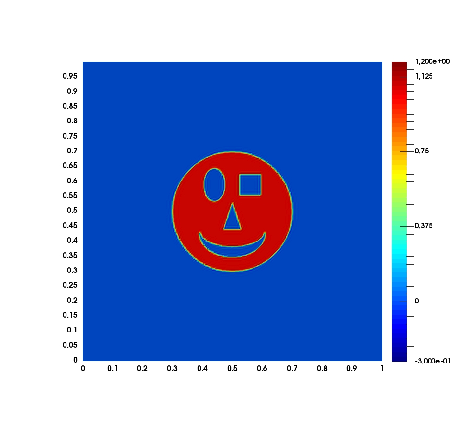
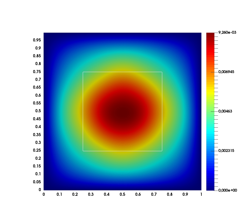
Here, we present numerical results for PAT with the preconditioning method described above using simulated data. The ground truth, the smiley, is represent in Figure 2. It is constructed to be a second order spline with $8$ refinements, that is an element of $S_{2,8}((0,1)^{2})$.

Figure 2: Ground truth $u\in S_{2,8}((0,1)^{2})$.

We used simulated measurement data $z_{d}$, which is obtained by numerically solving the wave equation with the ground truth with the Galerkin method in space and a finite difference method in time, with time step $h_{t}=T/2^{10}$, where $T=\frac{1}{4}$.

For solving the inverse problem of PAT we discretize the augmented optimality system on the space

$$Y_{h}:=S_{2,6}(0,T)\otimes S_{2,6}((0,1)^{2})\cap H^{1}_{0}((0,1)^{2})$$

and $\Lambda_{h}$ according to Equation 4.4. It is obvious that since we make only $6$ refinements, the ground truth cannot be recovered accurately.

The observation surface is again $\Gamma=\partial\Omega_{s}$ and the resulting preconditioned linear system of equations

$$\begin{pmatrix}P_{Y_{\alpha,\rho,h}}^{-1}&0\\ 0&P_{\Lambda_{h}}^{-1}\end{pmatrix}\begin{pmatrix}A_{\alpha,\rho,h}&B_{h}^{\prime}\\ B_{h}&0\end{pmatrix}\begin{pmatrix}y_{h}\\ \lambda_{h}\end{pmatrix}=\begin{pmatrix}P_{Y_{\alpha,\rho,h}}^{-1}&0\\ 0&P_{\Lambda_{h}}^{-1}\end{pmatrix}\begin{pmatrix}l_{h}\\ 0\end{pmatrix}$$

is solved using the MINRES method. This is done by using sparse direct solvers for the sub-systems with the matrices $P_{Y_{\alpha,\rho,h}}=A_{\alpha,\rho,h}$ and $P_{\Lambda_{h}}$. This is currently the bottle neck of the numerical procedure as the direct inversion of such matrices requires a lot of memory, which limits us for instance to a maximum of $\ell=6$ uniform refinements.

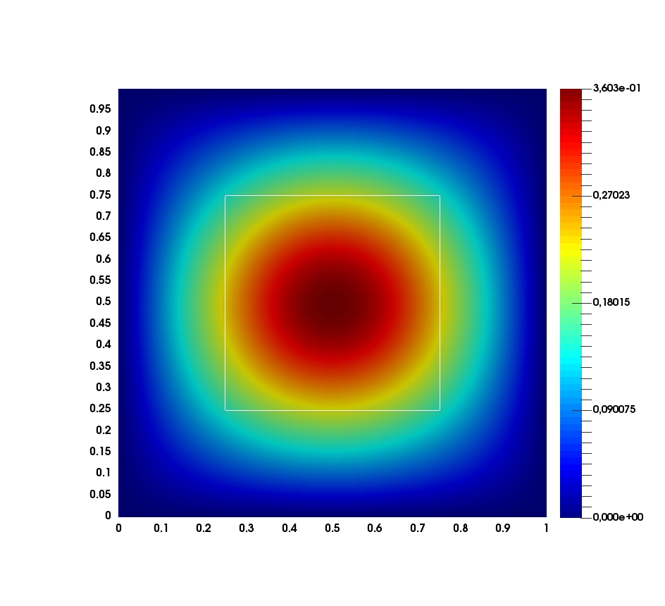
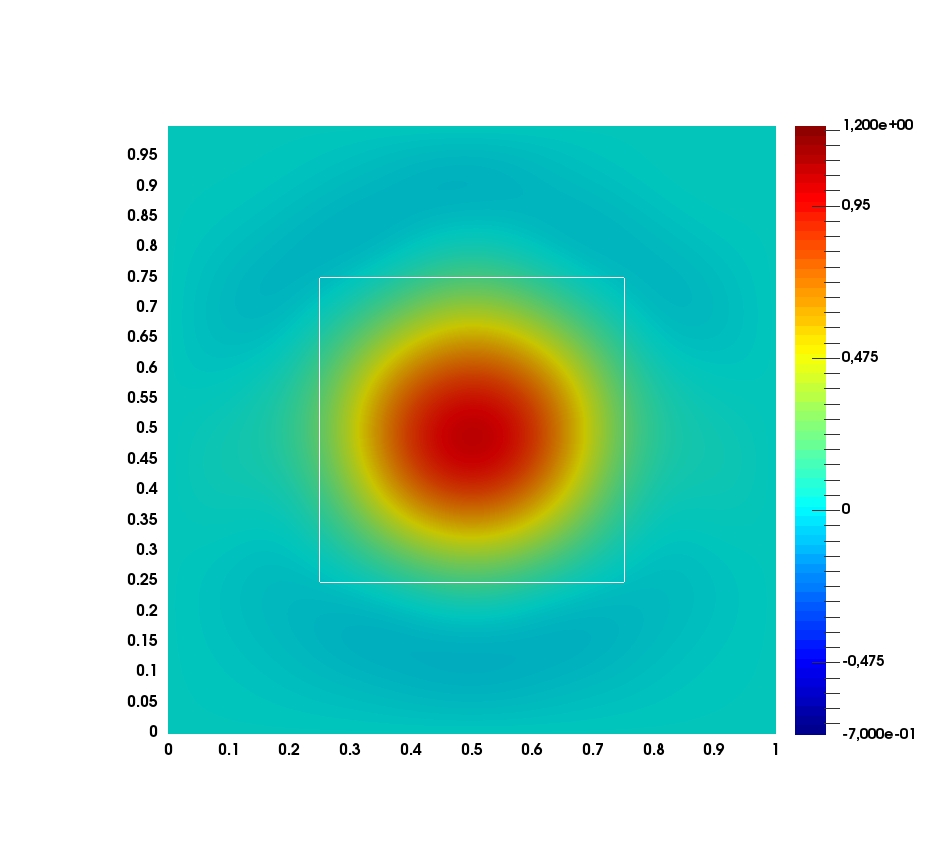
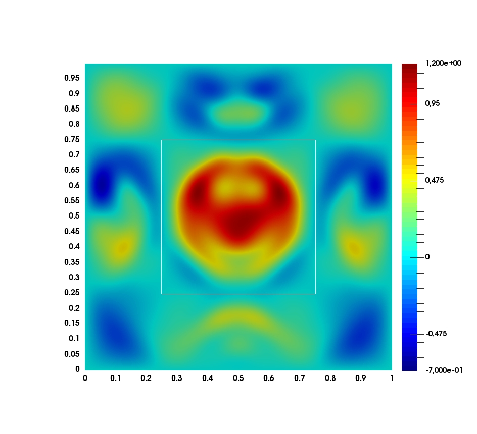
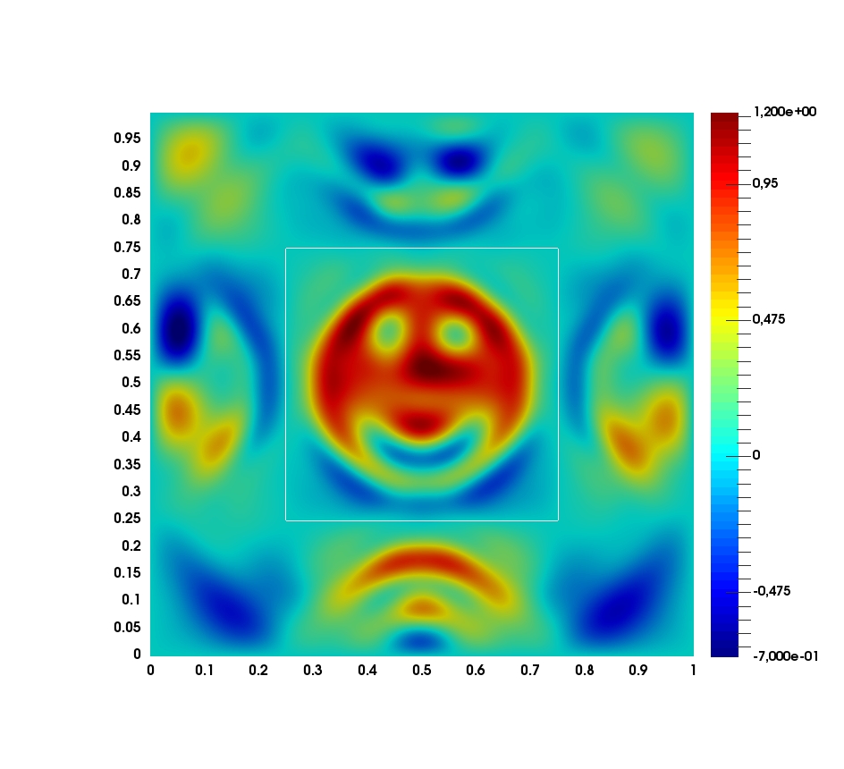
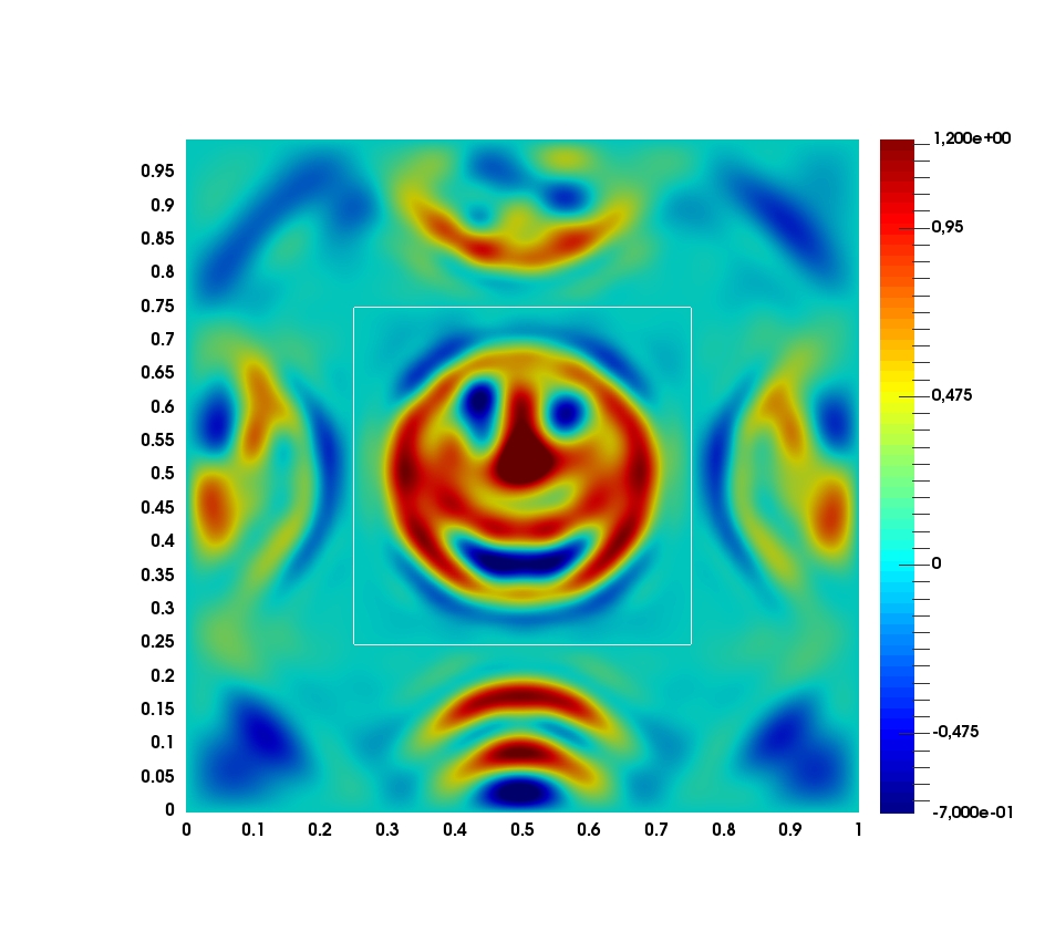
Figure 4 shows the reconstruction for $\alpha=1.0$ and $\rho=1.0$. In Figure 4 we reduced $\alpha$ to $10^{-7}$ while $\rho$ stays the same. Both reconstructions do not resemble the ground truth. For obtaining the results shown in Figure 6, Figure 6, Figure 8 and Figure 8 we reduce $\rho$ to $10^{-2}$, $10^{-5}$, $10^{-6}$ and $10^{-7}$, respectively. We see from these figures that the value $\rho$ significantly effects the recovered image. Smaller values of $\rho$ give a better recovery, however, too small values of $\rho$ yield instabilities which can be observed in Figure 8.

Figure 3: Recovered image: $\alpha=1.0$ and $\rho=1.0$.

Figure 4: Recovered image: $\alpha=10^{-7}$ and $\rho=1.0$.

Figure 5: Recovered image: $\alpha=10^{-7}$ and $\rho=10^{-2}$.

Figure 6: Recovered image: $\alpha=10^{-7}$ and $\rho=10^{-5}$.

Figure 7: Recovered image: $\alpha=10^{-7}$ and $\rho=10^{-6}$.

Figure 8: Recovered image: $\alpha=10^{-7}$ and $\rho=10^{-7}$.

5.3. Discussion regarding the augmented parameter $\rho$

In Subsection 4.2 we presented a stable discretization scheme based on an augmented Lagrangian stabilization and a particular choice of $\Lambda_{h}$. The discrete preconditioner $\mathcal{P}_{\alpha,\rho,h}$ from Subsection 4.2 is not robust with respect to $\rho$, see Subsection 4.2. The iteration number for the preconditioned discretized augmented system $\mathcal{P}_{\alpha,\rho,h}^{-1}\mathcal{A}_{\alpha,\rho,h}$ increases as $\rho$ goes to zero, however a small $\rho$ is needed to recover the desired image, as shown in the figures.

References

• [1] K. Birner and M. Kapl “The space of C1-smooth isogeometric spline functions on trilinearly parameterized volumetric two-patch domains” In Comput. Aided Geom. Design 70, 2019, pp. 16–30 DOI: 10.1016/j.cagd.2019.03.002
• [2] D. Boffi, F. Brezzi and M. Fortin “Mixed Finite Element Methods and Applications” 44, Springer Series in Computational Mathematics Springer Berlin Heidelberg, 2013 DOI: 10.1007/978-3-642-36519-5
• [3] M. Cîndea and A. Münch “Inverse problems for linear hyperbolic equations using mixed formulations” In Inverse Problems 31.7, 2015, pp. 075001 DOI: 10.1088/0266-5611/31/7/075001
• [4] M. Cîndea and A. Münch “Simultaneous reconstruction of the solution and the source of hyperbolic equations from boundary measurements: a robust numerical approach” In Inverse Problems 32.11, 2016, pp. 115020 DOI: 10.1088/0266-5611/32/11/115020
• [5] C. Clason and M.. Klibanov “The quasi-reversibility method for thermoacoustic tomography in a heterogeneous medium” In SIAM Journal on Scientific Computing 30.1 SIAM, 2007, pp. 1–23 DOI: 10.1137/06066970X
• [6] B.. Cox and B.. Treeby “Artifact trapping during time reversal photoacoustic imaging for acoustically heterogeneous media” In IEEE Transactions on Medical Imaging 29.2 IEEE, 2010, pp. 387–396
• [7] R. Hiptmair “Operator Preconditioning” In Comput. Math. Appl. 52.5, 2006, pp. 699–706 DOI: 10.1016/j.camwa.2006.10.008
• [8] T.J.R. Hughes, J.A. Cottrell and Y. Bazilevs “Isogeometric analysis: CAD, finite elements, NURBS, exact geometry and mesh refinement” In Comput. Math. Appl. Mech. Eng. 194.39-41, 2005, pp. 4135–4195 DOI: 10.1016/j.cma.2004.10.008
• [9] J.-L. Lions “Optimal Control of Systems Governed by Partial Differential Equations” New York: Springer Verlag, 1971
• [10] J.-L. Lions and E. Magenes “Non-Homogeneous Boundary Value Problems and Applications I” 181, Die Grundlehren der Mathematischen Wissenschaften New York: Springer Verlag, 1972
• [11] K.-A. Mardal and R. Winther “Preconditioning discretizations of systems of partial differential equations” In Numerical Linear Algebra With Applications 18.1, 2010, pp. 1–40 DOI: 10.1002/nla.716
• [12] W. Rudin “Real and Complex Analysis” 2nd edition, 1st edition 1966 New York: McGraw-Hill, 1974
• [13] P. Stefanov and G. Uhlmann “Thermoacoustic tomography with variable sound speed” In Inverse Problems 25.7, 2009, pp. 075011\bibrangessep16
• [14] L.. Veiga, A. Buffa, G. Sangalli and R. Vázquez “Mathematical analysis of variational isogeometric methods” In Mathematical Models & Methods in Applied Sciences 23, 2014, pp. 157–287 DOI: 10.1017/S096249291400004X
• [15] “Photoacoustic Imaging and Spectroscopy”, Optical Science and Engineering Boca Raton: CRC Press, 2009
• [16] “Biomedical Optics: Principles and Imaging” New York: Wiley-Interscience, 2007