INFaaS: A Model-less and Managed Inference Serving System

Abstract

Despite existing work in machine learning inference serving, ease-of-use and cost efficiency remain challenges at large scales. Developers must manually search through thousands of model/variants – versions of already-trained models that differ in hardware, resource footprints, latencies, costs, and accuracies – to meet the diverse application requirements. Since requirements, query load, and applications themselves evolve over time, these decisions need to be made dynamically for each inference query to avoid excessive costs through naive autoscaling. To avoid navigating through the large and complex trade-off space of model/variants, developers often fix a variant across queries, and replicate it when load increases. However, given the diversity across variants and hardware platforms in the cloud, a lack of understanding of the trade-off space can incur significant costs to developers.

This paper introduces $\mathtt{INFaaS}$, a managed and model-less system for distributed inference serving, where developers simply specify the performance and accuracy requirements for their applications without needing to specify a specific model-variant for each query. $\mathtt{INFaaS}$ generates model/variants, and efficiently navigates the large trade-off space of model/variants on behalf of developers to meet application-specific objectives: (a) for each query, it selects a model, hardware architecture, and model optimizations, (b) it combines VM-level horizontal autoscaling with model-level autoscaling, where multiple, different model-variants are used to serve queries within each machine. By leveraging diverse variants and sharing hardware resources across models, $\mathtt{INFaaS}$ achieves 1.3$\times$ higher throughput, violates latency objectives 1.6$\times$ less often, and saves up to 21.6$\times$ in cost (8.5$\times$ on average) compared to state-of-the-art inference serving systems on AWS EC2.

1 Introduction

The number of applications relying on inference from Machine Learning (ML) models, such as video analytics [82], is already large [47, 65, 45, 14, 73] and expected to keep growing. Facebook, for instance, serves tens-of-trillions of inference queries per day [41, 38]. Consequently, distributed inference dominates ML production costs: on AWS, inference accounts for over 90% of ML infrastructure cost [16].

Inference serving is user-facing. Typically, an ML lifecycle has two distinct phases – training and inference. The training phase is usually characterized by long-running hyperparameter searches, dedicated hardware resource usage, and no completion deadlines. In the inference phase, trained models can be queried by various end-user applications. Being user-facing, inference serving requires cost-effective systems that render predictions with latency constraints while handling unpredictable and bursty request arrivals.

Application	Accuracy	Latency	Cost
Social Media	High	Medium	Low
Visual Guidance	High	Low	High
Intruder Detection	Low	Low	Low

Table 1: Applications querying a face recognition model with diverse requirements.

Inference serving systems face a number of challenges [60, 67] due to the following factors.
(a) Diverse application requirements: Applications issue queries that differ in latency, cost, accuracy, and even privacy [59] requirements [43, 40, 67]. Table 1 shows the same face recognition model queried by multiple applications with different requirements. Some applications, such as intruder detection, require inference in realtime but can tolerate lower accuracy. Others, such as tagging faces on social media, may prefer accuracy over latency.
(b) Heterogeneous execution environments: Leveraging heterogeneous hardware resources (e.g., different generations of CPUs, GPUs, and accelerators like TPU [48] or AWS Inferentia [18]) helps meet the diverse needs of applications and the dynamic changes in the workload; however, it is non-trivial to manage and scale heterogeneous resources [38].
(c) Diverse model/variants: Methods, such as layer fusion or quantization [22, 3, 15], produce versions of the same model, model/variants, that may differ in inference latency, memory footprint, and accuracy.

Together, these factors create a large search space. For instance, from 21 already-trained image classification models, we generated 166 model/variants, by (i) applying model graph optimizers, such as TensorRT [3], (ii) optimizing for different batch sizes, and (iii) changing underlying hardware resources, such as CPUs, GPUs, and Inferentia. These variants vary across many dimensions: the accuracies range from 56.6% to 82.5% (1.46$\times$), the model loading latencies range from 590ms to 11s (18.7$\times$), and the inference latencies for a single query range from 1.5ms to 5.7s (3,700$\times$). Their computational requirements range from 0.48 to 24 GFLOPS (50$\times$) [67], and the cost of hardware these variants incur [17] ranges from $0.096/hr for 2 vCPUs to $3.06/hr for a V100 GPU (32$\times$). As new inference accelerators are introduced and new optimization techniques emerge, the number of model-variants will only grow.

This large search space makes it hard for developers to manually match the requirements of each inference query to decisions about selecting the right model and model optimizations, suitable hardware platforms, and auto-scaling configurations. The decision complexity is further exacerbated when the load varies, applications evolve, and the availability of hardware resources (GPUs, ASICs) changes. Unlike long-running batch data analytics or ML training jobs [35, 58, 8, 74, 25] that can be right-sized during or across subsequent executions, the dynamic nature of distributed inference serving makes it infeasible to select model/variants statically.

Our key insight is that the large diversity of model/variants is not a nuisance but an opportunity: it can allow us to meet the diverse and varying performance, cost, and accuracy requirements of applications, in the face of varying load and hardware resource availability, if only we are able to select and deploy the right model-variant effectively for each query. However, given the complexity of this search space, existing systems, including Clipper [24], TensorFlow Serving [5], AWS SageMaker [11], and others [6, 34, 1, 81], ignore the opportunity. These systems tightly couple a model to a hardware resource and use statically-defined resource management policies. These existing systems require developers to select model/variants, batch sizes, instance/hardware types, and autoscaling configurations, for meeting requirements of each query. If these decisions are made without understanding the trade-offs offered by the variants, the impact could be significant (note the wide cost, performance, and accuracy ranges spanned by the variants). We argue that in addition to traditional autoscaling, distributed inference serving systems should navigate this search space of model/variants on behalf of developers, and automatically manage model/variants and heterogeneous resources to meet the requirements of inference-driven applications. Surprisingly, as we also noted in [60], no existing inference serving system does that.

To this end, we built $\mathtt{INFaaS}$ (INFerence-as-a-Service), a model-less and managed system for distributed inference serving. $\mathtt{INFaaS}$ introduces a model-less interface where after registering trained models, developers do not need to generate, select, or manage the model/variants for their applications. Instead, for each inference query they specify only the high-level performance, cost, or accuracy requirements. $\mathtt{INFaaS}$ generates model/variants of the registered models, and navigates the large space to select a model/variant and automatically switch between differently optimized model-variants to best meet the goals of each query. $\mathtt{INFaaS}$ is managed, because it automates resource provisioning for model/variants and schedules queries across a heterogeneous cluster.

To realize this, $\mathtt{INFaaS}$ generates model/variants and their performance-cost profiles on different hardware platforms. $\mathtt{INFaaS}$ tracks the dynamic status of variants (e.g., overloaded or interfered) using a state machine, to efficiently select the right variant for each query to meet the application requirements. Finally, $\mathtt{INFaaS}$ combines VM-level (horizontal scaling) and model-level autoscaling to dynamically react to the changing application requirements and request patterns. Given the large and complex search space of model/variants, we formulate an integer linear program (ILP) for our model-level autoscaling that finds the most cost-effective combination of model/variants, to meet the goals for queries in large scale inference serving.

Using query patterns derived from real-world applications and traces, we evaluate $\mathtt{INFaaS}$ against existing inference serving systems, including Clipper [24] and SageMaker [11], with 175 variants generated from 22 model architectures, on AWS. Compared to Clipper, $\mathtt{INFaaS}$’ ability to select suitable model/variants, leverage heterogeneous hardware (CPU, GPU, Inferentia), and share hardware resources across models and applications enables it to save 1.23$\times$ in cost, violate latency objectives 1.6$\times$ less often, and improve resource utilization by 2.8$\times$. At low load, $\mathtt{INFaaS}$ saves cost by 21.6$\times$ compared to Clipper, and 21.3$\times$ compared to SageMaker.

2 Challenges

2.1 Selecting the right model/variant

A model/variant is a version of a model defined by the following aspects: (a) model architecture (e.g., ResNet50, VGG16), (b) programming framework, (e.g., TensorFlow, PyTorch, Caffe2, MXNet), (c) model graph optimizers (e.g., TensorRT, Neuron, TVM, XLA [78]), (d) hyperparameters (e.g., optimizing for batch size of 1, 4, 8, or 16), and (e) hardware platforms (e.g., Haswell or Skylake CPUs, V100 or T4 GPUs, FPGA, and accelerators, such as Inferentia [18], TPU [48], Catapult [31], NPU [7]). Based on the 21 image classification models and the available hardware on AWS EC2 [9], we estimate that the total number of possible model/variants would be 4,032. The performance, cost, and accuracy trade-off space offered by these variants is large [67, 19]. As new inference accelerators are introduced and new optimization techniques emerge, the number of model/variants will only grow.

Existing inference serving systems require developers to identify the model/variant that can meet diverse performance, accuracy, and cost requirements of applications. However, generating and leveraging these variants requires a substantial understanding of the frameworks, model graph optimizers, and characteristics of hardware architectures, thus limiting the variants an application developer can leverage. As shown in Table 1, one can use the same face recognition model for several applications, but selecting the appropriate model/variant depends on the requirements of an application [67].

We argue that inference serving systems should automatically and efficiently select a model/variant for each query on behalf of developers to align with application requirements.

2.2 Reducing cost as load varies

Variant (hardware, framework)	Lat. (ms)	Req/s	Cost ($/s)
A (4 CPUs, TensorFlow)	200	5	1
B (1 Inferentia core, Neuron)	20	100	3
C (1 V100 GPU, TensorRT)	15	800	16

Table 2: Latency, saturation throughput, and normalized cost (based on AWS pricing) for three ResNet50 variants.

QPS	SLO (ms)	#Var. A	#Var. B	#Var. C	Cost ($/s)
10	300	2	0	0	2
10	50	0	1	0	3
1000	300	0	2	1	22

Table 3: Cheapest configuration (in #instances) of variants from Table 2 to meet the QPS and SLO; last column shows total cost.

Query patterns and service level objectives (SLOs) of applications, such as real-time translation and video analytics, can vary unpredictably [41, 50, 82]. Provisioning for peak demand leads to high cost, hence distributed inference serving systems need to dynamically respond to changes. Traditional autoscaling focuses on horizontal virtual machine replication (VM-scaling), adding or removing worker machines [32, 36]. Since inference serving is embarrassingly parallel, increasing the number of workers results in proportional increases in throughput and cost. However, relying only on worker replication may incur significant latency, as new machines must be spawned.

Autoscalers used by existing inference serving systems [11, 36, 34] replicate a statically-fixed (developer-specified) model/variant for all the queries of an application. This is insufficient because: (a) the right variant may change with load (e.g., a CPU variant may be more suitable at low QPS to meet the cost SLOs) and (b) the hardware resources needed to replicate the same variant may not always be available (e.g., shortage of GPU instances at some point).

In addition to using VM-scaling and replication-based model-scaling, we introduce model-level vertical scaling, where we switch to a differently optimized variant as load changes. The challenge is to identify which variant to scale to given available hardware resources and query requirements. Consider the example shown in Table 2 with three ResNet50 variants. Each variant runs on a different hardware resource and differs in latency, saturation throughput, and cost. In Table 3, we present three input loads and SLO requirements, with the goal of scaling to the most cost-effective combination of variants. In the first case (QPS = 10 and SLO = 300ms), though all variants can meet the QPS and SLO, using two instances of Variant A is the cheapest choice (8$\times$ cheaper than using Variant C). In the second case, the load remains unchanged, but due to the stricter SLO, Variant B becomes the cheapest choice (5.3$\times$ cheaper than using Variant C). In the third case, the combination of two instances of Variant B and one of Variant C is the cheapest. This configuration is 1.45$\times$ cheaper than using two instances of Variant C (next cheapest configuration), and 9$\times$ cheaper than using 200 instances of Variant A (the most expensive configuration). Deciding the best configuration becomes more challenging as the number of variants increases and resource availability changes.

2.3 Improving utilization at low load

For predictable performance, one may serve each model/variant on a dedicated machine to exclusively access hardware resources. But, this often results in underutilized resources and cost-inefficiency, especially at low load. Instead, the serving systems should support multi-tenancy by sharing resources across applications and models, thereby improving utilization and the overall cost. Recent work [77, 35] has shown the benefits of sharing GPUs for deep-learning training jobs. ML inference jobs are typically less demanding for compute and memory resources than the training jobs, making inference jobs ideal for sharing GPUs and other accelerators [79, 44].

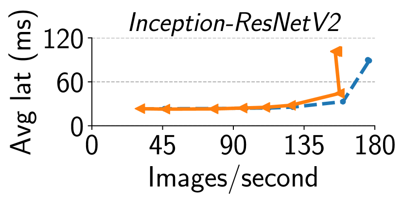
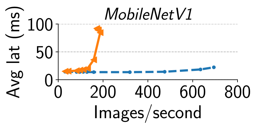
Figure 1: Impact of co-locating Inception-ResNetV2 and MobileNetV1 on a V100 GPU. Both variants are TensorRT, batch-1, FP16. Graphs show average latency and throughput for each model running alone vs sharing, subjected to the same (QPS).

However, how to share accelerators across multiple tenants while maintaining predictable performance is not obvious. Figure 1 shows the result of co-locating a large (Inception-ResNetV2) and a small (MobileNetV1) model on a GPU. At low load, sharing a GPU does not affect the performance of either model. At higher load, this co-location heavily impacts the performance of the small model, while the large model remains unaffected. The point when co-location starts affecting the performance varies across models, and depends on both the load and the hardware architecture.

An additional opportunity to improve resource utilization is to multiplex resources for online (realtime) and offline (batched) inference queries. Typical offline jobs, such as historical data analysis [64] and image labeling [46], process a large number of queries and are latency tolerant (about minutes to hours). Thus, during periods of low or medium online load, offline and online jobs can run on the same machine. The trade-off lies in maximizing the resources used by offline jobs while minimizing the interference to online jobs [57].

3 INFaaS

Design principles.

We design $\mathtt{INFaaS}$ based on the following guidelines. First, $\mathtt{INFaaS}$ should support a declarative API: Developers should not need to specify the model, model optimizations, suitable hardware platforms, or autoscaling configurations; they should only focus on high-level performance, cost, or accuracy requirements. Across queries, the most suitable variant may differ; moreover, the best variant for the same query can be different based on the load and the status of variants and resources. Thus, the second desirable property is that the system should automatically and efficiently select a model/variant, while considering the dynamic state of the model/variants and the hardware resources, for (a) serving each query, and (b) deciding how to scale in reaction to changing application load. Third, to improve resource utilization, the system should share hardware resources across model/variants and applications, without violating performance/cost constraints. Finally, the system design should be modular and extensible to allow new model/variant selection policies. By following these design principles, we naturally address the challenges raised in Section 2.

Functionality.

$\mathtt{INFaaS}$ generates new model/variants from the models registered by developers, and stores them in a repository (Section 3.2). These variants are optimized along different dimensions using model graph optimizers such as Neuron and TensorRT. For each inference query, $\mathtt{INFaaS}$ automatically selects a model/variant to satisfy its performance, cost, and accuracy objectives (Section 4.1). $\mathtt{INFaaS}$’ autoscaler combines VM-level autoscaling with model-level horizontal and vertical autoscaling to meet application performance and cost requirements while improving utilization of resources (Section 4.2). $\mathtt{INFaaS}$ introduces model-vertical autoscaling that, through model selection, upgrades or downgrades to a differently optimized model-variant by leveraging the diversity of model/variants (Section 4.2.1). $\mathtt{INFaaS}$ efficiently maintains static and dynamic profiles of model/variants and hardware resources to support low latencies for selecting and scaling model/variants (Sections 3.2 and 4). Finally, $\mathtt{INFaaS}$ features the model/variant selection policy described in Section 4, but allows developers to extend and customize it.

API	Parameters
register_model	modelName, modelBinary, valSet, appID
online_query	input(s), appID, latency, accuracy
online_query	input(s), modelName
offline_query	inputPath, outputPath, appID, accuracy
offline_query	inputPath, outputPath, modelName

Table 4: $\mathtt{INFaaS}$’ declarative developer API.

3.1 Model-less interface for inference

Table 4 lists $\mathtt{INFaaS}$’ model-less API.

Model registration.

Developers register one or more models using the register_model API. This API accepts a developer-assigned model identifier (modelName), the model (modelBinary) in serialized format (e.g., a TensorFlow SavedModel or model in ONNX format), and a developer-assigned application identifier (appID). Models for different prediction tasks within the same application (e.g., optical character recognition and language translation) can be registered with separate appIDs. Lines 1-2 in Figure 2 show how a developer registers two models, a ResNet50 and a MobileNet, for an application with appID=detectFaceApp. $\mathtt{INFaaS}$ generates multiple variants from these already trained models. For instance, using ResNet50 alone, $\mathtt{INFaaS}$ can generate about 50 variants by changing the batch size, the hardware, and the model graph optimizer (Section 3.2). Note that $\mathtt{INFaaS}$ is an inference serving system and does not train new models; $\mathtt{INFaaS}$ only generates variants from already-trained models. The register_model API takes a validation dataset (e.g., valSet) as input to calculate the accuracy of the newly generated variants. For each incoming query, $\mathtt{INFaaS}$ automatically selects the right model/variant to meet the specified goals.

Query submission.

Being declarative, $\mathtt{INFaaS}$’ API allows developers to specify high-level goals without needing to specify the variants for their queries. $\mathtt{INFaaS}$’ API allows developers to submit online and offline queries in two ways:

• Specifying application requirements. Developers may submit queries for their application and specify high-level application performance, cost, and accuracy requirements (e.g., Line 3 in Figure 2). $\mathtt{INFaaS}$ then navigates the search space of model/variants for the given application, and selects model/variants and scaling strategies. For instance, for a query with appID=detectFaceApp, $\mathtt{INFaaS}$ searches for a suitable variant of ResNet50 and MobileNet to meet the goal of latency (200ms) and accuracy (above 70%).

• Specifying a registered model. Developers may use this interface to specify the model, modelName, they registered for the corresponding application (e.g., "ResNet50" for detectFaceApp). This interface supports developers who want direct control over the model/variant used. This is the only option offered by existing inference systems. $\mathtt{INFaaS}$ then dynamically manages resources for the specified model/variant based on the observed workload.

⬇

1 register_model("ResNet50",ResNet50.pt,valSet,detectFaceApp)

2 register_model("MobileNet",MobileNet.pt,valSet,detectFaceApp)\end{lstlisting}

3 %

4 \begin{lstlisting}[numbers=none,linewidth=\columnwidth,language=Python,basicstyle=\scriptsize\sffamily\mdseries,numberstyle=\tiny,numbersep=-1em,tabsize=2,aboveskip=0pt,belowskip=0pt]

5 # Developer registered 2 models for the detectFaceApp;

6 # INFaaS generates variants from these two registered models\end{lstlisting}

7 %

8 \begin{lstlisting}[firstnumber=3,linewidth=\columnwidth,language=Python,basicstyle=\scriptsize\sffamily\mdseries,numberstyle=\tiny,numbersep=-1em,tabsize=2,aboveskip=0pt,belowskip=0pt,keywordstyle=\scriptsize\sffamily\mdseries]

9 online_query(input.jpg,detectFaceApp, 200ms, 70%)\end{lstlisting}

10 %

11 \begin{lstlisting}[numbers=none,linewidth=\columnwidth,language=Python,basicstyle=\scriptsize\sffamily\mdseries,numberstyle=\tiny,numbersep=-1em,tabsize=2,aboveskip=0pt,belowskip=0pt]

12 # Developer submitted a query with "input.jpg" as the input

13 # and specified requirements; INFaaS then selects a variant

14 # automatically to meet 200ms latency and accuracy > 70%

Figure 2: Registering models and submitting queries with $\mathtt{INFaaS}$.

INFaaS’ serving workflow for an inference query.

Applications interact with $\mathtt{INFaaS}$ by submitting inference queries through the Front-End, logically hosted at the Controller (see steps marked in Figure 3). The Controller selects a model/variant and dispatches the inference query to a Worker machine. Worker machines further send inference queries to the appropriate Hardware Executors according to the selected model/variant, and reply with inference results to applications. Offline inference queries are served asynchronously; $\mathtt{INFaaS}$ notifies the application when the offline job completes.

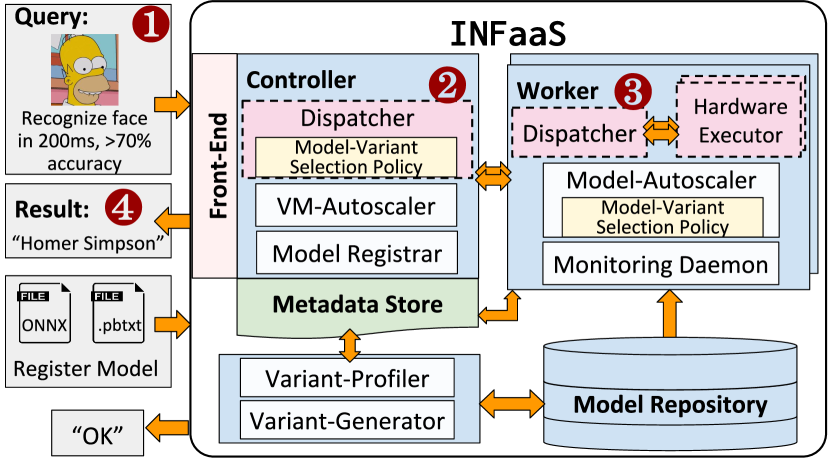
Figure 3: Architecture of $\mathtt{INFaaS}$. Modules in boxes with dashed border are on the critical path of serving queries. All other modules do not impact serving latency. Numbered circles correspond to the typical life-cycle of queries.

3.2 Architecture

We now describe $\mathtt{INFaaS}$’ architecture (Figure 3) in detail.

Controller. The logically-centralized controller receives model registration and inference requests. The controller hosts three modules: (a) The Dispatcher that uses the model/variant selection policy for selecting a variant to serve a query, (b) The VM-Autoscaler that is responsible for scaling the number of workers up and down based on the current load and resource utilization, and (c) The Model Registrar that handles model registration. For fault-tolerance, the controller is replicated using existing techniques [36, 21].

Workers. Worker machines execute inference queries assigned by the controller. Hardware-specific Executor daemons manage the deployment and execution of model/variants. The Dispatcher forwards each query to a specific model/variant instance through the corresponding hardware executor. The Model-Autoscaler detects changes in the load and decides a scaling strategy that either replicates running variants or selects a different variant, within the worker. It uses the model/variant selection policy to select a variant to scale to. The Monitoring Daemon tracks the utilization of machines and variants, and manages resources shared by multiple variants to avoid SLO violations; it also decides when to process or pause offline requests to avoid interference with online serving.

Variant-Generator and Variant-Profiler. From the registered models, the Variant-Generator generates model/variants optimized for different batch sizes, hardware, and hardware-specific parameters (e.g., number of cores on Inferentia) using model graph optimizers, including TensorRT [3] and Neuron [15]. $\mathtt{INFaaS}$ uses the validation set submitted by the developer to calculate the accuracy of the newly generated variants; $\mathtt{INFaaS}$ records this information in the Metadata Store. The Variant-Generator does not train or produce new model architectures: variants are generated only from registered models. To help model/variant selection, the Variant-Profiler conducts one-time profiling for each variant where it measures statistics, such as the loading and inference latencies, and peak memory utilization. These parameters, along with the corresponding appID, accuracy, and maximum supported batch size are recorded in the Metadata Store.

Model-Variant Selection Policy. $\mathtt{INFaaS}$ invokes the model/variant selection policy on two events.
(Case I) On arrival of a query: The controller’s Dispatcher uses the policy to select a variant for each incoming query. This model/variant selection lies on the critical path of serving each query. To reduce the latency of decision-making, we designed an efficient variant search algorithm (Section 4.1).

(Case II) On changes in query load: As the query load changes, the worker’s Model-Autoscaler uses the policy to determine whether to replicate existing variants, or vertically scale to a different variant. The Model-Autoscaler monitors the incoming query load and the current throughput of $\mathtt{INFaaS}$ to detect the need for scaling. If a change is detected, the Model-Autoscaler invokes the policy in the background to select a suitable scaling strategy (Section 4.2).

To allow for other model/variant selection algorithms, we designed $\mathtt{INFaaS}$ to decouple policies from mechanisms [54].

Metadata Store. The Metadata Store enables efficient access to the static and dynamic data about workers and model/variants; this is needed for making model/variant selection and scaling decisions. This data consists of (a) the information about available model architectures and their variants (e.g., accuracy and profiled inference latency), and (b) the resource usage and load statistics of variants and worker machines. The Metadata Store strategically uses data structures to ensure low access latencies ($\sim O(1)$) for efficient decision-making. The Metadata Store runs on the same machine as the controller to reduce access latencies for selecting variants. Implementation and data structure details are described in Section 5.

Model Repository. The Model Repository is a high-capacity persistent storage medium that stores serialized variants that are accessible to workers when needed to serve queries.

4 Selecting and Scaling Model-Variants

$\mathtt{INFaaS}$ uses the model/variant selection policy in two cases: (I) On arrival of a query: $\mathtt{INFaaS}$’ controller needs to select a variant for each query to meet an application’s high-level requirements (Section 4.1). This invocation of the selection policy lies on the critical path of inference serving. (II) On changes in query load: As the query load changes, $\mathtt{INFaaS}$’ workers must decide whether to switch to a differently optimized variant (Section 4.2). The worker invokes the selection policy off the critical path. $\mathtt{INFaaS}$ provides an internal API, getVariant, for invoking model-variant selection policy.

In both cases, $\mathtt{INFaaS}$ needs to consider both the static and dynamic states of variants and available resources. Only considering statically-profiled metadata is insufficient, since the following aspects can significantly impact the observed performance and cost: a selected variant (a) may not be loaded, hence we need to consider its loading latency, (b) may be already loaded but serving at its peak throughput, (c) may be already loaded but experiencing resource contention from co-located inference jobs, and (d) may not be loaded due to lack of resources required for that specific variant. We next describe how $\mathtt{INFaaS}$ tracks the dynamic state of model/variants, and then describe the policy used in the two cases.

State machine for the lifecycle of model/variants. To track the dynamic state of each model/variant instance per-application, $\mathtt{INFaaS}$ uses a state machine (shown in Figure 4). All the registered and generated model/variants start in the Inactive state: they are not loaded on any worker. Once a variant instance is loaded, it transitions to the Active state. These variant instances are serving less than their peak throughput, tracked by the worker’s monitoring daemons. Variant instances enter the Overloaded state when they serve at their peak throughput. Finally, variant instances in the Interfered state are not overloaded but are still experiencing higher inference latencies than the profiled values. Interference occurs when co-located variants contend over shared resources (e.g., caches, memory bandwidth, or hardware threads).

Maintaining the state machine.

The state machine for each model/variant instance is maintained by the worker’s monitoring daemons and is organized in the Metadata Store for fast access. This enables $\mathtt{INFaaS}$’ Dispatcher to use the model/variant selection policy for serving queries on the order of hundreds of $\mu$s to ms (assessed further in Section 6.4). State machine implementation details are described in Section 5.

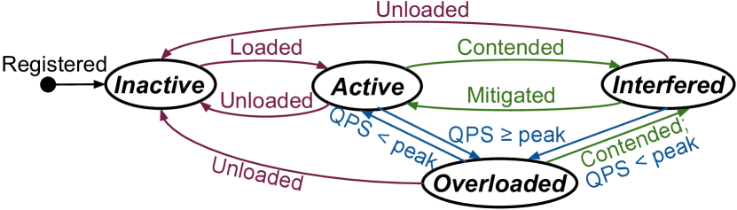
Figure 4: State machine capturing the dynamically changing status of model/variants.

4.1 Case I: On arrival of a query

When a query arrives, $\mathtt{INFaaS}$’ Dispatcher invokes the getVariant method of model/variant selection policy to choose a variant. For this case, the input to getVariant is the query’s requirements, and the output is the variant and worker to serve the query. getVariant first checks whether any variants in the Active state match the query’s requirements. Variants in Active state do not incur a loading latency. If such a variant is found, $\mathtt{INFaaS}$ dispatches the query to the least-loaded worker running the variant instance. Otherwise, $\mathtt{INFaaS}$ considers variants in the Inactive state: getVariant first enquires the Metadata Store and retrieves the variant with the lowest combined loading and inference latency that matches the query’s requirements. If such a variant is found, $\mathtt{INFaaS}$ sends the query to the worker with the lowest utilization on the variant’s target hardware. Otherwise, since no registered or generated variant can meet the developer’s requirements, $\mathtt{INFaaS}$ suggests a variant that can achieve the closest target accuracy and/or latency. We assess the efficiency of this policy over brute-force search in Section 6.4.

Mitigating performance degradation.

For better resource utilization, $\mathtt{INFaaS}$ co-locates variants on hardware resources; as a result, they may interfere and cause SLO violations. To prevent such violations, $\mathtt{INFaaS}$ avoids selecting variants that are in the Interfered or Overloaded state. For interfered variants, $\mathtt{INFaaS}$ triggers a mitigation process in the background to avoid affecting the performance of online serving. If there are idle resources available on the same worker, this mitigation process migrates the variant in the Interfered state to the available resources (e.g., a different set of cores). This avoids the need to fetch a variant from the model repository. If no resources are available for loading the variant on the worker, the worker asks the controller’s Dispatcher to place the variant on the least-loaded worker. For variants in the Overloaded state, $\mathtt{INFaaS}$’ Model-Autoscaler assesses whether it is more cost-effective to scale to a different variant (see Section 4.2.1).

Extensibility.

The state machine and model/variant selection policy are extensible. For instance, getVariant can be extended to prioritize particular variants in the Active state (e.g., prefer least power-hungry variants).

4.2 Case II: On changes in query load

As query load changes, $\mathtt{INFaaS}$ needs to revisit its variant selection decision to check whether a different variant is more cost-efficient. Existing inference serving systems [36, 34, 24, 5, 11] are agnostic to the diversity of model/variants, and only replicate a statically fixed (developer-specified) model/variant for all the queries of an application. However, as discussed in Section 2.2, autoscaling that replicates the same model/variant alone is not enough because: (a) the right model/variant changes with load and (b) the required resources might not be available to replicate a specific variant.

For $\mathtt{INFaaS}$’ autoscaling, in addition to using traditional VM-level, horizontal autoscaling, we introduce model-vertical scaling: change (upgrade or downgrade) to a differently optimized model/variant, thus leveraging the diversity of model/variants. $\mathtt{INFaaS}$’ autoscaling is a joint effort between the workers and the controller. Each worker hosts a Model-Autoscaler that consults with the model/variant selection policy to make model-level autoscaling decisions (Sections 4.2.1, and 4.2.2). The controller hosts a VM-Autoscaler that makes VM-level autoscaling decisions (Section 4.2.3).

4.2.1 Model-Autoscaler at each worker

To react to the changes in query load, $\mathtt{INFaaS}$’ Model-Autoscaler needs to decide the type and number of model/variants to use while minimizing the cost of running the variants. To figure out the type and number of model/variants needed, we formulated the following integer linear program (ILP) that decides a scaling action (replicate, upgrade, or downgrade) for each variant. This ILP minimizes the total cost of scaling actions for all the variants to meet the incoming query load.

Formulation. For an application, the outcome (optimization variable) of our ILP is the optimal scaling action, $\delta_{ij}$, for each model/variant $v_{ij}$, variant $j$ of model architecture $i$. $\delta_{ij}$ is an integer that captures the scaling action as follows: (a) A positive value denotes loading instances of the variant, (b) a negative value denotes unloading instances of this variant, and (c) a value of zero denotes no scaling needed. For a variant $v_{ij}$ that is already loaded, a positive value of $\delta_{ij}$ indicates a replicate action. A positive value of $\delta_{ij}$ for a variant $v_{ij}$ that is not already loaded indicates an upgrade or downgrade action depending on the hardware cost of $v_{ij}$.

The objective function, that our ILP minimizes, is the total cost of all the chosen scaling actions. For a variant $v_{ij}$, this cost for an action $\delta_{ij}$ is the sum of the hardware cost (in $/second), and the loading latency (in seconds) of the variant:

$$\mathrm{Cost}(\delta_{ij})=C_{ij}(\delta_{ij}+\lambda T^{\mathrm{load}}_{ij}\max(\delta_{ij},0))$$

where $C_{ij}$ is the hardware cost (in $/second) for running the variant, $T^{\mathrm{load}}_{ij}$ is the loading latency of the variant, and $\lambda$ (in $\frac{1}{\text{second}}$) is a tunable parameter for the query load unpredictability. Large values of $\lambda$ place more weight on minimizing loading latency to meet SLOs when the query load is unpredictable or spiky. Small values of $\lambda$ place more weight on minimizing the hardware cost when the query load is more stable.

Thus, our objective function, the total cost for all the variants, is: $\sum_{i,j}\text{Cost}(\delta_{ij})$. We impose the following constraints on our ILP:
(1) With the chosen scaling actions, $\mathtt{INFaaS}$ supports the incoming query load.
(2) The newly-loaded instances satisfy applications’ SLOs.
(3) The resources consumed by all variants do not exceed the total system resources.
(4) The number of running instances is non-negative.

We write these constraints formally as:

$$\begin{array}[]{llr}\sum_{i,j}Q_{ij}(N_{ij}+\delta_{ij})\geq L+\texttt{slack}&\text{for all }i,j&(1)\\ T^{\mathrm{inf}}_{ij}\leq S&\text{if }\delta_{ij}>0&(2)\\ \sum_{i,j}R^{\mathrm{type}}_{ij}(N_{ij}+\delta_{ij})\leq R^{\mathrm{type}}_{\mathrm{total}}&\text{for all types}&(3)\\ N_{ij}+\delta_{ij}\geq 0&\text{for all }i,j&(4)\end{array}$$

where (a) $Q_{ij}$: the saturation QPS of variant $v_{ij}$, (b) $N_{ij}$: the number of running instances of variant $v_{ij}$, (c) $L$: the incoming query load, (d) slack: configurable headroom to absorb sudden load spikes, (e) $T^{\mathrm{inf}}_{ij}$: the inference latency of variant $v_{ij}$, (f) $T^{\mathrm{load}}_{ij}$: the loading latency of variant $v_{ij}$, (g) $S$: SLO of the considered application, (h) $R^{\mathrm{type}}_{ij}$: the resource requirements of variant $v_{ij}$, for a resource type (CPU cores, CPU memory, GPU memory, number of Inferentia cores), and (i) $R^{\mathrm{type}}_{\mathrm{total}}$: the total available amount of resources of a type (CPUs, GPUs, Inferentia cores) on the underlying worker machine.

The model/variant selection policy queries the Metadata Store to get the values of these variables.

Practical limitation of the ILP.

Unfortunately, this ILP is NP-complete and hence offers limited practical benefits [33, 75, 55]. Our ILP formulation has to exhaustively search through all the model/variants, track their dynamically changing state, and accurately estimate the QPS each variant can support to find a scaling configuration that can sustain the changed query workload. Gurobi [39] took 23 seconds to find the optimal number of running variant instances across 50 model architectures, and 50 seconds for 100 model architectures. To meet realtime requirements of latency-sensitive applications, $\mathtt{INFaaS}$ must have sub-second response time to query workload changes.

4.2.2 A Greedy Heuristic

The time taken to solve each instance of our ILP makes it impractical to use for $\mathtt{INFaaS}$. Instead, we design a greedy heuristic algorithm that replaces our ILP’s large search space by a subset of model/variants. This pruned search space allows $\mathtt{INFaaS}$ to meet the outlined constraints at sub-second latency. We empirically evaluate the effectiveness of this algorithm in Section 6.2. Each worker machine runs a Model-Autoscaler that, together with the model/variant selection policy, approximates this ILP as follows: (a) Identify whether the constraints are in danger of being violated, (b) Consider two strategies, replicate or upgrade/downgrade, to satisfy the constraints, (c) Compute the objective for each of these scaling actions, and pick the one that minimizes the objective cost function, and (d) Coordinate with the controller to invoke VM-level autoscaling if constraints cannot be satisfied with model-level autoscaling.

Scaling up algorithm: To decide if there is a need to scale (Constraint #1), the Model-Autoscaler estimates the current headroom in capacities of running model/variants, given the profiled values of their saturation throughput, and the current load they are serving. We compute the current load served by a variant using the batch size and number of queries served per second. The load served by a worker is estimated by summing the load served by all running variants. The saturation throughput of all running variants is estimated in a similar manner using the profiled values of model/variants. The Model-Autoscaler then computes the current headroom of a worker as the ratio of the combined saturation throughput and the combined load currently served by the running variants on that worker. $\mathtt{INFaaS}$ maintains a minimum headroom, slack-threshold, on each worker to absorb sudden load spikes. We discuss the value of this tunable parameter in Section 5. When the current headroom is below the required minimum slack-threshold, the Model-Autoscaler concludes that we need to scale, and proceeds to answer the second question: how to scale (replicate or upgrade) to meet the incoming query load.

To decide how to scale, the Model-Autoscaler uses the model/variant selection policy’s getVariant method to select the cheapest option between replication and upgrading. For this case, the input to getVariant is the incoming query load, and the output is the set of scaling actions. The policy first estimates the cost of model-horizontal scaling (replication) by estimating the number of instances of the running variant that would be added to meet the incoming query load (Constraints #1, #4). Secondly, the policy estimates the cost of model-vertical scaling (upgrade), by querying the Metadata Store to select variants of the same model architecture that can meet the SLO (Constraint #2), and support a higher throughput than the currently running variant. The required number of instances for these variants to meet the incoming query load is then estimated. Finally, the model/variant selection policy computes the cost function of our ILP, by using the hardware cost ($/s) and the variant loading latency to decide whether to replicate the running variant, or upgrade to a variant that supports higher throughput. The available resources on the worker limit the number of variant instances it can run (Constraint #3). Thus, if the strategy requires more resources than are available on the current worker (e.g., hardware accelerator), the worker coordinates with the controller to load the variant on a capable worker.

Scaling down algorithm: To decide if and how to scale down (remove replicas or downgrade), the Model-Autoscaler on each worker uses the model/variant selection policy that follows a similar algorithm explained above for scaling up. At regular intervals, this policy checks if the incoming query load can be supported by removing an instance of the running variant, or downgrading to a cheaper variant (optimized for a lower batch size or running on different hardware). The Model-Autoscaler waits for $T_{v}$ time slots before executing the chosen strategy for a variant $v$, to avoid scaling down too quickly. $T_{v}$ is set equal to the loading latency of variant $v$.

4.2.3 VM-Autoscaler at controller

In addition to model-level scaling, $\mathtt{INFaaS}$ also scales the worker machines for deploying variants. Following the mechanisms used in existing systems [20, 42, 24, 11, 34], the VM-Autoscaler decides when to bring a worker up/down:

1. When the utilization of any hardware resource exceeds a configurable threshold across all workers, the VM-Autoscaler adds a new worker with the corresponding hardware resource. We empirically set the threshold to 80%, considering the time to instantiate VMs (20-30 seconds): a lower threshold triggers scaling too quickly and unnecessarily adds workers; a higher value may not scale in time.

2. When variants on a particular hardware platform (e.g., GPU) are in the Interfered state across all workers, the VM-Autoscaler adds a worker with that hardware resource.

3. When more than 80% of workers have Overloaded variants, the VM-Autoscaler starts a new worker.

To improve utilization, $\mathtt{INFaaS}$ dispatches requests to workers using an online bin packing algorithm [70].

5 Implementation

We implemented $\mathtt{INFaaS}$ in about 20K lines of C++ code $\mathtt{INFaaS}$’ API and communication logic between controller and workers are implemented using gRPC in C++ [2]. Developers can interact with $\mathtt{INFaaS}$ by issuing gRPC requests in languages supported by gRPC, such as Python, Go, and Java. $\mathtt{INFaaS}$ uses AWS S3 [10] for its Model Repository. The model/variant selection policy is implemented as an extensible C++ library that is linked into the controller’s Dispatcher and worker’s Model-Autoscaler. getVariant is a virtual method, and can be overridden to add new algorithms.

On the controller machine, the Front-End, Dispatcher, and Model Registrar are threads of the same process for efficient query dispatch. The VM-Autoscaler is a separate process, that polls system status periodically. We swept the polling interval between 0.5-5 seconds at 0.5 second increments (similar to prior work [69, 52]), and arrived at a 2 seconds polling interval. Longer intervals did not scale up fast enough, especially during load spikes, and shorter intervals were too frequent given VM start-up latencies.

On worker machines, the Dispatcher and monitoring daemon run as separate processes. Every two seconds, the monitoring daemon updates compute and memory utilization of the worker, loading, and average inference latencies, along with the current state (as noted in Figure 4) for each variant running on that worker, to the Metadata Store. We deployed custom Docker containers for PyTorch and Inferentia variants, and leveraged Triton Inference Server-19.03 [6] to support TensorRT, Caffe2, and TensorFlow variants on GPU. We used the TensorFlow Serving container for TensorFlow variants on CPU [5]. The Model-Autoscaler’s main thread makes scaling decisions periodically. We swept the same range as the VM-Autoscaler, and arrived at a 1 second polling interval. The interval is shorter than the VM-Autoscaler’s polling interval as model loading latencies are shorter than VM start-up latencies. The main thread also manages a thread pool for asynchronously loading and unloading model/variants. To tune slack-threshold, we explored values between 1.01 and 1.1 [30], and set it to 1.05. In our setup, lower thresholds did not scale variants fast enough to meet load changes, while higher thresholds scaled variants too quickly.

We built the Variant-Generator using TensorRT [3] and Neuron [15]; it is extensible to other similar frameworks [22, 63]. For each variant, the Variant-Profiler records the latency for batch sizes from 1 to 64 (power of two increments). For natural language processing models, we record the latencies of varying sentence lengths for each of these batch sizes.

We built the Metadata Store using Redis [68] and the Redox C++ library [4]. The Metadata Store uses hash maps and sorted sets for fast metadata lookups that constitute the majority of its queries. Per-application, each model/variant instance’s state is encoded as a {variant, worker} pair that can be efficiently queried by the controller and worker.

$\mathtt{INFaaS}$, by design, automates the tedious decision-making aspects of inference serving, thereby allowing an intuitive interface for developers. When needed, we note that $\mathtt{INFaaS}$’ thresholds are configurable, and we used the following values: (a) Resource utilization for pausing offline job (40%), (b) resource utilization for VM-Autoscaler’s scale up action (80%), and (c) Model-Autoscaler’s slack-threshold (1.05).

6 Evaluation

We first compare $\mathtt{INFaaS}$ with all of its optimizations and features to existing systems (Section 6.1). To further demonstrate the effectiveness of $\mathtt{INFaaS}$’ design decisions and optimizations, we evaluate its individual aspects: model/variant selection, scaling (Section 6.2), and SLO-aware resource sharing (Section 6.3). Finally, we quantify the overheads of $\mathtt{INFaaS}$’ decision-making (Section 6.4). We begin by describing the experimental setup common across all experiments, the baselines, the model/variants, and the workloads.

Features	Clipper, TFS, TIS	SageMaker, AI Platform	$\mathtt{INFaaS}$
Model-less abstraction	No	No	Yes
Variant selection	Static	Static	Dynamic
VM-autoscaling	No	Yes	Yes
Model-horizontal scaling	No	Yes	Yes
Model-vertical scaling	No	No	Yes
SLO-aware resource sharing	No	No	Yes

Table 5: Comparison between $\mathtt{INFaaS}$ and the baselines.

Experimental setup. We deployed $\mathtt{INFaaS}$ on a heterogeneous cluster of AWS EC2 [9] instances. We hosted the controller on an m5.2xlarge instance (8 vCPUs, 32GiB DRAM), and workers on inf1.2xlarge (8 vCPUs, 16GiB DRAM, one AWS Inferentia), p3.2xlarge (8 vCPUs, 61GiB DRAM, one NVIDIA V100 GPU), and m5.2xlarge instances. All instances feature Intel Xeon Platinum 8175M CPUs operating at 2.50GHz, Ubuntu 16.04 with 4.4.0 kernel, and up to 10Gbps networking speed.

Baselines. To the best of our knowledge, no existing system provides a model-less interface like $\mathtt{INFaaS}$; state-of-the-art serving systems require developers to specify the variant and hardware. For a fair comparison, we configured $\mathtt{INFaaS}$ to closely resemble the resource management, autoscaling techniques, and APIs of existing systems, including TensorFlow Serving [5] (TFS), Triton Inference Server (TIS) [6], Clipper [24], AWS SageMaker [11] (SM), and Google AI Platform [34]. Specifically, we compared $\mathtt{INFaaS}$ to the following baseline configurations for online query execution:

• $\mathtt{Clipper}^{+}$: Derived from TFS, TIS, and Clipper, this baseline pre-loads model/variants, and requires developers to set a pre-defined number of variant instances. Thus, we set the number of variant instances such that $\mathtt{Clipper}^{+}$ achieves the highest performance given available resources.

• $\mathtt{SM}^{+}$: Derived from SageMaker and AI Platform, this baseline scales each model/variant horizontally, but does not support model-vertical scaling that $\mathtt{INFaaS}$ introduces.

Table 5 lists the differences between baselines and $\mathtt{INFaaS}$. Configuring the baselines with $\mathtt{INFaaS}$ (a) allowed for a fair comparison by removing variabilities in execution environments (e.g., RPC and container technologies), and (b) enabled us to evaluate our design decision individually by giving the baselines access to $\mathtt{INFaaS}$’ features and optimizations, including: support for model graph optimizations, and $\mathtt{INFaaS}$’ detection and mitigation of variant performance degradation.

$\mathtt{Clipper}$ vs $\mathtt{Clipper}^{+}$.

To validate our baseline configurations through $\mathtt{INFaaS}$, we evaluated $\mathtt{Clipper}^{+}$ against the open-source Clipper deployment ($\mathtt{Clipper}$) [23] with its adaptive batching and prediction caching features enabled. We deployed two ResNet50 TensorFlow CPU instances for each. For $\mathtt{Clipper}$, we swept its adaptive batching SLO from 500ms to 10 seconds, and found it achieved its maximum throughput (7 QPS) when setting the SLO to 1 second. For the same SLO, $\mathtt{Clipper}^{+}$ was able to achieve 10 QPS. As prior work has noted [72], $\mathtt{Clipper}$’s adaptive batching is insufficient for maintaining a high QPS, because it relies on an external scheduler to allocate resources for it. Since $\mathtt{Clipper}^{+}$ benefits from $\mathtt{INFaaS}$’ resource allocation and management, variant performance degradation detection and mitigation, and variant optimizations, we use $\mathtt{Clipper}^{+}$ in the place of $\mathtt{Clipper}$ for the remainder of our evaluation.

$\mathtt{SageMaker}$ vs $\mathtt{SM}^{+}$.

We also validated that the latency and throughput of CPU, GPU, and Inferentia variants with $\mathtt{SM}^{+}$ closely match $\mathtt{SageMaker}$, while offering the benefits outlined for $\mathtt{Clipper}^{+}$. Thus, we use $\mathtt{SM}^{+}$ in the place of $\mathtt{SageMaker}$ as our baseline.

Model Family (Task)	#Vars	Model Family (Task)	#Vars
MobileNet (classification)	13	VGG (classification)	30
AlexNet (classification)	9	Inception (classification)	25
DenseNet (classification)	22	NasNet (classification)	6
ResNet (classification)	61	GNMT (translation)	9

Table 6: Model architectures, tasks, and associated variants.

Model/variants. Guided by the MLPerf Inference benchmark [67], we collected a variety of models. Table 6 shows the 8 model families (22 architectures) and the number of associated variants. Our models are pre-trained using Caffe2, TensorFlow, and PyTorch. Our classification models are pre-trained on ImageNet [29]; translation models are pre-trained on the WMT16 [76] English-German dataset. We generated 175 variants in total, differing in the frameworks (Caffe2, TensorFlow, PyTorch), compilers (TensorRT, Neuron), batch sizes (1 to 64), and hardware platforms (CPU, GPU, Inferentia).

Workloads. We evaluated using both synthetic and real-world application query patterns. For synthetic workloads, we used common patterns [28] indicating flat and fluctuating loads, with a Poisson inter-arrival rate [67, 37]. For real-world inference workloads, we used the timing information from a Twitter trace from 2018 collected over a month [13] since there is no publicly available inference serving production traces. Twitter queries are likely passed through hate speech detection models [27] before being posted. Furthermore, as noted in recent work on inference serving [81], this trace resembles real inference workloads with both diurnal patterns and unexpected spikes (consistent with production serving workloads [71]). For each experiment, we randomly selected one day out of the month from the Twitter trace.

6.1 INFaaS with production workload

We now show that through model selection, resource allocation, and autoscaling mechanisms, $\mathtt{INFaaS}$ improves the throughput, cost, utilization, and reduces SLO violations compared to the baselines.

Experimental setup. We mapped the Twitter trace to a range between 10 and 1K QPS for a total of 113,420 batch-1 queries. We used all 22 model architectures. Based on prior work [53], we used a Zipfian distribution for model popularity. We designated 4 model architectures (DenseNet121, ResNet50, VGG16, and InceptionV3) to be popular with 50ms SLOs and share 80% of the load. The rest are cold models with SLO set to 1.5$\times$ the profiled latency of each model’s fastest CPU variant. Baselines statically selected GPU variants for popular models, and CPU variants for the rest; they used 5 CPU and 7 GPU workers. $\mathtt{INFaaS}$ started with 5 CPU, 5 GPU, and 2 Inferentia workers. We computed the worker costs based on AWS EC2 pricing [17].

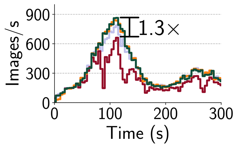
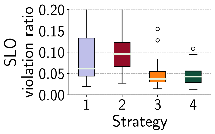
Figure 5: Throughput and SLO violation ratio (# of SLO violations by total # of queries), measured every 4 seconds. Each box shows the median, 25% and 75% quartiles; whiskers extend to the most extreme non-outlier values (1.5$\times$ interquartile range). Circles show the outliers.

Results and discussion. Figure 5 shows that $\mathtt{INFaaS}$ achieved 1.1$\times$ and 1.3$\times$ higher throughput, and 1.63$\times$ and 2.54$\times$ fewer SLO violations compared to $\mathtt{Clipper}^{+}$ and $\mathtt{SM}^{+}$, respectively. $\mathtt{INFaaS}$ scaled models both horizontally and vertically: it upgraded to Inferentia or GPU (higher batch) variants when needed. In reaction to the increased load, $\mathtt{INFaaS}$ added a 3^rd Inferentia worker at 40 seconds. Although $\mathtt{SM}^{+}$ scales variants horizontally, it achieved lower throughput and violated more SLOs due to frequently incurring variant loading penalties and being unable to upgrade variants. By leveraging variants that span heterogeneous hardware (CPU, GPU, Inferentia), $\mathtt{INFaaS}$ achieved 1.23$\times$ lower cost, while keeping SLO violations under 4% on average. $\mathtt{INFaaS}$ also load-balanced requests and mitigated overloaded or interfered variants. This resulted in an average worker utilization of 48.9%, with an average GPU DRAM utilization of 58.6% (5.6$\times$ and 2.8$\times$ higher than $\mathtt{SM}^{+}$ and $\mathtt{Clipper}^{+}$, respectively).

We then added 4 concurrent offline requests to evaluate the efficiency of $\mathtt{INFaaS}$’ resource management. Each offline request contained 500 input images and specified the ResNet50 PyTorch variant. As shown in Figure 5, $\mathtt{INFaaS}$ w/offline maintained similar throughput and SLO violations compared to $\mathtt{INFaaS}$ only serving online requests. Across 3 runs, 756 images on average were processed by offline queries. By dynamically throttling offline requests, $\mathtt{INFaaS}$ guaranteed SLOs for online requests. $\mathtt{INFaaS}$ achieved higher performance (1.3$\times$ higher throughput) and resource utilization (5.6$\times$ higher GPU utilization), and lower SLO violations (2$\times$ lower) and cost (1.23$\times$ lower) compared to the baselines.

6.2 Selecting and scaling model/variants

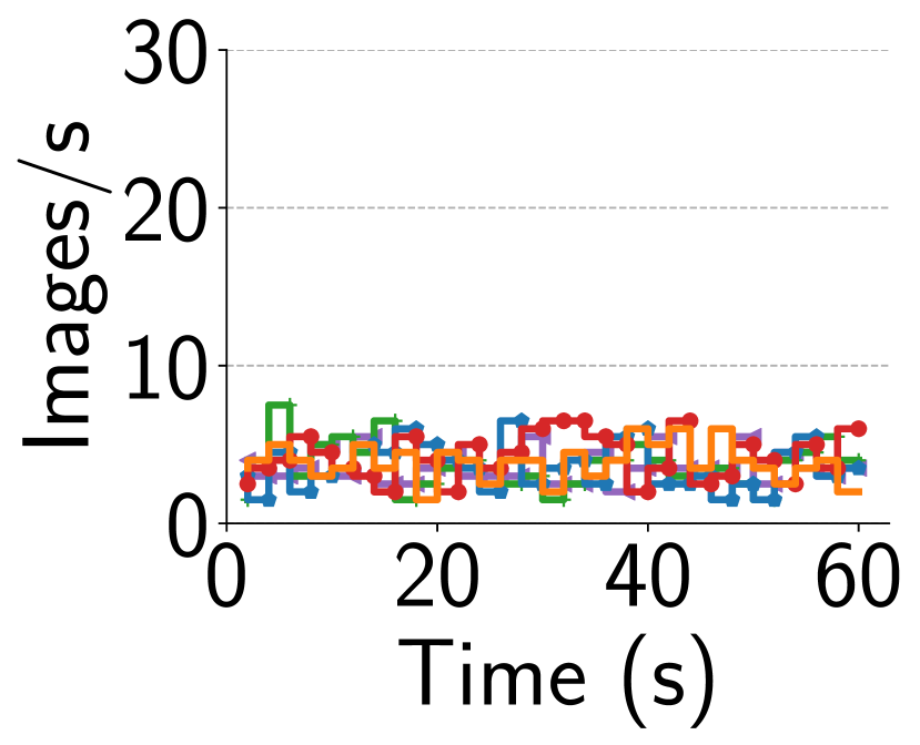
(a) Flat, low load

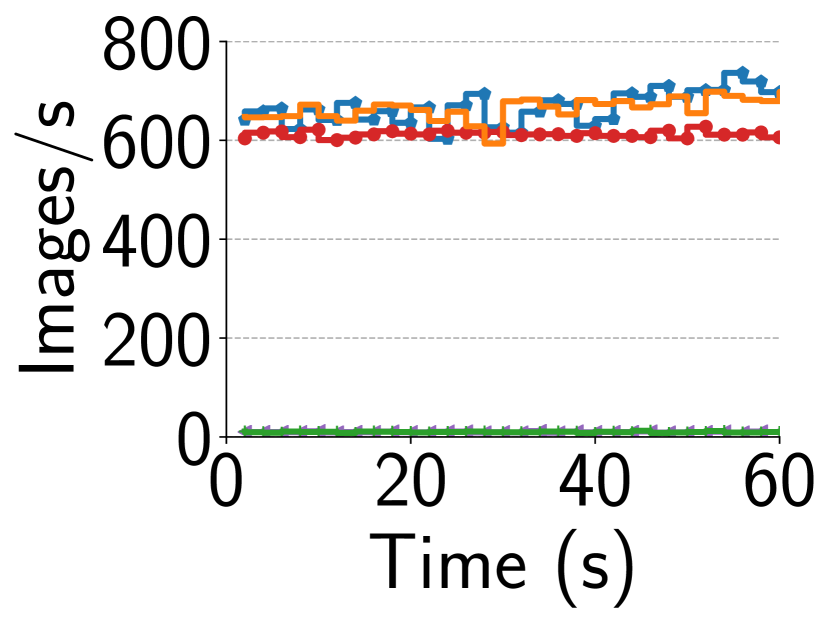
(b) Steady, high load

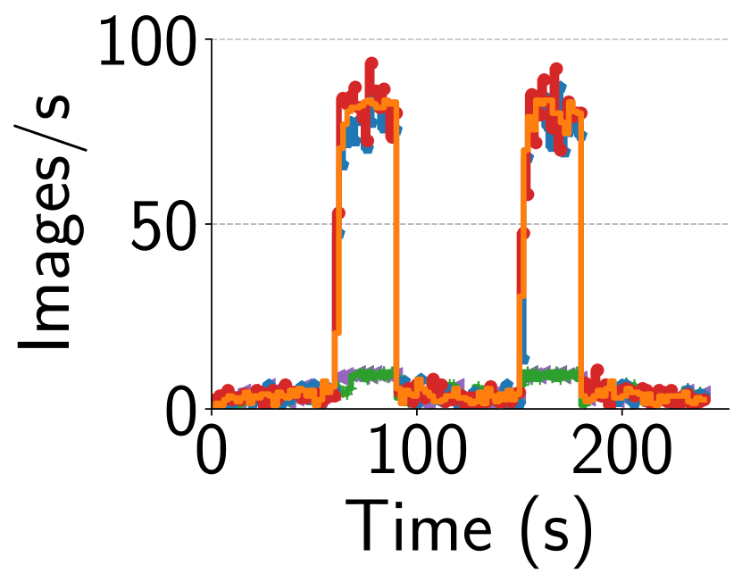
(c) Fluctuating load

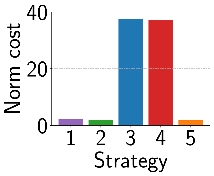
(d) Flat, low load

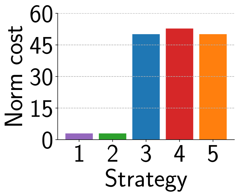
(e) Steady, high load

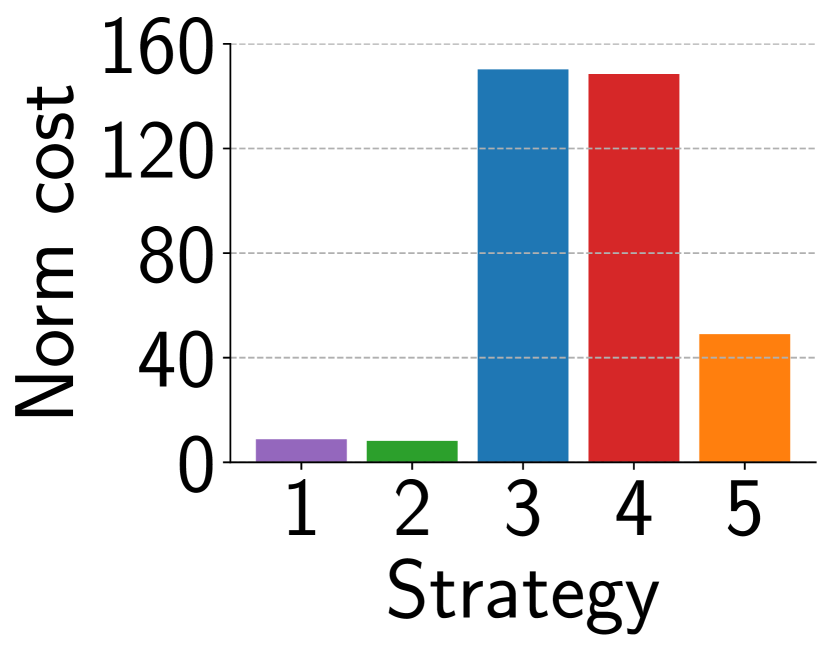
(f) Fluctuating load

Figure 6: Throughput (top) and cost (bottom), with ResNet50 and batch-1 requests. $\mathtt{INFaaS}$ reduced cost and met the load requirement.

Next, we show the efficiency of $\mathtt{INFaaS}$’ model/variant selection policy to select and vertically scale the variants.

Experimental setup. To compare $\mathtt{INFaaS}$ with common configurations developers would choose today, we considered two cases for a model: only GPU variants are used ($\mathtt{Clipper}^{+}_{\mathtt{GPU}}$, $\mathtt{SM}^{+}_{\mathtt{GPU}}$) and only CPU variants are used ($\mathtt{Clipper}^{+}_{\mathtt{CPU}}$, $\mathtt{SM}^{+}_{\mathtt{CPU}}$). We used variants derived from one model architecture, ResNet50, and one worker. $\mathtt{Clipper}^{+}_{\mathtt{CPU}}$ pre-loads and persists 2 instances of the TensorFlow CPU variant. $\mathtt{Clipper}^{+}_{\mathtt{GPU}}$ persists one TensorRT variant optimized for batch size of 8, configured to serve the provided peak load by adaptive batching. $\mathtt{SM}^{+}_{\mathtt{CPU}}$ horizontally scales the CPU variant. $\mathtt{SM}^{+}_{\mathtt{GPU}}$ horizontally scales a batch-1 optimized TensorRT variant (the cheapest GPU variant). We measured throughput every 2 seconds, and calculated the total cost. The cost for a running variant instance is estimated based on AWS EC2 pricing [17], proportional to its memory footprint. We normalize cost to 0.031 per GB/s for CPU, 0.190 per GB/s for Inferentia, and 0.498 per GB/s for GPU.

Workloads. We used three query patterns that are commonly observed in real-world setups [28]: (a) a flat, low load (4 QPS), (b) a steady, high load (slowly increase from 650 to 700 QPS), and (c) a fluctuating load (ranging between 4 and 80 QPS).

Results and discussion. Figures 6(a) and 6(d) show the throughput and total cost, respectively, for $\mathtt{INFaaS}$ and the baselines when serving a flat, low load. While all systems met this low throughput demand, $\mathtt{Clipper}^{+}_{\mathtt{GPU}}$ and $\mathtt{SM}^{+}_{\mathtt{GPU}}$ incurred high costs since they use GPUs. $\mathtt{INFaaS}$ automatically selected CPU variants as they met the demand, thus reducing cost by 21.6$\times$ and 21.3$\times$ compared to $\mathtt{Clipper}^{+}_{\mathtt{GPU}}$ and $\mathtt{SM}^{+}_{\mathtt{GPU}}$, respectively. For a steady, high load (Figures 6(b) and 6(e)), the observed throughput of $\mathtt{Clipper}^{+}_{\mathtt{CPU}}$ and $\mathtt{SM}^{+}_{\mathtt{CPU}}$ (about 10 QPS) was significantly lower than the demand. $\mathtt{INFaaS}$ automatically selected the batch-8 GPU variant, and both $\mathtt{INFaaS}$ and $\mathtt{Clipper}^{+}_{\mathtt{GPU}}$ met the throughput demand. While $\mathtt{SM}^{+}_{\mathtt{GPU}}$ replicated to 2 batch-1 GPU variants to meet the load, it was 5% more expensive than $\mathtt{INFaaS}$ and served 15% fewer QPS. Finally, for a fluctuating load (Figures 6(c) and 6(f)), $\mathtt{INFaaS}$, $\mathtt{Clipper}^{+}_{\mathtt{GPU}}$, and $\mathtt{SM}^{+}_{\mathtt{GPU}}$ met the throughput demand, while both $\mathtt{SM}^{+}_{\mathtt{CPU}}$ and $\mathtt{Clipper}^{+}_{\mathtt{CPU}}$ served only 10 QPS. During low load periods, $\mathtt{INFaaS}$ selected a CPU variant. At load spikes (60-90 and 150-180 seconds), $\mathtt{INFaaS}$ upgraded to an Inferentia batch-1 variant. Hence, on average, $\mathtt{INFaaS}$ was 3$\times$ cheaper than $\mathtt{SM}^{+}_{\mathtt{GPU}}$ and $\mathtt{Clipper}^{+}_{\mathtt{GPU}}$. We found that if $\mathtt{INFaaS}$ were limited to CPU and GPU variants, it would still save 1.7$\times$ cost over both the baselines. Similarly, even if we allowed baselines to use Inferentia, $\mathtt{INFaaS}$ would still save 1.9$\times$ cost because baselines cannot dynamically switch between Inferentia and CPU variants. Thus, leveraging variants optimized for different hardware through model-vertical scaling, $\mathtt{INFaaS}$ is able to adapt to changes in load and query patterns, and improve cost by up to 21.6$\times$ (10$\times$ on average).

6.3 Effectiveness of sharing resources

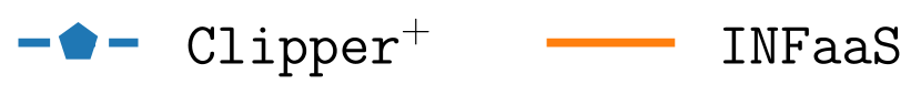
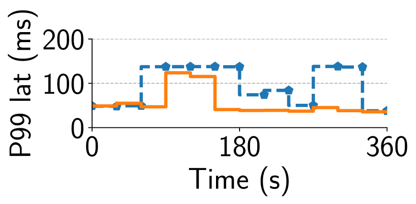
(a) Inception-ResNetV2

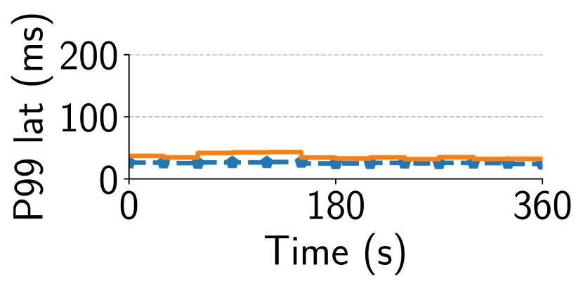
(b) MobileNetV1

(c) Inception-ResNetV2

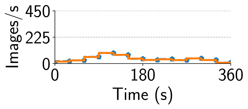
(d) MobileNetV1

Figure 7: Performance of co-locating GPU model/variants when 80% of queries are served by Inception-ResNetV2.

6.3.1 Sharing accelerators

We now show how $\mathtt{INFaaS}$ manages and shares accelerators across models without affecting performance of queries. We found that co-locating models on an Inferentia chip did not cause noticeable interference, since variants can run on separate cores on the chip. Thus, we focus on evaluating GPU sharing. $\mathtt{INFaaS}$ detects when model/variants enter the Overloaded/Interfered state, and either migrates the model to a different GPU, or scales to a new GPU worker if all existing variants on the GPUs are in the Overloaded/Interfered state.

Experimental setup. We used the baseline of $\mathtt{Clipper}^{+}$ with one model persisted on each GPU. Since $\mathtt{Clipper}^{+}$ requires a pre-defined number of workers, we specified 2 GPU workers. For fairness, $\mathtt{INFaaS}$ started from one GPU and was allowed to scale up to 2 GPU workers. As noted in Section 2.3, the load at which sharing of GPUs starts affecting the performance negatively is different across models. We selected two model/variants that diverge in inference latency, throughput, and peak memory: Inception-ResNetV2 (large model) and MobileNetV1 (small model). Both variants are TensorRT-optimized for batch-1. We report throughput and P99 latency, measured every 30 seconds.

Workloads. To show the impact of model popularity on resource sharing, we evaluated a scenario with a popular model serving 80% QPS, and the other serving 20% QPS. We observed similar results with other popularity distributions or different models. We mapped the Twitter trace to a range between 50 and 500 QPS for a total of 75,000 batch-1 queries.

Results and discussion. Figure 7 shows P99 latency and throughput for both models when Inception-ResNetV2 is popular. When Inception-ResNetV2 and MobileNetV1 exceeded their profiled latencies, $\mathtt{INFaaS}$ marked them as interfered around 30 and 50 seconds, respectively. $\mathtt{INFaaS}$ started a new GPU worker ($\sim$30 seconds start-up latency), created an instance of each model on it, and spread the load for both models across the GPUs. The allocated resources for Inception-ResNetV2 with $\mathtt{Clipper}^{+}$ were insufficient and led to a significant latency increase and throughput degradation. Unlike $\mathtt{Clipper}^{+}$, $\mathtt{INFaaS}$ could further mitigate the latency increase by adding more GPU workers (limited to two in this experiment). Moreover, $\mathtt{INFaaS}$ saved 10% cost compared to $\mathtt{Clipper}^{+}$ by (a) bin-packing requests across models to one GPU at low load, and (b) only adding GPUs when contentions were detected.

6.3.2 Co-locating online and offline jobs

In this section, we show using spare resources from online queries for offline jobs allows $\mathtt{INFaaS}$ to improve utilization. To maintain performance for online queries, $\mathtt{INFaaS}$ throttles offline queries when utilization for the underlying worker exceeds a threshold (set to 40%), or the observed latency for online queries exceeds a model/variant’s profiled latency. Lower thresholds would starve offline queries, while higher thresholds would incur severe interference.

Experimental setup. We used one model architecture (ResNet50), one CPU worker, and pre-loaded 2 TensorFlow ResNet50 instances on CPU. Online requests had a 500ms latency SLO, and load fluctuated between 3 to 8 QPS. One offline request to ResNet50 was submitted at the beginning of the experiment, containing 500 input images.

(a) Tail latency for online

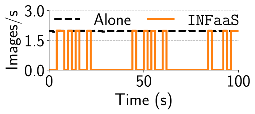
(b) Throughput for offline

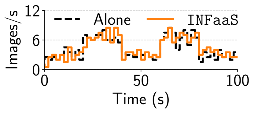
(c) Throughput for online

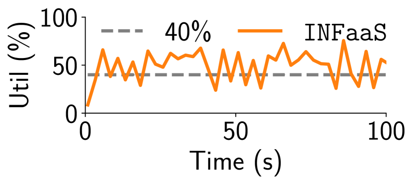
(d) Worker CPU utilization

Figure 8: Performance and utilization of online-offline queries with ResNet50. Alone: Serving either online or offline queries, but not both; $\mathtt{INFaaS}$: Serving both.

Results and discussion. Figures 8(a) to 8(c) contrast the performance of online and offline queries when running alone vs co-located by $\mathtt{INFaaS}$. Figure 8(d) shows the CPU utilization change for $\mathtt{INFaaS}$; the 40% threshold is marked. $\mathtt{INFaaS}$ maintained performance for online requests in both cases by dynamically throttling offline queries. On average, 52 images were processed by offline queries during the co-locating period (0-100 seconds). $\mathtt{INFaaS}$ throttled offline queries for two long periods (Figure 8(b)): 20-40 and 60-80 seconds, due to high online resource utilization (60% – 70%).

6.4 INFaaS’ decision overhead

On the critical path of serving a query, $\mathtt{INFaaS}$ makes the following decisions: (a) selecting a model/variant and (b) selecting a worker. Table 7 shows the median latency of making these decisions for $\mathtt{INFaaS}$ and the speedup over a brute-force search. Each row corresponds to a query specifying (1) a registered model and (2) application requirements. For each query, we show the decision latency when the selected variant was in (a) Inactive, Overloaded, or Interfered state, and (b) Active state. These decisions are made using the model/variant selection policy (Section 4.1).

When the registered model was explicitly specified, $\mathtt{INFaaS}$ incurred low overheads ($\sim$1ms), as it needed to select only a worker. When the application requirements were provided, and the selected variant was not already loaded (State (a)), $\mathtt{INFaaS}$ selected a variant and the least-loaded worker for serving in 3.5ms. Otherwise, when the selected variant was already loaded (State (b)), $\mathtt{INFaaS}$’ decision latency for selecting the variant and a worker was 2.2ms. $\mathtt{INFaaS}$ maintains low overheads across its different query submission modes: up to 44$\times$ (35.5$\times$ on average) faster than a brute-force search.

Query	Variant Picked (Valid Options)	Median Latency in ms (Speedup vs brute-force)
		State (a)	State (b)
resnet50-trt	resnet50-trt (1)	1.0 (N/A)	0.9 (N/A)
appID, >72%, 20ms	inceptionv3-trt (5)	3.5 (27$\times$)	2.2 (44$\times$)

Table 7: Median latency and speedup of making variant and worker selection decisions across 3 runs. State (a): variants are in the Inactive state, Overloaded state, or Interfered state. State (b): variants are in the Active state.

7 Related Work

Inference serving systems. TensorFlow Serving [5] provided one of the first production environments for models trained using the TensorFlow framework. Clipper [24] generalized it to enable the use of different frameworks and application-level SLOs. Pretzel [53] built upon Clipper for optimizing the pipelines of inference serving. SageMaker [11], AI Platform [34], and Azure ML [1] offer developers separate online and offline services that autoscale VMs based on load. Triton Inference Server [6] optimizes GPU inference serving, supports CPU models, but requires static model instance configuration. DeepRecSys [37] statically optimizes batching and hardware selection for recommender systems, but requires developers to specify a variant, manage and scale model resources as the load varies. Tolerance Tiers [40] allows developers to programmatically trade accuracy off for latency. None of these existing systems offer a simple model-less interface, like $\mathtt{INFaaS}$, to navigate the variant search space on developers’ behalf, or dynamically leverage model/variants to meet applications’ diverse requirements.

Model/variant generators. Model graph optimizers [12, 3, 22, 78] perform optimizations, such as quantization and layer fusion, to improve latency and resource usage. However, developers still need to manually create and select variants, and manage the deployed variants. $\mathtt{INFaaS}$ uses these optimizers to create variants that can be used for meeting diverse application requirements, and automates model/variant selection for each query to minimize cost as load and resources vary.

Scaling. Autoscale [32] reviewed scaling techniques and argued for a simple approach that maintains the right amount of slack resources while meeting SLOs. Similarly, $\mathtt{INFaaS}$’ autoscalers maintain headrooms and scale-down counters to cautiously scale resources. MArk [81] proposed SLO-aware model scheduling and scaling by using AWS Lambda to absorb unpredictable load bursts. Existing systems [36, 34, 11, 1] only support VM-level and model-horizontal scaling, while $\mathtt{INFaaS}$ introduces model-vertical scaling that leverages multiple diverse variants.

Sharing accelerators. NVIDIA MPS [61] enabled efficient sharing of GPUs that facilitated initial exploration into sharing GPUs for deep-learning. Existing systems [6, 26, 79, 44] also explored how to share GPUs spatially, temporally, or both. Future NVIDIA GPUs will support MIG [62]: hardware partitions and full isolation. AWS Inferentia supports spatial and temporal sharing via Neuron SDK [15]. $\mathtt{INFaaS}$’ current implementation builds on Triton Inference Server (GPUs) and Neuron SDK (Inferentia), and provides SLO-aware accelerator sharing. $\mathtt{INFaaS}$ can also be extended to leverage other mechanisms for sharing additional hardware resources.

8 Conclusion and Future Work

We presented $\mathtt{INFaaS}$: a model-less and managed system for distributed inference serving. $\mathtt{INFaaS}$’ model-less interface allows application developers to specify high-level performance, cost or accuracy requirements for queries, leaving $\mathtt{INFaaS}$ to select and deploy the model/variant, hardware, and scaling configuration. $\mathtt{INFaaS}$ automatically provisions and manages resources for serving inference queries to meet their high-level goals. We demonstrated that $\mathtt{INFaaS}$’ model/variant selection policy and resource sharing leads to reduced costs, better throughput, and fewer SLO violations compared to state-of-the-art inference serving systems.

Going forward, we plan to explore the challenges of managing reconfigurable hardware architectures, such as FPGAs and CGRAs [80, 51, 66], in a model-less setting, and how they can be utilized to meet diverse application requirements. Secure and privacy-preserving ML is in its nascent stage [59, 56, 49]; we plan to investigate the implications of privacy requirements from applications on model-less inference serving.

Appendix A Model Architectures & Variants

Table 8 shows details of the models we used for evaluating $\mathtt{INFaaS}$. Model architectures within the same model family (corresponding to Table 6) are grouped together. The number of layers and parameters correspond to the unoptimized, vanilla implementation of the respective model architecture. Image classification top-1 accuracies are for the ImageNet dataset, and translation BLEU scores (denoted by *) are for the WMT16 English-German dataset.

Model Arch.	Acc.	#Vars	#Layers	#Params
MobileNetV1	70.4	10	30	4,253,864
MobileNetV2	71.3	3	30	3,538,984
AlexNet	56.6	9	8	62,378,344
DenseNet121	75.0	12	121	8,062,504
DenseNet169	76.2	5	169	14,307,880
DenseNet201	77.3	5	201	20,242,984
ResNet50	74.9	19	50	25,636,712
ResNet50V2	76.0	4	50	25,613,800
ResNext50	77.7	3	50	$\sim$25,700,000
ResNet101	76.4	12	101	44,707,176
ResNet101V2	77.2	4	101	44,675,560
ResNext101	78.7	3	101	$\sim$45,300,000
ResNet152	76.6	12	152	60,419,944
ResNet152V2	78.0	4	152	60,380,648
VGG16	71.3	18	16	138,357,544
VGG19	71.3	12	19	143,667,240
InceptionV3	77.9	12	48	23,851,784
Xception	79.0	3	76	22,910,480
Inception/ResNetV2	80.3	10	164	55,873,736
NasNetMobile	74.4	3	914	5,326,716
NasNetLarge	82.5	3	1244	88,949,818
GNMT	24.5*	9	16	$\sim$210,000,000

Table 8: Models used for evaluating $\mathtt{INFaaS}$.

References

- [1] Azure Machine Learning, 2018. https://docs.microsoft.com/en-us/azure/machine-learning/.
- [2] gRPC, 2018. https://grpc.io/.
- [3] NVIDIA TensorRT: Programmable Inference Accelerator, 2018. https://developer.nvidia.com/tensorrt.
- [4] Redox, 2018. https://github.com/hmartiro/redox.
- [5] TensorFlow Serving for model deployment in production, 2018. https://www.tensorflow.org/serving/.
- [6] NVIDIA Triton Inference Server, 2020. https://github.com/triton-inference-server/server.
- [7] Hanguang-800 NPU. https://www.t-head.cn/product/npu.
- [8] Omid Alipourfard, Hongqiang Harry Liu, Jianshu Chen, Shivaram Venkataraman, Minlan Yu, and Ming Zhang. Cherrypick: Adaptively unearthing the best cloud configurations for big data analytics. In 14th USENIX Symposium on Networked Systems Design and Implementation (NSDI 17), pages 469–482, Boston, MA, March 2017. USENIX Association.
- [9] Amazon EC2. https://aws.amazon.com/ec2/, 2018.
- [10] Amazon S3. https://aws.amazon.com/s3/, 2018.
- [11] Amazon SageMaker. https://aws.amazon.com/sagemaker/, 2018.
- [12] Amazon SageMaker Neo. https://aws.amazon.com/sagemaker/neo/, 2018.
- [13] Twitter Streaming Traces. https://archive.org/details/archiveteam-twitter-stream-2018-04, 2018.
- [14] Mohammed Attia, Younes Samih, Ali Elkahky, and Laura Kallmeyer. Multilingual multi-class sentiment classification using convolutional neural networks. pages 635–640, Miyazaki, Japan, 2018.
- [15] AWS Neuron. https://github.com/aws/aws-neuron-sdk.
- [16] Deliver high performance ML inference with AWS Inferentia. https://d1.awsstatic.com/events/reinvent/2019/REPEAT_1_Deliver_high_performance_ML_inference_with_AWS_Inferentia_CMP324-R1.pdf.
- [17] AWS EC2 Pricing. https://aws.amazon.com/ec2/pricing/on-demand/, 2018.
- [18] AWS Inferentia. https://aws.amazon.com/machine-learning/inferentia/, 2018.
- [19] Simone Bianco, Remi Cadene, Luigi Celona, and Paolo Napoletano. Benchmark analysis of representative deep neural network architectures. IEEE Access, 6:64270–64277, 2018.
- [20] Brendan Burns, Brian Grant, David Oppenheimer, Eric Brewer, and John Wilkes. Borg, omega, and kubernetes. Queue, 14(1):10, 2016.
- [21] Prima Chairunnanda, Khuzaima Daudjee, and M. Tamer Özsu. Confluxdb: Multi-master replication for partitioned snapshot isolation databases. PVLDB, 7:947–958, 2014.
- [22] Tianqi Chen, Thierry Moreau, Ziheng Jiang, Lianmin Zheng, Eddie Yan, Haichen Shen, Meghan Cowan, Leyuan Wang, Yuwei Hu, Luis Ceze, Carlos Guestrin, and Arvind Krishnamurthy. TVM: An automated end-to-end optimizing compiler for deep learning. In 13th USENIX Symposium on Operating Systems Design and Implementation (OSDI 18), pages 578–594, Carlsbad, CA, 2018. USENIX Association.
- [23] Clipper. https://github.com/ucbrise/clipper.
- [24] Daniel Crankshaw, Xin Wang, Giulio Zhou, Michael J. Franklin, Joseph E. Gonzalez, and Ion Stoica. Clipper: A low-latency online prediction serving system. In 14th USENIX Symposium on Networked Systems Design and Implementation, NSDI 2017, Boston, MA, USA, March 27-29, 2017, pages 613–627, 2017.
- [25] Carlo Curino, Subru Krishnan, Konstantinos Karanasos, Sriram Rao, Giovanni M. Fumarola, Botong Huang, Kishore Chaliparambil, Arun Suresh, Young Chen, Solom Heddaya, Roni Burd, Sarvesh Sakalanaga, Chris Douglas, Bill Ramsey, and Raghu Ramakrishnan. Hydra: a federated resource manager for data-center scale analytics. In 16th USENIX Symposium on Networked Systems Design and Implementation (NSDI 19), pages 177–192, Boston, MA, February 2019. USENIX Association.
- [26] Abdul Dakkak, Cheng Li, Simon Garcia De Gonzalo, Jinjun Xiong, and Wen-Mei W. Hwu. Trims: Transparent and isolated model sharing for low latency deep learning inference in function as a service environments. CoRR, abs/1811.09732, 2018.
- [27] Thomas Davidson, Dana Warmsley, Michael Macy, and Ingmar Weber. Automated Hate Speech Detection and the Problem of Offensive Language. In Proceedings of the Eleventh International AAAI Conference on Web and Social Media (ICWSM 2017), 2017.
- [28] Christina Delimitrou and Christos Kozyrakis. Quasar: Resource-efficient and qos-aware cluster management. In Proceedings of the 19th International Conference on Architectural Support for Programming Languages and Operating Systems, ASPLOS ’14, pages 127–144, New York, NY, USA, 2014. ACM.
- [29] Jia Deng, Wei Dong, Richard Socher, Li jia Li, Kai Li, and Li Fei-fei. Imagenet: A large-scale hierarchical image database. In In CVPR, 2009.
- [30] Andrew D. Ferguson, Peter Bodik, Srikanth Kandula, Eric Boutin, and Rodrigo Fonseca. Jockey: Guaranteed job latency in data parallel clusters. In Proceedings of the 7th ACM European Conference on Computer Systems, EuroSys ’12, pages 99–112, New York, NY, USA, 2012. ACM.
- [31] Jeremy Fowers, Kalin Ovtcharov, Michael Papamichael, Todd Massengill, Ming Liu, Daniel Lo, Shlomi Alkalay, Michael Haselman, Logan Adams, Mahdi Ghandi, Stephen Heil, Prerak Patel, Adam Sapek, Gabriel Weisz, Lisa Woods, Sitaram Lanka, Steven K. Reinhardt, Adrian M. Caulfield, Eric S. Chung, and Doug Burger. A configurable cloud-scale dnn processor for real-time ai. In Proceedings of the 45th Annual International Symposium on Computer Architecture, ISCA ’18, pages 1–14, Piscataway, NJ, USA, 2018. IEEE Press.
- [32] Anshul Gandhi, Mor Harchol-Balter, Ram Raghunathan, and Michael A Kozuch. Autoscale: Dynamic, robust capacity management for multi-tier data centers. ACM Transactions on Computer Systems (TOCS), 30(4):14, 2012.
- [33] Michael R. Garey and David S. Johnson. Computers and Intractability; A Guide to the Theory of NP-Completeness. W. H. Freeman & Co., USA, 1990.
- [34] Google Cloud AI Platform. https://cloud.google.com/ai-platform/, 2018.
- [35] Juncheng Gu, Mosharaf Chowdhury, Kang G. Shin, Yibo Zhu, Myeongjae Jeon, Junjie Qian, Hongqiang Liu, and Chuanxiong Guo. Tiresias: A GPU cluster manager for distributed deep learning. In 16th USENIX Symposium on Networked Systems Design and Implementation (NSDI 19), pages 485–500, Boston, MA, 2019. USENIX Association.
- [36] Arpan Gujarati, Sameh Elnikety, Yuxiong He, Kathryn S McKinley, and Björn B Brandenburg. Swayam: distributed autoscaling to meet slas of machine learning inference services with resource efficiency. In Proceedings of the 18th ACM/IFIP/USENIX Middleware Conference, pages 109–120. ACM, 2017.
- [37] Udit Gupta, Samuel Hsia, Vikram Saraph, Xiaodong Wang, Brandon Reagen, Gu-Yeon Wei, Hsien-Hsin S. Lee, David Brooks, and Carole-Jean Wu. DeepRecSys: A System for Optimizing End-To-End At-scale Neural Recommendation Inference, 2020.
- [38] Udit Gupta, Carole-Jean Wu, Xiaodong Wang, Maxim Naumov, Brandon Reagen, David Brooks, Bradford Cottel, Kim Hazelwood, Mark Hempstead, Bill Jia, et al. The Architectural Implications of Facebook’s DNN-Based Personalized Recommendation. In 2020 IEEE International Symposium on High Performance Computer Architecture (HPCA), pages 488–501, Feb 2020.
- [39] LLC Gurobi Optimization. Gurobi Optimizer Reference Manual, 2020.
- [40] M. Halpern, B. Boroujerdian, T. Mummert, E. Duesterwald, and V. Reddi. One size does not fit all: Quantifying and exposing the accuracy-latency trade-off in machine learning cloud service apis via tolerance tiers. In Proceedings of the 19th International Symposium on Performance Analysis of Systems and Software (ISPASS), 2019.
- [41] Kim Hazelwood, Sarah Bird, David Brooks, Soumith Chintala, Utku Diril, Dmytro Dzhulgakov, Mohamed Fawzy, Bill Jia, Yangqing Jia, Aditya Kalro, James Law, Kevin Lee, Jason Lu, Pieter Noordhuis, Misha Smelyanskiy, Liang Xiong, and Xiaodong Wang. Applied machine learning at facebook: A datacenter infrastructure perspective. In Proceedings of the 2018 IEEE International Symposium on High Performance Computer Architecture (HPCA), HPCA ’18. IEEE, 2018.
- [42] Benjamin Hindman, Andy Konwinski, Matei Zaharia, Ali Ghodsi, Anthony D. Joseph, Randy Katz, Scott Shenker, and Ion Stoica. Mesos: A platform for fine-grained resource sharing in the data center. In Proceedings of the 8th USENIX Conference on Networked Systems Design and Implementation, NSDI’11, page 295–308, USA, 2011. USENIX Association.
- [43] Kevin Hsieh, Ganesh Ananthanarayanan, Peter Bodik, Shivaram Venkataraman, Paramvir Bahl, Matthai Philipose, Phillip B. Gibbons, and Onur Mutlu. Focus: Querying large video datasets with low latency and low cost. In 13th USENIX Symposium on Operating Systems Design and Implementation (OSDI 18), pages 269–286, Carlsbad, CA, October 2018. USENIX Association.
- [44] Paras Jain, Xiangxi Mo, Ajay Jain, Harikaran Subbaraj, Rehan Durrani, Alexey Tumanov, Joseph Gonzalez, and Ion Stoica. Dynamic space-time scheduling for gpu inference. In LearningSys Workshop at Neural Information Processing Systems 2018, 2018.
- [45] Junchen Jiang, Ganesh Ananthanarayanan, Peter Bodik, Siddhartha Sen, and Ion Stoica. Chameleon: Scalable adaptation of video analytics. In Proceedings of the 2018 Conference of the ACM Special Interest Group on Data Communication, SIGCOMM ’18, pages 253–266, New York, NY, USA, 2018. ACM.
- [46] Yushi Jing, David Liu, Dmitry Kislyuk, Andrew Zhai, Jiajing Xu, Jeff Donahue, and Sarah Tavel. Visual search at pinterest. In Proceedings of the 21th ACM SIGKDD International Conference on Knowledge Discovery and Data Mining, pages 1889–1898. ACM, 2015.
- [47] Eric Jonas, Qifan Pu, Shivaram Venkataraman, Ion Stoica, and Benjamin Recht. Occupy the cloud: Distributed computing for the 99%. In Proceedings of the 2017 Symposium on Cloud Computing, SoCC ’17, pages 445–451, New York, NY, USA, 2017. ACM.
- [48] Norman P. Jouppi, Cliff Young, Nishant Patil, David Patterson, Gaurav Agrawal, Raminder Bajwa, Sarah Bates, Suresh Bhatia, Nan Boden, Al Borchers, Rick Boyle, Pierre-luc Cantin, Clifford Chao, Chris Clark, Jeremy Coriell, Mike Daley, Matt Dau, Jeffrey Dean, Ben Gelb, Tara Vazir Ghaemmaghami, Rajendra Gottipati, William Gulland, Robert Hagmann, C. Richard Ho, Doug Hogberg, John Hu, Robert Hundt, Dan Hurt, Julian Ibarz, Aaron Jaffey, Alek Jaworski, Alexander Kaplan, Harshit Khaitan, Daniel Killebrew, Andy Koch, Naveen Kumar, Steve Lacy, James Laudon, James Law, Diemthu Le, Chris Leary, Zhuyuan Liu, Kyle Lucke, Alan Lundin, Gordon MacKean, Adriana Maggiore, Maire Mahony, Kieran Miller, Rahul Nagarajan, Ravi Narayanaswami, Ray Ni, Kathy Nix, Thomas Norrie, Mark Omernick, Narayana Penukonda, Andy Phelps, Jonathan Ross, Matt Ross, Amir Salek, Emad Samadiani, Chris Severn, Gregory Sizikov, Matthew Snelham, Jed Souter, Dan Steinberg, Andy Swing, Mercedes Tan, Gregory Thorson, Bo Tian, Horia Toma, Erick Tuttle, Vijay Vasudevan, Richard Walter, Walter Wang, Eric Wilcox, and Doe Hyun Yoon. In-datacenter performance analysis of a tensor processing unit. In Proceedings of the 44th Annual International Symposium on Computer Architecture, ISCA ’17, pages 1–12, New York, NY, USA, 2017. ACM.
- [49] Chiraag Juvekar, Vinod Vaikuntanathan, and Anantha Chandrakasan. GAZELLE: A low latency framework for secure neural network inference. In 27th USENIX Security Symposium (USENIX Security 18), pages 1651–1669, 2018.
- [50] Daniel Kang, John Emmons, Firas Abuzaid, Peter Bailis, and Matei Zaharia. Noscope: Optimizing neural network queries over video at scale. Proc. VLDB Endow., 10(11):1586–1597, August 2017.
- [51] Ahmed Khawaja, Joshua Landgraf, Rohith Prakash, Michael Wei, Eric Schkufza, and Christopher J. Rossbach. Sharing, protection, and compatibility for reconfigurable fabric with amorphos. In 13th USENIX Symposium on Operating Systems Design and Implementation (OSDI 18), pages 107–127, Carlsbad, CA, October 2018. USENIX Association.
- [52] Ana Klimovic, Yawen Wang, Patrick Stuedi, Animesh Trivedi, Jonas Pfefferle, and Christos Kozyrakis. Pocket: Elastic ephemeral storage for serverless analytics. In 13th USENIX Symposium on Operating Systems Design and Implementation (OSDI 18), pages 427–444, Carlsbad, CA, 2018. USENIX Association.
- [53] Yunseong Lee, Alberto Scolari, Byung-Gon Chun, Marco Domenico Santambrogio, Markus Weimer, and Matteo Interlandi. PRETZEL: Opening the black box of machine learning prediction serving systems. In 13th USENIX Symposium on Operating Systems Design and Implementation (OSDI 18), pages 611–626, Carlsbad, CA, 2018. USENIX Association.
- [54] R. Levin, E. Cohen, W. Corwin, F. Pollack, and W. Wulf. Policy/mechanism separation in hydra. In Proceedings of the Fifth ACM Symposium on Operating Systems Principles, SOSP ’75, page 132–140, New York, NY, USA, 1975. Association for Computing Machinery.
- [55] Xin Li, Zhuzhong Qian, Sanglu Lu, and Jie Wu. Energy efficient virtual machine placement algorithm with balanced and improved resource utilization in a data center. Mathematical and Computer Modelling, 58(5-6):1222–1235, 2013.
- [56] Jian Liu, Mika Juuti, Yao Lu, and Nadarajah Asokan. Oblivious neural network predictions via minionn transformations. In Proceedings of the 2017 ACM SIGSAC Conference on Computer and Communications Security, pages 619–631, 2017.
- [57] David Lo, Liqun Cheng, Rama Govindaraju, Parthasarathy Ranganathan, and Christos Kozyrakis. Heracles: Improving Resource Efficiency at Scale. In Proceedings of the 42Nd Annual International Symposium on Computer Architecture, ISCA ’15, pages 450–462, New York, NY, USA, 2015. ACM.
- [58] Kshiteej Mahajan, Arjun Balasubramanian, Arjun Singhvi, Shivaram Venkataraman, Aditya Akella, Amar Phanishayee, and Shuchi Chawla. Themis: Fair and efficient GPU cluster scheduling. In 17th USENIX Symposium on Networked Systems Design and Implementation (NSDI 20), pages 289–304, Santa Clara, CA, February 2020. USENIX Association.
- [59] Fatemehsadat Mireshghallah, Mohammadkazem Taram, Prakash Ramrakhyani, Ali Jalali, Dean Tullsen, and Hadi Esmaeilzadeh. Shredder: Learning noise distributions to protect inference privacy. In Proceedings of the Twenty-Fifth International Conference on Architectural Support for Programming Languages and Operating Systems, ASPLOS ’20, page 3–18, New York, NY, USA, 2020. Association for Computing Machinery.
- [60] Author names hidden for double-blind review purpose. Anonymized title. In Prior Workshop.
- [61] NVIDIA MPS. https://docs.nvidia.com/deploy/pdf/CUDA_Multi_Process_Service_Overview.pdf, 2018.
- [62] NVIDIA Multi-instance GPU. https://www.nvidia.com/en-us/technologies/multi-instance-gpu/, 2020.
- [63] Young H. Oh, Quan Quan, Daeyeon Kim, Seonghak Kim, Jun Heo, Sungjun Jung, Jaeyoung Jang, and Jae W. Lee. A portable, automatic data quantizer for deep neural networks. In Proceedings of the 27th International Conference on Parallel Architectures and Compilation Techniques, PACT ’18, pages 17:1–17:14, New York, NY, USA, 2018. ACM.
- [64] Neoklis Polyzotis, Sudip Roy, Steven Euijong Whang, and Martin Zinkevich. Data management challenges in production machine learning. In Proceedings of the 2017 ACM International Conference on Management of Data, pages 1723–1726. ACM, 2017.
- [65] Alex Poms, Will Crichton, Pat Hanrahan, and Kayvon Fatahalian. Scanner: Efficient video analysis at scale. ACM Transactions on Graphics (TOG), 37(4):1–13, 2018.
- [66] Raghu Prabhakar, Yaqi Zhang, David Koeplinger, Matt Feldman, Tian Zhao, Stefan Hadjis, Ardavan Pedram, Christos Kozyrakis, and Kunle Olukotun. Plasticine: A Reconfigurable Architecture for Parallel Patterns. In 2017 ACM/IEEE 44th Annual International Symposium on Computer Architecture (ISCA), pages 389–402. IEEE, 2017.
- [67] V. J. Reddi, C. Cheng, D. Kanter, P. Mattson, G. Schmuelling, C. Wu, B. Anderson, M. Breughe, M. Charlebois, W. Chou, R. Chukka, C. Coleman, S. Davis, P. Deng, G. Diamos, J. Duke, D. Fick, J. S. Gardner, I. Hubara, S. Idgunji, T. B. Jablin, J. Jiao, T. S. John, P. Kanwar, D. Lee, J. Liao, A. Lokhmotov, F. Massa, P. Meng, P. Micikevicius, C. Osborne, G. Pekhimenko, A. T. R. Rajan, D. Sequeira, A. Sirasao, F. Sun, H. Tang, M. Thomson, F. Wei, E. Wu, L. Xu, K. Yamada, B. Yu, G. Yuan, A. Zhong, P. Zhang, and Y. Zhou. Mlperf inference benchmark. In 2020 ACM/IEEE 47th Annual International Symposium on Computer Architecture (ISCA), pages 446–459, 2020.
- [68] Redis. https://redis.io, 2018.
- [69] Francisco Romero and Christina Delimitrou. Mage: Online and interference-aware scheduling for multi-scale heterogeneous systems. In Proceedings of the 27th International Conference on Parallel Architectures and Compilation Techniques, PACT ’18, New York, NY, USA, 2018. Association for Computing Machinery.
- [70] Steven S. Seiden. On the online bin packing problem. J. ACM, 49(5):640–671, September 2002.
- [71] Mohammad Shahrad, Rodrigo Fonseca, Inigo Goiri, Gohar Irfan, Paul Batum, Jason Cooke, Eduardo Laureano, Colby Tresness, Mark Russinovich, and Ricardo Bianchini. Serverless in the Wild: Characterizing and Optimizing the Serverless Workload at a Large Cloud Provider. In 2020 USENIX Annual Technical Conference (USENIX ATC 20), Boston, MA, USA, July 2020. USENIX Association. To Appear.
- [72] Haichen Shen, Lequn Chen, Yuchen Jin, Liangyu Zhao, Bingyu Kong, Matthai Philipose, Arvind Krishnamurthy, and Ravi Sundaram. Nexus: A gpu cluster engine for accelerating dnn-based video analysis. In Proceedings of the 27th ACM Symposium on Operating Systems Principles, SOSP ’19, page 322–337, New York, NY, USA, 2019. Association for Computing Machinery.
- [73] Leonid Velikovich, Ian Williams, Justin Scheiner, Petar S. Aleksic, Pedro J. Moreno, and Michael Riley. Semantic lattice processing in contextual automatic speech recognition for google assistant. In Interspeech 2018, 19th Annual Conference of the International Speech Communication Association, Hyderabad, India, 2-6 September 2018., pages 2222–2226, 2018.
- [74] Shivaram Venkataraman, Zongheng Yang, Michael Franklin, Benjamin Recht, and Ion Stoica. Ernest: Efficient performance prediction for large-scale advanced analytics. In 13th USENIX Symposium on Networked Systems Design and Implementation (NSDI 16), pages 363–378, Santa Clara, CA, 2016. USENIX Association.
- [75] Joachim von zur Gathen and Malte Sieveking. A bound on solutions of linear integer equalities and inequalities. Proceedings of the American Mathematical Society, 72(1):155–158, 1978.
- [76] ACL 2016 First Conference on Machine Translation (WMT16). http://www.statmt.org/wmt16/.
- [77] Wencong Xiao, Romil Bhardwaj, Ramachandran Ramjee, Muthian Sivathanu, Nipun Kwatra, Zhenhua Han, Pratyush Patel, Xuan Peng, Hanyu Zhao, Quanlu Zhang, Fan Yang, and Lidong Zhou. Gandiva: Introspective cluster scheduling for deep learning. In 13th USENIX Symposium on Operating Systems Design and Implementation (OSDI 18), pages 595–610, Carlsbad, CA, 2018. USENIX Association.
- [78] XLA: Optimizing Compiler for Machine Learning. https://www.tensorflow.org/xla.
- [79] Peifeng Yu and Mosharaf Chowdhury. Salus: Fine-grained GPU sharing primitives for deep learning applications. CoRR, abs/1902.04610, 2019.
- [80] Yue Zha and Jing Li. Virtualizing fpgas in the cloud. In Proceedings of the Twenty-Fifth International Conference on Architectural Support for Programming Languages and Operating Systems, ASPLOS ’20, page 845–858, New York, NY, USA, 2020. Association for Computing Machinery.
- [81] Chengliang Zhang, Minchen Yu, Wei Wang, and Feng Yan. Mark: Exploiting cloud services for cost-effective, slo-aware machine learning inference serving. In 2019 USENIX Annual Technical Conference (USENIX ATC 19), pages 1049–1062, Renton, WA, July 2019. USENIX Association.
- [82] Haoyu Zhang, Ganesh Ananthanarayanan, Peter Bodik, Matthai Philipose, Paramvir Bahl, and Michael J. Freedman. Live video analytics at scale with approximation and delay-tolerance. In 14th USENIX Symposium on Networked Systems Design and Implementation (NSDI 17), pages 377–392, Boston, MA, March 2017. USENIX Association.