A Density Functional Extension to Excited State Mean-Field Theory

Abstract

We investigate an extension of excited state mean-field theory in which the energy expression is augmented with density functional components in an effort to include the effects of weak electron correlations. The approach remains variational and entirely time-independent, allowing it to avoid some of the difficulties associated with linear response and the adiabatic approximation. In particular, all of the electrons’ orbitals are relaxed state specifically and there is no reliance on Kohn-Sham orbital energy differences, both of which are important features in the context of charge transfer. Preliminary testing shows clear advantages for single-component charge transfer states, but the method, at least in its current form, is less reliable for states in which multiple particle-hole transitions contribute significantly.

I Introduction

The recently developed excited state mean-field theory (ESMF)Shea and Neuscamman (2018) is intended to act as a mean-field platform for excited states in much the same way as Hartree-Fock (HF) theory Szabo and Ostlund (1996) does for ground states. As one might expect, these two theories share many properties: they rely on minimally correlated wave function forms, produce energy stationary points, relax orbital shapes variationally, and have the same cost-scaling. Also like HF theory, ESMF lacks a proper description of correlation effects, and so from a practical standpoint is expected to be more useful as a starting point for correlation methods than as a way of making energy predictions on its own. While there are many ways one could go about capturing correlation effects, it is hard to avoid thinking about density functional theory (DFT) Parr and Yang (1989) in this context given how useful it is for this purpose in ground states.

The Kohn-Sham (KS) formulation of DFT Kohn and Sham (1965) is the most widely used electronic structure method in chemistry, physics, and materials science. Due to its favorable scaling with system size and reasonable accuracy in a variety of different circumstances, DFT is often regarded as one of the most powerful tools for studying the electronic and dynamic properties of materials and medium to large molecules. The KS-DFT method can also be considered as an extension to the HF method, by replacing the exchange energy in HF with the exchange-correlation (xc) energy in KS-DFT. With the exact xc functional, KS-DFT is able to capture correlation effects exactly. Comparing to other post-HF methods that account for weak correlation effects, such as configuration interaction, Moller-Plesset 2nd order perturbation theory, and coupled cluster, the most appealing feature of KS-DFT is its low cost-scaling, which allows it to be applied to systems with thousands of electrons or more.

Inspired by the success of KS-DFT in ground states, one may wonder whether similar extensions using DFT can also be achieved for ESMF. Intuitively, combining ESMF with DFT would allow one to go beyond the mean-field form of the ESMF wave function and be able to recover weak correlation effects while maintaining the mean-field cost scaling of ESMF. More importantly, such an approach need not rely on linear response (LR) theory or the adiabatic approximation (AA), both of which are central to the practical application of time-dependent density functional theory (TDDFT)Runge and Gross (1984); Casida and Huix-Rotllant (2012); Ullrich and Yang (2014); Burke, Werschnik, and Gross (2005). As the combination of LR and the AA can produce significant errors in some excited states, it would be very interesting to instead augment ESMF theory by incorporating components from density functional theory while keeping the formulation entirely time-independent.

While the LR formulation of TDDFT is formally exact, approximations are needed to make the approach computationally tractable. The central quantity in TDDFT is the xc-kernel $f_{xc}(\textbf{r},t;\textbf{r}^{\prime},t^{\prime})$, defined as the functional derivative of the xc-potential,Petersilka, Grossmann, and Gross (1995)

$$f_{xc}(\textbf{r},t;\textbf{r}^{\prime}t^{\prime})=\frac{\delta\upsilon_{xc}[n](\textbf{r},t)}{\delta n(\textbf{r}^{\prime},t^{\prime})}$$ (1)

in which the $\upsilon_{xc}(\textbf{r},t)$ is the time-dependent analogy of the ground state xc-potential and $n(\textbf{r},t)$ is the electron density. The AA replaces the time-dependent xc-potential with the ground state xc-potential, Petersilka, Grossmann, and Gross (1995)

$$\upsilon_{xc}^{adia}[n](\textbf{r},t)=\upsilon_{xc}^{GS}[n(t)](\textbf{r})$$ (2)

at which point the xc-kernel becomes

$$f_{xc}^{adia}(\textbf{r},t;\textbf{r}^{\prime}t^{\prime})=\frac{\delta\upsilon_{xc}^{GS}[n(t)](\textbf{r})}{\delta n(\textbf{r}^{\prime},t^{\prime})}=\delta(t-t^{\prime})\frac{\delta^{2}E_{xc}[n]}{\delta n(\textbf{r})\delta n(\textbf{r}^{\prime})}.$$ (3)

Most notably, this approximation leads the xc-kernel to be local both in time and space if the ground state xc functional is local as in LDA, or local in time but nonlocal in space in the case of hybrid functionals.

While the AA is enormously convenient in that it makes TDDFT efficient and allows it to use existing ground state functionals, it does create important limitations when modeling charge transfer (CT), Rydberg, and double excitations. For example, TDDFT often drastically underestimates excitation energies for long-range CT states Dreuw, Weisman, and Head-Gordon (2003); Nitta and Kawata (2012); Eriksen et al. (2013) and Rydberg states, Yang, Van Aggelen, and Yang (2013); Casida and Salahub (2000); Van Meer, Gritsenko, and Baerends (2014) and it is completely incapable of describing doubly excited states.Dreuw and Head-gordon (2005); Elliott et al. (2011) Besides the underestimation of excitation energies, it is also well known that for long-range CT excited states, standard pure and hybrid functionals also fail to exhibit the correct $1/R$ dependence along the charge separation coordination.Dreuw, Weisman, and Head-Gordon (2003); Gritsenko and Baerends (2004) Given the technological and biological importance of CT, the limitations of practical TDDFT in this area are especially frustrating.

To be more precise, these difficulties stem from two approximations: first, the usage of approximate xc functionals, and second, the AA. The former is responsible for the problems in Rydberg excited states and the missing $1/R$ behavior in long-range CT. For Rydberg states, the problem lies primarily in the fact that the ground state xc-potential of local and semi-local functionals decays exponentially with $r$, much faster than the $1/r$ decay of the exact xc-potential. In order to deal with this problem, the asymptotic correction approach Casida and Salahub (2000) has been developed and results in dramatically improved Rydberg energetics. For CT excited states, range-separated hybrid functionals (RSH) Chai and Head-Gordon (2008a, b); Mardirossian and Head-Gordon (2014, 2016); Peverati and Truhlar (2011); Lin et al. (2012) successfully yield the correct $1/R$ behavior of long range CT excited states. This approach eliminates the CT self-interaction error in which derivatives of the approximated exchange term fail to deliver the long range Coulomb term that should be present in the linear response equations. Dreuw and Head-gordon (2005) Even with the $1/R$ issue repaired, though, long range CT still poses challenges. This is mainly due to fact that the excitation energy of long-range CT states should be determined by the ionization potential (IP) of the donor and the electron affinity (EA) of the acceptor. While KS-DFT’s highest occupied molecular orbital (HOMO) energy corresponds to the IP, the lowest unoccupied molecular orbital (LUMO) energy does not, and is not supposed to, correspond to the EA, even when the xc functional is exact. The result is that the difference between the DFT LUMO and HOMO energies severely underestimates the excitation energy, which leads to a situation in which the kernel contribution to the TDDFT energy is asked to make up the difference. However, the kernel contribution for most commonly used functionals is typically much too small to make an appreciable difference on this scale, and so CT energies get underestimated, sometimes quite severely. This difficulty, which we will refer to as the EA/IP imbalance, has been extensively studied Dreuw, Weisman, and Head-Gordon (2003); Dreuw and Head-gordon (2005); Maitra (2016, 2017) and can be seen clearly in the examples we investigate below.

Unlike the issues discussed above, TDDFT’s failure to describe doubly excited states can be laid squarely at the feet of the AA, which converts the memory-dependent time-non-local xc-kernel $f_{xc}(\textbf{r},t;\textbf{r}^{\prime}t^{\prime})$ into a time-local affair with no memory. One consequence of this simplification is that, when expressed in Fourier space, the AA xc-kernel is frequency independent. Given that it has been shown that the exact xc-kernel carries a strong frequency dependence near a double excitation, Maitra et al. (2004); Maitra (2016) adiabatic xc-kernels are thus not appropriate or accurate for doubly excited states. In practice, the failure of the AA in describing doubly excited states also creates difficulties for other excitations, especially in the context of CT. As pointed out by Ziegler and coworkers, Park, Krykunov, and Ziegler (2015); Ziegler et al. (2009) another consequence of the AA is that it fails to account for relaxations in the occupied orbitals that are not involved in the excitation. The orbital shapes for the particle and hole are relaxed by TDDFT, but the other orbital shapes are not, at least not when the AA is being used. An intuitive way to see this in light of the double excitation limitation is to consider that, after the single excitation itself, the leading order term in the Taylor expansion of a fully orbital-relaxed singly excited state is a linear combination of doubly excited determinants. Since CT excited states undergo substantial charge deformations and changes in dipole when compared to the ground state, allowing all of the orbitals to relax during the excitation is crucial.Ziegler et al. (2008) Without full relaxation, errors in CT excitation energies often reach multiple eVs, Dreuw, Weisman, and Head-Gordon (2003) even when RSH functionals are employed. In sum, it would be highly desirable to have an excited state methodology that benefits from DFT’s highly efficient incorporation of correlation effects but that is free from the difficulties created by the AA and EA/IP imbalances.

In this paper, we present a density functional extension of the ESMF method (DFE-ESMF). Instead of relying on the linear response formalism and AA of TDDFT, we directly modify the energy expression of ESMF theory by borrowing key ingredients from KS-DFT. While this does not lead to a formal density functional theory as it lacks some of the key properties of ground state DFT, the idea is to exploit density functionals’ proven ability to add weak correlation effects to an uncorrelated reference wave function. As such correlations tend to be local, and a local region of a molecule should not be capable of knowing whether it is formally part of an excited state or a ground state, the hope is that the same ingredients that allow KS-DFT to capture weak correlation effects will remain effective in the excited state context. As in the original formulation of ESMF, the energy expression (including the newly incorporated DFT ingredients) is combined with an excited state variational principle to achieve excited-state-specific optimization of the orbitals. As we discuss below, this approach seeks to bypass both the orbital relaxation and EA/IP imbalance issues that show up in the practical application of TDDFT. In a variety of exploratory calculations, we find that, when paired with an xc functional with a high degree of exact exchange (necessary to help alleviate a self-interaction bias stemming from excited states’ more open-shell character), this DFE-ESMF approach provides an accuracy comparable to TDDFT for simple single-configuration-state-funciton (single-CSF) valence excitations while far outperforming it in CT states, even when comparing against a RSH functional. The performance for multi-CSF single excitations is more mixed, which appears to be caused by double-counting issues as we discuss in some detail below.

This paper is organized as follows. We begin with a brief review of ground state KS-DFT so as to make clear its parallels with our excited state formalism. We then develop the working equations for the DFE-ESMF method in the context of both single-configurational and multi-configurational wave functions. We then briefly review the ground state xc functionals that we employ and discuss concerns about possible double counting problems. At the end of the theory section, we compare DFE-ESMF with other excited state and multi-reference DFT methods and also with constrained DFT. Results and discussions are then presented for a variety of different valence, CT, and Rydberg excitations. We conclude our discussion by pointing out the merits and drawbacks of the current method, along with possible directions for future development.

II Theory

II.1 Ground State DFT

In ground state DFT, the Levy constrained search formulation provides a formally exact energy functional, Parr and Yang (1989)

$$E[n]=\underset{\Psi\rightarrow n}{\textrm{min}}\left<\Psi|\hat{T}+\hat{V}_{ee}|\Psi\right>+V_{ext}[n]$$ (4)

in which $\hat{T}$ and $\hat{V}_{ee}$ are the kinetic and electron-electron repulsion operators, and $V_{ext}[n]$ is the external potential. In practice, KS-DFT re-writes this functional as Parr and Yang (1989); Kohn and Sham (1965)

$$E[n]=T_{s}[n]+V_{ext}[n]+J[n]+E_{xc}[n],$$ (5)

in which $T_{s}[n]$ is the kinetic energy of a fictitious Slater determinant that shares the same density as the actual interacting system, $J[n]$ is the Hartree part of the electron-electron repulsion energy, and $E_{xc}[n]$ is the exchange-correlation functional. Considering the common case of a closed-shell, spin-restricted KS determinant for $N$ electrons, one can re-express the energy in terms of the orbitals $\phi_{i}(\textbf{r})$ for $i\in[1,2,\ldots,N/2]$. The external potential and Hartree pieces,

$$V_{ext}[n] =\int{\upsilon_{ext}(\textbf{r})n(\textbf{r})d\textbf{r}}$$ (6)

$$J[n] =\frac{1}{2}\int{\frac{n(\textbf{r})n(\textbf{r}^{\prime})}{|\textbf{r}-\textbf{r}^{\prime}|}d\textbf{r}d\textbf{r}^{\prime}}$$ (7)

are dependent only on the density, which is in turn now determined by the orbitalsKohn and Sham (1965),

$$n(\textbf{r})=2\sum_{i}^{N/2}|\phi_{i}(\textbf{r})|^{2}.$$ (8)

Note that we follow the convention that $i,j,k$ refer to occupied orbitals, $a,b,c$ to virtual orbitals, and $p,q,r,s$ to all orbitals. In the original KS formulationKohn and Sham (1965), the xc functional depends only on density. However, due to the development of generalized KS schemesBecke (1993a); Seidl et al. (1996) and hybrid functionals, it becomes more appropriate to write the xc function as a direct function of the orbitals,

$$E_{xc}[n]\rightarrow E_{xc}\big{(}\phi_{1},\phi_{2},\ldots,\phi_{N/2}\big{)}.$$ (9)

Of course, the KS kinetic energy is also an orbital functional,

$$T_{s}[n]=-\sum_{i}^{N/2}{\int{\phi_{i}(\textbf{r})\nabla^{2}\phi_{i}(\textbf{r})d\textbf{r}}}.$$ (10)

With this orbital-based formulation, one then minimizes Eq. (5) under the constraint that the orbitals remain orthonormal in order to arrive at the KS orbital eigenvector equation,

$$\hat{F}_{{}_{KS}}\hskip 1.42262pt\phi_{i}=\epsilon_{i}\hskip 1.42262pt\phi_{i},$$ (11)

in which $\hat{F}_{{}_{KS}}$ is the KS Fock operator.

Crucially, we note that the same energies, orbitals, and densities are arrived at if one performs the minimization

$$E_{{}_{KS}}=\underset{\bm{X}}{\textrm{min}}\Big{\{}T_{s}+V_{ext}+J+E_{xc}\Big{\}}$$ (12)

in terms of the elements of the anti-Hermitian matrix $\bm{X}$ that transforms some initial orthonormal set of orbitals (such as those that diagonalize the one-electron parts of $\hat{H}$) into the final KS orbitals.

$$\phi_{p}(\textbf{r})\hskip 0.85358pt=\hskip 1.99168pt\sum_{q}\left[e^{\bm{X}}\right]_{pq}\hskip 1.99168pt\phi^{(0)}_{q}(\textbf{r})$$ (13)

Given ESMF’s similarities to HF, it is worthwhile to write the HF energy in this same form.

$$E_{{}_{HF}}=\underset{\bm{X}}{\textrm{min}}\Big{\{}T_{s}+V_{ext}+J+E_{x}\Big{\}}$$ (14)

Here $E_{x}$ is the HF exchange energy

$$E_{x}=-\sum_{ij}{(ij|ji)}$$ (15)

which we have expressed in terms of the two-electron integrals in the relaxed orbital basis.

$$(pq|rs)=\int{\int{\frac{\phi_{p}(\textbf{r})\phi_{q}(\textbf{r})\phi_{r}(\textbf{r}^{\prime})\phi_{s}(\textbf{r}^{\prime})}{|\textbf{r}-\textbf{r}^{\prime}|}d\textbf{r}d\textbf{r}^{\prime}}}$$ (16)

By comparing Equation 12 and 14, KS-DFT can be seen as the pairing of a minimally-correlated ansatz (the Slater determinant) and a variational principle (the total energy) in which the energy expression within the latter has been augmented by modifying the exchange term. To formulate DFE-ESMF, we will follow a similar route, but with the ESMF wave function as the minimally-correlated ansatz and using an excited state variational principle instead of simple energy minimization.

II.2 DFE-ESMF: Single-CSF Formalism

In ESMF, excited states are targeted by applying the following Lagrangian form of an excited state variational principle,Shea and Neuscamman (2018)

$$L=\left<\Psi|(\omega-\hat{H})^{2}|\Psi\right>-\bm{\mu}\cdot\frac{\partial E}{\partial\bm{\nu}}$$ (17)

Here $\omega$ is an energy used to select which excited state is being targeted, $\bm{\nu}$ is the vector of variational parameters within the ansatz, and $\bm{\mu}$ is a vector of Lagrange multipliers by which we constrain the the minimization of $L$ so that it must converge to an energy stationary point. In essence, the first term in $L$ is a rigorous excited state variational principle with the energy eigenstate closest to $\omega$ as its global minimum, but because approximate ansatzes will prevent us from reaching this minimum, we add the energy stationarity constraint to ensure that at least this important property of exact excited states is maintained. In other words, the idea is for the first term to drive the optimization to the energy stationary point that best corresponds to the desired excited state. In preliminary work on ESMF, Shea and Neuscamman (2018) it has been found that computationally tractable approximations to this Lagrangian

$$\widetilde{L}=(\omega-E)^{2}-\bm{\mu}\cdot\frac{\partial E}{\partial\bm{\nu}}$$ (18)

are in practice effective at achieving the same goal, and so for expediency’s sake we will adopt $\widetilde{L}$ as our working variational principle for DFE-ESMF.

Before augmenting the ESMF energy expression with density functional components, we should consider the choice of the wave function ansatz used in ESMF. To start, consider a singly excited configuration state function (CSF), which is perhaps the simplest spin-pure excited state ansatz.

$$\left|\Psi_{i}^{a}\right>=\frac{1}{\sqrt{2}}\Big{(}a^{+}_{a}a_{i}\left|\Psi_{0}\right>\pm a^{+}_{\bar{a}}a_{\bar{i}}\left|\Psi_{0}\right>\Big{)}$$ (19)

This is a superposition between alpha ($i\rightarrow a$) and beta ($\bar{i}\rightarrow\bar{a}$) excitations from the closed shell Slater determinant $\Psi_{0}$ in which the excitations both occur within the same pair of spatial orbitals $\{i,a\}$. The sign determines whether the excitation is a singlet or triplet, and although we will develop the mathematics for the singlet case below, the triplet is equally straightforward. As in the ground state presentation above, the (spin-restricted) molecular orbitals will be defined via an anti-Hermitian matrix $\bm{X}$ as in Eq. (13), but with the corresponding ground state KS-DFT orbitals now acting as the initial orbitals $\phi^{(0)}$ and $\bm{X}$ encoding excited-state-specific relaxations. This single-CSF ansatz leads to the electron density

$$n_{ia}(\textbf{r})=\left|\phi_{a}(\textbf{r})\right|^{2}-\left|\phi_{i}(\textbf{r})\right|^{2}+2\sum_{k}^{N/2}\left|\phi_{k}(\textbf{r})\right|^{2}$$ (20)

and a one-body reduced density matrix (1RDM) $\bm{P}$ that is diagonal in the basis of the relaxed molecular orbitals.

$$P_{kj} =2\delta_{kj}-\delta_{ki}\delta_{ji}$$

$$P_{bc} =\delta_{ba}\delta_{ca}$$ (21)

$$P_{jb} =P_{bj}=0$$

The ESMF kinetic energy can be computed as

$$T_{ia}=\left<\Psi_{i}^{a}|\hat{T}|\Psi_{i}^{a}\right>=\mathrm{Tr}\left[\bm{P}_{{}_{AO}}\bm{T}_{{}_{AO}}\right]$$ (22)

where $\bm{P}_{AO}$ is the 1RDM rotated into the atomic orbital basis, and $\bm{T}_{{}_{AO}}$ are the kinetic energy integrals in that basis. Likewise, the external potential contribution may be evaluated as

$$V^{ext}_{ia} =\mathrm{Tr}\left[\bm{P}_{{}_{AO}}\bm{h}_{{}_{AO}}\right]$$ (23)

where $\bm{h}_{AO}$ are the corresponding one-electron integrals.

Turning our attention now to the electron-electron repulsion energy, we start with the Hartree term, which for this singlet CSF’s density is

$$J[n_{ia}]\hskip 1.42262pt=\hskip 2.84526pt \frac{1}{2}(ii|ii)\hskip 1.42262pt+\hskip 1.42262pt\frac{1}{2}(aa|aa)\hskip 1.42262pt-\hskip 1.42262pt(aa|ii)$$

$$\hskip 2.84526pt+\hskip 1.42262pt2\sum_{kj}(kk|jj)\hskip 1.42262pt+\hskip 1.42262pt2\sum_{j}{\Big{(}(aa|jj)-(ii|jj)\Big{)}},$$ (24)

For hybrid functionals, we will need a definition for the wave-function-based exchange energy (i.e. an excited state analogue of HF exchange), which we choose to arrive at by making the usual index exchanges in the two-electron integrals of the corresponding Hartree term.

$$E^{x\hskip 0.56905pt(\mathrm{wfn})}_{ia}\hskip 1.42262pt=\hskip 2.84526pt -\frac{1}{2}(ii|ii)\hskip 1.42262pt-\hskip 1.42262pt\frac{1}{2}(aa|aa)\hskip 1.42262pt+\hskip 1.42262pt(ai|ia)$$

$$\hskip 2.84526pt-\hskip 1.42262pt\sum_{kj}(kj|jk)\hskip 1.42262pt-\hskip 1.42262pt\sum_{j}{\Big{(}(aj|ja)-(ij|ji)\Big{)}}$$ (25)

Now, for the closed shell Slater determinant used in KS-DFT, the Hartree term (Equation 7) and the wave-function exchange term (Equation 15) sum to the electron-electron repulsion energy of the Slater determinant. However, things are not so simple in the excited state, and even for this single-CSF singlet wave function, the full wave-function-based electron-electron repulsion energy contains one additional term:

$$E^{ee}_{ia}\hskip 0.85358pt\equiv\hskip 0.85358pt\left<\Psi^{a}_{i}\right|\hat{V}_{ee}\left|\Psi^{a}_{i}\right>\hskip 1.42262pt=\hskip 1.42262ptJ[n_{ia}]\hskip 1.42262pt+\hskip 1.42262ptE^{x\hskip 0.56905pt(\mathrm{wfn})}_{ia}\hskip 0.28453pt+\hskip 1.42262pt(ai|ia).$$ (26)

For the triplet CSF, we have a similar situation, but the additional term takes on the opposite sign:

$$E^{ee\hskip 0.56905pt(\mathrm{triplet})}_{ia}\hskip 1.42262pt=\hskip 1.42262ptJ[n_{ia}]\hskip 1.42262pt+\hskip 1.42262ptE^{x\hskip 0.56905pt(\mathrm{wfn})}_{ia}\hskip 0.28453pt-\hskip 1.42262pt(ai|ia).$$ (27)

This extra term, which we will denote as the wave function correlation energy (WFCE)

$$E^{\mathrm{WFCE}}_{ia}=\pm(ai|ia),$$ (28)

determines the singlet-triplet splitting and arises from the fact that $\hat{V}_{ee}$ connects the two different terms in our CSF.

The energy of the wave function in Equation 19 is then the sum of the kinetic energy, the external potential, Hartree and exchange energy, and WFCE:

$$E^{\mathrm{wfn}}_{ia}=T_{ia}+V^{ext}_{ia}+J[n_{ia}]+E^{x(\mathrm{wfn})}_{ia}+E^{\mathrm{WFCE}}_{ia}.$$ (29)

In the same way that one can arrive at KS-DFT starting from HF by replacing the exchange term with an exchange correlation functional (which converts Equation 14 into Equation 12), we now replace the exchange term in our excited state wave function energy in order to arrive at the energy expression for single-CSF DFE-ESMF.

$$E_{ia}=T_{ia}+V^{ext}_{ia}+J[n_{ia}]+E^{xc}_{ia}+E^{\mathrm{WFCE}}_{ia}$$ (30)

Note especially that the WFCE term is retained. As this term originates from a strong correlation effect (the two electrons involved in the excitation are taking care to never be in the same orbital at the same time), we assume that it will not create significant double counting issues when used in conjunction with standard formulations of ground state exchange-correlation functionals, as these are geared towards weak correlation and are not designed to capture open-shell spin recoupling correlations. In ground state KS-DFT, $E^{\mathrm{WFCE}}=0$ and HF is recovered by using a functional with no correlation and 100% HF exchange. The analogous property is maintained by DFE-ESMF: when using a functional consisting soley of 100% wave function exchange as defined in Equation 25, the DFE-ESMF energy reverts back to the ESMF expression for a single CSF’s energy.

As in ESMF theory, the minimization of Eq. (18) requires the evaluation of certain sums over the second derivatives of our energy expression. Although the density functional energy expression of Eq. (30) differs from that of ESMF theory, we can exploit the same automatic differentiation (AD) approach in order to perform the optimization at a cost whose scaling with system size is the same as a ground state KS Fock build. For an explanation of how this is achieved, we refer the reader to the original ESMF paper. Shea and Neuscamman (2018) As in that case, we have formulated our pilot code using the convenient AD capabilities of the TensorFlow framework Abadi et al. (2015) and have carried out the minimization via a quasi-Newton approach. Nocedal (1980) In addition to what is necessary for ESMF, this requires AD through the grid integration involved in density functional components such as the LDA exchange and correlation terms, which we have now achieved with the correct scaling.

II.3 DFE-ESMF: Multiple-CSF Formalism

In cases where a state contains major contributions from multiple different single excitations, we may generalize the approach into a multi-CSF form with a wave function similar to configuration interaction singles (CIS),Hirata, Head-Gordon, and Bartlett (1999)

$$\left|\Psi_{\textrm{MCSF}}\right>=\sum_{ia}{c_{ia}\left|\Psi_{i}^{a}\right>},$$ (31)

in which we still relax the orbitals as above. In this case, the density becomes

$$n_{{}_{\textrm{MCSF}}}(\textbf{r})=4\sum_{ia}{|c_{ia}|^{2}\sum_{k}{\left|\phi_{k}(\textbf{r})\right|^{2}}} +2\sum_{iab}{c_{ia}c_{ib}\phi_{a}(\textbf{r})\phi_{b}(\textbf{r})}$$

$$-2\sum_{ija}{c_{ia}c_{ja}\phi_{i}(\textbf{r})\phi_{j}(\textbf{r})}$$ (32)

and the 1RDM in the relaxed MO basis is no longer diagonal.

$$\begin{split}&P_{ij}=\delta_{ij}-\sum_{a}{c_{ia}c_{ja}}\\ &P_{ia}=P_{ai}=0\\ &P_{ab}=\sum_{i}{c_{ia}c_{ib}}\\ \end{split}$$ (33)

Nonetheless, we can still take the KS approach and evaluate both the kinetic energy and external potential via the wave function’s 1RDM using Eqs. (22) and (23).

Although the one-electron components are quite similar to the single-CSF approach, the electron-electron repulsion energy is less straightforward. In order to define the Hartree term, one possibility is to use the density from Eq. (32) in the standard $J[n]$ form of Eq. (7). However, doing so introduces unphysical virtual-virtual Coulomb repulsion terms in the form of $(aa|bb)$, similar to the ghost interactions encountered in ensemble DFT. In order to avoid these in the multi-CSF case, we generalize the Hartree term as the weighted statistical average of the Hartree terms from each separate CSF as given in Eq. (24).

$$J_{\textrm{MCSF}}\equiv \sum_{ia}{|c_{ia}|^{2}J[n_{ia}]}$$ (34)

If we now apply the index-exchange approach, we simply arrive at an “exact” wave function exchange that is the weighted average of the single-CSF pieces from Eq. (25).

$$E^{x\hskip 0.56905pt(\mathrm{wfn})}_{MCSF}\equiv\sum_{ia}{|c_{ia}|^{2}E^{x\hskip 0.56905pt(\mathrm{wfn})}_{ia}}$$ (35)

As before, the Hartree and exchange pieces do not add up to the full wave function electron-electron repulsion energy,

$$\left<\Psi\right|\hat{V}_{ee}\left|\Psi\right>=J_{\textrm{MCSF}}+E^{x\hskip 0.56905pt(\mathrm{wfn})}_{\mathrm{MCSF}}+E^{\mathrm{WFCE}}_{\textrm{MCSF}},$$ (36)

and the additional correlation effects are now more involved.

$$\begin{split}&E^{\mathrm{WFCE}}_{\textrm{MCSF}}=2\sum_{iajb}{c_{ia}c_{jb}[2(ai|jb)-(ab|ji)]}\\ &+\sum_{abi}{c_{ia}c_{jb}[\sum_{k}{4(ab|kk)-2(ak|kb)}]}\\ &-\sum_{ija}{c_{ia}c_{ja}[\sum_{k}{4(ij|kk)-2(jk|ki)}]}\\ &+\sum_{ia}{|c_{ia}|^{2}\sum_{k}{[-4(aa|kk)+2(ak|ka)+4(ii|kk)-2(ik|ki)]}}\\ &+\sum_{ia}{|c_{ia}|^{2}[2(aa|ii)-2(ai|ia)]}\\ \end{split}$$ (37)

Using the same logic as before (although see Section II.4 regarding double counting concerns), we define the multi-CSF density functional form for the energy in Eq. (18) to be

$$E_{\mathrm{MCSF}}=T+V_{ext}+J_{\mathrm{MCSF}}+E_{xc}+E^{\mathrm{WFCE}}_{\textrm{MCSF}}$$ (38)

in which the $T$ and $V_{ext}$ are as in Eqs. (22) and (23) but with the multi-CSF 1RDM, and $E_{xc}$ is as in the ground state functional but with the density taken from Eq. (32) and the wave function exchange component set to $E^{x\hskip 0.56905pt(\mathrm{wfn})}_{\mathrm{MCSF}}$.

II.4 Double Counting Problems

The DFE-ESMF energy, in both the single and multiple CSF formalisms, contains correlation terms that do not exist in the energy expression of ground state DFT. However, one potential problem of adding these correlation terms into the energy formula as we have done is that, in principle, they could be accounted for again in the xc functional, leading to a double counting problem. In the single-CSF formalism, the WFCE term $(ai|ia)$ arises completely due to the fact that the wave function contains two determinants with equal weights. Such a strong correlation effect is (typically) not built in to practical forms for $E_{xc}$ which instead aim to include weak correlation effects. Gräfenstein and Cremer (2000) Therefore, we do not expect to have significant double counting problems in the single-CSF case.

However, if one employs the full CIS-style multi-CSF formalism, the wave function definitely includes both some kinetic energy correlation effects and some electron-electron interaction correlation effects. In order to illustrate this, consider the case where the multi-CSF expansion is dominated by one CSF with an excitation between the $i$th and $a$th orbitals. We can treat this dominant piece as the zeroth-order reference in a perturbative expansion. As some other singly-excited CSFs are coupled to this reference by $\hat{T}$ and even more by $\hat{V}_{ee}$, such couplings would be part of any 2nd-order perturbation correction starting from this reference. Thus, a simple Moller-Plesset-style argument suggests that many and perhaps most of the contributions within $E^{\mathrm{WFCE}}_{\textrm{MCSF}}$ would be part of the system’s weak correlation physics and so at significant risk of double counting within our multi-CSF formalism. Indeed, in early testing, we found that excitation energies with the full multi-CSF formalism were worse than those from the single-CSF formalism, which we now understand was primarily a double counting issue.

In order to avoid this problem, one might try to separate contributions from the weak and strong correlations within the multi-CSF expansion. Although there is no unique way to do this, we have for now taken the expedient approach of including in our multi-CSF expansion only those CSFs whose TDDFT coefficients are above a threshold. While it may become clear once more data is available what the least-bad threshold choice would be, we have for now set this threshold at a relatively large value of 0.2 to help ensure that retained CSFs are playing a larger-than-perturbative role in the excitation and are therefore more likely to contribute energetic correlation effects of the type that are not built in to common density functionals. For simplicity, and in contrast to ESMF theory, we do not optimize these coefficients in our minimization of $\widetilde{L}$ and instead hold them fixed at their TDDFT values. Admittedly, such a 0.2 threshold will become troublesome in cases where the excited states are composed of a large collection of excitations, such as plasmons. Therefore, developing alternative approaches to avoid the double counting problem will be highly desired in future developments of DFE-ESMF.

II.5 Discussion of DFE-ESMF

It is important to note that the DFE-ESMF method in its current form is not an excited state generalization of the ground state KS-DFT. Based on the Hohenberg-Kohn theoremParr and Yang (1989), which establishes a one-to-one mapping between external potential and density, the ground state energy depends solely on density. However, it has been shownGaudoin and Burke (2004) that such a one-to-one mapping between external potential and density does not exist for excited states. Therefore, the excited state density alone can not uniquely determine its energy. The simplest example would the singlet and triplet excited state of a given configuration. These two states have the same density, but different energies. In previous developments that try to generalize the ground state KS-DFT to excited states, Levy and Nagy use bi-functionalsLevy and Nagy (1999) that depends on both excited state and ground state density, and Görling uses totally symmetric part of the densityGörling (1993) and a generalized adiabatic connection schemeGörling (1999, 2000), in order to enforce the correct symmetry of excited states. Thus, we suggest that it is more useful to view DFE-ESMF as a practical extension to ESMF rather than as a formal density functional theory. That said, DFE-ESMF does share some similarities with the exact generalized adiabatic connection (GAC) approach. Görling (2000) Both methods use a symmetry-determined linear combination of Slater determinant to compute kinetic energy, external potential, and exchange energy. In addition, both methods try to enforce the correct excited state symmetry. In DFE-ESMF, the excited state symmetry is taken care by the WFCE term, while GAC uses the symmetrized density.Görling (2000)

In the context of spin symmetry, it is important to note that the WFCE term is essential for our optimization approach. Without this term, singlet and triplet excited states formulated by the same excitation have the same density and energy. Consequently, our energy-based excited state variational approach would not be able to distinguish these two states and its results would be arbitrary. As discussed before, the difference between singlet and triplet states is encoded in the WFCE term, and adding this term to the energy expression greatly helps the optimization procedure to pick the desired state.

At present, DFE-ESMF uses functionals developed for ground state to treat excited states. While there is no reason to think that this approach is optimal, it is a very common procedure to treat excited states using ground state functionals. For example, the aforementioned GAC approach, the $\Delta$ self-consistent field ($\Delta$SCF) method, T.Ziegler, Rauk, and Baerends (1977) constricted variational density functional theory, Ferré, Filatov, and Huix-Rotllant (2016) and spin-restricted ensemble-referenced Kohn-Sham method (REKS) Filatov (2015) all use ground state functionals to describe excited states. While it may in future be worthwhile to develop functionals specifically for use with DFE-ESMF, we do not explore this direction here.

Although we do use ground state functionals, it is important to distinguish the present approach from the use of such functionals in TDDFT via the AA. First, the AA is a statement about the time dependence of the exchange correlation kernel, which has no direct analogue in DFE-ESMF, as it is a time-independent theory. Second, the AA, when combined with LR theory to produce practical versions of TDDFT, creates issues that are not present in DFE-ESMF, regardless of whether ground state functionals are employed. Most importantly, the AA prevents TDDFT from incorporating the effects of orbital relaxations for electrons not involved in the excitation. Due to its many-electron variational nature, DFE-ESMF explicitly includes these relaxations, in direct analogy to how ground state KS-DFT variationally relaxes all the electrons’ orbitals. Thus, although both the AA and the current formulation of DFE-ESMF lead in practice to the use of ground state functionals for treating excited states, the approximations being made in these two approaches are distinct.

Finally, it is important to emphasize that state-specific formulations do come with limitations alongside their advantages. As for some other excited state specific DFT methods discussed in the next section, it is not obvious how to arrive at rigorous transition moments for DFE-ESMF. Although one could simply define these in terms of the underlying wave function and the ab initio Hamiltonian, this approach would miss the fact that the states have been optimized based on a DFT-modified energy expression, creating a disconnect between the evaluations of energy differences and transition strengths. Another issue with state specific methods is that they do not in general satisfy known sum rules and sum-over-state expressions. Parr and Yang (1989) Thus, although the approach pursued here possesses some formal advantages when compared to TDDFT, it also suffers from some formal disadvantages.

II.6 Comparisons to Other State-Specific DFT Methods

DFE-ESMF is not the first attempt to combine wave function based methods with density functionals. For example, multi-reference (MR) DFT methods such as multiconfiguration Pair-Density Functional Theory (MC-PDFT) Manni et al. (2014); Carlson, Truhlar, and Gagliardi (2015) and density matrix renormalization group pair-density functional theory (DMRG-PDFT) Sharma et al. (2019) also modify a wave function’s energy expression by using an xc energy functional to capture correlation effects. A major difference between these methods and DFE-ESMF is that they target strong correlation in ground states, whereas DFE-ESMF targets weak correlation in singly excited states. Another difference is that, because CASSCF and DMRG-SCF wave functions already incorporate state-specific orbital relaxations, the DFT part of their methodology need not address the orbital shapes. The central feature of DFE-ESMF, on the other hand, is its excited-state-specific orbital relaxation. Finally, these MR-DFT approaches use the on-top pair density functional, Staroverov and Davidson (1999) which is more capable of addressing strong correlation issues.

With regards to variational DFT methods for excited states, many approaches distinct from DFE-ESMF already exist. The $\Delta$ self-consistent field ($\Delta$SCF) approach T.Ziegler, Rauk, and Baerends (1977) relaxes excited state orbitals by using the SCF cycle in an attempt to converge onto open-shell solutions to KS equations, employing the maximum overlap method (MOM) to help avoid collapsing back to the ground state or to lower-lying excited states. Gilbert, Besley, and Gill (2008); Besley, Gilbert, and Gill (2009) The related restricted open-shell Kohn-Sham (ROKS) method Kowalczyk et al. (2013) may also collapse to lower excited states, but its enforced open-shell nature prevents collapse to the ground state and it has shown advantages relative to $\Delta$SCF for CT excitations’ singlet-triplet splittings. Hait et al. (2016) Finally, ensemble DFT in the form of REKS and SA-REKS optimizes excited state orbitals in a state-averaged manner, trading some state-specificity in return for a further reduction in the risk of variational collapse. In contrast to these approaches, the DFE-ESMF approach makes direct use of an excited state variational principle. Although this does not rigorously guarantee that the correct stationary point will be found (all of these variational methods are nonlinear minimizations with at least some starting point dependence, after all) the global minimum of the variational principle it employs is the desired excited state, offering a strong formal advantage in the effort to avoid collapse to lower states. In our preliminary explorations, we have yet to encounter a case where the optimization does not converge to the stationary point corresponding to the targeted excited state, even in cases where $\Delta$SCF encounters variational collapse. It is also worth noting that, although the multi-CSF version of DFE-ESMF comes with double counting concerns, it can at least be applied to states that strongly mix two or more excitation components, while $\Delta$SCF, ROKS, and REKS all assume that excitations are single-component in nature.

The constrained DFT (CDFT) method Kaduk, Kowalczyk, and Voorhis (2012) represents another route towards excited state orbital relaxation that is especially relevant for long range CT, where it is straightforward to impose physically motivated density constraints in cases where the donor and acceptor can be clearly identified. As shown by numerous applications, CDFT can provide accurate estimates of excitation energies, Wu and Voorhis (2006a) coupling elements, Wu and Voorhis (2006b) forces, Wu and Voorhis (2006c) and diabatic surfaces. Kaduk and Voorhis (2010) A particularly strong parallel with DFE-EMSF can be seen in long range CT, where single-CSF DFE-ESMF is expected to be equivalent to CDFT in the limit of complete donor-acceptor separation (see for example Figure S1). To understand this equivalence, consider that both methods will move an electron from the donor’s HOMO to the acceptor’s LUMO and then make their energy expression stationary with respect to orbital rotations. As the WFCE term in DFE-ESMF vanishes in the limit of long range CT, the two methods will have the same energy expression in this case and so will produce the same results. In shorter-ranged CT where donor and acceptor are less well defined, DFE-ESMF has the formal advantage of not having to impose a user-specified charge constraint, and so can in principle predict the distribution of the particle and hole rather than having it imposed from some external source. DFE-ESMF also avoids having to worry about the ambiguities inherent to assigning formal atomic charges and the difficulties these create. Kaduk, Kowalczyk, and Voorhis (2012)

III Results

III.1 Computational Details

To assess the performance of DFE-ESMF and to compare to existing excited state DFT methodologies, we have carried out tests in the following atomic and molecular excitations:

1) singlet and triplet $n\rightarrow\sigma^{\ast}$ in H₂O.

2) singlet and triplet $n\rightarrow\pi^{\ast}$ and singlet $\pi\rightarrow\pi^{\ast}$ in CH₂O.

3) singlet and triplet $\sigma\rightarrow\sigma^{\ast}$ in LiH.

4) singlet $\pi\rightarrow\pi^{\ast}$ in CO.

5) singlet He 1s$\rightarrow$Be 2p in He-Be dimer.

6) singlet NH₃ 2pz$\rightarrow$F₂ 2pz in NH₃-F₂ dimer.

7) singlet 2s$\rightarrow$3s and 2p$\rightarrow$3p in the Ne atom.

All of the DFE-ESMF results are obtained via our own pilot code, which extracts one- and two-electron integrals from PySCF. Sun et al. (2018) The Lebdev-Laikov gridLebedev and Laikov (1999) is used to perform the numerical integration to compute the xc energy. The TDDFT, CIS, ROKS, and $\Delta$SCF DFT results were obtained from QChem. Shao et al. (2015) Equation-of-Motion Coupled Cluster with singles and doubles (EOM-CCSD) results were computed by MOLPRO. Knowles et al. (2011) It is also worth noting that the implementation of ROKS in QChem is limited to only HOMO$\rightarrow$LUMO excitations. In the current study, the CSF expansions in both the single-CSF formalism and multiple-CSF formalism are selected by the CI vector of TDDFT using the same xc functional. We choose a large threshold of $\epsilon=0.2$ for CSF truncation, and switch to the multi-CSF formalism of DFE-ESMF when there are more than one CSF left after truncation.

For DFE-ESMF, we employ three xc functionals: LDA, the Becke3-Lee-Yang-Parr functional (B3LYP),Lee, Yang, and Parr (1988); Becke (1988, 1998) and the Becke-Half-Half functional (BHHLYP),Becke (1993b) which have 0%, 20%, and 50% wave function exchange fractions, respectively. We expect results to be somewhat sensitive to this fraction, as ground and excited states have different amounts of open shell character and thus are likely to suffer from differing degrees of self-interaction error. As existing functionals have mostly been optimized for closed shell ground states, it would not be surprising if a higher than usual wave function exchange fraction was necessary to create a fair playing field for the open-shell state. Note that our excitation energies come from energy differences between DFE-ESMF (for the excited state) and KS-DFT (for the ground state) in which both have used the same xc functional.

For basis sets, we employed the cc-pVDZ basis Dunning (1988) for H₂O, CH₂O, LiH, and CO, the cc-pVTZ basis Kendall, Dunning, and Harrison (1992) for the He-Be dimer, the aug-cc-pVTZ basis Kendall, Dunning, and Harrison (1992) for Ne, and the 6-31G basis Hehre, Ditchfield, and Pople (1972) for the NH₃-F₂ dimer. Results will be presented in terms of excitation energy errors relative to EOM-CCSD. The molecular geometries and absolute values of excitation energies can be found in the Appendix.

III.2 Excited State Dipole Shifts

Before presenting the results of DFE-ESMF, we first categorize the excited states into CT and non-CT types by computing the difference between the ground and excited state dipole moment. In atomic units, the dipole moment is

$$\vec{\mu}=\sum_{A}{Z_{A}\textbf{R}_{A}}-\int{\textbf{r}\hskip 1.13809ptn(\textbf{r})\hskip 0.56905ptd\textbf{r}}$$ (39)

in which $Z_{A}$ and $\textbf{R}_{A}$ are the charge and position of the $A$th nuclei. For simplicity, the electron density for excited states is estimated using Equation 20 using ground state KS orbitals without any relaxation. The dipole moment difference (|$\Delta\vec{\mu}$|) between the ground and excited state yields information about the electron charge distribution between these two states.

The computed |$\Delta\vec{\mu}$|s are shown in Figure 1. For Ne, H₂O, and the $n\rightarrow\pi^{*}$ state in CH₂O, the |$\Delta\vec{\mu}$| are fairly small, indicating that the charge distributions are similar for the ground and excited states. These states can thus be viewed as purely Rydberg (Ne) and valence (H₂O, CH₂O) excited states with little charge deformation. As expected, the long-range CT excited states Zhao and Truhlar (2006); Gritsenko and Baerends (2004) of He-Be and NH₃-F₂ have a significantly larger |$\Delta\vec{\mu}$|. Note that LiH also sees significant charge deformations, which are a consequence of its partially ionic nature in which the bonding and anti-bonding orbitals are shifted towards opposite ends of the molecule.

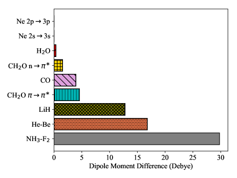
Figure 1: The norms of the dipole moment differences between ground and excited states. The BHHLYP functional is used in all dipole calculations.

III.3 Single-CSF Excited States

Let us begin with an analysis of how the theory performs for excited states dominated by a single CSF, looking at different types of excitations within this category. We will look first at valence excitations, followed by CT states and finally Rydberg excitations. These cases covered, we will then consider states that contain a superposition of multiple CSFs.

III.3.1 Valence Excitations

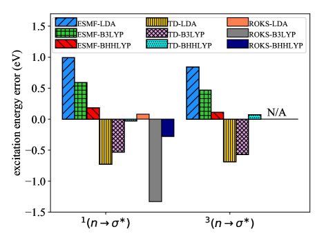
Figure 2: The excitation energy error of singlet (left) and triplet (right) $n\rightarrow\sigma^{\ast}$ excited states in H₂O compared to EOM-CCSD results.

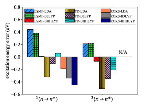
Figure 3: The excitation energy error of singlet (left) and triplet (right) $n\rightarrow\pi^{\ast}$ excited states in CH₂O compared to EOM-CCSD results.

Excitation energy errors relative to EOM-CCSD for H₂O and CH₂O are shown in Figures 2 and 3, respectively. Compared to the CT examples in the next section, TDDFT performs relatively well for these valence excitations, with B3LYP and especially BHHLYP providing excitation energies within about half an eV of the reference and LDA performing only a little worse. These relatively good TDDFT results are not particularly surprising in light of the fact that the charge density deformations are small, and so the lack of orbital relaxation due to the AA is not especially concerning. In fact, we have explicitly analyzed the importance of orbital relaxation by evaluating the Frobenius norm of the DFE-ESMF orbital rotation matrix $\bm{X}$. Averaging over the three values from the three different functionals tested, we find $||\bm{X}||$ to be 0.16 and 0.15 for H₂O and CH₂O, respectively, which is smaller than in the CT examples we will see below.

The basic trend in DFE-ESMF accuracies for different functionals follows that of TDDFT in these excitations, with BHHLYP giving the most accurate predictions, followed by B3LYP and then LDA. As we will see, the accuracy ordering for different functionals in DFE-ESMF plays out is the same way in most of our test systems, with BHHLYP’s high fraction of wave function exchange outperforming the other two functionals in valence, CT, and Rydberg states. Our understanding of this trend is that a larger fraction of wave function exchange is most likely helping to balance self-interaction errors in the ground and excited states. We expect that these errors are larger in the excited states due to their open-shell nature, and so a higher fraction of wave function exchange than is typically used in ground state models appears to be helpful for balancing these errors between the ground and excited states. We should emphasize that in all of our DFE-ESMF results, energy differences were evaluated based on the same functional for both ground and excited states, but using the density and wave function exchange definition for the state in question (see discussion surrounding Eq. (30)). Although this preliminary test of four single-CSF valence excitations is far from exhaustive or systematic, the efficacy of DFE-ESMF/BHHLYP in these cases provides an encouraging proof of principle.

For singlet excited states, we also compare to the predictions of ROKS, which, like DFE-ESMF, provides excited state orbital relaxation. The most striking difference between the ROKS results and those of TDDFT and DFE-ESMF is that they do not follow the same trend with respect to the fraction of wave function exchange. Indeed, the accuracy ordering differs in H₂O and CH₂O, with LDA seeming to offer the best average ROKS performance and with ROKS/B3LYP delivering a surprisingly large error in H₂O. Note that we have not carried out ROKS comparisons in the triplet states because QChem currently only implements ROKS for singlet states.

III.3.2 Charge-Transfer Excitations

Although DFE-ESMF and TDDFT provide similar accuracies in the simple valence excitations discussed above, the story is very different for CT excitations. Before looking in detail at the numerical CT examples, it is worth considering two important potential sources of error TDDFT faces in CT contexts, which we will refer to as the EA/IP imbalance and the orbital relaxation error. To see these clearly, consider a simple CT excitation consisting of a single $i\rightarrow a$ transition, in which case the TDDFT excitation energy is given by Baerends, Gritsenko, and van Meer (2013)

$$\Delta E(i\rightarrow a)=\epsilon_{a}^{KS}-\epsilon_{i}^{KS}+\left<ia|f_{xc}|ia\right>$$ (40)

in which $\epsilon_{i}^{KS}$ and $\epsilon_{a}^{KS}$ are the ground state KS orbital energies of the donor and acceptor orbitals, respectively. This equation has been used extensivelyDreuw, Weisman, and Head-Gordon (2003); Dreuw and Head-gordon (2005); Maitra (2016, 2017) to analyze the TDDFT’s failure in CT excited states and we refer readers to those references for details. In a nutshell, because $\epsilon_{a}^{KS}$ does not correspond to the EA of the acceptor (it undercounts the new repulsions created by the extra electron), the orbital energy difference in this equation tends to severely underestimate CT excitation energies. In principle this should be repaired by the xc term, but the error is often much larger than existing functionals, even RSHs, can correct for.

While the EA/IP imbalance is a significant concern, it is typically offset in practice by the fact that TDDFT works with unrelaxed orbitals. It is well known in electronic structure theory that the omission of orbital relaxation effects tends to raise the energy of the excited state. Ideally, the third term in Equation 40 would eliminate both orbital relaxation issues and the EA/IP imbalance, but even when the third term is zero, these two errors do at least work to cancel each other because they push in opposite directions. However, the EA/IP imbalance in long-range CT is often much too large for orbital relaxation errors to counteract, resulting in TDDFT excitation energies that are much too low as in the NH${}_{3}\rightarrow$F₂ and He$\rightarrow$Be transitions shown below. However, as one moves to increasingly shorter range CT with correspondingly larger overlaps between the donor and acceptor, the EA/IP imbalance becomes less and less of an error and more and more a positive feature of the TDDFT formalism. Indeed, in the valence excitation limit, the difference in how DFT accounts for electron-electron repulsion energy in the occupied and virtual orbitals increases the accuracy of using orbital energy differences as excitation energy estimates, because in this limit the “donor” and “acceptor” are one and the same. One can imagine that for very short-ranged CT, any small remaining errors from the EA/IP imbalance could cancel with orbital relaxation errors precisely enough for the exchange correlation term to clean up the details. Such an effect seems to be at work in LiH, to which we now turn our attention, which despite having a substantial dipole change and thus CT is nonetheless treated well by TDDFT.

LiH

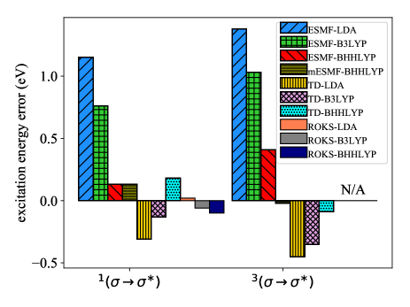
Figure 4: The excitation energy error of singlet (left) and triplet (right) $\sigma\rightarrow\sigma^{\ast}$ excited states in LiH compared to EOM-CCSD results.

Figure 4 shows excitation energy errors for the lowest singlet and triplet excitations in LiH. For both of these states, the balancing process between EA/IP issues and missing orbital relaxations appears to work in TDDFT’s favor, especially in the case of the BHHLYP functional. To check that such a trade off really does appear to be at work here, we again evaluated $||\bm{X}||$ as a measure of orbital relaxation importance and found it to be 0.41, significantly higher than for H₂O or CH₂O. As in the valence states of those molecules, BHHLYP is also very effective in DFE-ESMF’s single-CSF formalism for LiH’s singlet excitation. For the triplet, however, the single-CSF formalism shows relatively poor accuracy regardless of functional, and indeed this state has more than one CSF above our $\epsilon=0.2$ threshold in TDDFT. When we include both of the CSFs whose coefficients breach this threshold via the multi-CSF approach, the DFE-ESMF/BHHLYP result improves from an error above 0.4 eV to an error of just -0.02 eV relative to EOM-CCSD. Note that the multi-CSF approach has no effect on the singlet state, as in that case only the primary CSF was above the threshold.

NH₃ to F₂

We now turn our attention to the first of two long-range CT excitations: the NH₃-F₂ dimer shown in Figure S1. In Figure 5, we see that, after excited-state orbital relaxation via the minimization of Eq. (18), DFE-ESMF is substantially more accurate than TDDFT regardless of the functionals chosen. Even when comparing ESMF-LDA against TDDFT with the $\omega$B97X RSH, the variational approach makes an excitation energy error roughly half as large. Using BHHLYP, which continues to outperform the others for DFE-ESMF, the variational approach achieves an excitation energy error of just 0.26 eV, compared to multi-eV errors for TDDFT when using either $\omega$B97X or BHHLYP.

Although this excited state is predominantly a HOMO$\rightarrow$LUMO excitation, we find that ROKS consistently collapses to a lower excited state (see the Appendix for absolute excitation energies). Hence, we compare our results to MOM $\Delta$SCF instead. We found that $\Delta$SCF DFT yields similarly accurate predictions as DFE-ESMF. This is as expected since $\Delta$SCF DFT are known to perform well in long-range CT excited states, if the states are dominated by one CSF.

It would appear that TDDFT’s error cancellation between its EA/IP imbalance and its lack of orbital relaxations breaks down here, with the magnitude of the former overwhelming that of the latter. We can verify this picture in two ways: first, with the DFE-ESMF approach, and second, by looking at ground state KS-DFT IP-EA estimates at very long range. Start with DFE-ESMF. At the top of Figure 5, we show the excitation energies (i.e. the energy differences between Eq. (30) and the ground state KS energy) before the DFE-ESMF orbital optimization has been carried out, meaning that the excited state DFE-ESMF energy is being evaluated using the ground state KS orbitals. This excitation energy is thus the difference between two many-electron DFT energies (one DFE-ESMF and one KS-DFT) and so does not suffer from the EA/IP imbalance. While the EA/IP issue has thus been removed, orbital relaxation effects have yet to be included, and as expected the excitation energies are now too large. When we then relax the orbitals ($||\bm{X}||=0.21$), we see in the middle of Figure 5 that the predicted excitation energies decrease to more accurate values. Thus, by looking step-wise at how DFE-ESMF changes the energy from TDDFT, we can watch the staged removal of first the EA/IP imbalance and then the fixed-orbital error. This process appears to confirm the idea that TDDFT suffers from both, and that in long-range CT the EA/IP part dominates, leading TDDFT to underestimate the excitation energy.

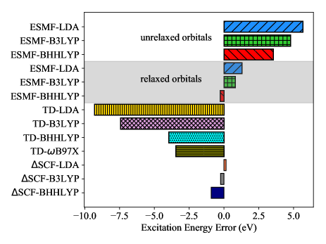
Figure 5: Comparison of excitation energy errors relative to EOM-CCSD for the NH₃ 2pz $\rightarrow$F₂ 2pz CT excitation at an intermolecular separation of 6 $\mathring{A}$. For DFE-ESMF, we show the results both before and after the orbital relaxation is performed.

We can corroborate this view by moving the molecules to a very large distance and comparing DFE-ESMF, TDDFT, and a simple difference of ground state KS energies between the cation, anion, and neutral species that provides a many-electron evaluation of the IP and EA. At very long distance, Figure 6 shows that the performance of DFE-ESMF and TDDFT is quite similar to what we saw at the shorter separation. At the bottom of the figure, we see that if we simply perform four single-molecule ground state KS calculations for the donor cation, acceptor anion, and the two neutral species, the resulting difference between the IP and EA is a very accurate predictor of the charge transfer energy, as we would expect from previous work on CDFT. Thus, if both the IP/EA imbalance born of single-particle orbital energy differences and the orbital relaxation errors are removed via this ground state KS approach or by CDFT, accuracy is restored. The key point is that, unlike these approaches, the DFE-ESMF formalism should allow both of these issues to be addressed even in systems where clear-cut foreknowledge distinguishing between the donor and acceptor is not available, and without having to worry about the spin-symmetry breaking inherent to $\Delta$SCF.

Figure 6: Excitation energy errors relative to EOM-CCSD for the NH₃ 2pz $\rightarrow$F₂ 2pz CT at a 120 $\mathring{A}$ intermolecular separation. $\omega$B97X-IPEA refers to the difference between (a) the sum of ground state KS energies for the donor cation and acceptor anion and (b) the ground state KS energy of the neutral ground states.

He to Be

In our second long-range CT example, we investigate the excitation from the He 1s orbital to the Be 2pz orbital as a function of the distance between the atoms. In Figure 7, we see the familiar failure of local functionals and simple hybrids to predict the correct $1/R$ trend in the excitation energy. While this problem is repaired by the use of a RSH, we see that absolute accuracy is still poor, at least for the specific $\omega$B97X functional we tested here. As in the previous example, DFE-ESMF out-performs the accuracy of the RSH regardless of which functional it is paired with while also correctly capturing the $1/R$ behavior. The advantage of DFE-ESMF becomes especially clear when looking at the non-parallelity error (NPE) plotted in Figure 8, which is defined as the difference between the largest and smallest errors relative to EOM-CCSD across the distance coordinate. DFE-ESMF with LDA, B3LYP, and BHHLYP all produce NPEs below 1eV, as compared to an NPE of almost 2 eV for TDDFT with the $\omega$B97X functional.

While $\Delta$SCF produces a visibly not-smooth curve when when paired with the LDA functional (possibly due to variational collapse issues), its performance with B3LYP and BHHLYP is quite good. In the long-range limit these potential curves overlap that of EOM-CCSD, although accuracy is a bit lower at shorter ranges where the broken spin symmetry is expected to matter more. Consequently, the NPEs of $\Delta$SCF with the hybrid functionals are a bit larger than those of DFE-ESMF, but a major improvement over TDDFT.

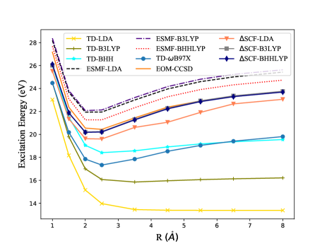
Figure 7: Comparison of He 1s$\rightarrow$Be 2p CT excitation energy as a function of $R$(He-Be) between DFE-ESMF, TDDFT, $\Delta$SCF, and EOM-CCSD.

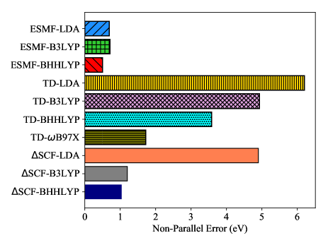
Figure 8: Comparison of non-parallelity errors in the He 1s$\rightarrow$Be 2p CT excitation energy.

III.3.3 Rydberg Excitations

Unlike in CT excitations, it is not obvious that the ability of DFE-ESMF to address the EA/IP imbalance and orbital relaxations will be of great benefit in the context of Rydberg excitations. In these states, the challenge faced by TDDFT arises primarily from the failure of practical xc functionals to produce a potential that decays as $1/r$ at large distances, which is not the same as the failure of error cancellation that causes trouble in the CT case. However, work by Van Voorhis Cheng, Wu, and Voorhis (2008) has shown that although the ground state xc potential has little resemblance to the exact potential, the xc potential associated with an excited state density can behave much more sensibly at long distance. Thus, it is interesting to ask whether DFE-ESMF’s inherently excited state nature and its ability to relax the orbitals in an excited-state-specific manner may in practice lead to improvements for Rydberg states.

As an initial probe of this question, we have studied the 2s$\rightarrow$3s excitation in the Ne atom. The excitation energy error relative to EOM-CCSD is plotted in Figure 9. As expected, TDDFT drastically underestimates the excitation energy by as large as 8.21eV using LDA and 2.94eV using BHHLYP. Notably, although our DFE-ESMF method is able to reduce the error of TDDFT by some amount, it is still very far from being quantitatively accurate. The most accurate functional in DFE-ESMF, the BHHLYP functional, still underestimates the excitation energy by 2.74eV. Although there is no dipole change in this excitation, the charge deformation in Rydberg states is still large since the virtual orbitals are much more diffuse than and share little overlap with the occupied orbitals. Consequently, the averaged $||\bm{X}||$ is as large as 0.25, comparable to that of CT excitations, indicating that orbital relaxation is also important in Rydberg excitations.

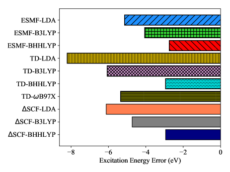
Figure 9: Comparison of excitation energy error of the Ne 2s $\rightarrow$ 3s transition.

As discussed in the previous subsection, the main source of error in DFE-ESMF is the self-interaction error with approximate xc functionals: The functional parametrized for the ground state is incapable of correcting the self-interaction error of the excited electron residing in virtual orbitals. This problem is not too concerning in valence excitations since the occupied and virtual orbitals have similar characters, and hence similar amount of self-interaction. Therefore thanks to error cancellation, balanced description between the ground and the excited states can still be achieved. However, in Rydberg states, the virtual orbitals are much more diffuse than the occupied orbitals. Consequently, the amount of SIEs left in $J[n]$ after adding the UEG exchange energy $E^{UEG}_{x}[n]$ to it, as in LDA, becomes clearly different in the occupied and virtual orbitals. This results in an unbalanced treatment between the ground and the excited state if one uses the same xc functionals for both states, leading to a large error in this Rydberg excitation energy. In future, testing asymptotically corrected functionals in DFE-ESMF would appear to be warranted.

The unbalanced treatment of SIEs should not be exclusive to DFE-ESMF and could affect $\Delta$SCF DFT as well, since it also uses ground state functionals to describe excited states. In fact, in Figure 9 we found that the size and trend of errors of $\Delta$SCF DFT with different xc functionals is quite comparable to DFE-ESMF, corroborating our speculations. In this case, the recovery of spin-symmetry in DFE-ESMF does not appear to have had much effect on the excitation energy.

III.4 Multi-CSF Excited States

We now turn our attention to states in which multiple CSFs are important. While DFE-ESMF can be formulated to treat such states and thus may be expected to offer a significant advantage over single-determinant methods such as $\Delta$SCF, such optimism must be tempered by the increased risk of making double counting errors and the complication of needing a way to choose the values of the CI coefficients. As we see in the following subsections, these issues result in the present formulation of DFE-ESMF being less effective in the multi-CSF case than it was in the single-CSF cases discussed above.

CH₂O

The $\pi\rightarrow\pi^{\ast}$ excited state in CH₂O contains significant contributions from two excited CSFs: HOMO-1$\rightarrow$LUMO and HOMO$\rightarrow$LUMO+2. In contrast to LiH, where TDDFT only predicts multiple important CSFs for the BHHLYP functional, this CH₂O excitation is strongly multi-CSF in TDDFT regardless of the choice of funcitonal. Excitation energy errors relative to EOM-CCSD are plotted in Figure 10, where the $\Delta$SCF results have been obtained by optimizing the orbitals for the open-shell determinant that has the largest weight in TDDFT’s CI vector. Curiously, both TDDFT and DFE-ESMF give the most accurate prediction with LDA in this case, with DFE-ESMF showing especially poor accuracy with BHHLYP. This sharp contrast to the trends we saw in the single-CSF cases is explained, at least in part, by the strong dependence of the CI coefficients on the choice of functional. For LDA and B3LYP, the HOMO$\rightarrow$LUMO+2 CSF has a larger weight that the HOMO-1$\rightarrow$LUMO CSF, whereas the relative importance of these CSFs is reversed when using BHHLYP. Noting that $\Delta$SCF places the energy of the orbital-optimized HOMO-1$\rightarrow$LUMO CSF 1.86eV below the energy of the orbital-optimized HOMO$\rightarrow$LUMO+2 CSF, we can understand much of DFE-ESMF/BHHLYP’s lowering of the excitation energy simply in terms of the change in the CI coefficients coming from TDDFT. It therefore appears that, in future, re-optimizing the CI coefficients within the DFE-ESMF framework may be important.

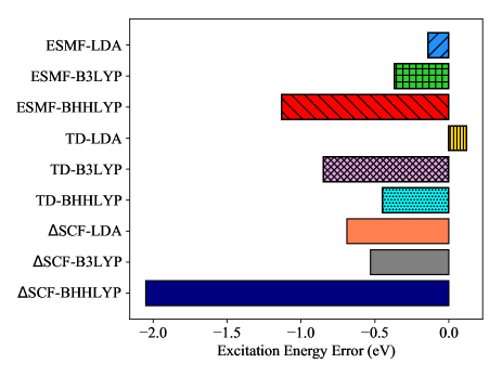
Figure 10: The excitation energy error of singlet $\pi\rightarrow\pi^{\ast}$ excited states in CH₂O compared to EOM-CCSD results.

CO

In the $\pi\rightarrow\pi^{\ast}$ excitation in CO, spatial symmetry ensures that the $p_{x}$ $\pi$ orbital is degenerate with its $p_{y}$ counterpart, and likewise for the two $\pi^{\ast}$ orbitals, so that the excited state is an equal mixture of the $\pi_{x}\rightarrow\pi_{x}^{\ast}$ and $\pi_{y}\rightarrow\pi_{y}^{\ast}$ CSFs. The excitation energy errors for this state are shown in Figure 11, where we have used our multi-CSF formalism to treat this two-CSF state. In this case, the DFE-ESMF trend is back in line with what we saw in most other states, with BHHLYP providing the most accurate result, although TDDFT is notably more accurate than DFE-ESMF. The trend for $\Delta$SCF is quite different, and it faces multiple difficulties here, including the breaking of spin and spatial symmetry as well as variational collapse to the ground state with BHHLYP, which explains the unusually large error in that case.

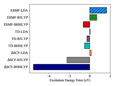
Figure 11: The excitation energy errors relative to EOM-CCSD for the CO $\pi\rightarrow\pi^{\ast}$ singlet excitation. Energy minimization of $\Delta$ SCF with BHHLYP functional ends up collapsing back to ground state.

Ne

Unlike its 2s$\rightarrow$3s excitation, the Ne atom’s 2p$\rightarrow$3p excited state is a equal mixture of two CSFs. In the plot of excitation energy errors (Figure 12) we see that DFE-ESMF and TDDFT have similar accuracies in this case, although the former errors high while the latter errors low. Again, we see the tendency of DFE-ESMF to benefit from a relatively high fraction of wave function exchange. Unlike the other two multi-CSF cases discussed above, $\Delta$SCF proves considerably more accurate for this excitation than either DFE-ESMF or TDDFT.

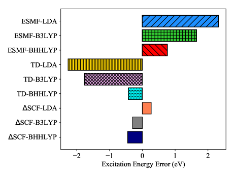
Figure 12: Comparison of excitation energy errors relative to EOM-CCSD for the Ne 2p $\rightarrow$ 3p transition.

IV Conclusions

We have presented a density functional extension to the recently developed excited state mean-field theory in an attempt to capture the effects of weak electron correlation. By augmenting the ESMF wave function’s energy expression with components from density functional theory and inserting the resulting expression into an approximate excited variational principle, the approach provides excited-state-specific orbital optimization in the presence of a correlation treatment. In the same way as KS-DFT closely parallels many aspects of HF theory, this DFE-ESMF approach closely parallels ESMF theory. Being a variational, time-independent approach, the method differs from TDDFT in some important aspects, most notably in its ability to fully relax orbitals and in the fact that it does not depend on the ground state KS orbital eigenvalues and so avoids concerns related to the EA/IP imbalance. In preliminary testing, these advantages result in significantly improved excitation energies for simple charge transfer examples, while accuracy for other excitations is more comparable to TDDFT. Compared to ROKS and $\Delta$SCF, which can also deliver full orbital relaxation, DFE-ESMF is less prone to variational collapse thanks to its use of an excited state variational principle.

Although these advantages and strengths are promising, the current formulation of DFE-ESMF also has a number of shortcomings. For excited states in which multiple CSFs make major contributions, double counting becomes a serious concern and accuracy, although still close to that of TDDFT, is reduced. This challenge is especially concerning in the context of larger systems, where multi-CSF states become increasingly common. Rydberg states are also challenging, although this may have more to do with the choice of density functional than with the DFE-ESMF approach itself: both it and TDDFT make substantial errors in these states. Looking forward, we therefore see a number of directions for possible improvement. As we saw in all cases (except for the $\pi\rightarrow\pi^{*}$ transition in formaldehyde where the sensitivity of TDDFT’s CI coefficients to the fraction of wave function exchange appears to be the culprit) DFE-ESMF was most accurate when using a much higher fraction of wave function exchange (50%) than is typically found in ground state functionals. This is not surprising given the open shell nature of excited states, and suggests that a straightforward route to improved energetics may come from retraining functionals in this direction. Of course, this is just one question in a much broader array of functional design issues, such as whether it would be advantageous to include range-separation or asymptotic corrections, the latter of which may help with the Rydberg problem. Functional design questions aside, our observation that accuracy tends to be lower in multi-CSF states raises the question of whether this is due to relying on TDDFT CI coefficients or comes from some other source. If the former, then variational re-optimization of the CI coefficients alongside the orbitals may be advantageous. Finally, as a practical issue, our pilot implementation achieves the desired cost scaling (equivalent to ground state KS-DFT) but could be sped up considerably if implemented in a production level quantum chemistry package.

Appendix A Molecular Geometries

In H₂O the H-O-H bond angle is chosen to be 104.5^∘ and the O-H bond length is 0.96$\mathring{A}$. In CH₂O the H-C-H bond angle is 116^∘, and the C-H and C-O bond length are 1.11$\mathring{A}$ and 1.21$\mathring{A}$ respectively. In LiH the bond length is 1.6$\mathring{A}$, and the He-Be separation is 3.5$\mathring{A}$. The geometry of the NH₃-F₂ dimer is shown in Figure 13.

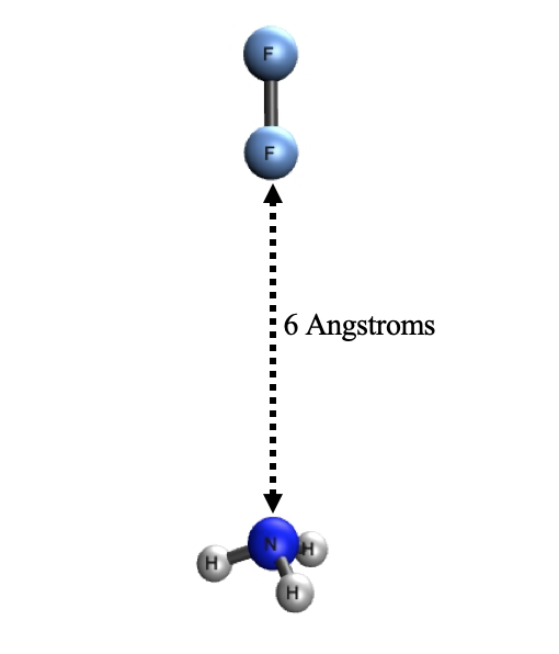
Figure 13: Geometry of the NH₃-F₂ dimer. The N-H bond length and H-N-H bond angle is 1.02$\mathring{A}$ and 106.2^∘. The F₂ bond length is 1.43$\mathring{A}$.

Appendix B Absolute Excitation Energies

The absolute excitation energies studied in this work is shown in Table 1, 2, 3, and 4.

Table 1: Excitation energies of DF-ESMF and EOM-CCSD for the system studied in eV. Note that the BHHLYP excitation energy of LiH ³($\sigma\rightarrow\sigma^{\ast}$) state is from the single-CSF formalism, and the corresponding excitation energy is 3.07eV if the multi-CSF formalism is used.

	LDA		B3LYP		BHHLYP		EOM-CCSD
H2O 1(n$\rightarrow\pi^{\ast}$)	9.	07	8.	66	8.	26	8.	07
H2O 3(n$\rightarrow\pi^{\ast}$)	8.	23	7.	86	7.	50	7.	39
LiH 1($\sigma\rightarrow\sigma^{\ast}$)	4.	62	4.	23	3.	60	3.	47
LiH 3($\sigma\rightarrow\sigma^{\ast}$)	4.	47	4.	12	3.	50	3.	09
CH2O 1(n$\rightarrow\pi^{\ast}$)	4.	57	4.	51	4.	13	4.	13
CH2O 3(n$\rightarrow\pi^{\ast}$)	3.	85	3.	86	3.	57	3.	64
CH2O 1($\pi\rightarrow\pi^{\ast}$)	9.	94	9.	71	8.	93	10.	08
CO 1($\pi\rightarrow\pi^{\ast}$)	7.	13	6.	17	4.	86	5.	49
NH3-F2	10.	59	10.	12	9.	03	9.	29
Ne 2s$\rightarrow$3s	42.	16	43.	24	44.	56	47.	30
Ne 2p$\rightarrow$3p	22.	36	21.	69	20.	79	20.	04

Table 2: Excitation energies of TDDFT for the system studied in eV.

	LDA		B3LYP		BHHLYP		$\omega$B97X
H2O 1(n$\rightarrow\pi^{\ast}$)	7.	34	7.	54	8.	14	N/A
H2O 3(n$\rightarrow\pi^{\ast}$)	6.	70	6.	82	7.	36	N/A
LiH 1($\sigma\rightarrow\sigma^{\ast}$)	3.	16	3.	34	3.	65	N/A
LiH 3($\sigma\rightarrow\sigma^{\ast}$)	2.	64	2.	74	3.	00	N/A
CH2O 1(n$\rightarrow\pi^{\ast}$)	3.	81	4.	02	4.	18	N/A
CH2O 3(n$\rightarrow\pi^{\ast}$)	3.	13	3.	29	3.	43	N/A
CH2O 1($\pi\rightarrow\pi^{\ast}$)	9.	23	9.	63	10.	12	N/A
CO 1($\pi\rightarrow\pi^{\ast}$)	5.	52	5.	21	4.	99	N/A
NH3-F2	0.	00	1.	88	5.	32	5.	84
Ne 2s$\rightarrow$3s	39.	09	41.	23	44.	36	41.	95
Ne 2p$\rightarrow$3p	17.	78	18.	27	19.	60	N/A

Table 3: Excitation energies of ROKS for the system studied in eV.

	LDA		B3LYP		BHHLYP		$\omega$B97X
H2O 1(n$\rightarrow\pi^{\ast}$)	8.	15	6.	75	7.	79	N/A
LiH 1($\sigma\rightarrow\sigma^{\ast}$)	3.	48	3.	41	3.	37	N/A
CH2O 1(n$\rightarrow\pi^{\ast}$)	3.	94	3.	79	3.	68	N/A
NH3-F2	-5.	50	-5.	53	-5.	26	-5.	24

Table 4: Excitation energies of $\Delta$SCF-DFT for the system studied in eV.

	LDA		B3LYP		BHHLYP		$\omega$B97X
CH2O 1($\pi\rightarrow\pi^{\ast}$)	9.	38	9.	55	8.	03	N/A
CO 1($\pi\rightarrow\pi^{\ast}$)	5.	64	3.	26	0.	00	N/A
NH3-F2	9.	45	9.	06	8.	38	9.	10
Ne 2s$\rightarrow$3s	41.	18	42.	57	44.	36	43.	15
Ne 2p$\rightarrow$3p	20.	31	19.	73	19.	58	N/A