On Value Functions and the Agent-Environment Boundary

Abstract

When function approximation is deployed in reinforcement learning (RL), the same problem may be formulated in different ways, often by treating a pre-processing step as a part of the environment or as part of the agent. As a consequence, fundamental concepts in RL, such as (optimal) value functions, are not uniquely defined as they depend on where we draw this agent-environment boundary. This causes further problems in theoretical analyses that provide optimality guarantees, as the same analysis may yield different bounds in equivalent formulations of the same problem. We address this issue via a simple and novel boundary-invariant analysis of Fitted Q-Iteration, a representative RL algorithm, where the assumptions and the guarantees are invariant to the choice of boundary. We also discuss closely related issues on state resetting, deterministic vs stochastic systems, imitation learning, and the verifiability of theoretical assumptions from data.

1 Introduction

A large part of RL theory—including that on function approximation—is built on mathematical concepts established in the Markov Decision Process (MDP) literature (Puterman, 1994), such as the optimal state- and $Q$-value functions ($V^{\star}$ and $Q^{\star}$) and their policy-specific counterparts ($V^{\pi}$ and $Q^{\pi}$). These functions operate on the state (and action) of the MDP, and classical results tell us that they are always uniquely and well defined.

Are they really well defined?

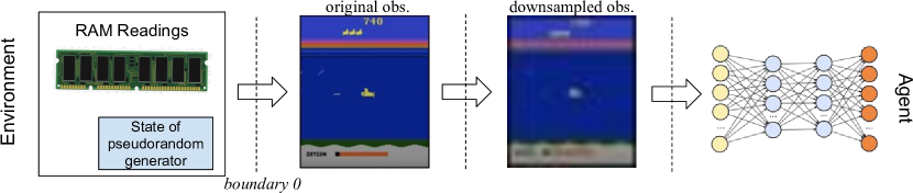
Figure 1: Illustration of the agent-environment boundaries. Strickly speaking, the environments defined by the intermediate boundaries are partially observable, but we can view them as MDPs over histories (of actions and observations defined by the boundary). Therefore, partial observability has little to do with our concerns, and we stick to MDP terminologies in the main text and do not invoke POMDP concepts for simplicity and clarity.

Consider the following scenario, depicted in Figure 1. In a standard ALE benchmark (Bellemare et al., 2013), raw-pixel screens are produced as states (or strictly speaking, observations), and the agent feeds the state into a neural net to predict $Q^{\star}$. Since the original game screen has a high resolution, it is common in practice to downsample the screen as a pre-processing step (Mnih et al., 2015).

There are two equivalent views of this scenario: We can view the pre-processing step as part of the environment, or as part of the agent. Depending on where we draw this agent-environment boundary, $Q^{\star}$ will be different in general. It should also be obvious that there may exist many choices of the boundary (e.g., “boundary 0” in Figure 1), some of which we may be even not aware of. When we design an algorithm to learn $Q^{\star}$, which $Q^{\star}$ are we talking about?

The good news is that many existing algorithms are boundary invariant, that is, once the function approximation scheme is fixed, the boundary is only a subjective choice and does not affect the behavior of the algorithm. The bad news is that many existing analyses are boundary dependent, as they make assumptions that may either hold or fail in the same problem depending on the choice of the boundary: for example, in the analyses of approximate value iteration algorithms, it is common to assume that $Q^{\star}$ can be represented by the function approximator (“realizability”), and that the function space is closed under Bellman update (low “inherent Bellman error”, Szepesvári and Munos, 2005; Antos et al., 2008), both of which are boundary-dependent assumptions. Such a gap between the mathematical theory and the reality also leads to further consequences, such as the theoretical assumptions being fundamentally unverifiable from naturally generated data.

In this paper we systematically study the boundary dependence of RL theory. We ground our discussions in a simple and novel boundary-invariant analysis of Fitted Q-Iteration (Ernst et al., 2005), in which the correctness of the assumptions and the guarantees do not change with the subjective choice of the boundary (Sections 4 and 5). Within this analysis, we give up on the classical notions of value functions or even the (state-wise) Bellman equation, and replace them with weaker conditions that are boundary invariant. We also discuss closely related issues regarding state resetting, deterministic versus stochastic systems, imitation learning, and the verifiability of theoretical assumptions from data (Section 6). The implications drawn from our results suggest novel ways of thinking about states, value functions, and optimality in RL.

2 Preliminaries

Markov Decision Processes   An infinite-horizon discounted MDP $M$ is specified by $(\mathcal{S},\mathcal{A},P,R,\gamma,d_{0})$, where $\mathcal{S}$ is the finite state space, $\mathcal{A}$ is the finite action space, $P:\mathcal{S}\times\mathcal{A}\to\Delta(\mathcal{S})$ is the transition function, $R:\mathcal{S}\times\mathcal{A}\to\Delta([0,R_{\max}])$ is the reward function, $\gamma\in[0,1)$ is the discount factor, and $d_{0}\in\Delta(\mathcal{S})$ is the initial state distribution.

A (stationary and deterministic) policy $\pi:\mathcal{S}\to\mathcal{A}$ specifies a decision-making strategy, and induces a distribution over random trajectories: $s_{1}\sim d_{0}$, $a_{1}\sim\pi$, $r_{1}\sim R(s_{1},a_{1})$, $s_{2}\sim P(s_{1},a_{1})$, $a_{2}\sim\pi$, …, where $a_{t}\sim\pi$ is short for $a_{t}=\pi(s_{t})$. In later analyses, we will also consider stochastic policies $\pi:\mathcal{S}\to\Delta(\mathcal{A})$ and non-stationary policies formed by concatenating a sequence of stationary ones.

The performance of a policy $\pi$ is measured by its expected discounted return (or value):

$$\textstyle v^{\pi}:=\mathbb{E}[\sum_{t=1}^{\infty}\gamma^{t-1}r_{t}~{}\big{|}~{}s_{1}\sim d_{0},\,a_{1:\infty}\sim\pi].$$

The value of a policy lies in the range of $[0,V_{\max}]$ with $V_{\max}=R_{\max}/(1-\gamma)$. It will be useful to define the $Q$-value function of $\pi$: $\textstyle Q^{\pi}(s,a):=\mathbb{E}[\sum_{t=1}^{\infty}\gamma^{t-1}r_{t}~{}\big{|}~{}s_{1}=s,a_{1}=a,\,a_{2:\infty}\sim\pi],$ and $d_{t}^{\pi}$, the distribution over state-action pairs induced at time step $t$: $d_{t}^{\pi}(s,a):=\Pr[s_{t}=s,a_{t}=a~{}\big{|}~{}s_{1}\sim d_{0},\,a_{1:\infty}\sim\pi].$ Note that $d_{1}^{\pi}=d_{0}\times\pi$, which means $s\sim d_{0},a\sim\pi$.

The goal of the agent is to find a policy $\pi$ that maximizes $v^{\pi}$. In the infinite-horizon discounted setting, there always exists an optimal policy $\pi^{\star}$ that maximizes the expected discounted return for all states simultaneously (and hence also for $d_{0}$). Let $Q^{\star}$ be a shorthand for $Q^{\pi^{\star}}$. It is known that $\pi^{\star}$ is the greedy policy w.r.t. $Q^{\star}$: For any $Q$-function $f$, let $\pi_{f}$ denote its greedy policy $(s\mapsto\operatorname*{arg\,max}_{a\in\mathcal{A}}f(s,a))$, and we have $\pi^{\star}=\pi_{Q^{\star}}$. Furthermore, $Q^{\star}$ satisfies the Bellman equation: $Q^{\star}=\mathcal{T}Q^{\star}$, where $\mathcal{T}:\mathbb{R}^{\mathcal{S}\times\mathcal{A}}\to\mathbb{R}^{\mathcal{S}\times\mathcal{A}}$ is the Bellman optimality operator:

$$(\mathcal{T}f)(s,a)=\mathbb{E}_{r\sim R(s,a),s^{\prime}\sim P(s,a)}[r+\gamma\max_{a^{\prime}\in\mathcal{A}}f(s^{\prime},a^{\prime})].$$

Value-function Approximation  In complex problems with high-dimensional observations, function approximation is often deployed to generalize over the large state space. In this paper we take a learning-theoretic view of value-function approximation: We are given a function space $\mathcal{F}\subset(\mathcal{S}\times\mathcal{A}\to[0,V_{\max}])$, and for simplicity we assume $\mathcal{F}$ is finite. The goal—stated in the classical, boundary-dependent fashion—is to identify a function $f\in\mathcal{F}$ such that $f\approx Q^{\star}$, so that $\pi_{f}$ is a near-optimal policy. This naturally motivates a common assumption, known as realizability, that $Q^{\star}\in\mathcal{F}$, which will be useful for later discussions.

For most of the paper we will be concerned with batch-mode value-function approximation, that is, the learner is passively given a dataset consisting of tuples $(s,a,r,s^{\prime})$ and cannot directly interact with the environment. The implications in the exploration setting will be briefly discussed at the end of the paper.

Fitted Q-Iteration (FQI)  FQI (Ernst et al., 2005; Szepesvári, 2010) is a batch RL algorithm that solves a series of least-squared regression problems with $\mathcal{F}$ to approximate each step of value iteration. It is also considered as the prototype for the popular DQN (Mnih et al., 2015), and often used as a representative of off-policy value-based RL algorithms in empirical studies (Fu et al., 2019). We defer a detailed description of the algorithm to Section 5.1.

3 Case Study: Boundary Dependence in Batch Contextual Bandit (CB) with Predictable Rewards

To give a concrete instance of how standard theory is boundary dependent, we consider the simplified setting of contextual bandits, which may be viewed as episodic MDPs with $\gamma=0$; here each trajectory only lasts for 1 step and the initial state distribution $d_{0}$ corresponds to the context distribution of the CB (Langford and Zhang, 2008). In CB, FQI degrades to fitting the reward function via squared loss regression. In the rest of this section we will introduce the setting and the algorithm formally, and provide a minimal example to illustrate how difference choices of the boundaries can result in different bounds in the same problem.

3.1 Setting

Let $D=\{(s_{i},a_{i},r_{i})\}$ be a dataset, where $s_{i}\sim d_{0}$, $a_{i}\sim\pi_{b}$ and $r_{i}\sim R(s_{i},a_{i})$. Here $\pi_{b}$ is a behavior policy with which we collect the data. Let $\mu$ denote the joint distribution over $(s,a)$, or $\mu:=d_{0}\times\pi_{b}$. For any $f\in\mathcal{F}$, define the empirical squared loss

$$\textstyle\mathcal{L}_{D}(f):=\frac{1}{|D|}\sum_{i}(f(s_{i},a_{i})-r_{i})^{2},$$ (1)

and the population version $\mathcal{L}_{\mu}(f):=\mathbb{E}_{D}[\mathcal{L}_{D}(f)].$ The algorithm fits a reward function by minimizing $\mathcal{L}_{D}(\cdot)$, that is, ${\hat{f}}:=\operatorname*{arg\,min}_{f\in\mathcal{F}}\mathcal{L}_{D}(f),$ and outputs $\pi_{\hat{f}}$. We are interested in providing a guarantee to the performance of this policy, that is, the expected reward obtained by executing $\pi_{\hat{f}}$, $v^{\pi_{\hat{f}}}=\mathbb{E}[r~{}\big{|}~{}\pi_{\hat{f}}].$ We will base our analyses on the following inequality:

$$\mathcal{L}_{\mu}({\hat{f}})-\min_{f\in\mathcal{F}}\mathcal{L}_{\mu}(f)\leq\epsilon.$$ (2)

In words, we assume that ${\hat{f}}$ approximately minimizes the population loss. Such a bound can be obtained via a uniform convergence argument, where $\epsilon$ will depend on the sample size $|D|$ and the statistical complexity of $\mathcal{F}$ (e.g., pseudo-dimension (Haussler, 1992)). We do not include this part as it is standard and orthogonal to the discussions in this paper, and rather focus on how to provide a guarantee on $v^{\pi_{\hat{f}}}$ as a function $\epsilon$.

3.2 Classical Assumptions and Guarantees

We now review the classical assumptions in this problem for later references and comparisons. The first assumption is that data is exploratory, often guaranteed by taking randomized actions in the data collection policy (or behavior policy $\pi_{b}$) and not starving any of the actions:

Assumption 1 ($\pi_{b}$ is exploratory).

There exists a universal constant $C<+\infty$ s.t., $\forall s\in\mathcal{S},a\in\mathcal{A}$,    $\pi_{b}(a|s)\geq 1/C.$

Next is realizability as already discussed in Section 2.

Assumption 2 (Realizability).

$Q^{\star}\in\mathcal{F}$. In contextual bandits, $Q^{\star}(s,a)=\mathbb{E}[r\,|\,s,a]$, $\forall(s,a)$, which is the reward function.

With these two assumptions, the standard guarantee is the following:

Theorem 1.

Under Assumptions 1 and 2,
$v^{\pi_{\hat{f}}}\geq v^{\star}-2\sqrt{C\epsilon}.$

The proof is omitted as the theorem will be subsumed by more general results. (It is a corollary of either Theorem 2 or 4). Due to the straightforwardness of the analyses and that most CB literature focus on the online setting, we are unable to find an appropriate citation, but we believe readers familiar with the literature will agree that this is a natural setup and analysis for the batch setting.

3.3 Illustration of Boundary Dependence

$Q(s_{A})=Q(s_{B})=0.5$

(a)

$Q^{\prime}(s)=0.5$

(b)

Figure 2: Illustration of two different formulations of the same problem when function approximation is deployed. (a) A contextual bandit with two contexts, $s_{A}$ and $s_{B}$, which appear with equal probabilities, i.e., $d_{0}(s_{A})=d_{0}(s_{B})=0.5$. The only action yields $+1$ reward and $+0$ reward in $s_{A}$ and $s_{B}$, respectively. The function approximator contains only 1 function $Q(s_{A})=Q(s_{B})=0.5$ (action omitted since there is only 1 action). (b) A contextual bandit with one context $s$. The only action available yields a Bernoulli distributed stochastic reward. The function approximator contains only 1 function $Q^{\prime}(s)=0.5$.

We are now ready to illustrate the boundary dependence of Theorem 1 using a minimal example.

Weaker Sense  We start with a weaker sense of boundary dependence, that the assumptions which Theorem 1 rely on may hold under one boundary and fail under another. Consider the two contextual bandit problems in Figure 2, each equipped with a function class for modeling the reward function. It should be obvious that, from the viewpoint of the learning algorithm described in Section 3.1, the two problems are fundamentally indistinguishable, as (2(a)) becomes (2(b)) when the learner fails to distinguish between $s_{A}$ and $s_{B}$. However, Assumption 2 holds in (2(b)) but fail in (2(a)), as the reward function for (2(a)) is $Q^{\star}(s_{A})=1,Q^{\star}(s_{B})=0$, which is not in the class.

Stronger Sense  Familiar readers may argue that the weaker sense of boundary dependence is not necessarily a problem: although Theorem 1 becomes vacuous when we change the boundary, we can still provide meaningful guarantees by considering the approximation errors in the violation of Assumption 2, like in the following result.

Theorem 2 (Robust version of Theorem 1).

Define $\epsilon_{\textrm{approx}}:=\inf_{f\in\mathcal{F}}\|f-Q^{\star}\|_{\mu}^{2}.$ Under Assumption 1 alone, we have   $v^{\pi_{\hat{f}}}\geq v^{\star}-2\sqrt{C(\epsilon+\epsilon_{\textrm{approx}})}.$

When $\epsilon_{\textrm{approx}}=0$ we recover Theorem 1. As $\epsilon_{\textrm{approx}}$ increases, the guarantee degrades gradually. Unfortunately, such a robustness result does not save the classical analysis from the boundary dependence issue. In fact, the bounds are simply different when we apply Theorem 2 in (2(a)) and (2(b)): when $\epsilon=0$, the value guaranteed for (2(b)) is $0.5$, while that for (2(a)) is $0.5-2\sqrt{0.25}=-0.5$ (here $C=1$), which is much looser!

Of course, no loss should be incurred anyway as there is only 1 action in Figure 2, and this example is only intended to illustrate the inconsistency of the classical analyses when they are applied to different formulations of the same problem. While problem-specific and ad hoc fixes may be plausible, what we present in this paper is a general strategy that provides guarantees competitive to the classical analyses under any boundary, together with interesting implications that require us to rethink the meaning of states, value functions, and optimality in RL.

4 Boundary-Invariant Analysis for Batch CB

4.1 A Sufficient Condition for Boundary Invariance

Before we start the analysis, we first show that the algorithm itself is boundary invariant, leading to a sufficient condition for judging the boundary invariance of analyses. The concept central to the algorithm is the squared loss $\mathcal{L}_{D}(f)$. Although $\mathcal{L}_{D}(f)$ is defined using $(s,a)$, the definition refers to $(s,a)$ exclusively through the evaluation of $f\in\mathcal{F}$ on $(s,a)$, taking expectation over a naturally generated dataset $D$. The data points are generated by an objective procedure (collecting data with policy $\pi_{b}$), and on every data point $(s,a,r)$, $f(s,a)$ is the same scalar regardless of the boundary, hence the algorithmic procedure is boundary-invariant.

Inspired by this, we provide the following sufficient condition for boundary-invariant analyses:

Claim 3.

An analysis is boundary invariant if the assumptions and the optimal value are defined in a way that accesses states and actions exclusively through evaluations of functions in $\mathcal{F}$, with plain expectations (either empirical or population) over natural data distributions.

A number of pitfalls need to be avoided in the specification of such a condition:

1. Restricting the functions to $\mathcal{F}$ is important, as one can define conditional expectations (on a single state) through plain expectations via the use of state indicator functions (or the dirac delta functions for continuous state spaces).

2. Similarly, we need to restrict the set of distributions to those natural ones (formalized later in Definition 2) to prevent expectations on point masses. (See Appendix D for further discussions.)

3. Besides the assumptions, the very notion of optimality also needs to be taken care of, as $v^{\star}:=\mathbb{E}_{s\sim d_{0}}[V^{\star}(s)]$ (the usual notion of optimal value) is also a boundary-dependent quantity. (See Section 6.1 for further discussions.)

That said, this condition is not perfectly rigorous, as we find it difficult to make it mathematically strict without being verbose and/or restrictive. Regardless, we believe it conveys the right intuitions and can serve as a useful guideline for judging the boundary invariance of a theory. Furthermore, the condition provides us with significant mathematical convenience: as long as the condition is satisfied, we can analyze an algorithm under any boundary, allowing us to use the standard MDP formulations and all the objects defined therein (states, actions, their distributions, etc.).

4.2 Assumptions and Analysis

Additional Notations  For any $f:\mathbb{R}^{\mathcal{S}\times\mathcal{A}}$ and any distribution $\nu\in\Delta(\mathcal{S}\times\mathcal{A})$, define $\|f\|_{2,\nu}^{2}:=\mathbb{E}_{(s,a)\sim\nu}[f(s,a)^{2}]$. Since we will only be concerned with weighted $\ell_{2}$ norm, we will abbreviate $\|f\|_{2,\nu}^{2}$ as $\|f\|_{\nu}^{2}$ throughout the paper. To improve readability we will often omit “$r\sim R(s,a)$” when an expectation involves $r$ (and “$s^{\prime}\sim P(s,a)$” for Section 5), and use $\mathbb{E}_{\nu}[f]$ as a shorthand for $\mathbb{E}_{(s,a)\sim\nu}[f(s,a)]$.

Definition 1 (Admissible distributions (bandit)).

Given a contextual bandit problem and a space of candidate reward functions $\mathcal{F}$, we call $\{d_{0}\times\pi_{f}:f\in\mathcal{F}\}$ the space of admissible distributions.

Assumption 3.

There exists a universal constant $C<+\infty$ such that, for any $f,f^{\prime}\in\mathcal{F}$ and any admissible $\nu$,   $\|f-f^{\prime}\|_{\mu}^{2}\leq C\cdot\|f-f^{\prime}\|_{\nu}^{2}.$

Assumption 3 is a direct consequence of Assumption 1, and any $C$ that satisfies the latter also works for the former. The proof is elementary and omitted.

Assumption 4.

There exists $f^{\star}\in\mathcal{F}$, such that for all admissible $\nu$,

$$\mathbb{E}_{\nu}[f^{\star}]=\mathbb{E}_{(s,a)\sim\nu}[r],$$ (3)

and for any $f^{\prime}\in\mathcal{F}$,

$$\mathcal{L}_{\mu}(f^{\prime})-\mathcal{L}_{\mu}(f^{\star})=\|f^{\prime}-f^{\star}\|_{\mu}^{2}.$$ (4)

We say that such an $f^{\star}$ is a valid reward function of the CB w.r.t. $\mathcal{F}$.

Assumption 4 is implied by Assumption 2, as $f^{\star}=Q^{\star}$ satisfies both Eq.(3) and Eq.(4): Eq.(3) can be obtained from $Q^{\star}(s,a)=\mathbb{E}[r|s,a]$ by taking the expectation of both sides w.r.t. $\nu$. Eq.(4) is the standard bias-variance decomposition for squared loss regression when $f^{\star}$ is the Bayes-optimal regressor. Eq.(3) guarantees that $f^{\star}$ still bears the semantics of reward, although no longer in a point-wise manner. Eq.(4) guarantees that $f^{\star}$ can be reliably identified through squared loss minimization, which is specialized to and required by the squared loss minimization approaches. In fact, we provide a counter-example in Appendix B showing that dropping Eq.(4) can result in the failure of the algorithm.

Now we are ready to state the main theorem of this section, whose proof can be found in Appendix C. (Also note that Theorem 1 is a direct corollary of Theorem 4.)

Theorem 4.

Under Assumptions 3 and 4, for any valid $f^{\star}$, we have $v^{\pi_{\hat{f}}}\geq v^{\pi_{f^{\star}}}-2\sqrt{C\epsilon}.$

Comparison to Theorem 2  We compare our boundary-invariant analyses with standard boundary-dependent analyses both in the example of Figure 2 and more generally. Observe that in (2(a)), $Q(s_{A})=Q(s_{B})=0.5$ is considered valid by Assumption 4, so we can directly compete with $v^{\pi_{Q}}=0.5$. The bound is tight when $\epsilon=0$, which is in sharp contrast to the loose bound given by Theorem 2 (see Section 3.3).

More generally, if Assumption 2 holds under any boundary, Assumption 4 holds regardless of how the problem is formulated. Consequently, when $\epsilon=0$ the boundary-invariant bound guarantees an optimal value which cannot be exceeded by any policy in $\{\pi_{f}:f\in\mathcal{F}\}$, while the boundary-dependent bounds are generally loose. It is actually possible to push this further and prove the superiority of boundary-invariant bounds in more general conditions:

Proposition 5.

When Assumptions 3 and 4 hold, Theorem 4 is always as tight as Theorem 2 as long as $\epsilon\leq\epsilon_{\textrm{approx}}/2$.

The proof is deferred to Appendix C. The proposition states that the boundary-invariant guarantee in Theorem 4 is always as tight as the robust result given in Theorem 2, as long as the best function in class measures a boundary-dependent approximation error $\epsilon_{\textrm{approx}}$ that is greater than $\epsilon$, the error due to finite sample effect and/or inexact optimization (Eq.(2)).

Note that the above result only applies when Assumption 4 holds. We do expect that the superiority of boundary-invariant analyses should hold in more general situations—at least in some approximate sense—even when Assumption 4 fails (in which case we will need a robust version of Theorem 4), but the analyses become much more involved and it is unclear if a clean analysis and apple-to-apple comparison can be done, so we leave a deeper investigation to future work.

5 Case Study: Fitted Q-Iteration

With the preparation in Section 4, we now analyze the FQI algorithm, and prove the counterparts of Theorems 1 and 4 for FQI.

The major technical difficulty in this section is that the boundary-invariant counterpart of $Q^{\star}$ is not automatically defined in the boundary-invariant analysis, and we have to establish it from the assumptions without using familiar concepts in MDP literature (e.g., we cannot use the fact that $\mathcal{T}$ is a $\gamma$-contraction under $\ell_{\infty}$ in the boundary-invariant analysis).

5.1 Setting and Algorithm

To highlight the differences between boundary-dependent and boundary-invariant analyses, we adopt a simplified setting assuming i.i.d. data. Interested readers can consult prior works for more general analyses on $\beta$-mixing data (e.g., Antos et al., 2008).

Let $D=\{(s_{i},a_{i},r_{i},s_{i}^{\prime})\}$ be a dataset, where $(s_{i},a_{i})\sim\mu$, $r_{i}\sim R(s_{i},a_{i})$, and $s_{i}^{\prime}\sim P(s_{i},a_{i})$. For any $f,f^{\prime}\in\mathcal{F}$, define the empirical squared loss

$$\textstyle\mathcal{L}_{D}(f;f^{\prime}):=\frac{1}{|D|}\sum_{i}(f(s_{i},a_{i})-r_{i}-\gamma\max_{a^{\prime}\in\mathcal{A}}f^{\prime}(s_{i}^{\prime},a^{\prime}))^{2},$$

and the population version $\mathcal{L}_{\mu}(f;f^{\prime}):=\mathbb{E}_{D}[\mathcal{L}_{D}(f;f^{\prime})]$. The algorithm initializes $f_{1}$ arbitrarily, and

$$\textstyle f_{i}:=\operatorname*{arg\,min}_{f\in\mathcal{F}}\mathcal{L}_{D}(f;f_{i-1}),~{}~{}~{}\text{for~{} $i\geq 2$.}$$

The algorithm repeats this for some $k$ iterations and outputs $\pi_{f_{k}}$. We are interested in providing a guarantee to the performance of this policy.

5.2 Classical Assumptions

Similar to the CB case, there will be two assumptions, one that requires the data to be exploratory, and one that requires $\mathcal{F}$ to satisify certain representation conditions.

Definition 2 (Admissible distributions (MDP)).

A state-action distribution is admissible if it takes the form of $d_{t}^{\pi}$ for any $t$, and any non-stationary policy $\pi$ formed by choosing a policy for each time step from $\{\pi_{f}:f\in\mathcal{F}\}\bigcup\{\pi_{f,f^{\prime}}:f,f^{\prime}\in\mathcal{F}\}$, where $\pi_{f,f^{\prime}}(s):=\operatorname*{arg\,max}_{a\in\mathcal{A}}\max(f(s,a),f^{\prime}(s,a))$.

Assumption 5 ($\mu$ is exploratory).

There exists a universal constant $C<+\infty$ such that for any admissible $\nu$, $\max_{s,a}\frac{\nu(s,a)}{\mu(s,a)}\leq C$.

This guarantees that $\mu$ well covers all admissible distributions. The upper bound $C$ is known as the concentrability coefficient (Munos, 2003), and here we use the simplified version from a recent analysis by Chen and Jiang (2019). See Farahmand et al. (2010) for a more fine-grained characterization of this quantity.

Assumption 6 (No inherent Bellman error).

$\forall f\in\mathcal{F}$, $\mathcal{T}f\in\mathcal{F}$.

This assumption states that $\mathcal{F}$ is closed under the Bellman update operator $\mathcal{T}$. It automatically implies $Q^{\star}\in\mathcal{F}$ (for finite $\mathcal{F}$) hence is stronger than realizability, but replacing this assumption with realizability can cause FQI to diverge (Van Roy, 1994; Gordon, 1995; Tsitsiklis and Van Roy, 1997) or suffer from exponential sample complexity (Dann et al., 2018). We refer the readers to Chen and Jiang (2019) for further discussions on the necessity of this assumption.

Boundary-dependent Guarantee  Just as Theorem 1 is a direct corollary of and immediately subsumed by Theorem 4, the boundary-dependent guarantee for FQI under Assumptions 5 and 6 will be subsumed later by the boundary-invariant guarantee in Theorem 8 (which the readers can verify by referring to Theorem 2 of Chen and Jiang (2019) and its proof), so we do not present the result separately here.

5.3 Boundary-Invariant Assumptions

We give the boundary-invariant counterparts of Assumptions 5 and 6.

Assumption 7.

There exists a universal constant $C<+\infty$ such that, for any $f,f^{\prime}\in\mathcal{F}$ and any admissible state-action distribution $\nu$,     $\|f-f^{\prime}\|_{\nu}^{2}\leq C\|f-f^{\prime}\|_{\mu}^{2}.$

Assumption 8.

$\forall f\in\mathcal{F}$, there exists $g\in\mathcal{F}$ such that for all admissible $\nu$,

$$\mathbb{E}_{\nu}[g]=\mathbb{E}_{(s,a)\sim\nu}[r+\gamma\max_{a^{\prime}\in\mathcal{A}}f(s^{\prime},a^{\prime})],$$ (5)

and for any $f^{\prime}\in\mathcal{F}$,

$$\mathcal{L}_{\mu}(f^{\prime};f)-\mathcal{L}_{\mu}(g;f)=\|f^{\prime}-g\|_{\mu}^{2}.$$ (6)

Define $\mathcal{B}$ as the operator that maps $f$ to an arbitrary (but systematically chosen) $g$ that satisfies the above conditions.

Assumption 8 states that for every $f\in\mathcal{F}$, we can define a contextual bandit problem with random reward $r+\gamma\max_{a^{\prime}\in\mathcal{A}}f(s^{\prime},a^{\prime})$, and there exists $g\in\mathcal{F}$ that is a valid reward function for this problem (Assumption 4). In the classical definitions, the true reward function for this problem is $\mathcal{T}f$, so our $\mathcal{B}$ operator can be viewed as the boundary-invariant version of $\mathcal{T}$.

5.4 Boundary-Invariant Analysis

In Section 3 for contextual bandits, $f^{\star}$ is defined directly in the assumptions, and we use it to define the optimal value in Theorem 4. In Assumptions 7 and 8, however, no counterpart of $Q^{\star}$ is defined. How do we even express the optimal value that we compete with?

We resolve this difficulty by relying on the $\mathcal{B}$ operator defined in Assumption 8. Recall that in classical analyses, $Q^{\star}$ can be defined as the fixed point of $\mathcal{T}$, so we define $f^{\star}$ similarly through $\mathcal{B}$.

Theorem 6.

Under Assumption 8, there exists $f^{\star}\in\mathcal{F}$ s.t. $\|\mathcal{B}f^{\star}-f^{\star}\|_{\nu}=0$ for any admissible $\nu$.

The key to proving Theorem 6 is to show a $\gamma$-contraction-like property of $\mathcal{B}$, formalized in Lemma 7.

Lemma 7 (Boundary-invariant version of $\gamma$-contraction).

Under Assumption 8, for any admissible $\nu$, $\forall f,f^{\prime}\in\mathcal{F}$, let $\pi_{f,f^{\prime}}(s):=\operatorname*{arg\,max}_{a\in\mathcal{A}}\max(f(s,a),f^{\prime}(s,a))$, and $P(\nu)$ denote the distribution of $s^{\prime}$ generated as $(s,a)\sim\nu,s^{\prime}\sim P(s,a)$,

$$\|\mathcal{B}f-\mathcal{B}f^{\prime}\|_{\nu}\leq\gamma\|f-f^{\prime}\|_{P(\nu)\times\pi_{f,f^{\prime}}}.$$ (7)

Although similar results are also proved in classical analyses, proving Lemma 7 under Assumption 8 is more challenging. For example, a very useful property in the classical analysis is that $\mathbb{E}[(\mathcal{T}f)(s,a)-r-\gamma\max_{a^{\prime}}f(s^{\prime},a^{\prime})|s,a]=0$, and it holds in a point-wise manner for every $(s,a)$. In our boundary-invariant analyses, however, such a handy tool is not available as we only make assumptions on the average-case properties of the functions, and their point-wise behavior is undefined. We refer the readers to Appendix C for how we overcome this technical difficulty.

With $f^{\star}$ defined in Theorem 6, we state the main theorem of this section, with proof deferred to Appendix C.

Theorem 8.

Let $f_{1},f_{2},\ldots,f_{k}\in\mathcal{F}$ be the sequence of functions obtained by FQI. Let $\epsilon$ be an universal upper bound on the error incurred in each iteration, that is, $\forall 1\leq i\leq k-1$,

$$\mathcal{L}_{\mu}(f_{k};f_{k-1})\leq\min_{f\in\mathcal{F}}\mathcal{L}_{\mu}(f;f_{k-1})+\epsilon.$$

Let $\hat{\pi}$ be the greedy policy of $f_{k}$. Then $v^{\hat{\pi}}\geq v^{\pi_{f^{\star}}}-\frac{2}{1-\gamma}(\frac{\sqrt{C\epsilon}}{1-\gamma}+\gamma^{k}V_{\max}).$

6 Further Discussions

6.1 List of Boundary-Dependent Quantities

Below we provide a list of quantities that are boundary dependent, and discuss the source of their boundary dependence and connect to related literature.

$V^{\pi},V^{\star},Q^{\pi},Q^{\star}$:  Their boundary dependence should be obvious from the earlier discussions.

$\pi^{\star}$, $v^{\star}$:   Since $\pi^{\star}$ is tightly bonded to $Q^{\star}$, its boundary dependence should not be surprising. Appendix E also provides an example where $\pi^{\star}$ changes with the boundary. The boundary dependence of $v^{\star}$ stems from that of $\pi^{\star}$. In fact, for any fixed $\pi$, the expected return under the initial distribution, $v^{\pi}$, is boundary invariant, as $v^{\pi}$ can be estimated efficiently by Monte-Carlo policy evaluation without specifying a boundary.

$\mathcal{T}^{\pi},\mathcal{T}$:  It should not be surprising that the Bellman update operators are boundary dependent, as the value functions are tightly bonded to these operators.

Bellman errors $\|f-\mathcal{T}f\|$ and $\|f-\mathcal{T}^{\pi}f\|$:  This is perhaps the most interesting case, as many algorithms in RL are designed to minimize the Bellman error. Sutton and Barto (2018, Chapter 11.6) provide several carefully constructed examples to show that Bellman error of a single candidate function is fundamentally unlearnable (even in the limit of infinite data). From the perspective of our paper, this result is obvious: Bellman errors are boundary dependent so they are of course unlearnable (from natural data)!

We note, however, that the boundary dependence of Bellman errors does not invalidate the Bellman error minimization approaches (e.g., Antos et al., 2008; Dai et al., 2018), as none of those approaches directly estimate the Bellman errors due to the difficulty of the conditional expectation in $\mathcal{T}$ and $\mathcal{T}^{\pi}$ (which is precisely their source of boundary dependence; see related discussions in Section 6.3); we refer the readers to Chen and Jiang (2019) for discussions on this classical difficulty of value-based RL.

Without going deeper into the issue, let us summarize our conclusion in a way that is consistent with the view of this paper and the results in prior work:
(1) Bellman error is ill-defined for a single function (this is in agreement with Sutton and Barto (2018)).
(2) When we have a function class that satisfies certain (verifiable) properties (e.g., Assumption 8), the Bellman error of a function with repsect to the function class may be well-defined (this is consistent with the existing work on Bellmen error minimization).

6.2 On State Resetting, MCTS, and Imitation Learning

The unlearnability of Bellman errors seemingly contradicts the fact that Bellman errors have an unbiased estimator using the double sampling trick (Baird, 1995): given a data tuple $(s,a,r,s^{\prime})$, if we can obtain another sample $s^{\prime\prime}\sim P(s,a)$, where $s^{\prime}$ and $s^{\prime\prime}$ are i.i.d. conditioned on $(s,a)$, then the following estimator for Bellman error is unbiased (up to reward variance):

$$(f(s,a)-r-\gamma\max_{a^{\prime}}f(s^{\prime},a^{\prime}))(f(s,a)-r-\gamma\max_{a^{\prime\prime}}f(s^{\prime\prime},a^{\prime\prime})).$$

There is no real contradiction here, as double sampling requires a very special data collection protocol—essentially the ability to reset states. Such a protocol is not supported by the data generation process considered in the technical sections of this paper, and is likely only available in simulated environments. Furthermore, state resetting itself is boundary dependent (see concrete examples in the next paragraph): when we sample $s^{\prime\prime}\sim P(s,a)$, the distribution of $s^{\prime\prime}$ depends on how we reproduce $s$, i.e., the boundary, and the estimated Bellman error is w.r.t. that boundary.

Another family of boundary-dependent algorithms is Monte-Carlo tree search (MCTS; e.g., Kearns et al., 2002; Kocsis and Szepesvári, 2006). At each time step, MCTS rolls out multiple trajectories from the current state to determine the optimal action, which also requires state resetting. Among many ways of resetting the state, one can clone the RAM configuration and reset to that (“boundary 0” in Figure 1). One can also attempt to reproduce the sequence of observations and actions from the beginning of the episode (see POMCP; Silver and Veness, 2010). Both are valid state resetting operations but for different boundaries.

The boundary dependence of MCTS brings questions to the popular approach of combining MCTS with function approximation. For example, Guo et al. (2014) have trained deep neural networks to imitate the MCTS policy and its learned Q-values. In such approaches, the boundary of MCTS is often chosen to be “boundary 0” (i.e., cloning RAM) due to its convenience, but when the definition of state includes the pseudorandom generator, the evolution of the system becomes fully deterministic from the resetting state even if the original problem is stochastic. Since the function approximation agent often takes visual observations as perceptual inputs and cannot observe the state of the pseudorandom generator, this can create a mismatch between the demonstration policy and the capacity of the learner. In fact, we show an extreme result in Appendix E that supports the following claim:

Proposition 9 (Informal).

For a learner restricted by a more lossy boundary, demonstrations generated by $\pi^{\star}$ can be completely useless.

In the imitation learning (IL) literature, a similar issue is known regarding algorithms that directly learn the expert’s actions (such as DAgger; Ross et al., 2011), that their performance can be degenerate if the learner’s policy class cannot represent the expert policy. In fact, this is a major motivation for considering return-weighted regression IL algorithms (such as AggreVaTe; Ross and Bagnell, 2014), which is believed to address this issue. Our counterexample shows that return-weighted regression is NOT the elixir for model mismatch in IL: when the expert’s and the learner’s boundaries are different, the demonstrations could be useless whatsoever even if the learner is allowed to run return-weighted regression. While addressing this issue is beyond the scope of this paper, we believe that our paper provides a useful conceptual framework for reasoning about such problems.

6.3 Verifiability of Theoretical Assumptions

As Section 1 already alluded, classical realizability-type assumptions not only are boundary dependent, but also cannot be verified from naturally generated data. In fact, this claim can be formalized as below:

Proposition 10.

Under the setting of Section 5.1, there exists $\mathcal{F}$ of finite cardinality and constant $\epsilon$, such that for any $\delta>0$ and sample size $n$, the nature can choose a data generating distribution adversarially, and no algorithm can determine the realizability of $\mathcal{F}$ up to $\epsilon$ error with success probability $\geq 1/2+\delta$ from a finite sample of size $n$.

The complete argument and proof are provided in Appendix A. The major difficulty is that quantities like $Q^{\star}$ are defined via conditional expectations “$\mathbb{E}[\,\cdot~{}\big{|}~{}s_{1}=s,a_{1}=a]$”, which cannot be estimated unless we can reproduce the same state multiple times (i.e., state resetting; see Section 6.2). This issue is eliminated in the boundary-invariant analyses, as the assumptions are stated using plain expectations over data (recall Claim 3), which can be verified (up to any accuracy) via Monte-Carlo estimation.

Of course, verifying the boundary-invariant assumptions still faces significant challenges, as the statements frequently use languages like “$\forall f\in\mathcal{F}$” and “$\forall$ admissible $\nu$”, making it computationally expensive to verify them exhaustively. We note, however, that this is likely to be the case for any strict theoretical assumptions, and practitioners often develop heuristics under the guidance of theory to make the verification process tractable. For example, the difficulty related to “$\forall f\in\mathcal{F}$” may be resolved by clever optimization techniques, and that related to “$\forall\nu$” may be addressed by testing the assumptions on a diverse and representative set of distributions designed with domain knowledge. We leave the design of an efficient and effective verification protocol to future work.

6.4 Discard Boundary-Dependent Analyses?

We do not advocate for always insisting on boundary-invariant analyses and this is not the intention of this paper. Rather, our purpose is to demonstrate the feasibility of boundary-invariant analyses, and to use the concrete maths to ground the discussions of the conceptual issues (which can easily go astray and become vacuous given the nature of this topic). On a related note, boundary-dependent analyses make stronger assumptions hence are mathematically easier to work with.

6.5 Boundary Invariance in Other Algorithms

The boundary-invariant version of Bellman equation for policy evaluation has appeared in Jiang et al. (2017) who study PAC exploration under function approximation, although they do not discuss its further implications. While our assumptions are inspired by theirs, we have to deal with additional technical difficulties due to off-policy policy optimization.

6.6 “Boundary 0”

As we hinted in Figure 1, every RL problem has an equivalent reformulation with deterministic transitions, which has been formalized mathematically by Ng and Jordan (2000). This leads to a number of paradoxes: for example, many difficulties in RL arise due to stochastic transitions, and there are algorithms designed for deterministic systems that avoid these difficulties. Why don’t we always use them since all environments are essentially deterministic? This question, among others, is discussed in Appendix D. In general, we find that investigating this extreme view is helpful in clarifying some of the confusions and sparks novel ways of thinking about states and optimality in RL.

Appendix A Proof of Proposition 10

To show that realizability is not verifiable in general, it suffices to show an example in contextual bandits (Section 3). We further simplify the problem by restricting the number of actions to $1$, which becomes a standard regression problem, and $\mathcal{F}$ is realizable if it contains the Bayes-optimal predictor. We provide an argument below, inspired by that of the No Free Lunch theorem [Wolpert, 1996].

Consider a regression problem with finite feature space $\mathcal{X}$ and label space $\mathcal{Y}=[0,1]$. The hypothesis class only consists of one function, $f_{1/2}$, that takes a constant value $1/2$. We will construct multiple data distributions in the form of $P_{X,Y}\in\Delta(\mathcal{X}\times\mathcal{Y})$, and $f_{1/2}$ is the Bayes-optimal regressor for one of them (hence realizable) but not for the others, and in the latter case realizability will be violated by a large margin. An adversary chooses the distribution in a randomized manner, and the learner draws a finite dataset $\{(X_{i},Y_{i})\}$ from the chosen distribution and needs to decide whether $\mathcal{F}=\{f_{1/2}\}$ is realizable or not. We show that no learner can answer this question better than random guess when $|\mathcal{X}|$ goes to infinity.

In all distributions, the marginal of $X$ is always uniform, and it remains to specify $P_{Y|X}$. For the realizable case, $P_{Y|X}$ is distributed as a Bernoulli random variable independent of the value of $X$. It will be convenient to refer to a data distribution by its Bayes-optimal regressor, so this distribution is labeled $f_{1/2}$.

For the remaining distributions, the label $Y$ is always a deterministic and binary function of $X$, and there are in total $2^{|\mathcal{X}|}$ such functions. When the adversary chooses a distribution from this family, it always draws uniformly randomly, and we refer to the drawn function (and distribution) $f_{\text{rnd}}$. Note that regardless of which function is drawn, $f_{1/2}$ always violates realizability by a constantly large margin:

$$\mathbb{E}_{X}[(f_{1/2}(X)-f_{\text{rnd}}(X))^{2}]=1/4.$$

So as long as we set the $\epsilon$ in the statement of Proposition 10 to be smaller than $1/4$, verifying realizability up to $\epsilon$ error means verifying it exactly in our construction.

The adversary chooses $f_{1/2}$ with $1/2$ probability, and $f_{\text{rnd}}$ with $1/2$ probability. Since the learner only receives a finite sample, as long as there is no collision in $\{X_{i}\}$, there is no way to distinguish between $f_{1/2}$ and $f_{\text{rnd}}$. This is because, $\{(X_{i},Y_{i})\}$ can be drawn in two steps, where we first draw all the $\{X_{i}\}$ i.i.d. from Unif$(\mathcal{X})$, and this step does not reveal any information about the identity of the distribution. The second step generates $\{Y_{i}\}$ conditioned on $\{X_{i}\}$. Assuming no collision in $\{X_{i}\}$, it is easy to verify that the joint distribution over $\{Y_{i}\}$ is i.i.d. Bernoulli for both $f_{1/2}$ and $f_{\text{rnd}}$. Furthermore, fixing the sample size $n$, the collision probability goes to $0$ as $|\mathcal{X}|$ increases. So as long as $|\mathcal{X}|$ is chosen to be large enough (depending on $\delta$ and sample size $n$ in the proposition statement), we can guarantee that no algorithm can determine the realizability with a success rate greater than $1/2+\delta$.

Note that this hardness result does not apply when the learner has access to the resetting operations discussed in Section 6.2, as the learner can drawn multiple $Y$’s from the same $X$ to verify if $P_{Y|X}$ is stochastic ($f_{1/2}$) or deterministic ($f_{\text{rnd}}$) and succeed with high probability.

Appendix B Necessity of the Squared-loss Decomposition Condition

Here we provide an example showing the necessity of Eq.(4) in Assumption 4. In particular, if Eq.(4) is completely removed, the algorithm may fail to learn a valid value function in the limit of infinite data even when $\mathcal{F}$ contains one.

Consider the CB problem in Figure 2(a), except that both states yield a deterministic reward of $0.5$. Let $\mathcal{F}=\{f_{1},f_{2}\}$, where $f_{1}(s_{A})=1$, $f_{1}(s_{B})=0$, and $f_{2}(s_{A})=f_{2}(s_{B})=0.6$. By Assumption 4 (with Eq.(4) removed), $f_{1}$ is a valid reward function while $f_{2}$ is not. However, $\mathcal{L}_{\mu}(f_{1})=0.25$ and $\mathcal{L}_{\mu}(f_{2})=0.01$, and the regression algorithm will pick $f_{2}$ with accurate estimation of the losses.

Appendix C Proofs of Sections 3 to 5

Proof of Theorem 4.

Since $f^{\star}$ is a valid reward function (Eq.(3)), we have

$$~{}v^{\pi_{f^{\star}}}-v^{\pi_{\hat{f}}}=\mathbb{E}_{d_{0}\times\pi_{f^{\star}}}[f^{\star}]-\mathbb{E}_{d_{0}\times\pi_{\hat{f}}}[f^{\star}]$$

$$\leq ~{}\mathbb{E}_{s\sim d_{0}}[f^{\star}(s,\pi_{f^{\star}})-{\hat{f}}(s,\pi_{f^{\star}})+{\hat{f}}(s,\pi_{\hat{f}})-f^{\star}(s,\pi_{\hat{f}})]$$

$$= ~{}\mathbb{E}_{d_{0}\times\pi_{f^{\star}}}[f^{\star}-{\hat{f}}]+\mathbb{E}_{d_{0}\times\pi_{{\hat{f}}}}[{\hat{f}}-f^{\star}].$$

Let $\nu$ be a placeholder for either $d_{0}\times\pi_{\hat{f}}$ or $d_{0}\times\pi_{f^{\star}}$. For either of the 2 terms, its square can be bounded as

$$~{}(\mathbb{E}_{\nu}[f^{\star}-{\hat{f}}])^{2}\leq\mathbb{E}_{\nu}[(f^{\star}-{\hat{f}})^{2}]=\|f^{\star}-{\hat{f}}\|_{\nu}^{2}$$ (Jensen)

$$\leq ~{}C\cdot\|f^{\star}-{\hat{f}}\|_{\mu}^{2}$$ (Assumption 3)

$$= ~{}C\cdot(\mathcal{L}_{\mu}({\hat{f}})-\mathcal{L}_{\mu}(f^{\star}))$$ (Eq.(4))

$$= ~{}C\cdot(\mathcal{L}_{\mu}({\hat{f}})-\min_{f\in\mathcal{F}}\mathcal{L}_{\mu}(f))\leq C\epsilon.$$ ∎

Proof of Theorem 2.

The proof is mostly identical to that of Theorem 4 except for two differences: (1) $f^{\star}$ should be replaced by $Q^{\star}$, and (2) in the last step, we have

$$(\mathbb{E}_{\nu}[Q^{\star}-{\hat{f}}])^{2}\leq ~{}C(\mathcal{L}_{\mu}({\hat{f}})-\mathcal{L}_{\mu}(Q^{\star}))$$ (8)

$$= ~{}C(\mathcal{L}_{\mu}({\hat{f}})-\min_{f\in\mathcal{F}}\mathcal{L}_{\mu}(f)+\epsilon_{\textrm{approx}})\leq C(\epsilon+\epsilon_{\textrm{approx}}).$$ (9)

Plugging this into the rest of the analysis completes the proof. ∎

Proof of Proposition 5.

Since any $C$ that satisfies Assumption 1 also satisfies Assumption 3, it suffices to show that Theorem 4 is tighter than Theorem 2 when they use the same $C$, that is,

$$v^{\star}-2\sqrt{C(\epsilon+\epsilon_{\textrm{approx}})}\leq v^{\pi_{f^{\star}}}-2\sqrt{C\epsilon}.$$ (10)

First, notice that

$$v^{\star}-v^{\pi_{f^{\star}}}= ~{}\mathbb{E}_{\pi^{\star}}[Q^{\star}]-\mathbb{E}_{\pi_{f^{\star}}}[f^{\star}]\leq\mathbb{E}_{\pi^{\star}}[Q^{\star}]-\mathbb{E}_{\pi^{\star}}[f^{\star}]$$

$$\leq ~{}|\mathbb{E}_{d_{0}\times\pi^{\star}}[Q^{\star}-f^{\star}]|\leq\|Q^{\star}-f^{\star}\|_{d_{0}\times\pi^{\star}}$$

$$\leq ~{}\sqrt{C}\|Q^{\star}-f^{\star}\|_{\mu}$$ (Assumption 1)

$$= ~{}\sqrt{C\epsilon_{\textrm{approx}}}. f^{\star} \mathcal{F}$$ (Assumption 4: minimizes squared loss in )

So now it suffices to show that $2\sqrt{C\epsilon}+\sqrt{C\epsilon_{\textrm{approx}}}\leq 2\sqrt{C(\epsilon+\epsilon_{\textrm{approx}})}$. Dropping $\sqrt{C}$ on both sides, the LHS becomes

$$2\sqrt{\epsilon}+\sqrt{\epsilon_{\textrm{approx}}}\leq ~{}\sqrt{8\epsilon+2\epsilon_{\textrm{approx}}} \frac{a+b}{2}\leq\sqrt{\frac{a^{2}+b^{2}}{2}}$$ ()

$$\leq ~{}\sqrt{4\epsilon+4\epsilon_{\textrm{approx}}} \epsilon\leq\epsilon_{\textrm{approx}}/2$$ (the assumption that )

$$= ~{}2\sqrt{\epsilon+\epsilon_{\textrm{approx}}}.$$

This completes the proof. ∎

Proof of Lemma 7.

Let $\mathcal{B}_{r,s^{\prime}}f$ be a shorthand for $r+\gamma\max_{a^{\prime}\in\mathcal{A}}f(s^{\prime},a^{\prime})$. Also recall that $\mathbb{E}_{\nu}[\cdot]$ is short for $\mathbb{E}_{(s,a)\sim\nu,r\sim R(s,a),s^{\prime}\sim P(s,a)}[\cdot]$, and $\mathbb{E}_{\nu}[f]$ for $\mathbb{E}_{\nu}[f(s,a)]$. The first step is to show that

$$\|\mathcal{B}f-\mathcal{B}f^{\prime}\|_{\nu}^{2}\leq\mathbb{E}_{\nu}[(\mathcal{B}_{r,s^{\prime}}f-\mathcal{B}_{r,s^{\prime}}f^{\prime})^{2}].$$ (11)

To prove this, we start with Eq.(6):

$$0= ~{}\mathcal{L}_{\mu}(\mathcal{B}f;f^{\prime})-\mathcal{L}_{\mu}(\mathcal{B}f^{\prime};f^{\prime})-\|\mathcal{B}f-\mathcal{B}f^{\prime}\|_{\mu}^{2}.$$

$$= ~{}\mathbb{E}_{\nu}[(\mathcal{B}f-\mathcal{B}_{r,s^{\prime}}f^{\prime})^{2}]-\mathbb{E}_{\nu}[(\mathcal{B}f^{\prime}-\mathcal{B}_{r,s^{\prime}}f^{\prime})^{2}]-\mathbb{E}_{\nu}[(\mathcal{B}f-\mathcal{B}f^{\prime})^{2}]$$

$$= ~{}2\,\mathbb{E}_{\nu}[(\mathcal{B}f^{\prime}-\mathcal{B}_{r,s^{\prime}}f^{\prime})(\mathcal{B}f-\mathcal{B}f^{\prime})].$$

Now we have

$$\mathbb{E}_{\nu}[(\mathcal{B}f-\mathcal{B}f^{\prime})(\mathcal{B}f^{\prime}-\mathcal{B}_{r,s^{\prime}}f^{\prime})]=0,$$ (12)

and by symmetry

$$\mathbb{E}_{\nu}[(\mathcal{B}f^{\prime}-\mathcal{B}f)(\mathcal{B}f-\mathcal{B}_{r,s^{\prime}}f)]=0.$$ (13)

We are ready to prove Eq.(11): its RHS is

$$~{}\mathbb{E}_{\nu}[(\mathcal{B}_{r,s^{\prime}}f-\mathcal{B}_{r,s^{\prime}}f^{\prime})^{2}]$$

$$= ~{}\mathbb{E}_{\nu}[(\mathcal{B}_{r,s^{\prime}}f-\mathcal{B}_{r,s^{\prime}}f^{\prime}-\mathcal{B}f+\mathcal{B}f^{\prime}+\mathcal{B}f-\mathcal{B}f^{\prime})^{2}]$$

$$= ~{}\mathbb{E}_{\nu}[(\mathcal{B}_{r,s^{\prime}}f-\mathcal{B}_{r,s^{\prime}}f^{\prime}-\mathcal{B}f+\mathcal{B}f^{\prime})^{2}]+\mathbb{E}_{\nu}[(\mathcal{B}f-\mathcal{B}f^{\prime})^{2}]$$

$$~{}+2\mathbb{E}_{\nu}[(\mathcal{B}f-\mathcal{B}f^{\prime})(\mathcal{B}_{r,s^{\prime}}f-\mathcal{B}f)]+2\mathbb{E}_{\nu}[(\mathcal{B}f-\mathcal{B}f^{\prime})(\mathcal{B}f^{\prime}-\mathcal{B}_{r,s^{\prime}}f^{\prime})].$$

The 1st term is non-negative, the 2nd term is the LHS of Eq.(11), and the rest two terms are $0$ according to Eq.(12) and (13). So Eq.(11) holds.

Now from the RHS of Eq.(11):

$$~{}\mathbb{E}_{\nu}[(\mathcal{B}_{r,s^{\prime}}f-\mathcal{B}_{r,s^{\prime}}f^{\prime})^{2}]$$

$$= ~{}\gamma^{2}\mathbb{E}_{(s,a)\sim\nu,s^{\prime}\sim P(s,a)}[(f(s^{\prime},\pi_{f})-f^{\prime}(s^{\prime},\pi_{f^{\prime}}))^{2}]$$

$$= ~{}\gamma^{2}\mathbb{E}_{s^{\prime}\sim P(\nu)}[(f(s^{\prime},\pi_{f})-f^{\prime}(s^{\prime},\pi_{f^{\prime}}))^{2}]$$

$$\leq ~{}\gamma^{2}\mathbb{E}_{s^{\prime}\sim P(\nu)}[(f(s^{\prime},\pi_{f,f^{\prime}})-f^{\prime}(s^{\prime},\pi_{f,f^{\prime}}))^{2}]$$

$$= ~{}\gamma^{2}\|f-f^{\prime}\|_{P(\nu)\times\pi_{f,f^{\prime}}}^{2}.$$ ∎

Proof of Theorem 6.

Since $\mathcal{B}f\in\mathcal{F}$ for any $f\in\mathcal{F}$ by our definition, we can apply $\mathcal{B}$ repeatedly to a function. Indeed, pick any $f\in\mathcal{F}$, we show that for large enough $k$, $\|\mathcal{B}^{k+1}f-\mathcal{B}^{k}f\|_{\nu}=0$ for any admissible $\nu$, so $\mathcal{B}^{k}f$ will satisfy the definition of $f^{\star}$. This is because

$$\|\mathcal{B}^{k+1}f-\mathcal{B}^{k}f\|_{\nu}\leq ~{}\gamma\|\mathcal{B}^{k}f-\mathcal{B}^{k-1}f\|_{P(\nu)\times\pi_{\mathcal{B}^{k}f,\mathcal{B}^{k-1}f^{\prime}}}$$ (Lemma 7)

$$\leq ~{}\gamma^{2}\|\mathcal{B}^{k-1}f-\mathcal{B}^{k-2}f\|_{P(P(\nu)\times\pi_{\mathcal{B}^{k}f,\mathcal{B}^{k-1}f^{\prime}})\times\pi_{\mathcal{B}^{k-1}f,\mathcal{B}^{k-2}f^{\prime}}}$$

$$\leq ~{}\cdots\leq\gamma^{k}\|\mathcal{B}f-f\|_{\square}\leq\gamma^{k}\|\mathcal{B}f-f\|_{\infty},$$

where $\square$ is some admissible distribution. (Its detailed form is not important, but the reader can infer from the derivation above.) Given the boundedness of $\mathcal{F}$, $\|\mathcal{B}^{k+1}f-\mathcal{B}^{k}f\|_{\nu}$ becomes arbitrarily close to $0$ for all $\nu$ uniformly as $k$ increases. Now for each $f\in\mathcal{F}$, define $\mathcal{E}(f):=\sup_{\nu}\|\mathcal{B}f-f\|_{\nu}$. Since $\mathcal{F}$ is finite, there exists a minimum non-zero value for $\mathcal{E}(f)$, so with large enough $k$, $\sup_{\nu}\|\mathcal{B}^{k+1}f-\mathcal{B}^{k}f\|_{\nu}$ will be smaller than such a minimum value and must be $0$. ∎

Comment

In the proof of Theorem 6 we used the fact $\mathcal{F}$ is finite to show that $\|\mathcal{B}^{k+1}f-\mathcal{B}^{k}f\|=0$. This is the only place in this paper that uses the finiteness of $\mathcal{F}$. Even if $\mathcal{F}$ is continuous, we can still use a large enough $k$ to upper bound $\|\mathcal{B}^{k+1}f-\mathcal{B}^{k}f\|$ with an arbitrarily small number.

Proof of Theorem 8.

We first show that $f^{\star}$ is a value-function of $\pi_{f^{\star}}$ on any admissible $\nu$. The easiest way to prove this is to introduce the classical (boundary-dependent) notion of $Q^{\pi_{f^{\star}}}$ as a bridge. Note that $\forall\nu$ we always have

$$\textstyle\mathbb{E}_{\nu}[Q^{\pi_{f^{\star}}}]=\mathbb{E}[\sum_{t=1}^{\infty}\gamma^{t-1}r_{t}~{}\big{|}~{}(s_{1},a_{1})\sim\nu,a_{2:\infty}\sim\pi_{f^{\star}}].$$

So it suffices to show that $\forall\nu$, $\mathbb{E}_{\nu}[Q^{\pi_{f^{\star}}}]=\mathbb{E}_{\nu}[f^{\star}]$. We prove this using (a slight variant of) the value difference decomposition lemma [Jiang et al., 2017, Lemma 1]:

$$\textstyle\mathbb{E}_{\nu}[f^{\star}]-\mathbb{E}_{\nu}[Q^{\pi_{f^{\star}}}]=\sum_{t=1}^{\infty}\gamma^{t-1}\mathbb{E}_{(s,a)\sim d_{\nu,t}^{\pi}}[f^{\star}(s,a)-r-\gamma\max_{a^{\prime}\in\mathcal{A}}f^{\star}(s^{\prime},a^{\prime})].$$

Here with a slight abuse of notation we use $d_{\nu,t}^{\pi}$ to denote the distribution over $(s_{t},a_{t})$ induced by $(s_{1},a_{1})\sim\nu$, $a_{2:t-1}\sim\pi$, and $\pi=\pi_{f^{\star}}$. For each term on the RHS,

$$~{}\mathbb{E}_{(s,a)\sim d_{\nu,t}^{\pi}}[f^{\star}(s,a)-r-\gamma\max_{a^{\prime}\in\mathcal{A}}f^{\star}(s^{\prime},a^{\prime})]$$

$$= ~{}\mathbb{E}_{(s,a)\sim d_{\nu,t}^{\pi}}[f^{\star}(s,a)-(\mathcal{B}f^{\star})(s,a)+(\mathcal{B}f^{\star})(s,a)-r-\gamma\max_{a^{\prime}\in\mathcal{A}}f^{\star}(s^{\prime},a^{\prime})]$$

$$= ~{}\mathbb{E}_{d_{\nu,t}^{\pi}}[f^{\star}-\mathcal{B}f^{\star}]+\mathbb{E}_{(s,a)\sim d_{\nu,t}^{\pi}}[(\mathcal{B}f^{\star})(s,a)-r-\gamma\max_{a^{\prime}\in\mathcal{A}}f^{\star}(s^{\prime},a^{\prime})].$$

The second term is $0$ because by the definition of $\mathcal{B}$ (Assumption 8): $\mathcal{B}f^{\star}$ is a reward function for random reward $r+\gamma\max_{a^{\prime}\in\mathcal{A}}f^{\star}(s^{\prime},a^{\prime})$ under any admissible distribution, including $d_{\nu,t}^{\pi}$. The first term is also $0$ because

$$|\mathbb{E}_{d_{\nu,t}^{\pi}}[f^{\star}-\mathcal{B}f^{\star}]|^{2}\leq\mathbb{E}_{d_{\nu,t}^{\pi}}[(f^{\star}-\mathcal{B}f^{\star})^{2}]=0.$$ (Theorem 6)

Now

$$v^{\pi_{f^{\star}}}-v^{\hat{\pi}}= ~{}\sum_{t=1}^{\infty}\gamma^{t-1}\mathbb{E}_{(s,a)\sim d^{\hat{\pi}}_{t}}[Q^{\pi_{f^{\star}}}(s,\pi_{f^{\star}})-Q^{\pi_{f^{\star}}}(s,a)]$$ (see e.g., Kakade and Langford [2002, Lemma 6.1])

$$= ~{}\sum_{t=1}^{\infty}\gamma^{t-1}\mathbb{E}_{(s,a)\sim d^{\hat{\pi}}_{t}}[f^{\star}(s,\pi_{f^{\star}})-f_{k}(s,\pi_{f^{\star}})+f_{k}(s,a)-f^{\star}(s,a)] \mathbb{E}_{\nu}[Q^{\pi_{f^{\star}}}]=\mathbb{E}_{\nu}[f^{\star}]$$ ()

$$\leq ~{}\sum_{t=1}^{\infty}\gamma^{t-1}\left(\|f_{k}-f^{\star}\|_{\eta_{t}^{\hat{\pi}}\times\pi_{f^{\star}}}+\|f_{k}-f^{\star}\|_{d_{t}^{\hat{\pi}}}\right),$$ (14)

where $\eta_{t}^{\hat{\pi}}$ is the marginal of $d_{t}^{\hat{\pi}}$ on states. Since both $d_{t}^{\hat{\pi}}$ and $\eta_{t}^{\hat{\pi}}\times\pi_{f^{\star}}$ are admissible distributions, it suffices to upper-bound $\|f^{\star}-f_{k}\|$ on any admissible distribution $\nu$. In particular,

$$\|f_{k}-f^{\star}\|_{\nu}= ~{}\|f_{k}-\mathcal{B}f_{k-1}+\mathcal{B}f_{k-1}-f^{\star}\|_{\nu}$$

$$\leq ~{}\|f_{k}-\mathcal{B}f_{k-1}\|_{\nu}+\|\mathcal{B}f_{k-1}-\mathcal{B}f^{\star}\|_{\nu}$$

$$\leq ~{}\|f_{k}-\mathcal{B}f_{k-1}\|_{\nu}+\gamma\|f_{k-1}-f^{\star}\|_{P(\nu)\times\pi_{f_{k-1},f^{\star}}}.$$ (Lemma 7)

Note that the second term is also w.r.t. an admissible distribution, so the inequalities can be expanded all the way to $\|f_{0}-f^{\star}\|$. For the first term,

$$~{}\|f_{k}-\mathcal{B}f_{k-1}\|_{\nu}\leq\sqrt{C}\|f_{k}-\mathcal{B}f_{k-1}\|_{\mu}$$

$$= ~{}\sqrt{C}\sqrt{\mathcal{L}_{\mu}(f_{k};f_{k-1})-\mathcal{L}_{\mu}(\mathcal{B}f_{k-1};f_{k-1})}\leq\sqrt{C\epsilon}.$$ (Eq.(4))

Altogether we have on any admissible $\nu$,

$$\|f_{k}-f^{\star}\|_{\nu}\leq\frac{\sqrt{C\epsilon}}{1-\gamma}+\gamma^{k}V_{\max}.$$

The proof is completed by applying this bound to Eq.(14). ∎

Appendix D Boundary 0

There is an extreme choice of the boundary for every RL problem, where the environment part always has deterministic transition dynamics and a possibly stochastic initial state distribution. The construction has been given by Ng and Jordan [2000], and we briefly describe the idea here: All random transitions can be viewed as a deterministic transition function that takes an additional input, that is, there always exists a deterministic function $T$, such that

$$s\sim P(s,a)~{}~{}\Leftrightarrow~{}~{}s=T(s,a,\sigma),$$

where $\sigma$ is a random variable from some suitable distribution (e.g., Unif($[0,1]$)). Now we augment the state representation of the MDP to include all the $\sigma$’s that we ever need to use in an episode, and generate them at the beginning of an episode (hence random initial state) so that all later transitions become deterministic. Of course, any realistic agent should not be able to observe the $\sigma$’s, and this restriction is reflected by the fact that any $f\in\mathcal{F}$ cannot depend on $\sigma$. If the environment is simulated on a computer, then “boundary 0” in Figure 1 is a good approximation of this situation, where the pseudorandom generator plays the role of $\sigma$’s.

Below we discuss a few topics in the context of this construction.

Algorithms for deterministic environments  Many difficulties in RL arise due to stochastic transitions, and there are algorithms for deterministic environments that avoid these difficulties. For example, learning with bootstrapped target (e.g., temporal difference, $Q$-learning) can diverge under function approximation [Van Roy, 1994, Gordon, 1995, Tsitsiklis and Van Roy, 1997], but if the environment is deterministic, one can optimize $\mathbb{E}[(f(s,a)-r-\gamma\max_{a^{\prime}\in\mathcal{A}}f(s^{\prime},a^{\prime}))^{2}]$ under an exploratory distribution to learn the $Q^{\star}$, and the process is always convergent and enjoys superior theoretical properties. Now we just argued that all RL problems can be viewed as deterministic; why isn’t everyone using the above algorithm instead of TD/$Q$-learning?

The reason is that the algorithm tries to learn the $Q^{\star}$ of the deterministic environment defined by boundary 0, essentially competing with an omnipotent agent that has precise knowledge of the outcomes of all the random events ahead of time. Since the actual function approximator does not have access to such information, realizability will be severely impaired.

On the role of $d_{0}$  In Section 2 we specify an initial state distribution $d_{0}$ for the MDP. While this is common in modelling episodic tasks, a reasonable question to ask is what if the agent can start with any state (distribution) of its own choice. Our theory can actually handle this case pretty easily: we simply need to add all possible initial distributions and the downstream distributions induced by them into the definition of admissible distributions (Definition 2).

Without this modification, the theory will break down, and an obvious counterexample comes from the boundary 0 construction: If the agent is allowed to start from an arbitrary state deterministically, there will be no randomness in the trajectory, and the data sampled from such an initial state does not truthfully reflect the stochastic dynamics of the environment.

Should $\mu$ also be admissible?  From the counterexample above, we see that non-admissible distributions can be problematic. This leads to the following question: Shouldn’t $\mu$ be admissible, since it describes the data on which we run the learning algorithm? Interestingly, in Section 5 we did not make such an assumption and the analysis still went through. We do not have an intuitive answer as to why, and the only explanation is that Assumption 7 prevented the degenerate scenarios from happening.

Appendix E $\pi^{\star}$ Can be Useless in Imitation Learning (Proposition 9)

Here we show an example where $\pi^{\star}$ (for a poorly chosen boundary) is useless for the purpose of imitation learning. Consider any episodic RL problem that has no intermediate rewards and the terminal reward $r$ is Bernoulli distributed and the mean lies in $[0.5,1]$. We transform the problem in a way indistinguishable for the learner as follows: Whenever a random reward $r\sim\text{Bernoulli}(p)$ is given at the end, we replace that with a random transition to two states, each of which has two actions: in state $s_{A}$, action $a_{A}$ yields a deterministic reward of $+1$ and $a_{B}$ yields $0$, and in state $s_{B}$, action $a_{B}$ yields $+1$ and $a_{A}$ yields $0$. When the random reward in the original problem has mean $p\in[0.5,1]$, the transition distribution over $s_{A}$ and $s_{B}$ in the transformed problem is $p$ and $1-p$, respectively. The identity information of $s_{A}$ and $s_{B}$ is not available to the agent (e.g., the function approximator treats the two states equivalently), so the transformed problem is completely equivalent to the original problem, except that the agent should always take $a_{A}$ in $s_{A}$ or $s_{B}$.

Suppose that we generate demonstration data from $\pi^{\star}$ for the transformed problem and use an imitation learning algorithm to train an agent. Since $\pi^{\star}$ can distinguish between $s_{A}$ and $s_{B}$, it will take $a_{A}$ or $a_{B}$ depending on the observed identity and always achieve a terminal reward of $1$. In the original problem, the agent is in general supposed to take actions to maximize the value of $p$, but $\pi^{\star}$ in the transformed problem has no incentive to do so and can take arbitrary actions before reaching $s_{A}$ or $s_{B}$, making the demonstrations useless to the bounded agent.

References

- Antos et al. (2008) András Antos, Csaba Szepesvári, and Rémi Munos. Learning near-optimal policies with bellman-residual minimization based fitted policy iteration and a single sample path. Machine Learning, 71(1):89–129, 2008.
- Baird (1995) Leemon Baird. Residual algorithms: Reinforcement learning with function approximation. In Machine Learning Proceedings 1995, pages 30–37. Elsevier, 1995.
- Bellemare et al. (2013) Marc G Bellemare, Yavar Naddaf, Joel Veness, and Michael Bowling. The arcade learning environment: An evaluation platform for general agents. Journal of Artificial Intelligence Research, 47:253–279, 2013.
- Chen and Jiang (2019) Jinglin Chen and Nan Jiang. Information-theoretic considerations in batch reinforcement learning. In Proceedings of the 36th International Conference on Machine Learning, pages 1042–1051, 2019.
- Dai et al. (2018) Bo Dai, Albert Shaw, Lihong Li, Lin Xiao, Niao He, Zhen Liu, Jianshu Chen, and Le Song. Sbeed: Convergent reinforcement learning with nonlinear function approximation. In International Conference on Machine Learning, pages 1133–1142, 2018.
- Dann et al. (2018) Christoph Dann, Nan Jiang, Akshay Krishnamurthy, Alekh Agarwal, John Langford, and Robert E Schapire. On Oracle-Efficient PAC RL with Rich Observations. In Advances in Neural Information Processing Systems, pages 1429–1439, 2018.
- Ernst et al. (2005) Damien Ernst, Pierre Geurts, and Louis Wehenkel. Tree-based batch mode reinforcement learning. Journal of Machine Learning Research, 6:503–556, 2005.
- Farahmand et al. (2010) Amir-massoud Farahmand, Csaba Szepesvári, and Rémi Munos. Error Propagation for Approximate Policy and Value Iteration. In Advances in Neural Information Processing Systems, pages 568–576, 2010.
- Fu et al. (2019) Justin Fu, Aviral Kumar, Matthew Soh, and Sergey Levine. Diagnosing bottlenecks in deep q-learning algorithms. In Proceedings of the 36th International Conference on Machine Learning, pages 2021–2030, 2019.
- Gordon (1995) Geoffrey J Gordon. Stable function approximation in dynamic programming. In Proceedings of the twelfth international conference on machine learning, pages 261–268, 1995.
- Guo et al. (2014) Xiaoxiao Guo, Satinder Singh, Honglak Lee, Richard L Lewis, and Xiaoshi Wang. Deep learning for real-time atari game play using offline monte-carlo tree search planning. In Advances in neural information processing systems, pages 3338–3346, 2014.
- Haussler (1992) David Haussler. Decision theoretic generalizations of the PAC model for neural net and other learning applications. Information and computation, 1992.
- Jiang et al. (2017) Nan Jiang, Akshay Krishnamurthy, Alekh Agarwal, John Langford, and Robert E. Schapire. Contextual decision processes with low Bellman rank are PAC-learnable. In International Conference on Machine Learning, 2017.
- Kakade and Langford (2002) Sham Kakade and John Langford. Approximately Optimal Approximate Reinforcement Learning. In Proceedings of the 19th International Conference on Machine Learning, volume 2, pages 267–274, 2002.
- Kearns et al. (2002) Michael Kearns, Yishay Mansour, and Andrew Y Ng. A sparse sampling algorithm for near-optimal planning in large Markov decision processes. Machine Learning, 49(2-3):193–208, 2002.
- Kocsis and Szepesvári (2006) Levente Kocsis and Csaba Szepesvári. Bandit based monte-carlo planning. In Machine Learning: ECML 2006, pages 282–293. Springer Berlin Heidelberg, 2006.
- Langford and Zhang (2008) John Langford and Tong Zhang. The epoch-greedy algorithm for multi-armed bandits with side information. In Advances in Neural Information Processing Systems, pages 817–824, 2008.
- Mnih et al. (2015) Volodymyr Mnih, Koray Kavukcuoglu, David Silver, Andrei A Rusu, Joel Veness, Marc G Bellemare, Alex Graves, Martin Riedmiller, Andreas K Fidjeland, Georg Ostrovski, et al. Human-level control through deep reinforcement learning. Nature, 518(7540):529–533, 2015.
- Munos (2003) Rémi Munos. Error bounds for approximate policy iteration. In ICML, volume 3, pages 560–567, 2003.
- Ng and Jordan (2000) Andrew Y Ng and Michael Jordan. PEGASUS: A policy search method for large MDPs and POMDPs. In Proceedings of the Sixteenth conference on Uncertainty in artificial intelligence, pages 406–415. Morgan Kaufmann Publishers Inc., 2000.
- Puterman (1994) ML Puterman. Markov Decision Processes. Jhon Wiley & Sons, New Jersey, 1994.
- Ross and Bagnell (2014) Stephane Ross and J Andrew Bagnell. Reinforcement and imitation learning via interactive no-regret learning. arXiv preprint arXiv:1406.5979, 2014.
- Ross et al. (2011) Stéphane Ross, Geoffrey Gordon, and Drew Bagnell. A reduction of imitation learning and structured prediction to no-regret online learning. In Proceedings of the fourteenth international conference on artificial intelligence and statistics, pages 627–635, 2011.
- Silver and Veness (2010) David Silver and Joel Veness. Monte-Carlo planning in large POMDPs. In Advances in Neural Information Processing Systems, pages 2164–2172, 2010.
- Sutton and Barto (2018) Richard S Sutton and Andrew G Barto. Reinforcement learning: An introduction. MIT press, 2018.
- Szepesvári (2010) Csaba Szepesvári. Algorithms for reinforcement learning. Synthesis lectures on artificial intelligence and machine learning, 4(1):1–103, 2010.
- Szepesvári and Munos (2005) Csaba Szepesvári and Rémi Munos. Finite time bounds for sampling based fitted value iteration. In Proceedings of the 22nd international conference on Machine learning, pages 880–887. ACM, 2005.
- Tsitsiklis and Van Roy (1997) John N Tsitsiklis and Benjamin Van Roy. An analysis of temporal-difference learning with function approximation. IEEE TRANSACTIONS ON AUTOMATIC CONTROL, 42(5), 1997.
- Van Roy (1994) Benjamin Van Roy. Feature-based methods for large scale dynamic programming. PhD thesis, Massachusetts Institute of Technology, 1994.
- Wolpert (1996) David H Wolpert. The lack of a priori distinctions between learning algorithms. Neural computation, 8(7):1341–1390, 1996.