Second-Order Multi-Reference Algebraic Diagrammatic Construction Theory for Photoelectron Spectra of Strongly Correlated Systems

Abstract

We present a second-order formulation of multi-reference algebraic diagrammatic construction theory [Sokolov, A. Yu. J. Chem. Phys. 2018, 149, 204113] for simulating photoelectron spectra of strongly correlated systems (MR-ADC(2)). The MR-ADC(2) method uses second-order multi-reference perturbation theory (MRPT2) to efficiently obtain ionization energies and intensities for many photoelectron transitions in a single computation. In contrast to conventional MRPT2 methods, MR-ADC(2) provides information about ionization of electrons in all orbitals (i.e., core and active) and allows to compute transition intensities in straightforward and efficient way. Although equations of MR-ADC(2) depend on four-particle reduced density matrices, we demonstrate that computation of these large matrices can be completely avoided without introducing any approximations. The resulting MR-ADC(2) implementation has a lower computational scaling compared to conventional MRPT2 methods. We present results of MR-ADC(2) for photoelectron spectra of small molecules, carbon dimer, and equally-spaced hydrogen chains (H10 and H30) and outline directions for future developments.

1 Introduction

Recently, there has been a significant progress in increasing tractability of strong electron correlation problem. New methods enable computations of systems with a large number of strongly correlated electrons in the ground or excited electronic states.^{1, 2, 3, 4, 5, 6, 7, 8, 9, 10, 11, 12, 13, 14} These approaches usually start by computing a multi-configurational wavefunction that describes strong correlation in a subset of frontier (active) molecular orbitals with near-degeneracies.^{15, 16, 17} The remaining (dynamic) correlation effects outside of the active orbitals are usually captured by multi-reference perturbation theory (MRPT),^{18, 19, 20, 21, 22, 23, 24, 25, 26, 27} configuration interaction,^{28, 29, 30, 31, 32} or coupled cluster (CC) methods.^{33, 34, 35, 36, 37, 38, 39, 40, 41, 42, 43, 44, 45, 46, 47, 48, 49, 50} In particular, low-order MRPT methods have been very successful at computing accurate energies of large strongly correlated systems, due to their relatively low computation cost and ability to treat large active spaces with up to $\sim$ 30 orbitals.^{51, 52, 53, 54, 55, 56, 57, 58}

Despite significant advances, application of conventional MRPT methods to a wider range of problems, such as simulating excited-state or spectroscopic properties, is hindered by a number of limitations. For example, computation of transition intensities in MRPT is not straightforward due to complexity of the underlying response equations.⁵⁹ Another limitation is that MRPT methods do not describe electronic transitions involving orbitals outside active space that are important for simulating broadband spectra or core-level excitations in X-ray spectroscopies. Furthermore, for computations involving many electronic states of the same symmetry, MRPT methods rely on using state-averaged reference wavefunctions, which introduce dependence of their results on the number of states and weights used in state-averaging. This motivates the development of new efficient multi-reference theories that are not bound by these limitations.

We have recently proposed a multi-reference formulation of algebraic diagrammatic construction theory (MR-ADC) for simulating spectroscopic properties of strongly correlated systems.⁶⁰ MR-ADC is a generalization of the conventional (single-reference) ADC theory proposed by Schirmer in 1982.⁶¹ Rather than computing energies and wavefunctions of individual electronic states, in MR-ADC excitation energies and transition intensities are directly obtained from poles and residues of a retarded propagator approximated using multi-reference perturbation theory. In contrast to conventional MRPT, MR-ADC describes electronic transitions involving all orbitals (i.e., core, active, and external), enables simulations of various spectroscopic processes (e.g., ionization or two-photon excitation), and provides direct access to spectral properties. In this regard, MR-ADC is related to multi-reference propagator theories,^{62, 63, 64, 65, 66, 67, 68, 69, 70} but has an advantage of a Hermitian eigenvalue problem and including dynamic correlation effects beyond single excitations. For electronic excitations, MR-ADC can also be considered as a low-cost alternative to multi-reference equation-of-motion (MR-EOM) theories, such as MR-EOM-CC,^{41, 42, 43} and internally-contracted linear-response theories, such as ic-MRCC.⁷¹

In this work, we present a second-order formulation of MR-ADC (MR-ADC(2)) for photoelectron spectra of multi-reference systems. We begin by describing the derivation of MR-ADC(2) (Section 2) and discuss details of its implementation (Section 3), demonstrating that it has a lower computational scaling with the number of active orbitals compared to conventional MRPT methods. Next, we describe computational details (Section 4) and test the performance of MR-ADC(2) for computing photoelectron energies and transition intensities of small molecules, carbon dimer, as well as equally-spaced hydrogen chains H10 and H30 (Section 5). Finally, we present our conclusions (Section 6) and outline future developments.

2 Theory

2.1 Multi-Reference Algebraic Diagrammatic Construction Theory (MR-ADC)

We begin with a brief overview of MR-ADC. In Ref. 60, we have described the derivation of MR-ADC using the formalism of effective Liouvillean theory.⁷² Here, we only summarize the main results. Our starting point is a general expression for the retarded propagator^{73, 74} that describes response of a many-electron system to an external perturbation with frequency $\omega$:

$$G_{\mu\nu}(\omega) =G_{\mu\nu}^{+}(\omega)\pm G_{\mu\nu}^{-}(\omega)$$

$$=\bra{\Psi}q_{\mu}(\omega-H+E)^{-1}q^{\dagger}_{\nu}\ket{\Psi}$$

$$\pm\bra{\Psi}q^{\dagger}_{\nu}(\omega+H-E)^{-1}q_{\mu}\ket{\Psi}$$ (1)

Here, $G_{\mu\nu}^{+}(\omega)$ and $G_{\mu\nu}^{-}(\omega)$ are the forward and backward components of the propagator, $\ket{\Psi}$ and $E$ are the eigenfunction and eigenvalue of the electronic Hamiltonian $H$, and the frequency $\omega\equiv\omega^{\prime}+i\eta$ is written in terms of its real component ($\omega^{\prime}$) and an infinitesimal imaginary number ($i\eta$). Depending on the form of operators $q^{\dagger}_{\nu}$, the propagator $G_{\mu\nu}(\omega)$ can describe various spectroscopic processes. Choosing $q^{\dagger}_{\nu}=a^{\dagger}_{p}a_{q}-\braket{\Psi}{a^{\dagger}_{p}a_{q}}{\Psi}$, where $a^{\dagger}_{p}$ and $a_{p}$ are the usual creation and annihilation operators, corresponds to polarization propagator that provides information about electronic excitations in optical (e.g., UV/Vis) spectroscopy. Alternatively, a propagator with $q^{\dagger}_{\nu}=a^{\dagger}_{p}$ describes electron attachment and ionization processes. The number of creation and annihilation operators in $q^{\dagger}_{\nu}$ (odd or even) determines the sign ($+$ or $-$) of the second term in Section 2.1.

Evaluation of the exact propagator is very expensive computationally. For this reason, many approximate methods^{75, 76, 77, 78, 79, 80, 81, 82, 83, 84, 85, 86, 87, 88, 61, 89, 90, 91, 92, 93, 94, 95, 96, 97, 98, 99, 100, 101, 102, 103, 104, 105, 106, 62, 63, 64, 65, 66, 67, 68, 69} have been developed to compute $G_{\mu\nu}(\omega)$ for realistic systems. A common assumption in most of these approaches is that the eigenfunction $\ket{\Psi}$ can be well approximated by a single Slater determinant. Although this assumption significantly simplifies the underlying equations, such single-reference methods do not provide reliable results when strong correlation is important and the wavefunction $\ket{\Psi}$ becomes multi-configurational.

Figure 1: Orbital energy diagram showing the index convention used in this work.

To efficiently and accurately compute $G_{\mu\nu}(\omega)$ for strongly correlated systems, in MR-ADC we consider an expansion of Section 2.1 using multi-reference perturbation theory, where the zeroth-order (reference) wavefunction $\ket{\Psi_{0}}$ is obtained by solving the complete active space configuration interaction (CASCI) or self-consistent field (CASSCF) variational problem in a set of active molecular orbitals (Figure 1). The eigenfunction $\ket{\Psi}$ is related to $\ket{\Psi_{0}}$ via a unitary transformation^{44, 45, 46, 47, 48, 27, 49}

$$\ket{\Psi} =e^{A}\ket{\Psi_{0}}=e^{T-T^{\dagger}}\ket{\Psi_{0}},\quad T=\sum_{k=1}^{N}T_{k}$$ (2)

$$T_{k} =\frac{1}{(k!)^{2}}{\sum_{i^{\prime}j^{\prime}a^{\prime}b^{\prime}\ldots}}t_{i^{\prime}j^{\prime}\ldots}^{a^{\prime}b^{\prime}\ldots}a^{\dagger}_{a^{\prime}}a^{\dagger}_{b^{\prime}}\ldots a_{j^{\prime}}a_{i^{\prime}},\ t_{xy\ldots}^{wz\ldots}=0$$ (3)

where $T$ generates all internally-contracted excitations between core, active, and external orbitals (see Figure 1 for orbital index notation). Defining the zeroth-order Hamiltonian to be the Dyall Hamiltonian^{107, 24, 25, 26}

$$H^{(0)} \equiv C+\sum_{i}\varepsilon_{i}a^{\dagger}_{i}a_{i}+\sum_{a}\varepsilon_{a}a^{\dagger}_{a}a_{a}+H_{act}$$ (4)

$$H_{act} =\sum_{xy}(h_{{x}}^{{y}}+\sum_{i}{v}_{{xi}}^{{yi}})a^{\dagger}_{x}a_{y}+\frac{1}{4}\sum_{xywz}{v}_{{xy}}^{{zw}}a^{\dagger}_{x}a^{\dagger}_{y}a_{w}a_{z}$$ (5)

$$C =\sum_{i}h_{{i}}^{{i}}+\frac{1}{2}\sum_{ij}{v}_{{ij}}^{{ij}}-\sum_{i}\varepsilon_{i}$$ (6)

$$f_{{p}}^{{q}} =h_{{p}}^{{q}}+\sum_{rs}{v}_{{pr}}^{{qs}}\gamma_{{s}}^{{r}}\ ,\quad\gamma_{{q}}^{{p}}=\braket{\Psi_{0}}{a^{\dagger}_{p}a_{q}}{\Psi_{0}}$$ (7)

expressed in the basis of diagonal core and external generalized Fock operators ($f_{{i}}^{{j}}=\varepsilon_{i}\delta_{{i}}^{{j}}$, $f_{{a}}^{{b}}=\varepsilon_{a}\delta_{{a}}^{{b}}$), we expand the propagator in Section 2.1 in perturbative series with respect to the perturbation $V=H-H^{(0)}$:

$$\mathbf{G}(\omega) =\mathbf{G}^{(0)}(\omega)+\mathbf{G}^{(1)}(\omega)+\ldots+\mathbf{G}^{(n)}(\omega)+\ldots$$ (8)

Truncating Eq. 8 at the $n$th order in perturbation theory corresponds to the propagator of the MR-ADC(n) approximation.

An important property of MR-ADC (along with that of its single-reference variant)⁷² is that the forward and backward components of the propagator in Section 2.1 are decoupled and, thus, perturbative expansion (8) can be performed for $G_{\mu\nu}^{+}(\omega)$ and $G_{\mu\nu}^{-}(\omega)$ separately. The MR-ADC(n) $G_{\mu\nu}^{+}(\omega)$ and $G_{\mu\nu}^{-}(\omega)$ contributions are expressed in the matrix form

$$\mathbf{G}_{\pm}(\omega) =\mathbf{T}_{\pm}\left(\omega\mathbf{S}_{\pm}-\mathbf{M}_{\pm}\right)^{-1}\mathbf{T}_{\pm}^{{\dagger}}$$ (9)

where $\mathbf{M}_{\pm}$, $\mathbf{T}_{\pm}$, and $\mathbf{S}_{\pm}$ are the effective Liouvillean, transition moment, and overlap matrices, respectively, each evaluated up to $n$th order in perturbation theory. The $\mathbf{M}_{\pm}$ matrix contains information about transition energies, which are obtained by solving the Hermitian generalized eigenvalue problem

$$\mathbf{M}_{\pm}\mathbf{Y}_{\pm}=\mathbf{S}_{\pm}\mathbf{Y}_{\pm}\boldsymbol{\Omega}_{\pm}$$ (10)

where $\boldsymbol{\Omega}_{\pm}$ is a diagonal matrix of eigenvalues. The eigenvectors $\mathbf{Y}_{\pm}$ are used to compute spectroscopic amplitudes

$$\mathbf{X}_{\pm}=\mathbf{T}_{\pm}\mathbf{S}_{\pm}^{-1/2}\mathbf{Y}_{\pm}$$ (11)

which are related to transition intensities. Combining the eigenvalues $\boldsymbol{\Omega}_{\pm}$ and spectroscopic amplitudes $\mathbf{X}_{\pm}$, we obtain expressions for the MR-ADC(n) propagator and spectral function

$$\mathbf{G}_{\pm}(\omega) =\mathbf{X}_{\pm}\left(\omega-\boldsymbol{\Omega}_{\pm}\right)^{-1}\mathbf{X}_{\pm}^{\dagger}$$ (12)

$$T(\omega) =-\frac{1}{\pi}\mathrm{Im}\left[\mathrm{Tr}\,\mathbf{G}_{\pm}(\omega)\right]$$ (13)

2.2 Second-Order MR-ADC for Ionization Energies and Spectra

2.2.1 Overview

In this work, we consider the MR-ADC(2) approximation for photoelectron spectra, which incorporates all contributions to $\mathbf{G}(\omega)$ up to the second order in perturbation theory. A propagator of choice for the description of electron ionization processes is the backward component of the one-particle Green’s function $\mathbf{G}_{-}(\omega)$, which can be defined by specifying $q^{\dagger}_{\nu}=a^{\dagger}_{p}$ in the second term of Section 2.1. To simplify our notation, we will drop the subscript $-$ everywhere in the equations. Thus, matrices $\mathbf{M}$, $\mathbf{T}$, and $\mathbf{S}$ will refer to the components of $\mathbf{G}_{-}(\omega)$ in Eq. 9. Following the effective Liouvillean approach,^{72, 60} we express the $n$th-order MR-ADC matrices as:

$$M_{\mu\nu}^{(n)} =\sum_{klm}^{k+l+m=n}\braket{\Psi_{0}}{[h_{\mu}^{(k){\dagger}},[\tilde{H}^{(l)},h_{\nu}^{(m)}]]_{+}}{\Psi_{0}}$$ (14)

$$T_{\mu\nu}^{(n)} =\sum_{kl}^{k+l=n}\braket{\Psi_{0}}{[\tilde{q}_{\mu}^{(k)},h_{\nu}^{(l)}]_{+}}{\Psi_{0}}$$ (15)

$$S_{\mu\nu}^{(n)} =\sum_{kl}^{k+l=n}\braket{\Psi_{0}}{[h_{\mu}^{(k){\dagger}},h_{\nu}^{(l)}]_{+}}{\Psi_{0}}$$ (16)

where $[\ldots]$ and $[\ldots]_{+}$ denote commutator and anticommutator, respectively. In Eqs. 14, 15 and 16, $\tilde{H}^{(k)}$ and $\tilde{q}_{\mu}^{(k)}$ are the $k$th-order contributions to the effective Hamiltonian $\tilde{H}=e^{-A}He^{A}$ and observable $\tilde{q}_{\mu}=e^{-A}q_{\mu}e^{A}$ operators. These contributions can be obtained by expanding $\tilde{H}$ and $\tilde{q}_{\mu}$ using the Baker–Campbell–Hausdorff (BCH) formula and collecting terms at the $k$th order. The low-order components of these operators have the form

$$\tilde{H}^{(0)} =H^{(0)}$$ (17)

$$\tilde{H}^{(1)} =V+[H^{(0)},A^{(1)}]$$ (18)

$$\tilde{H}^{(2)} =[H^{(0)},A^{(2)}]+\frac{1}{2}[V+\tilde{H}^{(1)},A^{(1)}]$$ (19)

$$\tilde{q}^{(0)}_{\mu} =q_{\mu}=a_{p}$$ (20)

$$\tilde{q}^{(1)}_{\mu} =[a_{p},A^{(1)}]$$ (21)

$$\tilde{q}^{(2)}_{\mu} =[a_{p},A^{(2)}]+\frac{1}{2}[[a_{p},A^{(1)}],A^{(1)}]$$ (22)

where $A^{(k)}=T^{(k)}-T^{(k){\dagger}}$ as shown in Eq. 2. The operators $h_{\mu}^{(k){\dagger}}$ compose the $k$th-order ionization operator manifold that is used to construct a set of internally-contracted (ionized) basis states $\ket{\Psi_{\mu}^{(k)}}=h_{\mu}^{(k){\dagger}}\ket{\Psi_{0}}$ necessary for representing the eigenstates in Eq. 10.

Introducing shorthand notations⁷² for the matrix elements of arbitrary operator sets $\mathbf{A}=\{A_{\mu}\}$ and $\mathbf{B}=\{B_{\mu}\}$

$$\{\textbf{A}|\textbf{B}\} =\braket{\Psi_{0}}{[A_{\mu},B_{\nu}^{\dagger}]_{+}}{\Psi_{0}}$$ (23)

$$\{\textbf{A}|\tilde{\mathcal{H}}|\textbf{B}\} =\braket{\Psi_{0}}{[A_{\mu},[\tilde{H},B_{\nu}^{\dagger}]]_{+}}{\Psi_{0}}$$ (24)

we express contributions to the MR-ADC(2) matrices in the following form

$$\mathbf{M} \approx\{\mathbf{h}^{(0){\dagger}}|\tilde{\mathcal{H}}^{(0)}|\mathbf{h}^{(0){\dagger}}\}+\{\mathbf{h}^{(1){\dagger}}|\tilde{\mathcal{H}}^{(0)}|\mathbf{h}^{(0){\dagger}}\}$$

$$+\{\mathbf{h}^{(0){\dagger}}|\tilde{\mathcal{H}}^{(1)}|\mathbf{h}^{(0){\dagger}}\}+\{\mathbf{h}^{(0){\dagger}}|\tilde{\mathcal{H}}^{(0)}|\mathbf{h}^{(1){\dagger}}\}$$

$$+\{\mathbf{h}^{(1){\dagger}}|\tilde{\mathcal{H}}^{(1)}|\mathbf{h}^{(0){\dagger}}\}+\{\mathbf{h}^{(1){\dagger}}|\tilde{\mathcal{H}}^{(0)}|\mathbf{h}^{(1){\dagger}}\}$$

$$+\{\mathbf{h}^{(0){\dagger}}|\tilde{\mathcal{H}}^{(1)}|\mathbf{h}^{(1){\dagger}}\}+\{\mathbf{h}^{(0){\dagger}}|\tilde{\mathcal{H}}^{(2)}|\mathbf{h}^{(0){\dagger}}\}$$ (25)

$$\mathbf{T} \approx\{\mathbf{\tilde{q}}^{(0)}|\mathbf{h}^{(0){\dagger}}\}+\{\mathbf{\tilde{q}}^{(1)}|\mathbf{h}^{(0){\dagger}}\}+\{\mathbf{\tilde{q}}^{(0)}|\mathbf{h}^{(1){\dagger}}\}$$

$$+\{\mathbf{\tilde{q}}^{(1)}|\mathbf{h}^{(1){\dagger}}\}+\{\mathbf{\tilde{q}}^{(2)}|\mathbf{h}^{(0){\dagger}}\}$$ (26)

$$\mathbf{S} \approx\{\mathbf{h}^{(0){\dagger}}|\mathbf{h}^{(0){\dagger}}\}+\{\mathbf{h}^{(1){\dagger}}|\mathbf{h}^{(0){\dagger}}\}$$

$$+\{\mathbf{h}^{(0){\dagger}}|\mathbf{h}^{(1){\dagger}}\}+\{\mathbf{h}^{(1){\dagger}}|\mathbf{h}^{(1){\dagger}}\}$$ (27)

Computing matrix elements in Sections 2.2.1, 2.2.1 and 2.2.1 requires solving for amplitudes of the excitation operators ($T^{(1)}$ and $T^{(2)}$) and determining the ionization operator manifolds ($h_{\mu}^{(k){\dagger}}$, $k=0,1$).

2.2.2 Amplitudes of the Excitation Operators

To solve for amplitudes of the $T^{(k)}$ $(k=1,2)$ operators, we express these operators in a general form

$$T^{(k)}=\mathbf{t^{(k)}}\,\boldsymbol{\tau}=\sum_{\mu}t_{\mu}^{(k)}\tau_{\mu}$$ (28)

where $t_{\mu}^{(k)}$ are the $k$th-order coefficients and $\tau_{\mu}$ are the corresponding excitation operators (Eq. 3). The first-order operator $T^{(1)}$ includes up to two-body terms ($T^{(1)}=T^{(1)}_{1}+T^{(1)}_{2}$) parametrized using three classes of single excitation and eight classes of double excitation amplitudes

$$\mathbf{t^{(1)}}= \left\{t_{i}^{a(1)};\ t_{i}^{x(1)};\ t_{x}^{a(1)};\ t_{ij}^{ab(1)};\ t_{ij}^{ax(1)};\ t_{ix}^{ab(1)};\right.$$

$$\left.t_{ij}^{xy(1)};\ t_{xy}^{ab(1)};\ t_{ix}^{ay(1)};\ t_{ix}^{yz(1)};\ t_{xy}^{az(1)}\right\}$$ (29)

Defining $a_{q}^{p}\equiv a^{\dagger}_{p}a_{q}$ and $a_{rs}^{pq}\equiv a^{\dagger}_{p}a^{\dagger}_{q}a_{s}a_{r}$, the corresponding excitation operators are

$$\boldsymbol{\tau}= \left\{a_{i}^{a};\ a_{i}^{x};\ a_{x}^{a};\ a_{ij}^{ab};\ a_{ij}^{ax};\ a_{ix}^{ab};\right.$$

$$\left.a_{ij}^{xy};\ a_{xy}^{ab};\ a_{ix}^{ay};\ a_{ix}^{yz};\ a_{xy}^{az}\right\}$$ (30)

To compute $\mathbf{t^{(1)}}$, we consider a system of projected linear equations

$$\braket{\Psi_{0}}{\tau^{\dagger}_{\mu}\tilde{H}^{(1)}}{\Psi_{0}}=0$$ (31)

Using the definition of $\tilde{H}^{(1)}$ from Eq. 18, this system of equations can be expressed in the matrix form⁶⁰

$$\mathbf{H^{(0)}}\mathbf{t^{(1)}}=-\mathbf{V^{(1)}}$$ (32)

where the zeroth-order Hamiltonian and perturbation matrix elements are defined as

$$H_{\mu\nu}^{(0)} =\braket{\Psi_{0}}{\tau^{\dagger}_{\mu}(H^{(0)}-E_{0})\tau_{\nu}}{\Psi_{0}}$$ (33)

$$V_{\mu}^{(1)} =\braket{\Psi_{0}}{\tau^{\dagger}_{\mu}V}{\Psi_{0}}$$ (34)

and $E_{0}$ is the zeroth-order (reference) energy. Eq. 32 is identical to equation that defines the first-order wavefunction in the standard Rayleigh–Schrödinger perturbation theory. Since $H^{(0)}$ is the Dyall Hamiltonian, the first-order MR-ADC reference wavefunction $\ket{\Psi^{(1)}}=T^{(1)}\ket{\Psi_{0}}$ is equivalent to the first-order wavefunction in internally-contracted second-order $N$-electron valence perturbation theory (NEVPT2).^{24, 25, 26} Importantly, this suggests that solutions of Eq. 31 do not suffer from intruder-state problems, provided that $\ket{\Psi_{0}}$ is the ground-state reference wavefunction. The $\mathbf{t^{(1)}}$ amplitudes can be used to compute the second-order correlation correction to the reference energy

$$E^{(2)} =\braket{\Psi_{0}}{V}{\Psi^{(1)}}=\braket{\Psi_{0}}{VT^{(1)}}{\Psi_{0}}$$ (35)

which is equivalent to the NEVPT2 correlation energy. We note that Eqs. 32 and 35 have been recently derived in the context of perturbation expansion of internally-contracted multi-reference coupled cluster theory.¹⁰⁸

Evaluating the MR-ADC(2) matrices in Sections 2.2.1 and 2.2.1 also requires semi-internal amplitudes of the second-order excitation operator $T^{(2)}$

$$\mathbf{t^{(2)}}=\left\{t_{i}^{a(2)};\ t_{i}^{x(2)};\ t_{x}^{a(2)};\ t_{ix}^{ay(2)};\ t_{ix}^{yz(2)};\ t_{xy}^{az(2)}\right\}$$ (36)

These parameters are obtained by solving the second-order linear equations

$$\mathbf{H^{(0)}}\mathbf{t^{(2)}}=-\mathbf{V^{(2)}}$$ (37)

where the matrix elements of $\mathbf{V^{(2)}}$ are defined as

$$V_{\mu}^{(2)} =\frac{1}{2}\braket{\Psi_{0}}{\tau^{\dagger}_{\mu}[V+\tilde{H}^{(1)},A^{(1)}]}{\Psi_{0}}$$ (38)

Eq. 37 is analogous to the first-order Eq. 32 with r.h.s. modified by the second-order matrix $\mathbf{V^{(2)}}$ and, thus, can be solved in a similar way. In practice, only a small number of terms in Sections 2.2.1 and 2.2.1 depend on the $\mathbf{t^{(2)}}$ amplitudes and their contributions have a very small effect on the ionization energies and spectral intensities. We will discuss solution of the first- and second-order amplitude equations in more detail in Section 3.2.

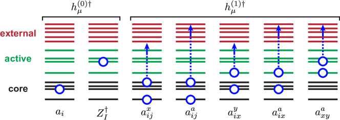
Figure 2: Schematic illustration of the ionized states produced by acting the $h_{\mu}^{(0){\dagger}}$ and $h_{\mu}^{(1){\dagger}}$ operators (Eqs. 40 and 41) on the reference state $\ket{\Psi_{0}}$. The black, green, and red energy levels correspond to core, active, and external orbitals. Empty circle represents ionization and dashed line with an arrow denotes single excitation.

2.2.3 Ionization Operator Manifolds

To determine the ionization operators $h_{\mu}^{(k){\dagger}}$ ($k=0,1$), we use the fact that these operators must satisfy two requirements:^{72, 60} (i) at the $k$th order, the particle-hole rank of $h_{\mu}^{(k){\dagger}}$ must not exceed that of $\tilde{q}_{\mu}^{(k){\dagger}}$ or $\tilde{q}_{\mu}^{(k)}$ for the forward or backward components of the propagator, respectively; (ii) $h_{\mu}^{(k){\dagger}}$ must fulfill the vacuum annihilation condition (VAC)^{75, 76, 77, 78} with respect to the reference state, i.e. $h_{\mu}^{(k)}\ket{\Psi_{0}}=0$, which ensures decoupling of the forward and backward components of the propagator in Section 2.1.^{72, 60} To obtain $h_{\mu}^{(0){\dagger}}$, we recall that $\tilde{q}_{\mu}^{(0)}=a_{p}$, where the annihilation operator can be of three different types: $a_{i}$, $a_{x}$, or $a_{a}$ (core, active, or external). Out of these three classes, only the core operator $a_{i}$ satisfies VAC with respect to $\ket{\Psi_{0}}$ ($a^{\dagger}_{i}\ket{\Psi_{0}}=0$) and, thus, can be added to $h_{\mu}^{(0){\dagger}}$. Since $\ket{\Psi_{0}}$ does not contain electrons in the active space, the external operator $a_{a}$ is redundant ($a_{a}\ket{\Psi_{0}}=0$) and cannot be included in $h_{\mu}^{(0){\dagger}}$. Although the active-space operator $a_{x}$ does not fulfill VAC ($a^{\dagger}_{x}\ket{\Psi_{0}}\neq 0$), it can be expanded⁶⁰ in the form $a_{x}=\sum_{I}Z^{\dagger}_{I}c_{I,x}$, where $Z^{\dagger}_{I}$ is a complete set of active-space eigenoperators,^{109, 110, 111} defined as:

$$Z^{\dagger}_{I} =\ket{\Psi_{I}^{N-1}}\bra{\Psi_{0}}$$ (39)

Here, $\ket{\Psi_{I}^{N-1}}$ are the CASCI states of the ionized system with $N-1$ electrons computed using the active space and one-electron basis of the reference state $\ket{\Psi_{0}}$. We note that in the context of propagator theory the configurational operators $Z^{\dagger}_{I}$ were first used by Freed and Yeager¹⁰⁹ and have two important properties: they are linearly-independent and include all types of active-only ionization operators ($a_{x}$, $a^{\dagger}_{x}a_{y}a_{z}$, $\ldots$). Incidentally, these operators also satisfy VAC with respect to $\ket{\Psi_{0}}$ and can be added to $h_{\mu}^{(0){\dagger}}$. Although we have assumed that the set of operators $Z^{\dagger}_{I}$ is complete, only a subset of these operators corresponding to CASCI states in the spectral region of interest need to be included in practice. We summarize that the MR-ADC(2) zeroth-order manifold $h_{\mu}^{(0){\dagger}}$ consists of two sets of operators:

$$\mathbf{h}^{(0){\dagger}}=\left\{a_{i};Z^{\dagger}_{I}\right\}$$ (40)

Following a similar strategy, we determine that the first-order operators $h_{\mu}^{(1){\dagger}}$ have a general form $a_{qr}^{p}\equiv a^{\dagger}_{p}a_{r}a_{q}$ and can be further divided into five classes

$$\mathbf{h}^{(1){\dagger}}=\left\{a_{ij}^{x};a_{ij}^{a};a_{ix}^{y};a_{ix}^{a};a_{xy}^{a}\right\}$$ (41)

describing ionization in the core or active spaces accompanied by core-active, active-external, or core-external single excitations, as shown in Figure 2. The all-active operators $a_{zy}^{x}$ do not appear in $\mathbf{h}^{(1){\dagger}}$, since they are already included in the $\mathbf{h}^{(0){\dagger}}$ manifold by the $Z^{\dagger}_{I}$ operators.

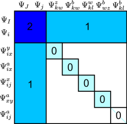
(a) $\mathbf{M}$ matrix

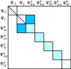
(b) $\mathbf{S}$ matrix

Figure 3: Structure of the effective Liouvillean ($\mathbf{M}$) and overlap ($\mathbf{S}$) matrices of MR-ADC(2) for photoelectron spectra. Non-zero matrix blocks are highlighted in color. A colored line represents a diagonal block. Numbers denote the perturbation order to which the effective Hamiltonian $\tilde{H}$ is approximated for each block. Wavefunctions $\Psi_{I}=Z^{\dagger}_{I}\Psi_{0}$ and $\Psi_{i}=a_{i}\Psi_{0}$ are the CASCI and core ionized states, whereas $\Psi_{qr}^{p}=a^{\dagger}_{p}a_{r}a_{q}\Psi_{0}$ are singly-excited ionized states with orbital index notation shown in Figure 1.

Figure 3 illustrates perturbative structure of the MR-ADC(2) effective Liouvillean ($\mathbf{M}$) and overlap ($\mathbf{S}$) matrices. The $\{\mathbf{h}^{(0){\dagger}}|\tilde{\mathcal{H}}^{(k)}|\mathbf{h}^{(0){\dagger}}\}$ block of the $\mathbf{M}$ matrix includes all contributions up to $k$ $=$ 2, while the coupling block $\{\mathbf{h}^{(1){\dagger}}|\tilde{\mathcal{H}}^{(k)}|\mathbf{h}^{(0){\dagger}}\}$ is evaluated to first order, as given by Section 2.2.1. In the manifold of first-order ionized states, the $\{\mathbf{h}^{(1){\dagger}}|\tilde{\mathcal{H}}^{(0)}|\mathbf{h}^{(1){\dagger}}\}$ sector is block-diagonal with non-zero elements for the $h_{\mu}^{(1){\dagger}}$ excitations from the same class (Eq. 41). Overall, the general perturbative structure of the MR-ADC(2) matrices closely resembles that of non-Dyson SR-ADC(2)^{93, 94, 95} and the two methods become equivalent in the limit of single-determinant reference wavefunction $\ket{\Psi_{0}}$.

3 Implementation

3.1 General Algorithm

In this section, we describe a general algorithm of our MR-ADC(2) implementation for complete active space (CAS) reference wavefunctions. Although in this work we always employ the ground-state CASSCF wavefunction of a neutral system as a reference, in MR-ADC other choices of reference orbitals are possible (e.g., Hartree-Fock, state-averaged, or unrestricted natural orbitals).¹¹² The main steps of the MR-ADC(2) algorithm are summarized below:

1. Choose active space, compute the reference orbitals and CAS wavefunction $\ket{\Psi_{0}}$ for the neutral system with $N$ electrons.

2. Using reference orbitals, compute the CASCI energies $E_{I}^{N-1}$ and wavefunctions $\ket{\Psi_{I}^{N-1}}$ for $N_{\mathrm{CI}}$ lowest-energy states of the ionized system with $(N-1)$ electrons.

3. Compute active-space reduced density matrices (RDMs) for the reference state $\ket{\Psi_{0}}$, transition RDMs between $\ket{\Psi_{0}}$ and ionized states $\ket{\Psi_{I}^{N-1}}$, and transition RDMs between two ionized states $\ket{\Psi_{I}^{N-1}}$.

4. Solve linear amplitude Eqs. 32 and 37 to compute $\mathbf{t^{(1)}}$ and $\mathbf{t^{(2)}}$.

5. Solve the generalized eigenvalue problem (10) to obtain ionization energies $\boldsymbol{\Omega}$.

6. Compute spectroscopic amplitudes (11) and (if necessary) spectral function (13).

As discussed in Section 2.2, the number of active-space ionized states ($N_{\mathrm{CI}}$) should be sufficiently large to include all important CASCI states in the spectral region of interest. Implementation of the algorithm outlined above requires derivation of equations for contributions to the M, T, and S matrices (Sections 2.2.1, 2.2.1 and 2.2.1). Although most of these contributions have compact expressions, matrix elements of the second-order effective Hamiltonian (e.g., $\{\mathbf{h}^{(0){\dagger}}|\tilde{\mathcal{H}}^{(2)}|\mathbf{h}^{(0){\dagger}}\}$) are very complicated containing $\sim$ 250-300 terms for each matrix block. Such algebraic complexity is a common feature of many internally-contracted multi-reference theories.^{113, 41, 31, 59, 54}

To speed up tedious derivation and implementation of MR-ADC(2), we have developed a Python program that automatically generates equations and code for arbitrary-order MR-ADC(n) approximation. Our code generator is a modified version of the SecondQuantizationAlgebra (SQA) program developed by Neuscamman and co-workers.¹¹³ We use SQA to define and normal-order all active-space creation and annihilation operators in Sections 2.2.1, 2.2.1 and 2.2.1 with respect to the physical vacuum. Next, we additionally normal-order core creation and annihilation operators relative to the Fermi vacuum and evaluate expectation values with respect to the active-space states $\ket{\Psi_{0}}$ and $\ket{\Psi_{I}^{N-1}}$. The resulting equations, written as contractions of the one- and two-electron integrals, $\mathbf{t^{(1)}}$ and $\mathbf{t^{(2)}}$ amplitudes, and RDMs, are used to generate code and can be implemented using any available tensor contraction engine. We present working equations for all matrix elements in Sections 2.2.1, 2.2.1 and 2.2.1 in the Supporting Information.

In Sections 3.2, 3.3 and 3.4, we provide more details about the solution of amplitude equations, efficient computation of terms that depend on high-order RDMs, and solution of the generalized eigenvalue problem.

3.2 Amplitude Equations

General form of the first- and second-order amplitude equations has been discussed in Section 2.2.2. Since the Dyall Hamiltonian (Eq. 4) does not contain terms that couple excitations outside of the active space, its matrix representation $\mathbf{H^{(0)}}$ (Eq. 33) is block-diagonal and the amplitude equations (32) and (37) can be solved for each block separately. Using the standard notation for classifying excitations adopted in N-electron valence perturbation theory,^{24, 25, 26} operators $\boldsymbol{\tau}$ in Section 2.2.2 are split into eight groups $\boldsymbol{\tau}^{\mathbf{[i]}}$ ($i$ $\in$ $\{0;+1;-1;+2;-2;+1^{\prime};-1^{\prime};0^{\prime}\}$), where $i$ is the number of electrons added to ($i>0$) or removed from ($i<0$) active space upon excitation. The operator classes with $i$ $\in$ $\{+1^{\prime};-1^{\prime};0^{\prime}\}$ are used to represent three coupled sets of single and semi-internal double excitations: $\boldsymbol{\tau}^{\mathbf{[+1^{\prime}]}}=\{a_{i}^{x};\ a_{ix}^{yz}\}$, $\boldsymbol{\tau}^{\mathbf{[-1^{\prime}]}}=\{a_{x}^{a};\ a_{xy}^{az}\}$, and $\boldsymbol{\tau}^{\mathbf{[0^{\prime}]}}=\{a_{i}^{a};\ a_{ix}^{ay}\}$.

Separating the $\mathbf{H^{(0)}}$, $\mathbf{t^{(1)}}$, and $\mathbf{V^{(1)}}$ matrices in Eq. 32 into blocks according to excitation classes $\boldsymbol{\tau}^{\mathbf{[i]}}$ (denoted as $\mathbf{K^{[i]}}$, $\mathbf{t^{[i](1)}}$, and $\mathbf{V^{[i](1)}}$, respectively), we express the first-order amplitude equations in the following form

$$\mathbf{K^{[i]}}\mathbf{t^{[i](1)}}=-\mathbf{V^{[i](1)}}$$ (42)

To solve Eq. 42 for each excitation class, we consider the generalized eigenvalue problem for the matrix $\mathbf{K^{[i]}}$

$$\mathbf{K^{[i]}}\mathbf{Z^{[i]}}=\mathbf{S^{[i]}}\mathbf{Z^{[i]}}\boldsymbol{\epsilon}^{\mathbf{[i]}}$$ (43)

which allows to obtain expression for the first-order amplitudes⁶⁰

$$\mathbf{t^{[i](1)}}=-(\mathbf{S^{[i]}})^{-1/2}\,\mathbf{\tilde{Z}^{[i]}}\,(\boldsymbol{\epsilon}^{\mathbf{[i]}})^{-1}\,\mathbf{\tilde{Z}^{[i]{\dagger}}}\,(\mathbf{S^{[i]}})^{-1/2}\,\mathbf{V^{[i](1)}}$$ (44)

where $K_{\mu\nu}^{[i]}=\braket{\Psi_{0}}{\tau^{[i]{\dagger}}_{\mu}(H^{(0)}-E_{0})\tau^{[i]}_{\nu}}{\Psi_{0}}$, $S^{[i]}_{\mu\nu}=\braket{\Psi_{0}}{\tau^{[i]{\dagger}}_{\mu}\tau^{[i]}_{\nu}}{\Psi_{0}}$, and $\mathbf{\tilde{Z}^{[i]}}=(\mathbf{S^{[i]}})^{1/2}\,\mathbf{Z^{[i]}}$. Computing the $\mathbf{t^{[i](1)}}$ amplitudes in Eq. 44 requires diagonalizing $\mathbf{K^{[i]}}$ and $\mathbf{S^{[i]}}$ and removing linear dependencies corresponding to eigenvectors of $\mathbf{S^{[i]}}$ with small eigenvalues. Since the matrix elements $K_{\mu\nu}^{[i]}$ and $S^{[i]}_{\mu\nu}$ are zero when the operators $\tau^{[i]{\dagger}}_{\mu}$ and $\tau^{[i]}_{\nu}$ do not share the same core and external indices, diagonalization of $\mathbf{K^{[i]}}$ and $\mathbf{S^{[i]}}$ can be performed very efficiently. For the semi-internal amplitudes $\mathbf{t^{[i](1)}}$ ($i$ $\in$ $\{+1^{\prime};-1^{\prime};0^{\prime}\}$), removing redundancies in the overlap matrix may introduce small size-consistency errors of the MR-ADC energies due to the appearance of disconnected terms in the amplitude equations that become non-zero when linear dependencies are eliminated.^{60, 114} To restore full size-consistency of the MR-ADC energies, we use the approach developed by Hanauer and Köhn¹¹⁵ that removes the disconnected terms by transforming the excitation operators $\boldsymbol{\tau}^{\mathbf{[i]}}$ ($i$ $\in$ $\{+1^{\prime};-1^{\prime};0^{\prime}\}$) to a generalized normal-ordered form. We will demonstrate size-consistency of the MR-ADC(2) ionization energies in Section 5.1.

We use Eq. 44 to compute $\mathbf{t^{[i](1)}}$ for all double ($i$ $\in$ $\{0;+1;-1;+2;-2\}$) and one class of semi-internal ($i$ $=$ $0^{\prime}$) excitations. For the $\mathbf{t^{[+1^{\prime}](1)}}$ and $\mathbf{t^{[-1^{\prime}](1)}}$ amplitudes, diagonalization of $\mathbf{K^{[+1^{\prime}]}}$ and $\mathbf{K^{[-1^{\prime}]}}$ requires the four-particle reduced density matrix (4-RDM) of the reference state $\ket{\Psi_{0}}$, which is expensive to compute and store in memory for large active spaces (see Section 3.3 for details). To avoid computation of 4-RDM, we evaluate $\mathbf{t^{[+1^{\prime}](1)}}$ and $\mathbf{t^{[-1^{\prime}](1)}}$ using imaginary-time algorithm developed in Ref. 60, which employs a Laplace transform^{116, 57} to evaluate the operator resolvent $(H^{(0)}-E_{0})^{-1}$ without explicitly constructing and inverting the $\mathbf{K^{[+1^{\prime}]}}$ and $\mathbf{K^{[-1^{\prime}]}}$ matrices.

The second-order amplitude equations (37) need to be solved only for the semi-internal amplitudes $\mathbf{t^{[+1^{\prime}](2)}}$, $\mathbf{t^{[-1^{\prime}](2)}}$, and $\mathbf{t^{[0^{\prime}](2)}}$ (Eq. 36). Among these, only $\mathbf{t^{[+1^{\prime}](2)}}$ enter equations for the M matrix, while all three sets of semi-internal amplitudes are necessary to compute the T matrix elements. The second-order amplitudes can be obtained in a similar way as their first-order counterparts $\mathbf{t^{[i](1)}}$, i.e. by expressing $\mathbf{t^{[i](2)}}$ in the form of Eq. 44 (with $\mathbf{V^{[i](1)}}$ replaced by $\mathbf{V^{[i](2)}}$ defined in Eq. 38) or using the imaginary-time algorithm. Although solving the second-order equations is straightforward, matrix elements of the perturbation operator $\mathbf{V^{[i](2)}}$ contain $\sim$ 600 terms and are rather tedious to evaluate. On the other hand, since the primary role of $\mathbf{t^{[i](2)}}$ ($i$ $\in$ $\{+1^{\prime};-1^{\prime};0^{\prime}\}$) is to describe relaxation of the orbitals, their contributions are expected to have a small effect on the results of the MR-ADC(2) method that already incorporates orbital relaxation via the first-order amplitudes $\mathbf{t^{[i](1)}}$ and ionization operators $\mathbf{h}^{(1){\dagger}}$. To test this, we considered an approximation where we neglect contributions of $\mathbf{t^{[+1^{\prime}](2)}}$ and $\mathbf{t^{[-1^{\prime}](2)}}$ and approximate $\mathbf{t^{[0^{\prime}](2)}}$ by setting $t_{ix}^{ay(2)}\approx 0$ and neglecting all terms that depend on active-space RDMs in $\mathbf{V^{[0^{\prime}](2)}}$ to obtain $t_{i}^{a(2)}$ (see the Supporting Information). The resulting amplitude equations ensure that MR-ADC(2) is equivalent to SR-ADC(2) in the single-reference limit. As demonstrated in the Supporting Information, approximating the $\mathbf{t^{(2)}}$ terms has a very small effect on the MR-ADC(2) results with errors of $\leq$ 0.005 eV and $\leq$ $3\times 10^{-4}$ in ionization energies and spectroscopic factors, respectively. For this reason, we adopted this approximation in our implementation of MR-ADC(2).

3.3 Avoiding High-Order Reduced Density Matrices

As other internally-contracted multi-reference perturbation theories, MR-ADC(2) contains terms that depend on high-order reduced density matrices (e.g., 4-RDM) in its equations. In this section, we will demonstrate that these terms can be efficiently evaluated without computing and storing 4-RDMs in memory. There are two sources of high-order RDMs in the MR-ADC(2) equations: (i) $\mathbf{t^{(1)}}$ and $\mathbf{t^{(2)}}$ amplitude equations and (ii) second-order contributions to the effective Liouvillean matrix $\mathbf{M}$. As discussed in Section 3.2, using the imaginary-time algorithm⁶⁰ allows to completely avoid computation of 4-RDM in the amplitude equations.

For the $\mathbf{M}$ matrix, 4-RDMs appear in expectation values of the second-order effective Hamiltonian $\tilde{\mathcal{H}}^{(2)}$ with respect to the reference ($\braket{\Psi_{0}}{\tilde{\mathcal{H}}^{(2)}}{\Psi_{0}}$) and ionized ($\braket{\Psi_{I}^{N-1}}{\tilde{\mathcal{H}}^{(2)}}{\Psi_{J}^{N-1}}$) wavefunctions. In particular, the latter matrix elements depend on transition 4-RDMs between all CASCI ionized states (e.g., $\braket{\Psi_{I}^{N-1}}{a^{\dagger}_{w}a^{\dagger}_{x}a^{\dagger}_{y}a^{\dagger}_{z}a_{z^{\prime}}a_{y^{\prime}}a_{x^{\prime}}a_{w^{\prime}}}{\Psi_{J}^{N-1}}$), which have a high $\mathcal{O}(N_{\mathrm{det}}N_{\mathrm{CI}}^{2}N^{8}_{\mathrm{act}})$ computational scaling, where $N_{\mathrm{det}}$ is the dimension of CAS Hilbert space, $N_{\mathrm{CI}}$ is the number of CASCI ionized states, and $N_{\mathrm{act}}$ is the number of active orbitals. To demonstrate how to avoid computation of 4-RDMs, we consider one of the contributions to the $\braket{\Psi_{I}^{N-1}}{\tilde{\mathcal{H}}^{(2)}}{\Psi_{J}^{N-1}}$ matrix elements

$$\frac{1}{8}\sum_{\begin{subarray}{c}awxyzu\\ vy^{\prime}w^{\prime}z^{\prime}\end{subarray}}v^{zw}_{xy}t^{xu}_{av}t^{ay^{\prime}}_{z^{\prime}w^{\prime}}\langle\Psi_{I}\lvert a^{\dagger}_{z}a^{\dagger}_{w}a^{\dagger}_{u}a^{\dagger}_{y^{\prime}}a_{y}a_{v}a_{w^{\prime}}a_{z^{\prime}}\rvert\Psi_{J}\rangle$$ (45)

where we use shorthand notation for the first-order amplitudes $t_{xy}^{az(1)}\equiv t_{xy}^{az}$ and CASCI states $\ket{\Psi_{I}^{N-1}}\equiv\ket{\Psi_{I}}$. Changing the order of creation and annihilation operators, we express Eq. 45 in the following form

$$-\frac{1}{8}\sum_{\begin{subarray}{c}awxyzu\\ vy^{\prime}w^{\prime}z^{\prime}\end{subarray}}v^{zw}_{xy}t^{xu}_{av}t^{ay^{\prime}}_{z^{\prime}w^{\prime}}\langle\Psi_{I}\lvert a^{\dagger}_{z}a^{\dagger}_{w}a_{y}a^{\dagger}_{u}a_{v}a^{\dagger}_{y^{\prime}}a_{w^{\prime}}a_{z^{\prime}}\rvert\Psi_{J}\rangle+\ldots$$ (46)

where the remaining terms involve contractions of transition 2- and 3-RDMs. Computing intermediate states

$$\rvert t^{J}_{a}\rangle =\frac{1}{2}\sum_{y^{\prime}w^{\prime}z^{\prime}}t^{ay^{\prime}}_{z^{\prime}w^{\prime}}a^{\dagger}_{y^{\prime}}a_{w^{\prime}}a_{z^{\prime}}\rvert\Psi_{J}\rangle$$ (47)

$$\rvert v^{I}_{x}\rangle =\frac{1}{2}\sum_{ywz}v^{xy}_{zw}a^{\dagger}_{y}a_{w}a_{z}\rvert\Psi_{I}\rangle$$ (48)

we evaluate the first term in Eq. 46 using a compact expression

$$-\frac{1}{2}\sum_{\begin{subarray}{c}axuv\end{subarray}}t^{xu}_{av}\langle v^{I}_{x}\lvert a^{\dagger}_{u}a_{v}\rvert t^{J}_{a}\rangle$$ (49)

Using Eqs. 47, 48 and 49 allows us to significantly lower the cost of computing transition 4-RDM terms from $\mathcal{O}(N_{\mathrm{det}}N_{\mathrm{CI}}^{2}N^{8}_{\mathrm{act}})$ to $\mathcal{O}(N_{\mathrm{det}}N_{\mathrm{CI}}^{2}N^{3}_{\mathrm{act}}N_{\mathrm{ext}})$, where $N_{\mathrm{ext}}$ is the number of external orbitals. We use the same technique to efficiently evaluate all 4-RDM terms that appear in the $\braket{\Psi_{I}^{N-1}}{\tilde{\mathcal{H}}^{(2)}}{\Psi_{J}^{N-1}}$ and $\braket{\Psi_{0}}{\tilde{\mathcal{H}}^{(2)}}{\Psi_{0}}$ matrix elements. We note that similar techniques have been used to avoid computation of 4-RDM in implementations of complete active space second-order perturbation theory (CASPT2) and NEVPT2 in combination with matrix product state wavefunctions.^{116, 117, 57}

The $\mathbf{M}$ matrix elements also depend on transition RDMs of the form $\braket{\Psi_{0}}{a^{\dagger}_{w}a^{\dagger}_{x}a^{\dagger}_{y}a^{\dagger}_{z}a_{z^{\prime}}a_{y^{\prime}}a_{x^{\prime}}}{\Psi_{I}^{N-1}}$, which we denote as 3.5-RDMs. These RDMs contribute to the second-order matrix elements $\braket{\Psi_{0}}{a^{\dagger}_{i}\tilde{\mathcal{H}}^{(2)}}{\Psi_{I}^{N-1}}$, as well as some elements of the first-order off-diagonal blocks $\{\mathbf{h}^{(1){\dagger}}|\tilde{\mathcal{H}}^{(1)}|\mathbf{h}^{(0){\dagger}}\}$ and $\{\mathbf{h}^{(0){\dagger}}|\tilde{\mathcal{H}}^{(1)}|\mathbf{h}^{(1){\dagger}}\}$ in Section 2.2.1. For example, a 3.5-RDM contribution to $\braket{\Psi_{0}}{a^{\dagger}_{i}\tilde{\mathcal{H}}^{(2)}}{\Psi_{I}^{N-1}}$ has a form

$$\frac{1}{8}\sum_{\begin{subarray}{c}awxyz\\ uvu^{\prime}w^{\prime}\end{subarray}}v^{xy}_{zw}t^{iz}_{au}t^{vu^{\prime}}_{aw^{\prime}}\langle\Psi_{0}\lvert a^{\dagger}_{w}a^{\dagger}_{u}a^{\dagger}_{v}a^{\dagger}_{u^{\prime}}a_{y}a_{x}a_{w^{\prime}}\rvert\Psi_{I}\rangle$$ (50)

To evaluate this term, we reorder creation and annihilation operators, contract $v^{xy}_{zw}$ and $t^{vu^{\prime}}_{aw^{\prime}}$ with $a^{\dagger}_{x}a^{\dagger}_{y}a_{w}\rvert\Psi_{0}\rangle$ and $a^{\dagger}_{v}a^{\dagger}_{u^{\prime}}a_{w^{\prime}}\rvert\Psi_{I}\rangle$ to form intermediate states ($\rvert v^{z}\rangle$ and $\rvert t_{I}^{a}\rangle$), and contract $t^{iz}_{au}$ with their overlap matrix element ($\langle v^{z}\lvert a^{\dagger}_{u}\rvert t^{a}_{I}\rangle$). As in the case of 4-RDM, using intermediate states allows to completely avoid computation and storage of 3.5-RDMs for all terms of the $\mathbf{M}$ matrix, lowering computational scaling from $\mathcal{O}(N_{\mathrm{det}}N_{\mathrm{CI}}N^{7}_{\mathrm{act}})$ to $\mathcal{O}(N_{\mathrm{det}}N_{\mathrm{CI}}N^{2}_{\mathrm{act}}N_{\mathrm{ext}})$.

Combining efficient algorithms for the solution of amplitude equations and evaluation of high-order RDM terms, our MR-ADC(2) implementation has $\mathcal{O}(N_{\mathrm{det}}N^{2}_{\mathrm{CI}}N^{6}_{\mathrm{act}})$ computational scaling, which is significantly lower than the $\mathcal{O}(N_{\mathrm{det}}N^{8}_{\mathrm{act}})$ scaling of the conventional multi-reference perturbation theories (e.g., CASPT2 or NEVPT2) with the number of active orbitals. Although the scaling of our current MR-ADC(2) algorithm originates from computing transition 3-RDMs ($\braket{\Psi_{I}^{N-1}}{a^{\dagger}_{w}a^{\dagger}_{x}a^{\dagger}_{y}a_{y^{\prime}}a_{x^{\prime}}a_{w^{\prime}}}{\Psi_{J}^{N-1}}$) for all ionized states, we note that using intermediate states the computational cost can be further lowered to $\mathcal{O}(N_{\mathrm{det}}N_{\mathrm{CI}}N^{6}_{\mathrm{act}})$. We did not take advantage of it in our present implementation.

3.4 Solution of the Generalized Eigenvalue Problem

Finally, we briefly discuss solution of the MR-ADC(2) generalized eigenvalue problem in Eq. 10. Since the $\mathbf{M}$ and $\mathbf{S}$ matrices are computed in the non-orthogonal basis of internally-contracted ionized states, we transform the eigenvalue equation to the symmetrically-orthogonalized form

$$\mathbf{\tilde{M}}\mathbf{\tilde{Y}}=\mathbf{\tilde{Y}}\boldsymbol{\Omega}$$ (51)

where $\mathbf{\tilde{M}}=\mathbf{S}^{-1/2}\mathbf{M}\mathbf{S}^{-1/2}$ and $\mathbf{\tilde{Y}}=\mathbf{S}^{1/2}\mathbf{Y}$. Here, the overlap matrix $\mathbf{S}$ contains four non-diagonal blocks corresponding to ionized states $\ket{\Psi_{\mu}}=\{a_{ij}^{x}\ket{\Psi_{0}}$; $a_{ix}^{a}\ket{\Psi_{0}}$; $a_{xy}^{a}\ket{\Psi_{0}}$; $a_{i}\ket{\Psi_{0}}$; $a_{ix}^{y}\ket{\Psi_{0}}\}$ (Figure 3b). Conveniently, the $\mathbf{S}^{-1/2}$ matrix can be constructed together with the $(\mathbf{S^{[i]}})^{-1/2}$ matrices used for solution of the amplitude equations (Section 3.2). As an example, we consider non-zero elements of $\mathbf{S}$ for $a_{ij}^{x}\ket{\Psi_{0}}$ that have the form $S_{ijx,ijy}=\braket{\Psi_{0}}{a_{y}^{ij}a_{ij}^{x}}{\Psi_{0}}=\braket{\Psi_{0}}{a_{y}a^{\dagger}_{x}}{\Psi_{0}}$. These elements are equal to the $\mathbf{S^{[+1]}}$ matrix elements $S_{ijay,ijax}^{[+1]}=\braket{\Psi_{0}}{a_{ay}^{ij}a_{ij}^{ax}}{\Psi_{0}}=\braket{\Psi_{0}}{a_{y}a^{\dagger}_{x}}{\Psi_{0}}$. Thus, by diagonalizing the density matrix $\braket{\Psi_{0}}{a_{y}a^{\dagger}_{x}}{\Psi_{0}}$ and removing linearly-dependent eigenvectors corresponding to small eigenvalues ($<$ $\eta_{d}$, where $\eta_{d}$ is a user-defined truncation parameter), we simultaneously obtain elements of $(\mathbf{S^{[+1]}})^{-1/2}$ and $\mathbf{S}^{-1/2}$ for the $a_{ij}^{x}\ket{\Psi_{0}}$ ionized wavefunctions. Similarly, we construct $(\mathbf{S^{[-1]}})^{-1/2}$ and $(\mathbf{S^{[-2]}})^{-1/2}$ together with $\mathbf{S}^{-1/2}$ for $a_{ix}^{a}\ket{\Psi_{0}}$ and $a_{xy}^{a}\ket{\Psi_{0}}$, respectively.

For the $a_{ij}^{x}\ket{\Psi_{0}}$, $a_{ix}^{a}\ket{\Psi_{0}}$, and $a_{xy}^{a}\ket{\Psi_{0}}$ states, numerical instabilities due to linear dependencies are completely eliminated when using small truncation parameters ($\eta_{d}$ $\sim$ $10^{-10}$). Except for very small active spaces ($N_{\mathrm{act}}<6$), orthogonalization of these ionized states does not require discarding any eigenvectors of the overlap matrix. The zeroth-order $a_{i}\ket{\Psi_{0}}$ and first-order $a_{ix}^{y}\ket{\Psi_{0}}$ ionized states exhibit much stronger linear dependencies in their overlap matrix. To remove these linear dependencies, we project out $a_{i}\ket{\Psi_{0}}$ from $a_{ix}^{y}\ket{\Psi_{0}}$ using the projection approach developed by Hanauer and Köhn¹¹⁴ and subsequently orthogonalize $a_{ix}^{y}\ket{\Psi_{0}}$ between each other. Importantly, this ensures that the zeroth-order states $a_{i}\ket{\Psi_{0}}$, which are already orthogonal, are not affected by removing redundancies in the first-order $a_{ix}^{y}\ket{\Psi_{0}}$ ionization manifold. To discard linearly-dependent eigenvectors of the $a_{ix}^{y}\ket{\Psi_{0}}$ overlap matrix, we use a larger truncation parameter ($\eta_{s}$ $\sim$ $10^{-6}$) than the one used for other ionized states ($\eta_{d}$).

We solve the eigenvalue problem (51) using a multi-root implementation of the Davidson algorithm,^{118, 119} which avoids storing the full M and S matrices, significantly reducing the memory requirements. Since the second-order block $\{\mathbf{h}^{(0){\dagger}}|\tilde{\mathcal{H}}^{(2)}|\mathbf{h}^{(0){\dagger}}\}$ of M is small (with $(N_{\mathrm{CI}}+N_{\mathrm{act}})^{2}$ elements) and its computation is the most time-consuming step of the MR-ADC(2) implementation, we precompute this block, store it memory, and use it for the efficient evaluation of matrix-vector products in the Davidson procedure.

4 Computational Details

We implemented MR-ADC(2) for photoelectron spectra in our pilot code Prism, which was interfaced with Pyscf¹²⁰ to obtain integrals and CASCI/CASSCF reference wavefunctions. Our implementation follows the general algorithm outlined in Section 3.1. All MR-ADC(2) computations used the CASSCF reference wavefunctions with molecular orbitals optimized for the ground electronic state of each (neutral) system. To remove linear dependencies in the solution of amplitude equations and generalized eigenvalue problem, we truncated eigenvectors of the overlap matrices using two parameters: $\eta_{s}$ = $10^{-6}$ and $\eta_{d}$ = $10^{-10}$ (see Section 3.4 for details). The $\eta_{s}$ parameter was used to orthogonalize the $a_{ix}^{y}\ket{\Psi_{0}}$ ionized states and to compute the semi-internal $\mathbf{t^{[i](1)}}$ ($i$ $\in$ $\{+1^{\prime};-1^{\prime};0^{\prime}\}$) amplitudes (Section 3.2), while $\eta_{d}$ was employed for other amplitudes and ionized states. To efficiently compute $\mathbf{t^{[+1^{\prime}](1)}}$ and $\mathbf{t^{[-1^{\prime}](1)}}$, our implementation used imaginary-time algorithm,^{60, 116, 57} where propagation in imaginary time was performed using the embedded Runge-Kutta method that automatically determines time step based on the accuracy parameter $\Delta_{it}$.¹²¹ In all computations, we used $\Delta_{it}$ = $10^{-7}$ $E_{\mathrm{h}}$, which allows to obtain very accurate amplitudes and reference NEVPT2 correlation energy. All MR-ADC(2) results were converged with respect to the number of CASCI ionized states ($N_{\mathrm{CI}}$). For most of the systems employed in this study, using $N_{\mathrm{CI}}$ = 20 was enough to obtain well-converged results.

We benchmarked the accuracy of MR-ADC(2) for a set of small molecules (HF, F2, CO, N2, H2O, CS, H2CO, and C2H4), carbon dimer (C2), and hydrogen chains (H10 and H30). For small molecules, equilibrium and stretched geometries were considered. The equilibrium structures were taken from Ref. 94. For diatomic molecules, the stretched geometries were obtained by increasing the bond length by a factor of two. For the H2O, H2CO, and C2H4 stretched geometries, we doubled the O-H, C-O, and C-C bond distances, respectively. The C-C bond length in C2 was set to 1.2425 Å, which is very close to its equilibrium geometry. Unless noted otherwise, all computations employed the aug-cc-pVDZ basis set.¹²² For H2CO and C2H4, the cc-pVDZ basis set was used for the hydrogen atoms, as employed in Ref. 94. We denote active spaces used in CASCI/CASSCF as ($n$e, $m$o), where $n$ is the number of active electrons and $m$ is the number of active orbitals. Active spaces of small molecules included 10 orbitals with $n$ = 8, 14, 10, 10, 8, 10, 12, and 10 active electrons for HF, F2, CO, N2, H2O, CS, H2CO, and C2H4, respectively. For C2, the (8e, 12o) active space was used. For the hydrogen chains, we employed the (10e, 10o) active space.

The MR-ADC(2) results were compared to results of single-reference non-Dyson ADC methods (SR-ADC(2) and SR-ADC(3)),^{93, 94, 95} equation-of-motion coupled cluster theory for ionization energies with single and double excitations (EOM-CCSD),^{123, 124, 83} quasi-degenerate strongly-contracted second-order N-electron valence perturbation theory (QD-NEVPT2),²⁶ as well as full configuration interaction (FCI). All methods employed the same geometries and basis sets as those used for MR-ADC(2). SR-ADC(2) and SR-ADC(3) were implemented by our group as a module in the development version of Pyscf. The FCI results were computed using the semistochastic heat-bath configuration interaction algorithm (SHCI) implemented in the Dice program.^{12, 13, 14} The SHCI electronic energies were extrapolated using a linear fit according to procedure described in Ref. 14. We estimate that errors of the computed SHCI energy differences relative to FCI do not exceed 0.03 eV. For H2CO and C2H4, the $1s$ atomic orbitals of carbon and oxygen were not correlated in the SHCI computations. For all other methods, all electrons were correlated in all computations. The EOM-CCSD and QD-NEVPT2 results were obtained using Q-Chem¹²⁵ and Orca,¹²⁶ respectively. For the ground state of each neutral system, QD-NEVPT2 used the same active spaces and CASSCF reference wavefunctions as those employed in MR-ADC(2). The QD-NEVPT2 computations of ionized states used the state-averaged CASSCF reference wavefunctions, where state-averaging included four electronic states for each abelian subgroup irreducible representation of the full symmetry point group.

Intensities of photoelectron transitions were characterized by computing spectroscopic factors

$$P_{\mu}=\sum_{p}|X_{p,\mu}|^{2}$$ (52)

where $X_{p,\mu}$ are elements of the spectroscopic amplitude matrix $\mathbf{X}_{\pm}$ defined in Eq. 11. Spectroscopic factors in Eq. 52 correspond to intensities of photoelectron transitions under the approximation that only single-electron detachment contributes to the spectrum. More rigorous simulation of photoelectron intensities require computation of Dyson orbitals with explicit treatment of the wavefunction of injected free electron and will be one of the subjects of our future work.¹²⁷

5 Results

5.1 Size-Consistency of Energies and Properties

Table 1: Size-consistency errors of the MR-ADC(2) ionization energies ($\Delta\Omega$, eV) and spectroscopic factors ($\Delta P$) for the (H2O)2 and (HF)2 systems composed of two identical monomers separated by 10000 Å (aug-cc-pVDZ basis set). For H2O, $r_{e}$ = $r$(O-H) = 1.0 Å and $\angle$(H–O–H) = 104.5^∘. For HF, $r_{e}$ = 0.917 Å. The (4e, 4o) and (6e, 5o) active spaces were used for the H2O and HF monomer CASSCF reference wavefunctions. For dimers, (8e, 8o) and (12e, 10o) active spaces were used, respectively. The number of CASCI ionized states was set to 10 and 20, for monomers and dimers, respectively.

System	State	$\Delta\Omega$	$\Delta P$
(H2O)2 ($r_{e}$)	$1b_{1}$	$-$2.4 $\times$ $10^{-5}$	6.0 $\times$ $10^{-8}$
	$3a_{1}$	9.4 $\times$ $10^{-6}$	$-$2.7 $\times$ $10^{-7}$
	$1b_{2}$	2.8 $\times$ $10^{-6}$	2.5 $\times$ $10^{-7}$
(H2O)2 ($2r_{e}$)	$1b_{1}$	$-$1.3 $\times$ $10^{-5}$	3.4 $\times$ $10^{-7}$
	$3a_{1}$	1.5 $\times$ $10^{-5}$	2.3 $\times$ $10^{-6}$
	$1b_{2}$	1.3 $\times$ $10^{-5}$	1.8 $\times$ $10^{-6}$
(HF)2 ($r_{e}$)	$1\pi$	1.2 $\times$ $10^{-4}$	$-$1.0 $\times$ $10^{-6}$
	$3\sigma$	5.4 $\times$ $10^{-5}$	2.4 $\times$ $10^{-6}$
(HF)2 ($2r_{e}$)	$1\pi$	1.0 $\times$ $10^{-4}$	$-$4.5 $\times$ $10^{-6}$
	$3\sigma$	5.9 $\times$ $10^{-5}$	$-$9.1 $\times$ $10^{-7}$

We begin by testing size-consistency of the MR-ADC(2) ionization energies and spectroscopic factors. As for single-reference ADC, the MR-ADC equations are fully connected, which guarantees size-consistency of the MR-ADC energies and transition properties. In practice, however, removing redundancies in the overlap matrix during the solution of the MR-ADC amplitude equations may result in small size-consistency errors.⁶⁰ As we discussed in Section 3.2, in this work we employ a technique developed by Hanauer and Köhn that restores size-consistency of the MR-ADC results. Table 1 shows deviations from size-consistency of the MR-ADC(2) ionization energies ($\Delta\Omega$) and spectroscopic factors ($\Delta P$) for the (H2O)2 and (HF)2 systems, each composed of two noninteracting monomers with near-equilibrium ($r_{e}$) and stretched geometries ($2\times r_{e}$). The computed size-consistency errors are very small: $\Delta\Omega$ $\sim$ $10^{-5}$ eV and $\Delta P$ $\sim$ $10^{-6}$ on average, with the largest errors of $\Delta\Omega$ = 1.2 $\times$ $10^{-4}$ eV and $\Delta P$ = $-$4.5 $\times$ $10^{-6}$. These remaining errors originate from a finite time step used in the imaginary-time algorithm for solving the semi-internal amplitude equations and become increasingly smaller with a tighter $\Delta_{it}$ parameter (see Section 4 for details). Overall, our numerical results demonstrate size-consistency of the MR-ADC(2) results in the present implementation.

5.2 Small Molecules

Table 2: Computed vertical ionization energies ($\Omega$, eV) and spectroscopic factors ($P$) of molecules with equilibrium geometries. See Section 4 for active spaces used in the reference CASSCF computations, structural parameters, and basis sets. Also shown are mean absolute errors ($\Delta_{\mathrm{MAE}}$) and standard deviations ($\Delta_{\mathrm{STD}}$) of the results, relative to FCI.

System	State	SR-ADC(2)		SR-ADC(3)		SR-ADC(3+)a		MR-ADC(2)		EOM-CCSD	QD-NEVPT2	FCI
		$\Omega$	$P$	$\Omega$	$P$	$\Omega$	$P$	$\Omega$	$P$	$\Omega$	$\Omega$	$\Omega$
HF	$1\pi$	14.41	0.89	16.79	0.93	16.41	0.93	16.35	0.93	15.85	16.00	16.07
	$3\sigma$	18.69	0.90	20.65	0.94	20.30	0.94	20.38	0.94	19.88	20.04	20.06
F2	$1\pi_{g}$	13.90	0.87	16.03	0.89	15.87	0.90	16.55	0.88	15.40	15.38	15.64
	$1\pi_{u}$	17.06	0.84	19.25	0.75	19.11	0.81	19.86	0.80	18.77	18.58	18.83
	$3\sigma_{g}$	20.25	0.89	21.26	0.89	21.01	0.88	22.08	0.87	21.16	20.88	21.15
CO	$5\sigma$	13.78	0.91	13.57	0.90	13.80	0.89	14.07	0.92	13.99	13.53	13.74
	$1\pi$	16.24	0.89	17.16	0.90	16.88	0.90	17.38	0.90	16.93	16.75	16.90
	$4\sigma$	18.28	0.85	20.46	0.76	20.10	0.79	20.15	0.85	19.67	19.48	19.56
N2	$3\sigma_{g}$	14.79	0.88	15.42	0.91	15.60	0.91	15.76	0.91	15.43	15.21	15.30
	$1\pi_{u}$	16.98	0.91	16.60	0.92	16.77	0.92	17.33	0.92	17.11	16.75	16.83
	$2\sigma_{u}$	17.96	0.85	18.79	0.82	18.93	0.82	19.00	0.83	18.71	18.44	18.50
H2O	$1b_{1}$	11.23	0.89	12.99	0.92	12.78	0.92	12.74	0.93	12.38	12.55	12.53
	$3a_{1}$	13.53	0.89	15.28	0.92	15.08	0.93	15.07	0.93	14.66	14.85	14.81
	$1b_{2}$	17.95	0.90	19.34	0.93	19.16	0.93	19.28	0.94	18.89	19.05	18.98
CS	$7\sigma$	10.99	0.86	10.99	0.85	11.33	0.85	11.59	0.85	11.36	10.95	11.13
	$2\pi$	12.84	0.91	12.67	0.90	12.66	0.90	13.43	0.91	12.94	12.74	12.83
	$6\sigma$	16.88	0.85	15.53	0.18	15.51	0.19	16.83	0.40	17.02	15.83	15.88
H2CO	$2b_{2}$	9.46	0.87	11.11	0.91	10.87	0.91	11.23	0.92	10.62	10.28	10.72
	$1b_{1}$	13.73	0.88	14.54	0.88	14.30	0.88	15.14	0.90	14.47	14.07	14.48
	$5a_{1}$	14.62	0.86	16.61	0.90	16.20	0.90	16.70	0.90	15.95	15.64	16.01
	$1b_{2}$	16.67	0.88	17.04	0.69	17.32	0.65	17.76	0.88	17.21	16.50	16.86
C2H4	$1b_{1u}$	10.14	0.91	10.47	0.91	10.46	0.91	11.01	0.90	10.58	10.41	10.58
	$1b_{1g}$	12.79	0.91	13.22	0.91	13.19	0.91	13.75	0.92	13.22	13.05	13.21
	$3a_{g}$	13.78	0.89	14.34	0.91	14.36	0.91	14.74	0.89	14.31	14.12	14.25
	$1b_{2u}$	16.13	0.87	16.50	0.74	16.49	0.79	17.10	0.84	16.61	16.35	16.45
$\Delta_{\mathrm{MAE}}$		0.83		0.30		0.21		0.56		0.17	0.17
$\Delta_{\mathrm{STD}}$		0.68		0.32		0.22		0.23		0.28	0.14

• Non-Dyson SR-ADC(3) incorporating high-order self-energy corrections from Ref. 94.

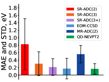
(a)

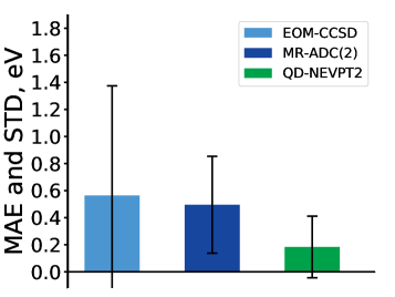
(b)

Figure 4: Mean absolute errors (MAE, eV) and standard deviations from the mean signed error (STD, eV) for vertical ionization energies of molecules with (a) equilibrium and (b) stretched geometries computed using six methods, relative to FCI (aug-cc-pVDZ basis set). The MAE value is represented as a height of each colored box, while the STD value is depicted as a radius of the black vertical bar.

In this section, we benchmark the MR-ADC(2) accuracy for predicting ionization energies of small molecules. Table 2 compares vertical ionization energies ($\Omega$) and spectroscopic factors ($P$) of MR-ADC(2) with those obtained by single-reference non-Dyson ADC methods (SR-ADC), equation-of-motion coupled cluster theory with single and double excitations (EOM-CCSD), quasi-degenerate NEVPT2 (QD-NEVPT2), and full configuration interaction (FCI) for a set of eight molecules near their equilibrium geometries (see Section 4 for computational details). In addition to strict second- and third-order SR-ADC (SR-ADC(2) and SR-ADC(3)), Table 2 also presents results of SR-ADC(3) incorporating high-order self-energy corrections, reported in Ref. 94, which we denote as SR-ADC(3+). Out of six approximate methods, the best agreement with FCI is shown by SR-ADC(3+), EOM-CCSD, and QD-NEVPT2. These three methods produce similar mean absolute errors in vertical ionization energies ($\Delta_{\mathrm{MAE}}$ $\sim$ 0.2 eV) with standard deviations from the mean signed error ($\Delta_{\mathrm{STD}}$) ranging from $\sim$ 0.15 to 0.3 eV, as illustrated in Figure 4a. The MR-ADC(2) method shows a similar $\Delta_{\mathrm{STD}}$ error (0.23 eV), but a larger $\Delta_{\mathrm{MAE}}$ error (0.56 eV), which is lower than $\Delta_{\mathrm{MAE}}$ of SR-ADC(2) (0.83 eV), but higher than that of SR-ADC(3) (0.30 eV), indicating that including high-order effects in MR-ADC(2) improves its accuracy relative to SR-ADC(2). For all systems, the MR-ADC(2) ionization energies systematically overestimate energies computed using FCI, showing a good agreement with FCI for energy spacings between electronic states of the ionized systems ($\Delta_{\mathrm{MAE}}$ of 0.11 eV and $\Delta_{\mathrm{STD}}$ of 0.10 eV). The QD-NEVPT2 method shows the best agreement with FCI for energy spacings ($\Delta_{\mathrm{MAE}}$ and $\Delta_{\mathrm{STD}}$ of 0.03 eV), while EOM-CCSD shows larger errors compared to MR-ADC(2) ($\Delta_{\mathrm{MAE}}$ = 0.16 eV, $\Delta_{\mathrm{STD}}$ = 0.27 eV). The MR-ADC(2) spectroscopic factors agree well with those computed using SR-ADC(3) and SR-ADC(3+), with two exceptions observed for the $6\sigma$ state of CS and the $1b_{2}$ state of H2CO. In these cases, the computed spectroscopic factors vary significantly depending on the order of the ADC approximation, suggesting that properties of these photoelectron transitions are significantly affected by electron correlation effects.

Table 3: Computed vertical ionization energies ($\Omega$, eV) and spectroscopic factors ($P$) of molecules with stretched geometries. See Section 4 for active spaces used in the reference CASSCF computations, structural parameters, and basis sets. Also shown are mean absolute errors ($\Delta_{\mathrm{MAE}}$) and standard deviations ($\Delta_{\mathrm{STD}}$) of the results, relative to FCI.

System	State	SR-ADC(2)		SR-ADC(3)		MR-ADC(2)		EOM-CCSD	QD-NEVPT2	FCI
		$\Omega$	$P$	$\Omega$	$P$	$\Omega$	$P$	$\Omega$	$\Omega$
HF	$1\pi$	9.84	0.77	16.15	0.84	13.86	0.60	13.67	13.61	13.65
	$3\sigma$	13.30	0.84	14.68	0.76	14.98	0.73	14.76	14.83	14.84
F2	$1\pi_{g}$	10.63	0.64	17.55	0.88	18.12	0.74	16.86	16.81	17.13
	$1\pi_{u}$	10.66	0.64	17.69	0.89	18.16	0.82	16.95	16.87	17.19
N2	$3\sigma_{g}$	15.70	0.63	$-$2.60	1.69	14.00	0.69	14.36	13.06	13.38
	$1\pi_{u}$	17.50	0.55	$-$5.24	2.16	14.17	0.51	14.77	13.21	13.49
H2O	$1b_{1}$	6.53	0.71	12.24	0.66	11.31	0.64	10.65	10.99	11.07
	$3a_{1}$	10.49	0.75	12.78	0.67	13.22	0.67	12.69	12.99	13.02
	$1b_{2}$	11.18	0.75	13.01	0.72	13.78	0.71	13.26	13.53	13.56
H2CO	$2b_{2}$	10.65	0.85	8.31	0.21	11.51	0.39	9.85	10.24	10.37
	$1b_{1}$	10.69	0.86	8.35	0.22	11.21	0.48	9.66	10.38	10.55
	$5a_{1}$	10.60	0.91	10.97	0.88	13.16	0.57	10.97	12.32	13.16
C2H4	$1b_{1u}$	9.37	0.76	6.87	0.83	9.69	0.53	9.41	9.26	9.25
	$3a_{g}$	11.38	0.79	8.74	0.91	11.36	0.73	11.17	10.94	10.93
$\Delta_{\mathrm{MAE}}$		2.70		3.66		0.50		0.56	0.18
$\Delta_{\mathrm{STD}}$		3.10		6.28		0.36		0.81	0.23

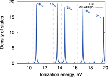
(a)

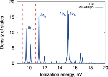
(b)

Figure 5: Simulated photoelectron spectrum of ethylene for equilibrium (a) and stretched (b) geometries computed using the MR-ADC(2) method by broadening peaks centered at vertical ionization energies with a half width of 0.03 eV (aug-cc-pVDZ basis set). Vertical dashed lines indicate FCI ionization energies for main peaks. See Tables 2 and 3 for the MR-ADC(2) and FCI data.

To assess performance of MR-ADC(2) when strong correlation is important, we computed its ionization energies and spectroscopic factors for molecules with stretched geometries, where at least one of the bonds is elongated by a factor of two (see Section 4 for details). The MR-ADC(2) results are shown in Table 3, along with those computed using SR-ADC(2), SR-ADC(3), EOM-CCSD, QD-NEVPT2, and FCI. Due to the difficulty of obtaining the FCI energies, we show results only for a few lowest-energy transitions of six molecules. Importance of strong electron correlation for these non-equilibrium geometries is demonstrated by the poor performance of SR-ADC(2) and SR-ADC(3), which show very large deviations from the FCI reference values with $\Delta_{\mathrm{MAE}}$ $>$ 2.5 eV and $\Delta_{\mathrm{STD}}$ $>$ 3 eV. Although SR-ADC(3) shows moderate $\sim$ 0.5 eV errors for single-bond stretching in HF and F2, these errors drastically increase when multiple bonds are elongated, leading to unphysical values of ionization energies that significantly underestimate the FCI results. EOM-CCSD significantly improves prediction of ionization energies over SR-ADC(2) and SR-ADC(3), but still exhibits large errors ($\Delta_{\mathrm{MAE}}$ = 0.56 and $\Delta_{\mathrm{STD}}$ = 0.81 eV, Figure 4b). MR-ADC(2) shows performance similar to that for equilibrium geometries (Table 2), with $\Delta_{\mathrm{MAE}}$ (0.50 eV) and $\Delta_{\mathrm{STD}}$ (0.36 eV) smaller than the corresponding errors for the single-reference methods. The best agreement with FCI is again shown by QD-NEVPT2 with $\Delta_{\mathrm{MAE}}$ = 0.18 eV and $\Delta_{\mathrm{STD}}$ = 0.23 eV. As for the equilibrium geometries, the MR-ADC(2) ionization energies for stretched geometries are systematically overestimated relative to FCI, reproducing energy spacings between ionized states within 0.1 eV for all systems except H2CO, where $\sim$ 0.5 eV errors are observed. QD-NEVPT2 shows a similar performance to MR-ADC(2) for energy spacings with a large error of $\sim$ 0.7 eV for the difference of the $1b_{1}$ and $5a_{1}$ ionization energies of H2CO.

Table 4: Vertical ionization energies ($\Omega$, eV) and spectroscopic factors ($P$) of carbon dimer with $r$(C-C) = 1.2425 Å computed using the aug-cc-pVDZ basis set. For MR-ADC(2) and QD-NEVPT2, the CASSCF reference wavefunction was computed using the (8e, 12o) active space.

Configuration	State	SR-ADC(3)		MR-ADC(2)		QD-NEVPT2	FCI
		$\Omega$	$P$	$\Omega$	$P$	$\Omega$	$\Omega$
$(2\sigma_{u})^{2}(1\pi_{u})^{3}(3\sigma_{g})^{0}$	$1^{2}\Pi_{u}$	11.69	0.9215	12.50	0.8986	12.28	12.34
$(2\sigma_{u})^{2}(1\pi_{u})^{2}(3\sigma_{g})^{1}$	$1^{2}\Delta_{g}$	11.17	0.0002	14.31	0.0002	13.92	13.94
$(2\sigma_{u})^{2}(1\pi_{u})^{2}(3\sigma_{g})^{1}$	$1^{2}\Sigma_{g}^{-}$	a	a	14.55	0.0000	14.12	14.15
$(2\sigma_{u})^{2}(1\pi_{u})^{2}(3\sigma_{g})^{1}$	$1^{2}\Sigma_{g}^{+}$	11.43	0.0004	14.60	0.0047	14.26	14.29
$(2\sigma_{u})^{1}(1\pi_{u})^{4}(3\sigma_{g})^{0}$	$1^{2}\Sigma_{u}^{+}$	13.95	0.8738	15.33	0.7190	15.07	15.09
$(2\sigma_{u})^{2}(1\pi_{u})^{1}(3\sigma_{g})^{2}$	$2^{2}\Pi_{u}$	a	a	14.77	0.0183	15.35	15.43

• State is absent in SR-ADC(3).

An important advantage of MR-ADC(2) over conventional multi-reference perturbation theories (such as QD-NEVPT2) is that it provides efficient access to spectroscopic properties. We demonstrate this by computing the photoelectron spectrum of C2H4 at equilibrium and stretched geometries in the range between 8.5 and 20 eV, shown in Figure 5. The spectrum at equilibrium geometry exhibits five very intense well-separated peaks corresponding to vertical ionizations in five highest occupied molecular orbitals. All of the computed peaks are systematically shifted by $\sim$ 0.5 eV relative to FCI. The computed spacings between the main peaks are in a good agreement with FCI (Table 2), as well as experimental photoelectron spectrum.¹²⁸ At the stretched geometry, the MR-ADC(2) spectrum shows four main peaks with significantly decreased intensities, along with several satellite peaks originating from shake-up transitions that involve ionization and simultaneous excitation in the valence orbitals.

5.3 Carbon Dimer

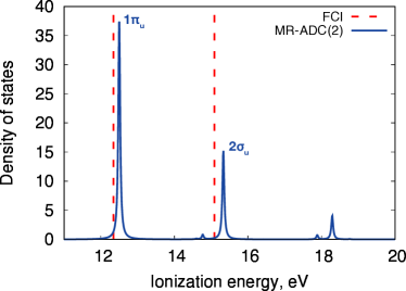
Figure 6: Simulated photoelectron spectrum of carbon dimer for $r$(C-C) = 1.2425 Å computed using the MR-ADC(2) method by broadening peaks centered at vertical ionization energies with a half width of 0.03 eV (aug-cc-pVDZ basis set). Vertical dashed lines indicate FCI ionization energies for the main peaks corresponding to the $1^{2}\Pi_{u}$ and $1^{2}\Sigma_{u}^{+}$ states of C2+ (Table 4).

Next, we investigate performance of MR-ADC(2) for simulating photoelectron spectrum of C2, which is a challenging test for ab initio methods, since electronic states of both C2 and C2+ require very accurate description of static and dynamic correlation.^{129, 130, 131, 132, 133, 14, 134, 135, 136, 137, 138, 139} Table 4 compares results of SR-ADC(3), MR-ADC(2), and QD-NEVPT2 with those from FCI. The MR-ADC(2) photoelectron spectrum, shown in Figure 6, exhibits two very intense peaks for ionizations in the $1\pi_{u}$ and $2\sigma_{u}$ orbitals, corresponding to the $1^{2}\Pi_{u}$ and $1^{2}\Sigma_{u}^{+}$ electronic states of C2+, respectively. For both peaks, MR-ADC(2) is in a good agreement with FCI, showing errors in vertical ionization energies (0.16 and 0.24 eV) within $\Delta_{\mathrm{MAE}}$ and $\Delta_{\mathrm{STD}}$ of small molecules computed in Section 5.2. The MR-ADC(2) results show significant improvement over SR-ADC(3), which underestimates the $1\pi_{u}$ and $2\sigma_{u}$ ionization energies from FCI by 0.65 and 1.14 eV, respectively, indicating that description of multi-reference effects is important for these ionization processes. The best agreement with FCI is demonstrated by QD-NEVPT2, with errors smaller than 0.1 eV.

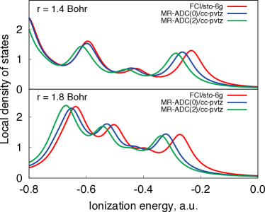
(a)

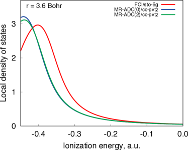
(b)

Figure 7: Local density of states (LDOS) for the equally-spaced H10 chain with $r$(H-H) = 1.4, 1.8, and 3.6 $a_{0}$ computed using three methods with 0.05 $E_{\mathrm{h}}$ broadening. LDOS was computed at the central hydrogen atom. The MR-ADC reference CASSCF wavefunction used the (10e, 10o) active space.

In addition to the intense peaks, the C2 photoelectron spectrum also exhibits several much weaker (satellite) peaks, which involve ionization in the $1\pi_{u}$ orbital accompanied by single and double $(1\pi_{u})^{3}$ $\rightarrow$ $(3\sigma_{g})^{0}$ excitations (Table 4). Out of four satellite transitions, only two are predicted by SR-ADC(3), with large errors ($>$ 2 eV). For the singly-excited shake-up states of C2+ ($1^{2}\Delta_{g}$, $1^{2}\Sigma_{g}^{-}$, and $1^{2}\Sigma_{g}^{+}$), the largest MR-ADC(2) error is 0.37 eV. However, for the doubly-excited $2^{2}\Pi_{u}$ state, MR-ADC(2) produces a larger 0.66 eV error. The QD-NEVPT2 ionization energies for all four electronic states are within 0.1 eV from the reference FCI values. The large error of MR-ADC(2) for $2^{2}\Pi_{u}$ may be attributed to the importance of differential dynamic correlation effects between this state and the ground state of C2, since in MR-ADC(2) the first-order amplitudes of the effective Hamiltonian are preferentially determined for the latter state (Section 2.2.2), while in QD-NEVPT2 the first-order wavefunction is constructed for each electronic state separately. The description of these differential correlation effects is expected to improve for higher-order MR-ADC approximations and will be a subject of our future research.

5.4 Hydrogen Chains

Finally, we use MR-ADC to study equally-spaced hydrogen chains H10 and H30. Hydrogen chains are one-dimensional models for understanding strong electron correlation in molecules and materials, as well as the hydrogen phase diagram at high pressures.^{140, 141, 142, 143, 144, 145, 146} An important property of a hydrogen chain is its band gap, which can be calculated as the difference between ionization potential and electron affinity. For equally-spaced chains in the thermodynamic limit, this band gap is believed to be zero at short H-H distances ($r$), corresponding to a metallic phase, and non-zero for long distances, corresponding to an insulator. Recently, Ronca et al. computed local density of states (LDOS) of the H_n chains ($n$ = 10, 30, and 50) at the central hydrogen atom using density matrix renormalization group (DMRG) method with the minimal STO-6G basis set.¹⁴⁷ They demonstrated that for near-equilibrium and stretched geometries ($r$ = 1.8 and 3.6 $a_{0}$) LDOS converges to thermodynamic limit already for H50, while for compressed chains ($r$ = 1.4 $a_{0}$) finite size effects are still significant. Although in this study all valence electrons of hydrogen atoms were correlated, importance of dynamic correlation effects beyond those in the minimal one-electron basis was not investigated.

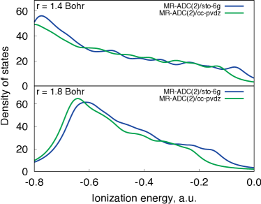
(a)

(b)

Figure 8: (a) Density of states (DOS) for the equally-spaced H30 chain with $r$(H-H) = 1.4 and 1.8 $a_{0}$ computed using MR-ADC(2) with two basis sets and 0.05 $E_{\mathrm{h}}$ broadening. The MR-ADC(2) reference CASSCF wavefunction was computed using the (10e, 10o) active space. (b) Contributions to DOS from core and active orbitals computed using MR-ADC(2) with the STO-6G basis set.

Here, we use MR-ADC to study effect of dynamic correlation and basis set on the density of occupied states in H10 and H30. Figure 7 shows LDOS of H10 for $r$ = 1.4, 1.8, and 3.6 $a_{0}$ computed at the central hydrogen atom using the MR-ADC(0) and MR-ADC(2) methods. We use the full valence (10e, 10o) active space for the CASSCF reference wavefunction and combine MR-ADC with the STO-6G¹⁴⁸ and cc-pVTZ basis sets, plotting LDOS for two broadening parameters: 0.05 $E_{\mathrm{h}}$ (Figure 7) and 0.003 $E_{\mathrm{h}}$ (Supporting Information). For the minimal STO-6G basis, results of MR-ADC(0) and MR-ADC(2) are equivalent to FCI. The computed LDOS are in a very good agreement with LDOS obtained by Ronca et al. employing the dynamical DMRG algorithm for all three geometries.¹⁴⁷ Next, we consider LDOS computed using MR-ADC(0) with the larger cc-pVTZ basis set. Increasing the basis set shifts LDOS to higher ionization energies, relative to LDOS from FCI/STO-6G. For short bond distances ($r$ = 1.4 and 1.8 $a_{0}$), the largest shifts are observed for the lowest-energy peaks corresponding to the ionization potential of the system ($\sim$ 0.03 and 0.05 $E_{\mathrm{h}}$, respectively). For the stretched chain ($r$ = 3.6 $a_{0}$), increasing the basis set compresses LDOS and shifts the position of its maximum by $\sim$ 0.04 $E_{\mathrm{h}}$. Incorporating dynamic correlation effects from MR-ADC(0) to MR-ADC(2) shifts the computed LDOS further to lower energies. For most of the peaks at short bond distances, the computed shifts are $\leq$ 0.02 $E_{\mathrm{h}}$. For $r$ = 3.6 $a_{0}$, including dynamic correlation does not significantly change position of the first band in the spectrum. Overall, our results suggest that increasing the one-electron basis set and incorporating dynamic correlation effects are similarly important and should be both taken into account in accurate computations of LDOS for hydrogen chains.

An attractive feature of MR-ADC is that it is not limited to describing ionization processes only in active orbitals. We demonstrate this by computing total density of occupied states (DOS) for the H30 chain using MR-ADC(2) with the (10e, 10o) active space. Since for this system we do not include all valence orbitals in the active space, we do not consider the stretched $r$ = 3.6 $a_{0}$ geometry. Figure 8a shows MR-ADC(2) DOS computed using the STO-6G and cc-pVDZ basis sets. For both geometries, DOS computed using MR-ADC(2) with the STO-6G basis closely resembles LDOS of the same system from the DMRG study of Ronca et al.¹⁴⁷ Figure 8b plots contributions to MR-ADC(2)/STO-6G DOS from core and active orbitals separately. For the compressed chain ($r$ = 1.4 $a_{0}$), contributions from active orbitals dominate the low-energy part of the spectrum, whereas, for equilibrium geometry ($r$ = 1.8 $a_{0}$), core and active orbitals have similar contributions to DOS already for low ionization energies. Increasing the basis set from STO-6G to cc-pVDZ shifts peaks in DOS to higher energies. As for the H10 chain, the largest shifts are observed for the peak at the first ionization potential.

6 Conclusions

We presented derivation and implementation of second-order multi-reference algebraic diagrammatic construction theory (MR-ADC(2)) for simulating ionization energies and transition properties of strongly correlated systems. In MR-ADC(2), ionization energies and spectral properties are determined from poles and residues of the one-electron Green’s function that is evaluated to second order in multi-reference perturbation theory with respect to a complete active space (CAS) reference wavefunction. In contrast to conventional second-order multi-reference perturbation theories (such as multi-state CASPT2 or NEVPT2), MR-ADC(2) describes ionization in all orbitals (e.g., core and active), does not require using state-averaged wavefunctions to compute higher-energy ionized states, and provides direct access to spectroscopic properties. Although equations of MR-ADC(2) depend on four-particle reduced density matrices, we demonstrated that computation of these large matrices can be completely avoided by constructing efficient intermediates, without introducing any approximations. The resulting MR-ADC(2) implementation has a lower $\mathcal{O}(N_{\mathrm{det}}N^{6}_{\mathrm{act}})$ computational scaling with respect to the number of active orbitals ($N_{\mathrm{act}}$), compared to the $\mathcal{O}(N_{\mathrm{det}}N^{8}_{\mathrm{act}})$ scaling of conventional multi-reference perturbation theories.

We benchmarked accuracy of MR-ADC(2) for predicting ionization energies of eight small molecules, carbon dimer (C2), and hydrogen chains (H10 and H30), against results from full configuration interaction (FCI). For small molecules, MR-ADC(2) shows consistent performance for equilibrium and stretched geometries, with mean absolute errors of $\sim$ 0.5 eV in ionization energies and 0.1 eV in energy separations between ionized states. For C2, MR-ADC(2) predicts energies of the main and singly-excited satellite peaks within 0.4 eV from the FCI reference values, but has a large $\sim$ 0.7 eV error for the doubly-excited satellite transition. The QD-NEVPT2 method shows smaller ($\sim$ 0.1 eV) errors than MR-ADC(2) for all ionized states of C2, providing an improved description of differential dynamic correlation effects, which are important for this system. We expect that these effects will be better described using the higher-order MR-ADC approximations, which will be one of the directions of our future work. Finally, we used MR-ADC(2) to investigate density of occupied states (DOS) in H10 and H30. For H10, our results provide numerical evidence that including dynamic correlation effects beyond those incorporated in a full valence CAS and increasing single-particle basis set have a similar effect on the computed local DOS. Since dynamic correlation is a local phenomenon, we expect that its effect will be similar for longer hydrogen chains as well. For H30, we showed that DOS computed using MR-ADC(2) combined with a small (10e, 10o) active space is in a very good agreement with previously reported results from density matrix renormalization group, incorporating 30 electrons and orbitals in the active space.

Overall, our results suggest that MR-ADC is a promising theoretical approach for computing ionization energies and spectral densities of multi-reference systems and encourage its further development. Future work will be directed towards more efficient implementation of MR-ADC(2) for systems with a large number of electrons and active orbitals, as well as the development of more accurate MR-ADC approximations that will incorporate description of higher-order dynamic correlation effects. We also plan extending our MR-ADC methods to simulations of core-level ionizations in X-ray photoelectron spectroscopy, which has become a widely used tool for experimental investigations of molecules and materials.

This work was supported by start-up funds provided by the Ohio State University. Computations were performed at the Ohio Supercomputer Center under projects PAS1317 and PAS1583.¹⁴⁹ The authors would like to thank Sandeep Sharma for useful suggestions about carrying out SHCI computations.

Comparison of MR-ADC(2) results with exact and approximate second-order amplitudes. Equations of the MR-ADC(2) method for the $\mathbf{M}$, $\mathbf{T}$, and $\mathbf{S}$ matrices. Density of states for H10 with a small broadening parameter.

References

- Olsen et al. 1988 Olsen, J.; Roos, B. O.; Jørgensen, P.; Jensen, H. J. A. Determinant based configuration interaction algorithms for complete and restricted configuration interaction spaces. J. Chem. Phys. 1988, 89, 2185
- Malmqvist et al. 1990 Malmqvist, P. Å.; Rendell, A.; Roos, B. O. The restricted active space self-consistent-field method, implemented with a split graph unitary group approach. J. Phys. Chem. 1990, 94, 5477–5482
- White and Martin 1999 White, S. R.; Martin, R. L. Ab initio quantum chemistry using the density matrix renormalization group. J. Chem. Phys. 1999, 110, 4127
- Legeza et al. 2008 Legeza, Ö.; Noack, R.; Sólyom, J.; Tincani, L. Computational Many-Particle Physics; Springer, 2008; pp 653–664
- Booth et al. 2009 Booth, G. H.; Thom, A. J. W.; Alavi, A. Fermion Monte Carlo without fixed nodes: A game of life, death, and annihilation in Slater determinant space. J. Chem. Phys. 2009, 131, 054106
- Kurashige and Yanai 2009 Kurashige, Y.; Yanai, T. High-performance ab initio density matrix renormalization group method: Applicability to large-scale multireference problems for metal compounds. J. Chem. Phys. 2009, 130, 234114
- Marti and Reiher 2011 Marti, K. H.; Reiher, M. New electron correlation theories for transition metal chemistry. Phys. Chem. Chem. Phys. 2011, 13, 6750–6759
- Chan and Sharma 2011 Chan, G. K.-L.; Sharma, S. The Density Matrix Renormalization Group in Quantum Chemistry. Annu. Rev. Phys. Chem. 2011, 62, 465–481
- Gunst et al. 2014 Gunst, K.; Wouters, S.; De Baerdemacker, S.; Van Neck, D. Block product density matrix embedding theory for strongly correlated spin systems. Eur. Phys. J. D 2014, 68, 272
- Zhang and Evangelista 2016 Zhang, T.; Evangelista, F. A. A Deterministic Projector Configuration Interaction Approach for the Ground State of Quantum Many-Body Systems. J. Chem. Theory Comput. 2016, 12, 4326–4337
- Schriber and Evangelista 2017 Schriber, J. B.; Evangelista, F. A. Adaptive Configuration Interaction for Computing Challenging Electronic Excited States with Tunable Accuracy. J. Chem. Theory Comput. 2017, 13, 5354–5366
- Holmes et al. 2016 Holmes, A. A.; Tubman, N. M.; Umrigar, C. J. Heat-Bath Configuration Interaction: An Efficient Selected Configuration Interaction Algorithm Inspired by Heat-Bath Sampling. J. Chem. Theory Comput. 2016, 12, 3674–3680
- Sharma et al. 2017 Sharma, S.; Holmes, A. A.; Jeanmairet, G.; Alavi, A.; Umrigar, C. J. Semistochastic Heat-Bath Configuration Interaction Method: Selected Configuration Interaction with Semistochastic Perturbation Theory. J. Chem. Theory Comput. 2017, 13, 1595–1604
- Holmes et al. 2017 Holmes, A. A.; Umrigar, C. J.; Sharma, S. Excited states using semistochastic heat-bath configuration interaction. J. Chem. Phys. 2017, 147, 164111
- Werner and Meyer 1980 Werner, H.-J.; Meyer, W. A quadratically convergent multiconfiguration–self-consistent field method with simultaneous optimization of orbitals and CI coefficients. J. Chem. Phys. 1980, 73, 2342–2356
- Werner 1981 Werner, H.-J. A quadratically convergent MCSCF method for the simultaneous optimization of several states. J. Chem. Phys. 1981, 74, 5794–5801
- Knowles and Werner 1985 Knowles, P. J.; Werner, H.-J. An efficient second-order MC SCF method for long configuration expansions. Chem. Phys. Lett. 1985, 115, 259–267
- Wolinski et al. 1987 Wolinski, K.; Sellers, H. L.; Pulay, P. Consistent generalization of the Møller-Plesset partitioning to open-shell and multiconfigurational SCF reference states in many-body perturbation theory. Chem. Phys. Lett. 1987, 140, 225–231
- Hirao 1992 Hirao, K. Multireference Møller—Plesset method. Chem. Phys. Lett. 1992, 190, 374–380
- Werner 1996 Werner, H.-J. Third-order multireference perturbation theory. The CASPT3 method. Mol. Phys. 1996, 89, 645–661
- Finley et al. 1998 Finley, J. P.; Malmqvist, P. Å.; Roos, B. O.; Serrano-Andrés, L. The multi-state CASPT2 method. Chem. Phys. Lett. 1998, 288, 299–306
- Andersson et al. 1990 Andersson, K.; Malmqvist, P. Å.; Roos, B. O.; Sadlej, A. J.; Wolinski, K. Second-order perturbation theory with a CASSCF reference function. J. Phys. Chem. 1990, 94, 5483–5488
- Andersson et al. 1992 Andersson, K.; Malmqvist, P. Å.; Roos, B. O. Second-order perturbation theory with a complete active space self-consistent field reference function. J. Chem. Phys. 1992, 96, 1218–1226
- Angeli et al. 2001 Angeli, C.; Cimiraglia, R.; Evangelisti, S.; Leininger, T.; Malrieu, J.-P. P. Introduction of n-electron valence states for multireference perturbation theory. J. Chem. Phys. 2001, 114, 10252–10264
- Angeli et al. 2001 Angeli, C.; Cimiraglia, R.; Malrieu, J.-P. P. N-electron valence state perturbation theory: a fast implementation of the strongly contracted variant. Chem. Phys. Lett. 2001, 350, 297–305
- Angeli et al. 2004 Angeli, C.; Borini, S.; Cestari, M.; Cimiraglia, R. A quasidegenerate formulation of the second order n-electron valence state perturbation theory approach. J. Chem. Phys. 2004, 121, 4043–4049
- Li and Evangelista 2015 Li, C.; Evangelista, F. A. Multireference Driven Similarity Renormalization Group: A Second-Order Perturbative Analysis. J. Chem. Theory Comput. 2015, 11, 2097–2108
- Buenker and Peyerimhoff 1974 Buenker, R. J.; Peyerimhoff, S. D. Individualized configuration selection in CI calculations with subsequent energy extrapolation. Theor. Chem. Acc. 1974, 35, 33–58
- Siegbahn 1980 Siegbahn, P. E. M. Generalizations of the direct CI method based on the graphical unitary group approach. II. Single and double replacements from any set of reference configurations. J. Chem. Phys. 1980, 72, 1647
- Werner and Knowles 1988 Werner, H.-J.; Knowles, P. J. An efficient internally contracted multiconfiguration–reference configuration interaction method. J. Chem. Phys. 1988, 89, 5803–5814
- Saitow et al. 2013 Saitow, M.; Kurashige, Y.; Yanai, T. Multireference configuration interaction theory using cumulant reconstruction with internal contraction of density matrix renormalization group wave function. J. Chem. Phys. 2013, 139, 044118
- Saitow et al. 2015 Saitow, M.; Kurashige, Y.; Yanai, T. Fully Internally Contracted Multireference Configuration Interaction Theory Using Density Matrix Renormalization Group: A Reduced-Scaling Implementation Derived by Computer-Aided Tensor Factorization. J. Chem. Theory Comput. 2015, 11, 5120–5131
- Mukherjee et al. 1977 Mukherjee, D.; Moitra, R. K.; Mukhopadhyay, A. Applications of a non-perturbative many-body formalism to general open-shell atomic and molecular problems: calculation of the ground and the lowest -* singlet and triplet energies and the first ionization potential of trans-butadiene. Mol. Phys. 1977, 33, 955–969
- Lindgren 1978 Lindgren, I. A coupled-cluster approach to the many-body perturbation theory for open-shell systems. Int. J. Quantum Chem. 1978, 14, 33–58
- Jeziorski and Monkhorst 1981 Jeziorski, B.; Monkhorst, H. J. Coupled-cluster method for multideterminantal reference states. Phys. Rev. A 1981, 24, 1668–1681
- Mahapatra et al. 1999 Mahapatra, U. S.; Datta, B.; Mukherjee, D. A size-consistent state-specific multireference coupled cluster theory: Formal developments and molecular applications. J. Chem. Phys. 1999, 110, 6171
- Evangelista et al. 2007 Evangelista, F. A.; Allen, W. D.; Schaefer, H. F. Coupling term derivation and general implementation of state-specific multireference coupled cluster theories. J. Chem. Phys. 2007, 127, 024102
- Datta et al. 2011 Datta, D.; Kong, L.; Nooijen, M. A state-specific partially internally contracted multireference coupled cluster approach. J. Chem. Phys. 2011, 134, 214116
- Evangelista and Gauss 2011 Evangelista, F. A.; Gauss, J. An orbital-invariant internally contracted multireference coupled cluster approach. J. Chem. Phys. 2011, 134, 114102
- Köhn et al. 2013 Köhn, A.; Hanauer, M.; Mück, L. A.; Jagau, T.-C.; Gauss, J. State-specific multireference coupled-cluster theory. WIREs Comput. Mol. Sci. 2013, 3, 176–197
- Datta and Nooijen 2012 Datta, D.; Nooijen, M. Multireference equation-of-motion coupled cluster theory. J. Chem. Phys. 2012, 137, 204107
- Nooijen et al. 2014 Nooijen, M.; Demel, O.; Datta, D.; Kong, L.; Shamasundar, K. R.; Lotrich, V.; Huntington, L. M.; Neese, F. Communication: Multireference equation of motion coupled cluster: A transform and diagonalize approach to electronic structure. J. Chem. Phys. 2014, 140, 081102
- Huntington and Nooijen 2015 Huntington, L. M. J.; Nooijen, M. Application of multireference equation of motion coupled-cluster theory to transition metal complexes and an orbital selection scheme for the efficient calculation of excitation energies. J. Chem. Phys. 2015, 142, 194111
- Kirtman 1998 Kirtman, B. Simultaneous calculation of several interacting electronic states by generalized Van Vleck perturbation theory. J. Chem. Phys. 1998, 75, 798–808
- Hoffmann and Simons 1988 Hoffmann, M. R. R.; Simons, J. A unitary multiconfigurational coupled-cluster method: Theory and applications. J. Chem. Phys. 1988, 88, 993
- Yanai and Chan 2006 Yanai, T.; Chan, G. K.-L. Canonical transformation theory for multireference problems. J. Chem. Phys. 2006, 124, 194106
- Yanai and Chan 2007 Yanai, T.; Chan, G. K.-L. Canonical transformation theory from extended normal ordering. J. Chem. Phys. 2007, 127, 104107
- Chen and Hoffmann 2012 Chen, Z.; Hoffmann, M. R. R. Orbitally invariant internally contracted multireference unitary coupled cluster theory and its perturbative approximation: Theory and test calculations of second order approximation. J. Chem. Phys. 2012, 137, 014108
- Li and Evangelista 2016 Li, C.; Evangelista, F. A. Towards numerically robust multireference theories: The driven similarity renormalization group truncated to one- and two-body operators. J. Chem. Phys. 2016, 144, 164114
- Evangelista 2018 Evangelista, F. A. Perspective: Multireference coupled cluster theories of dynamical electron correlation. J. Chem. Phys. 2018, 149, 030901
- Kurashige and Yanai 2011 Kurashige, Y.; Yanai, T. Second-order perturbation theory with a density matrix renormalization group self-consistent field reference function: Theory and application to the study of chromium dimer. J. Chem. Phys. 2011, 135, 094104
- Kurashige et al. 2014 Kurashige, Y.; Chalupský, J.; Lan, T. N.; Yanai, T. Complete active space second-order perturbation theory with cumulant approximation for extended active-space wavefunction from density matrix renormalization group. J. Chem. Phys. 2014, 141, 174111
- Guo et al. 2016 Guo, S.; Watson, M. A.; Hu, W.; Sun, Q.; Chan, G. K.-L. N-Electron Valence State Perturbation Theory Based on a Density Matrix Renormalization Group Reference Function, with Applications to the Chromium Dimer and a Trimer Model of Poly(p-Phenylenevinylene). J. Chem. Theory Comput. 2016, 12, 1583–1591
- Sharma et al. 2017 Sharma, S.; Knizia, G.; Guo, S.; Alavi, A. Combining Internally Contracted States and Matrix Product States To Perform Multireference Perturbation Theory. J. Chem. Theory Comput. 2017, 13, 488–498
- Yanai et al. 2017 Yanai, T.; Saitow, M.; Xiong, X.-G.; Chalupský, J.; Kurashige, Y.; Guo, S.; Sharma, S. Multistate Complete-Active-Space Second-Order Perturbation Theory Based on Density Matrix Renormalization Group Reference States. J. Chem. Theory Comput. 2017, 13, 4829–4840
- Freitag et al. 2017 Freitag, L.; Knecht, S.; Angeli, C.; Reiher, M. Multireference Perturbation Theory with Cholesky Decomposition for the Density Matrix Renormalization Group. J. Chem. Theory Comput. 2017, 13, 451
- Sokolov et al. 2017 Sokolov, A. Y.; Guo, S.; Ronca, E.; Chan, G. K.-L. Time-dependent N-electron valence perturbation theory with matrix product state reference wavefunctions for large active spaces and basis sets: Applications to the chromium dimer and all-trans polyenes. J. Chem. Phys. 2017, 146, 244102
- Schriber et al. 2018 Schriber, J. B.; Hannon, K. P.; Li, C.; Evangelista, F. A. A Combined Selected Configuration Interaction and Many-Body Treatment of Static and Dynamical Correlation in Oligoacenes. J. Chem. Theory Comput. 2018, 14, 6295–6305
- MacLeod and Shiozaki 2015 MacLeod, M. K.; Shiozaki, T. Communication: Automatic code generation enables nuclear gradient computations for fully internally contracted multireference theory. J. Chem. Phys. 2015, 142, 051103
- Sokolov 2018 Sokolov, A. Y. Multi-reference algebraic diagrammatic construction theory for excited states: General formulation and first-order implementation. J. Chem. Phys. 2018, 149, 204113
- Schirmer 1982 Schirmer, J. Beyond the random-phase approximation: A new approximation scheme for the polarization propagator. Phys. Rev. A 1982, 26, 2395–2416
- Banerjee et al. 1978 Banerjee, A.; Shepard, R.; Simons, J. One-particle Green’s function with multiconfiguration reference states. Int. J. Quantum Chem. 1978, 14, 389–404
- Yeager and Jørgensen 1979 Yeager, D. L.; Jørgensen, P. A multiconfigurational time-dependent Hartree-Fock approach. Chem. Phys. Lett. 1979, 65, 77–80
- Dalgaard 1980 Dalgaard, E. Time-dependent multiconfigurational Hartree–Fock theory. J. Chem. Phys. 1980, 72, 816–823
- Yeager et al. 1984 Yeager, D. L.; Olsen, J.; Jørgensen, P. Generalizations of the multiconfigurational time-dependent Hartree-Fock approach. Faraday Symp. Chem. Soc. 1984, 19, 85–95
- Graham and Yeager 1991 Graham, R. L.; Yeager, D. L. The multiconfigurational particle–particle propagator method for directly determining vertical double ionization potentials and double electron affinities. J. Chem. Phys. 1991, 94, 2884–2893
- Yeager 1992 Yeager, D. L. Applied Many-Body Methods in Spectroscopy and Electronic Structure; Springer, Boston, MA: Boston, MA, 1992; pp 133–161
- Nichols et al. 1998 Nichols, J. A.; Yeager, D. L.; Jørgensen, P. Multiconfigurational electron propagator (MCEP) ionization potentials for general open shell systems. J. Chem. Phys. 1998, 80, 293–314
- Khrustov and Kostychev 2002 Khrustov, V. F.; Kostychev, D. E. Multiconfigurational Green’s function approach with quasidegenerate perturbation theory. Int. J. Quantum Chem. 2002, 88, 507–518
- Helmich-Paris 2019 Helmich-Paris, B. CASSCF linear response calculations for large open-shell molecules. J. Chem. Phys. 2019, 150, 174121
- Samanta et al. 2014 Samanta, P. K.; Mukherjee, D.; Hanauer, M.; Köhn, A. Excited states with internally contracted multireference coupled-cluster linear response theory. J. Chem. Phys. 2014, 140, 134108
- Mukherjee and Kutzelnigg 1989 Mukherjee, D.; Kutzelnigg, W. Many-Body Methods in Quantum Chemistry; Springer, Berlin, Heidelberg: Berlin, Heidelberg, 1989; pp 257–274
- Fetter and Walecka 2003 Fetter, A. L.; Walecka, J. D. Quantum theory of many-particle systems; Dover Publications, 2003
- Dickhoff and Van Neck 2005 Dickhoff, W. H.; Van Neck, D. Many-body theory exposed!: propagator description of quantum mechanics in many-body systems; World Scientific Publishing Co., 2005
- Goscinski and Weiner 1980 Goscinski, O.; Weiner, B. The Role of Algebraic Formulations of Approximate Green’s Functions for Systems With a Finite Number of Electrons. Phys. Scr. 1980, 21, 385–393
- Weiner and Goscinski 1980 Weiner, B.; Goscinski, O. Self-consistent approximation to the polarization propagator. Int. J. Quantum Chem. 1980, 18, 1109–1131
- Prasad et al. 1985 Prasad, M. D.; Pal, S.; Mukherjee, D. Some aspects of self-consistent propagator theories. Phys. Rev. A 1985, 31, 1287–1298
- Datta et al. 1993 Datta, B.; Mukhopadhyay, D.; Mukherjee, D. Consistent propagator theory based on the extended coupled-cluster parametrization of the ground state. Phys. Rev. A 1993, 47, 3632–3648
- Löwdin 1970 Löwdin, P. O. Some properties of inner projections. Int. J. Quantum Chem. 1970, 5, 231–237
- Nielsen et al. 1980 Nielsen, E. S.; Jørgensen, P.; Oddershede, J. Transition moments and dynamic polarizabilities in a second order polarization propagator approach. J. Chem. Phys. 1980, 73, 6238–6246
- Sangfelt et al. 1984 Sangfelt, E.; Kurtz, H. A.; Elander, N.; Goscinski, O. Excited states via the AGP polarization propagator. I. Application to Li2. J. Chem. Phys. 1984, 81, 3976–3986
- Bak et al. 2000 Bak, K. L.; Koch, H.; Oddershede, J.; Christiansen, O.; Sauer, S. P. A. Atomic integral driven second order polarization propagator calculations of the excitation spectra of naphthalene and anthracene. J. Chem. Phys. 2000, 112, 4173–4185
- Nooijen and Snijders 1992 Nooijen, M.; Snijders, J. G. Coupled cluster approach to the single-particle Green’s function. Int. J. Quantum Chem. 1992, 44, 55–83
- Nooijen and Snijders 1993 Nooijen, M.; Snijders, J. G. Coupled cluster Green’s function method: Working equations and applications. Int. J. Quantum Chem. 1993, 48, 15–48
- Nooijen and Snijders 1995 Nooijen, M.; Snijders, J. G. Second order many-body perturbation approximations to the coupled cluster Green’s function. J. Chem. Phys. 1995, 102, 1681–1688
- Moszynski et al. 2005 Moszynski, R.; Żuchowski, P. S.; Jeziorski, B. Time-Independent Coupled-Cluster Theory of the Polarization Propagator. Collect. Czech. Chem. Commun. 2005, 70, 1109–1132
- Korona 2010 Korona, T. XCC2—a new coupled cluster model for the second-order polarization propagator. Phys. Chem. Chem. Phys. 2010, 12, 14977–14984
- Kowalski et al. 2014 Kowalski, K.; Bhaskaran-Nair, K.; Shelton, W. A. Coupled-cluster representation of Green function employing modified spectral resolutions of similarity transformed Hamiltonians. J. Chem. Phys. 2014, 141, 094102
- Schirmer 1991 Schirmer, J. Closed-form intermediate representations of many-body propagators and resolvent matrices. Phys. Rev. A 1991, 43, 4647
- Mertins and Schirmer 1996 Mertins, F.; Schirmer, J. Algebraic propagator approaches and intermediate-state representations. I. The biorthogonal and unitary coupled-cluster methods. Phys. Rev. A 1996, 53, 2140–2152
- Schirmer and Trofimov 2004 Schirmer, J.; Trofimov, A. B. Intermediate state representation approach to physical properties of electronically excited molecules. J. Chem. Phys. 2004, 120, 11449–11464
- Schirmer et al. 1983 Schirmer, J.; Cederbaum, L. S.; Walter, O. New approach to the one-particle Green’s function for finite Fermi systems. Phys. Rev. A 1983, 28, 1237–1259
- Schirmer et al. 1998 Schirmer, J.; Trofimov, A. B.; Stelter, G. A non-Dyson third-order approximation scheme for the electron propagator. J. Chem. Phys. 1998, 109, 4734
- Trofimov and Schirmer 2005 Trofimov, A. B.; Schirmer, J. Molecular ionization energies and ground- and ionic-state properties using a non-Dyson electron propagator approach. J. Chem. Phys. 2005, 123, 144115
- Dempwolff et al. 2019 Dempwolff, A. L.; Schneider, M.; Hodecker, M.; Dreuw, A. Efficient implementation of the non-Dyson third-order algebraic diagrammatic construction approximation for the electron propagator for closed- and open-shell molecules. J. Chem. Phys. 2019, 150, 064108
- Liu et al. 2018 Liu, J.; Asthana, A.; Cheng, L.; Mukherjee, D. Unitary coupled-cluster based self-consistent polarization propagator theory: A third-order formulation and pilot applications. J. Chem. Phys. 2018, 148, 244110
- Hedin 1965 Hedin, L. New method for calculating the one-particle Green’s function with application to the electron-gas problem. Phys. Rev. A 1965, 139, 796–823
- Faleev et al. 2004 Faleev, S. V.; van Schilfgaarde, M.; Kotani, T. All-Electron Self-Consistent GW Approximation: Application to Si, MnO, and NiO. Phys. Rev. Lett. 2004, 93, 126406
- van Schilfgaarde et al. 2006 van Schilfgaarde, M.; Kotani, T.; Faleev, S. Quasiparticle Self-Consistent GW Theory. Phys. Rev. Lett. 2006, 96, 226402
- Cederbaum 1975 Cederbaum, L. S. One-body Green’s function for atoms and molecules. J. Phys. B: At. Mol. Phys. 1975, 8, 290–303
- Von Niessen et al. 1984 Von Niessen, W.; Schirmer, J.; Cederbaum, L. S. Computational methods for the one-particle Green’s function. Computer Physics Reports 1984, 1, 57–125
- Ortiz 2012 Ortiz, J. V. Electron propagator theory: an approach to prediction and interpretation in quantum chemistry. WIREs Comput. Mol. Sci. 2012, 3, 123–142
- Georges et al. 1996 Georges, A.; Kotliar, G.; Krauth, W.; Rozenberg, M. J. Dynamical mean-field theory of strongly correlated fermion systems and the limit of infinite dimensions. Rev. Mod. Phys. 1996, 68, 13–125
- Kotliar et al. 2006 Kotliar, G.; Savrasov, S. Y.; Haule, K.; Oudovenko, V. S.; Parcollet, O.; Marianetti, C. A. Electronic structure calculations with dynamical mean-field theory. Rev. Mod. Phys. 2006, 78, 865–951
- Phillips and Zgid 2014 Phillips, J. J.; Zgid, D. Communication: The description of strong correlation within self-consistent Green’s function second-order perturbation theory. J. Chem. Phys. 2014, 140, 241101
- Lan et al. 2015 Lan, T. N.; Kananenka, A. A.; Zgid, D. Communication: Towards ab initio self-energy embedding theory in quantum chemistry. J. Chem. Phys. 2015, 143, 241102
- Dyall 1995 Dyall, K. G. The choice of a zeroth-order Hamiltonian for second-order perturbation theory with a complete active space self-consistent-field reference function. J. Chem. Phys. 1995, 102, 4909–4918
- Aoto et al. 2019 Aoto, Y. A.; Bargholz, A.; Kats, D.; Werner, H.-J.; Köhn, A. Perturbation Expansion of Internally Contracted Coupled-Cluster Theory up to Third Order. J. Chem. Theory Comput. 2019, 15, 2291–2305
- Freed and Yeager 1977 Freed, K. F.; Yeager, D. L. A wavefunction approach to equations of motion—Green’s function methods. Chem. Phys. 1977, 22, 401–414
- Löwdin 1985 Löwdin, P. O. Some Aspects on the Hamiltonian and Liouvillian Formalism, the Special Propagator Methods, and the Equation of Motion Approach. Adv. Quant. Chem. 1985, 17, 285–334
- Kutzelnigg and Mukherjee 1989 Kutzelnigg, W.; Mukherjee, D. Time-independent theory of one-particle Green’s functions. J. Chem. Phys. 1989, 90, 5578–5594
- Bofill and Pulay 1998 Bofill, J. M.; Pulay, P. The unrestricted natural orbital–complete active space (UNO–CAS) method: An inexpensive alternative to the complete active space–self-consistent-field (CAS–SCF) method. J. Chem. Phys. 1998, 90, 3637–3646
- Neuscamman et al. 2009 Neuscamman, E.; Yanai, T.; Chan, G. K.-L. Quadratic canonical transformation theory and higher order density matrices. J. Chem. Phys. 2009, 130, 124102
- Hanauer and Köhn 2011 Hanauer, M.; Köhn, A. Pilot applications of internally contracted multireference coupled cluster theory, and how to choose the cluster operator properly. J. Chem. Phys. 2011, 134, 204111
- Hanauer and Köhn 2012 Hanauer, M.; Köhn, A. Communication: Restoring full size extensivity in internally contracted multireference coupled cluster theory. J. Chem. Phys. 2012, 137, 131103
- Sokolov and Chan 2016 Sokolov, A. Y.; Chan, G. K.-L. A time-dependent formulation of multi-reference perturbation theory. J. Chem. Phys. 2016, 144, 064102
- Wouters et al. 2016 Wouters, S.; Van Speybroeck, V.; Van Neck, D. DMRG-CASPT2 study of the longitudinal static second hyperpolarizability of all-trans polyenes. J. Chem. Phys. 2016, 145, 054120
- Davidson 1975 Davidson, E. R. The iterative calculation of a few of the lowest eigenvalues and corresponding eigenvectors of large real-symmetric matrices. J. Comput. Phys. 1975, 17, 87
- Liu 1978 Liu, B. The Simultaneous Expansion Method for the Iterative Solution of Several of the Lowest-Lying Eigenvalues and Corresponding Eigenvectors of Large Real-Symmetric Matrices; 1978; pp 49–53
- Sun et al. 2018 Sun, Q.; Berkelbach, T. C.; Blunt, N. S.; Booth, G. H.; Guo, S.; Li, Z.; Liu, J.; McClain, J. D.; Sayfutyarova, E. R.; Sharma, S.; Wouters, S.; Chan, G. K.-L. PySCF: the Python-based simulations of chemistry framework. WIREs Comput. Mol. Sci. 2018, 8, e1340
- Press et al. 1986 Press, W. H.; Teukolsky, S. A.; Vetterling, W. T.; Flannery, B. P. Numerical Recipes: The Art of Scientific Computing; Cambridge University Press: New York, 1986
- Kendall et al. 1992 Kendall, R. A.; Dunning Jr, T. H.; Harrison, R. J. Electron affinities of the first-row atoms revisited. Systematic basis sets and wave functions. 1992, 96, 6796–6806
- Sinha et al. 1989 Sinha, D.; Mukhopadhyay, S. K.; Chaudhuri, R.; Mukherjee, D. The eigenvalue-independent partitioning technique in Fock space: An alternative route to open-shell coupled-cluster theory for incomplete model spaces. Chem. Phys. Lett. 1989, 154, 544–549
- Mukhopadhyay et al. 1991 Mukhopadhyay, D.; Mukhopadhyay, S.; Chaudhuri, R.; Mukherjee, D. Aspects of separability in the coupled cluster based direct methods for energy differences. Theoret. Chim. Acta 1991, 80, 441–467
- Shao et al. 2015 Shao, Y.; Gan, Z.; Epifanovsky, E.; Gilbert, A. T.; Wormit, M.; Kussmann, J.; Lange, A. W.; Behn, A.; Deng, J.; Feng, X.; Ghosh, D.; Goldey, M.; Horn, P. R.; Jacobson, L. D.; Kaliman, I.; Khaliullin, R. Z.; Kuś, T.; Landau, A.; Liu, J.; Proynov, E. I.; Rhee, Y. M.; Richard, R. M.; Rohrdanz, M. A.; Steele, R. P.; Sundstrom, E. J.; III, H. L. W.; Zimmerman, P. M.; Zuev, D.; Albrecht, B.; Alguire, E.; Austin, B.; Beran, G. J. O.; Bernard, Y. A.; Berquist, E.; Brandhorst, K.; Bravaya, K. B.; Brown, S. T.; Casanova, D.; Chang, C.-M.; Chen, Y.; Chien, S. H.; Closser, K. D.; Crittenden, D. L.; Diedenhofen, M.; Jr., R. A. D.; Do, H.; Dutoi, A. D.; Edgar, R. G.; Fatehi, S.; Fusti-Molnar, L.; Ghysels, A.; Golubeva-Zadorozhnaya, A.; Gomes, J.; Hanson-Heine, M. W.; Harbach, P. H.; Hauser, A. W.; Hohenstein, E. G.; Holden, Z. C.; Jagau, T.-C.; Ji, H.; Kaduk, B.; Khistyaev, K.; Kim, J.; Kim, J.; King, R. A.; Klunzinger, P.; Kosenkov, D.; Kowalczyk, T.; Krauter, C. M.; Lao, K. U.; Laurent, A. D.; Lawler, K. V.; Levchenko, S. V.; Lin, C. Y.; Liu, F.; Livshits, E.; Lochan, R. C.; Luenser, A.; Manohar, P.; Manzer, S. F.; Mao, S.-P.; Mardirossian, N.; Marenich, A. V.; Maurer, S. A.; Mayhall, N. J.; Neuscamman, E.; Oana, C. M.; Olivares-Amaya, R.; O’Neill, D. P.; Parkhill, J. A.; Perrine, T. M.; Peverati, R.; Prociuk, A.; Rehn, D. R.; Rosta, E.; Russ, N. J.; Sharada, S. M.; Sharma, S.; Small, D. W.; Sodt, A.; Stein, T.; Stück, D.; Su, Y.-C.; Thom, A. J.; Tsuchimochi, T.; Vanovschi, V.; Vogt, L.; Vydrov, O.; Wang, T.; Watson, M. A.; Wenzel, J.; White, A.; Williams, C. F.; Yang, J.; Yeganeh, S.; Yost, S. R.; You, Z.-Q.; Zhang, I. Y.; Zhang, X.; Zhao, Y.; Brooks, B. R.; Chan, G. K.; Chipman, D. M.; Cramer, C. J.; III, W. A. G.; Gordon, M. S.; Hehre, W. J.; Klamt, A.; III, H. F. S.; Schmidt, M. W.; Sherrill, C. D.; Truhlar, D. G.; Warshel, A.; Xu, X.; Aspuru-Guzik, A.; Baer, R.; Bell, A. T.; Besley, N. A.; Chai, J.-D.; Dreuw, A.; Dunietz, B. D.; Furlani, T. R.; Gwaltney, S. R.; Hsu, C.-P.; Jung, Y.; Kong, J.; Lambrecht, D. S.; Liang, W.; Ochsenfeld, C.; Rassolov, V. A.; Slipchenko, L. V.; Subotnik, J. E.; Voorhis, T. V.; Herbert, J. M.; Krylov, A. I.; Gill, P. M.; Head-Gordon, M. Advances in molecular quantum chemistry contained in the Q-Chem 4 program package. Mol. Phys. 2015, 113, 184–215
- Neese 2017 Neese, F. Software update: the ORCA program system, version 4.0. WIREs Comput. Mol. Sci. 2017, 8, e1327
- Gozem et al. 2015 Gozem, S.; Gunina, A. O.; Ichino, T.; Osborn, D. L.; Stanton, J. F.; Krylov, A. I. Photoelectron Wave Function in Photoionization: Plane Wave or Coulomb Wave? 2015, 6, 4532–4540
- Branton et al. 1970 Branton, G. R.; Frost, D. C.; Makita, T.; McDowell, C. A.; Stenhouse, I. A. Photoelectron Spectra of Ethylene and Ethylene-d4. J. Chem. Phys. 1970, 52, 802–806
- Roos 1987 Roos, B. O. The Complete Active Space Self-Consistent Field Method and its Applications in Electronic Structure Calculations. Adv. Chem. Phys. 1987, 69, 399–445
- Bauschlicher Jr and Langhoff 1987 Bauschlicher Jr, C. W.; Langhoff, S. R. Ab initio calculations on C2, Si2, and SiC. J. Chem. Phys. 1987, 87, 2919
- Watts and Bartlett 1992 Watts, J. D.; Bartlett, R. J. Coupled-cluster calculations on the C2 molecule and the C and C molecular ions. J. Chem. Phys. 1992, 96, 6073
- Abrams and Sherrill 2004 Abrams, M. L.; Sherrill, C. D. Full configuration interaction potential energy curves for the X1, B1g, and B states of C2: A challenge for approximate methods. J. Chem. Phys. 2004, 121, 9211
- Wouters et al. 2014 Wouters, S.; Poelmans, W.; Ayers, P. W.; Van Neck, D. CheMPS2: A free open-source spin-adapted implementation of the density matrix renormalization group for ab initio quantum chemistry. Comput. Phys. Commun. 2014, 185, 1501–1514
- Rosmus et al. 1986 Rosmus, P.; Werner, H.-J.; Reinsch, E. A.; Larsson, M. Multireference CI calculations of radiative transition probabilities between low lying quartet states of the C ion. J. Electron. Spectrosc. Relat. Phenom. 1986, 41, 289–296
- Kraemer and Roos 1987 Kraemer, W. P.; Roos, B. O. A CAS SCF CI study of the 1 and 3u states of the C2 molecule and the 4 and 2u states of the C ion. Chem. Phys. 1987, 118, 345–355
- Watts and Bartlett 1998 Watts, J. D.; Bartlett, R. J. Coupled-cluster calculations on the C2 molecule and the C and C molecular ions. J. Chem. Phys. 1998, 96, 6073–6084
- Petrongolo et al. 1998 Petrongolo, C.; Bruna, P. J.; Peyerimhoff, S. D.; Buenker, R. J. Theoretical prediction of the potential curves for the lowest-lying states of the C molecular ion. J. Chem. Phys. 1998, 74, 4594–4602
- Ballance and McLaughlin 2001 Ballance, C. P.; McLaughlin, B. M. Valence configuration interaction study of the C cation. J. Phys. B: At. Mol. Opt. Phys. 2001, 34, 1201–1212
- Shi et al. 2013 Shi, D.; Niu, X.; Sun, J.; Zhu, Z. Potential Energy Curves, Spectroscopic Parameters, and Spin–Orbit Coupling: A Theoretical Study on 24 -S and 54 States of C Cation. J. Phys. Chem. A 2013, 117, 2020–2034
- Sinitskiy et al. 2010 Sinitskiy, A. V.; Greenman, L.; Mazziotti, D. A. Strong correlation in hydrogen chains and lattices using the variational two-electron reduced density matrix method. J. Chem. Phys. 2010, 133, 014104
- Stella et al. 2011 Stella, L.; Attaccalite, C.; Sorella, S.; Rubio, A. Strong electronic correlation in the hydrogen chain: A variational Monte Carlo study. Phys. Rev. B 2011, 84, 245117
- Lin et al. 2011 Lin, N.; Marianetti, C. A.; Millis, A. J.; Reichman, D. R. Dynamical Mean-Field Theory for Quantum Chemistry. Phys. Rev. Lett. 2011, 106, 096402
- Tsuchimochi and Scuseria 2009 Tsuchimochi, T.; Scuseria, G. E. Strong correlations via constrained-pairing mean-field theory. J. Chem. Phys. 2009, 131, 121102
- Rusakov and Zgid 2016 Rusakov, A. A.; Zgid, D. Self-consistent second-order Green’s function perturbation theory for periodic systems. J. Chem. Phys. 2016, 144, 054106
- Motta et al. 2017 Motta, M.; Ceperley, D. M.; Chan, G. K.-L.; Gomez, J. A.; Gull, E.; Guo, S.; Jiménez-Hoyos, C. A.; Lan, T. N.; Li, J.; Ma, F.; Millis, A. J.; Prokof’ev, N. V.; Ray, U.; Scuseria, G. E.; Sorella, S.; Stoudenmire, E. M.; Sun, Q.; Tupitsyn, I. S.; White, S. R.; Zgid, D.; Zhang, S. Towards the Solution of the Many-Electron Problem in Real Materials: Equation of State of the Hydrogen Chain with State-of-the-Art Many-Body Methods. Phys. Rev. X 2017, 7, 031059
- Rusakov et al. 2019 Rusakov, A. A.; Iskakov, S.; Tran, L. N.; Zgid, D. Self-Energy Embedding Theory (SEET) for Periodic Systems. J. Chem. Theory Comput. 2019, 15, 229–240
- Ronca et al. 2017 Ronca, E.; Li, Z.; Jiménez-Hoyos, C. A.; Chan, G. K.-L. Time-Step Targeting Time-Dependent and Dynamical Density Matrix Renormalization Group Algorithms with ab Initio Hamiltonians. J. Chem. Theory Comput. 2017, 13, 5560–5571
- Hehre et al. 1969 Hehre, W. J.; Stewart, R. F.; Pople, J. A. Self-Consistent Molecular-Orbital Methods. I. Use of Gaussian Expansions of Slater-Type Atomic Orbitals. J. Chem. Phys. 1969, 51, 2657–2664
- Ohi 1987 Ohio Supercomputer Center. 1987; http://osc.edu/ark:/19495/f5s1ph73