Counting and Segmenting Sorghum Heads

Abstract

Phenotyping is the process of measuring an organism’s observable traits. Manual phenotyping of crops is a labor-intensive, time-consuming, costly, and error prone process. Accurate, automated, high-throughput phenotyping can relieve a huge burden in the crop breeding pipeline. In this paper, we propose a scalable, high-throughput approach to automatically count and segment panicles (heads), a key phenotype, from aerial sorghum crop imagery. Our counting approach uses the image density map obtained from dot or region annotation as the target with a novel deep convolutional neural network architecture. We also propose a novel instance segmentation algorithm using the estimated density map, to identify the individual panicles in the presence of occlusion. With real Sorghum aerial images, we obtain a mean absolute error (MAE) of 1.06 for counting which is better than using well-known crowd counting approaches such as CCNN, MCNN and CSRNet models. The instance segmentation model also produces respectable results which will be ultimately useful in reducing the manual annotation workload for future data.

1 Introduction

Genotyping and phenotyping constitute two key components of plant breeding. Genotyping involves the understanding of the genetic constitution of plants, whereas phenotyping involves the measurement of their observable traits. While genotyping has become more accurate and affordable, phenotyping has become the bottleneck in accelerated breeding programs [17]. This is because manual phenotyping methods are labor-intensive, inaccurate, and expensive.

In this paper, we develop methods to automatically count and segment panicles for Sorghum crops using a novel two-stage convolutional neural network (CNN) architecture that uses the panicle density map as target. Panicles are the heads of the plant that carry the grain. They are one of the most important phenotypes in crop breeding, since they correlate highly to the grain yield [35], which is directly useful for food and feed. Panicles also constitute a substantial fraction of the biomass, which can be used for sustainable bio-fuel production. The work presented here is incorporated in a high-throughput phenotyping pipeline being developed as a part of the Department of Energy’s “Transportation Energy Resources from Renewable Agriculture Phenotyping” (TERRA) program, which also funded our work and collaboration with Purdue University.

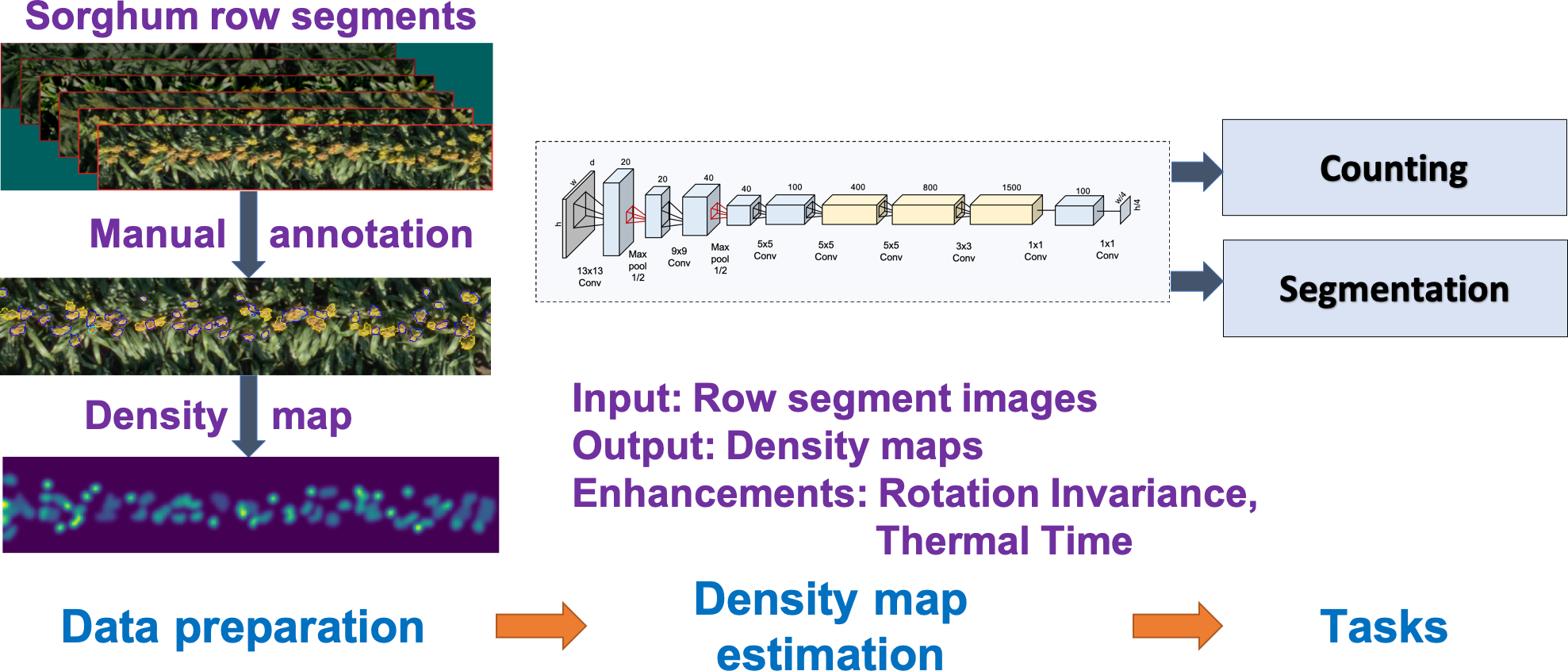
Figure 1: Overview of our proposed approach for counting and segmenting panicles of Sorghum.

1.1 Overview and Contributions

An overview of our system is provided in Figure 1. We first create superpixel sets of various sizes from the images to do human annotation to create the training data set. This annotation can be either dot-based or region-based. We create image density maps for counting using these annotations, and train a novel two-stage CNN architecture to predict these density maps. The proposed architecture includes methods to impose prior knowledge such as monotonicity in counts, and temperature dependence on the growth of the crop. The first stage is a panicle pixel detector that feeds into the second density estimator stage. Counts are obtained by integrating the density maps. Our proposed counting approach outperforms state-of-the-art systems such as CCNN [39], MCNN [58], and CSRNet [30] that are primarily applied to crowd counting. We then segment the individual panicle instances using a novel occlusion-aware clustering approach with the estimated density maps and detected panicle regions as inputs. Hence, the two outputs of our system is image level counts and the segmented individual panicle instances. The panicle instances can then be fed back to the annotation tool to accelerate human annotation. We consider our focus on Sorghum panicles to be an important contribution in this work, since it has the potential to directly impact crop breeding.

Some of the key challenges in counting and segmenting aerial Sorghum imagery include: (a) Dramatic differences in appearance between panicles. The appearance varies in size ($20\mathrm{cm}^{2}$ to $1000\mathrm{cm}^{2}$), shape (spindle, broom, cylinder or a lax cone), color (chalky white, green, yellow, rusty brown or black), pose, and grain-size, (b) self-occlusion of panicles later in the season, which is particularly severe with grassy varieties (see Appendix C). Hence, to develop a good panicle counting and segmentation system, we require a diverse, accurately annotated data set, and robust machine learning models trained on this data set, which is the main focus of this paper.

We obtain a mean absolute error (MAE) of $1.06$ compared to $1.19$ for the performance of a CSRNet model for counting panicles from aerial images of Sorghum. The instance segmentation model produces an mAP of $0.66$ at an IoU detection threshold of $0.5$. This nearly free instance segmentation can ultimately reduce the manual annotation workload for future data collection, by integration into the manual annotation tool.

We also obtained publicly available aerial imagery of Sorghum used for panicle counting [19]. Results with this data show that the deep counting methods, including the proposed counting regressor, outperform the methods proposed in [19] in a vast majority of cases.

In Section 2, we discuss the related work in counting and instance segmentation. Section 3 provides detailed description of the data and the steps involved in preparing it for modeling. Section 4 discusses the proposed approaches for counting along with counting experiments, while the proposed segmentation algorithm and the demonstration of its results is provided in Section 5.

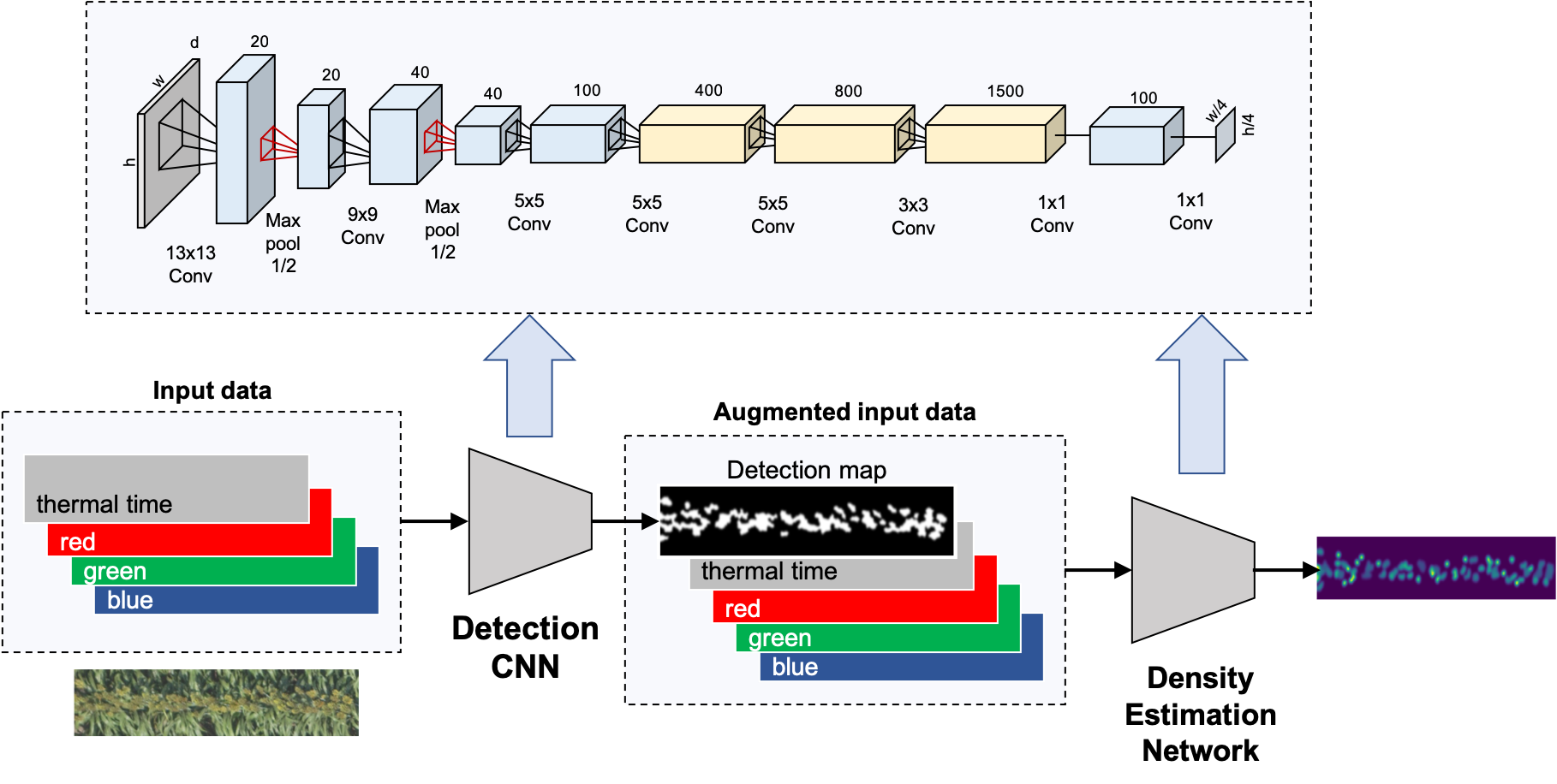
Figure 2: Proposed two-stage CNN architecture for density estimation for counting and segmentation of panicles.

2 Related Work

The problem of counting objects in images is seeing a resurgence with the advent of deep learning with applications in crowd and traffic monitoring, medical image analysis, and agronomy. The common challenge here is that manual counting can be laborious, inaccurate, and expensive.

Counting by detection is a 2-step process that first detects the objects then counts them. Counting by regression uses regression models, such as neural networks, with the object count as a target for the loss function [9]. In Counting by segmentation the image is segmented into foreground and background, and the counts are estimated from the foreground [21]. Recently proposed Detection by regression approaches [54, 53] attempt to reconstruct an image density map [28] as well as detect the cell in microscopy images. This is the closest to our proposed segmentation approach, however, our problem is much more complex since panicles are much more heterogeneous within and across the various varieties of Sorghum compared to cells that are mostly homogeneous in shape and appearance.

Most prevailing methods for counting use counting by regression approaches, where the non-linear regression function is represented by a CNN and the target is an image density map or the final count itself. However, some applications could use counting by detection or counting by segmentation if the detection or segmentation can be performed accurately. Depending on the problem, there is variation in the steps of the methodology such as estimating the density map from an annotation, the actual CNN architecture, and other enhancements involving semantic understanding of the counting problem. Some example application areas are in,

1. Crowd and Traffic Monitoring: Counting people in a crowd [50, 58, 46, 6] is perhaps the focus area of new counting approaches in many mainstream computer vision venues, and hence expanded in Section 2.1. There is also a good amount of literature on methods used for counting vehicles [10, 51, 12, 18].

2. Medical imaging: For general cell counting [55], cell counting and detection using fully convolutional regression networks [53], counting cells for images showing a developing human embryo [24], and counting bacteria colonies [16].

3. Agronomy: For general plant counting [43], counting palm trees [29], plant stalks [5], fruits [11, 40] and maize tassels [33]. This is a less mainstream application for counting, but a rich domain, that has real impact in people’s lives, and this will be the focus of our paper.

For agronomy applications, such as ours, understanding the crop is fundamental to developing an effective algorithm. A well executed counting by detection approach that illustrates this is [56] that count tomatoes by first segmenting the image then a decision tree extracts the fruit segments. The decision tree used color, shape, texture and size features to locate the tomatoes. A similar approach was taken in [19] for counting panicles in Sorghum. This is the only other published work we are aware of for panicle counting.

There is also a huge body of literature in instance segmentation, and we will discuss a few important and well-known ones here. A notable work is Mask R-CNN [20] proposed by He et al., which extends the well-known region proposal network, Faster R-CNN [42], by including a branch for predicting segmentation mask on each region of interest. In [27], the authors reduce the problem of instance segmentation to semantic segmentation to leverage the rich works in that area, by assigning colors to object instances. The information propagation in proposal based instance segmentation is boosted in [32] by enhancing the feature hierarchy with localization signals. An instance level segmentation approach for video is proposed in [23] that uses a recurrent neural net to take advantage of long-term temporal structures. An instance segmentation approach for neuronal cells in the brain using a hierarchical neural network was proposed in [57]. A refreshing mathematical approach for instance segmentation using semi-convolutional operators was proposed in [37]. To mitigate the labeling costs involved in instance segmentation, Hu et al. [22] propose a partially supervised paradigm to learn from a large set of categories that have box annotations where only a small fraction of them have mask annotations.

2.1 Crowd Counting

We review several architectures for crowd counting, since it is the main application area for counting in mainstream computer vision conferences. In this work, we reuse some of these architectures for comparisons.

In crowd counting, a key challenge is to build effective CNN architectures that handle perspective scale distortions. The central building block for several counting systems is the counting CNN (CCNN) [39] that we also use and fine-tune in our work. The CCNN, shown in Figure 14, is simply a deep CNN with an image density map as a regressor. A family of models have been developed that take an ensemble approach to the scale distortion problem. For the models in the family, the two main decisions that need to be made are: how to design the components in the architecture for the different head sizes, and how to combine these components.

A simple but elegant member of this family is the multi-column CNN (MCNN) [58], as seen in Figure 15, where the component models in the ensemble are CCNNs with the receptive fields in the convolutional kernel designed for a particular head size. The resulting CCNN predictors are then combined into one density map with a fully convolutional layer. The CCNN tends to over estimate the count when the density is very low and under estimate the count near the horizon line where the density is extremely high. This was used advantageously in the DecideNet model [31] where they noted that the counting by detection approach is particularly good when the density is very low. They then used another neural network to estimate an attention map and combine the two approaches.

While these papers used the CCNN type architecture, the popular U-net architecture has been used in [47] together with a scale consistency regularizer that forces collaborative predictions from the ensemble models. The U-net model has been widely used in medical imaging. E.g., Ronnenberger et al., [45] use the U-net for cell tracking in bio-medical imaging. Examples of works that allow for very deep networks include [48] and [30], both of which use a VGG [49] type architecture. Shi et al. [48] utilize a multi-scale architecture, where a part of their network uses complex ensemble averaging to combine image density maps from models built for different scales. Li et al. [30] introduce the dilated convolution to aggregate multi-scale contextual information in the CSRNet model (see Figure 16). [38] extended CSRNet by adding parallel branches for the last predictive layer. This allowed for uncertainty estimation as well as a way to improve the performance through ensemble averaging. Finally, it is worth mentioning the approach taken in [3] that first estimates the head size and position in order to choose the hyper parameters for the CCNN.

We have used the CCNN, MCNN and CSRNet models in our experiments, but it should be noted that none of these models achieve the best performance on the common crowd counting benchmarks. The CSRNet was the best performing model when published in CVPR 2018, but has since been surpassed on several benchmarks by SANet [52], ic-CNN [41] and by ASD [7]. Table 1 shows the performance of these 6 systems on the large and popular UCF CC 50 benchmark. The code for CCNN, MCNN and CSRNet have been released, but we are unaware of codes for SANet, ic-CNN, and ASD, which makes it almost impossible for us to make comparisons. We believe CSRNet is the best system for crowd counting that have been independently verified.

System	MAE	System	MAE
CCNN	488.7	ic-CNN	260.9
MCNN	377.6	SANet	258.4
CSRNet	266.1	ASD	196.2

Table 1: Performance for crowd counting for 6 systems on the UCF CC 50 benchmark.

All of these methods handle the problem of perspective by creating specialized models for heads of varying sizes. This will however degrade performance when all the human heads have the same size. In our application, the size of panicles varies through the season and by the variety, but we did not see any improvement in counting performance using the above approaches that compensate for perspective.

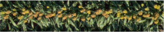
Figure 3: An example row-segment image.

3 Data and Preparation

In this section, we describe the RGB image data of Sorghum crops collected using unmanned aerial vehicles (UAVs) in 2017 at the experimental fields of Purdue University. These experiments are a part of our collaborative project in high-throughput phenotyping. This is the data using which we demonstrate our proposed approaches for counting and segmentation. We also describe our data preparation methodology. More details on the data are available in Appendix C.

More than 1000 varieties of sorghum were planted on the fields. We restrict our focus to a collection of plots named the hybrid calibration panel where 18 commercial Sorghum varieties were planted (see Appendix B). These 18 varieties were chosen to represent the variations from across the larger set. The hybrid calibration panel consisted of 88 rows that were divided into 20 ranges, and each image covered one row-segment corresponding to a particular row and range. Each of the 18 different varieties were planted on 4 plots, and each plot contained 12 consecutive row-segments on the same range. The 12 row-segments within each plot will be conveniently referred to as field rows, so that the first row-segment in a plot is field-row one, the second field-row two and so on. These row segments were extracted as described in [43]. As the panicle is the head of the plant it sits above the canopy and is visible by the UAV camera (See Figure 3).

We used images collected on $6$ different dates collected by UAVs that are roughly 1 week apart (7/11, 7/17, 7/25, 8/2, 8/8, and 8/16), and covered the full panicle development stage for most varieties of Sorghum. We used field rows 2 and 3 of each plot for these six dates (7/11-8/16) where no destructive phenotyping was performed. These $2\text{ rows}\times 4\text{ plots}\times 6\text{ dates}\times 18\text{ varieties}$, a total of $864$ row-segments were used in our panicle counting experiments. We also augmented the training data by considering rotations by 90, 180, 270 and 360 degrees as well as reflections for each rotation. This increases the size of the data set eight-fold, resulting in a total of $6,912$. An alternative to data augmentation is to use group equivariant networks [13, 14], but we stick to the simpler approach here.

All our experiments are performed using four way cross-validation, where we held out one plot for each variety for testing and trained on the rest, then rotated the held out plot until the entire data set was covered in the four test sets. The size of training and test sets for each cross-validation run would be $5,184$, and $1,728$ respectively. Finally, each row segment will have a unique result.

The main challenges with counting using the data are: (a) Dramatic differences in appearance between panicles. The appearance varies in size ($20\mathrm{cm}^{2}$ to $1000\mathrm{cm}^{2}$), shape (spindle, broom, cylinder or a lax cone), color (chalky white, green, yellow, rusty brown or black), pose, and grain-size, (b) self-occlusion of panicles later in the season, which is particularly severe with grassy varieties (see Appendix C). Hence, to develop a good panicle counting and segmentation system, we require a diverse, accurately annotated data set, and robust machine learning models trained on this data set.

3.1 Manual annotation

We developed a tool to perform region and dot annotation of panicles. Dot annotation consists of the user just clicking each panicle once. For region annotation, we start with a Simple Linear Iterative Clustering (SLIC) superpixel segmentation [1, 2], and a few clicks per panicle (in our application , about $3$) are needed for annotation. Our annotation tool provides for $3$ sizes of superpixels to allow the user to choose how accurately to annotate the panicles. Appendix E has an example image with the three corresponding superpixel segmentation sets. Our tool also incorporates a feedback mechanism, where it will ‘guess’ the panicle superpixels based on the current detection model, and the user only has to correct its predictions. This feedback loop becomes quite helpful for accelerating human annotation as well as model training.

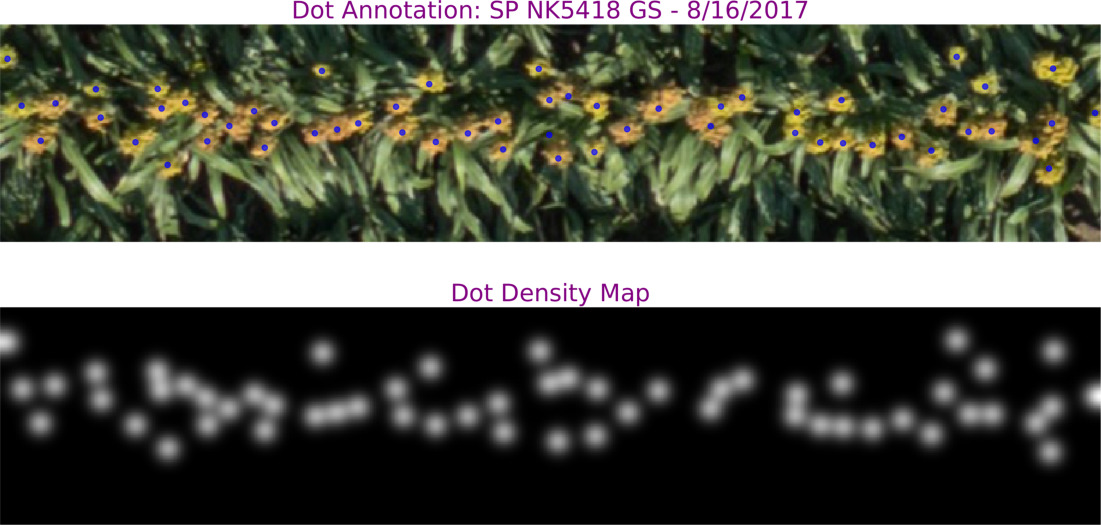
Figure 4: Example dot annotation and corresponding dot density map.

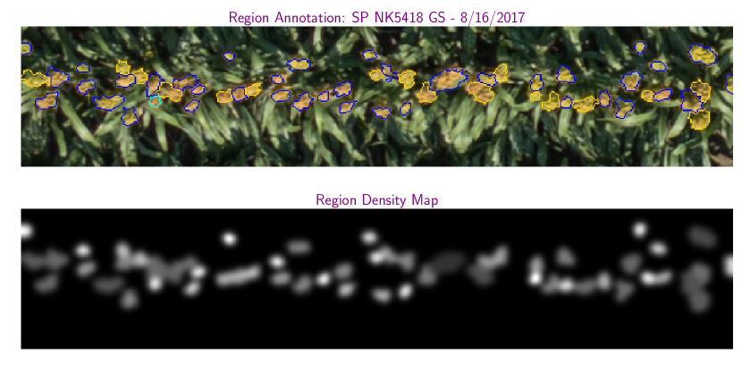
Figure 5: Example region annotation and corresponding region density map.

The total number of panicles in all the images is 12,099. The annotated panicles corresponded to 35,329 superpixels for region annotation. We give some examples of easy and hard to annotate images in Appendix C.

3.2 Image Density Map Estimation

The target for our regression network is density maps derived from annotations of panicle images. From the dot and region annotations, we respectively derive the dot and the region density maps. In the dot density map, we start with an indicator map that denotes the location of each panicle with a dot, and convolve a fixed width Gaussian kernel with it. This can be seen in Figure 4. In the region density map, the user annotates the entire region of the panicle. The area under each distinct panicle region sums to 1. This is convolved with a small fixed width Gaussian (see Figure 5). For each of these density maps the total density equals the number of panicles in the image. The counting performance in using dot vs. region annotation was almost the same. However, the predicted dot density maps are also ideal for locating the center of the panicle, while the predicted region density map indicates the full extent of a panicle. The region density maps are also used along with the proposed instance segmentation approach, and this is lot harder to achieve with dot density maps.

4 Proposed Counting Regressor

Due to one third of the images containing none or very few panicles, the CCNN, MCNN and CSRNet models (see Appendix D for the architecture diagrams) do not train properly on our data set. In most training runs the model eventually converges to zero due to the nature of the data. Adding a batch normalization layer after every convolutional layer fixed this issue and allowed all the models to be trained on our data set. Conversely, adding batch normalization to the crowd counting data did not improve the performance. This meant initializing CSRNet with VGG16_bn – a version of VGG16 with batch normalization.

Our proposed counting regressor was a tuned version of the CCNN approach [39] that has different number of layers and convolutional filter sizes. To enable training from small data sets, with only hundreds of images, it is necessary to use an intermediate lifted high dimensional target. We use the image density map that distributes the count as a unit density for each panicle. Since our images only has small perspective distortions, we found that we do not need more complex architectures such as MCNN. In fact, the more complex architectures tend to hurt the performance, as we added enhancements to the CNN models.

The architecture we employed is shown in Figure 2. We experimented with various choices of hyper parameters of the network, such as the number of layers, the size of the receptive filters or convolutional kernels (kernel), and the number of output channels (dim). For the canonical CCNN we had dim=[32, 32, 32, 1000, 400, 1], kernel=[7, 7, 3, 1, 1, 1], whereas our best model used dim=[20, 40, 100, 400, 800, 1500, 100, 1], kernel=[13, 9, 5, 5, 5, 3, 1, 1]. It was beneficial to make the number of filters be 1 for the last layer(s) so as to get a fully connected convolutional layer. The network had two max pooling layers inserted before the second and third convolutional layers. As the max-pooling reduces the size of the output, the resulting image density map had to be down-sampled accordingly. This problem can be potentially overcome using fully convolutional regression networks [53].

We additionally enhanced our system, CCNN, MCNN and CSRNet through four separate mechanisms. First, we encode rotation and reflection invariance through median averaging of the CNN predictions. Secondly, we use thermal time [44] as a proxy to encode the plant developmental stages. Thirdly, the time series of panicle count predictions is forced to monotonically increase through the use of isotonic regression [15]. Finally we used a panicle pixel detection map as an added input channel to the CNNs. This detection map was generated using the system in Figure 2 and as this system is quite accurate no noticeable difference was seen when using another CNN architecture to produce the detection map.

These enhancements are described in the rest of this section, and the corresponding results are included in Table 2.

4.1 Rotational Invariance

Similar to training data augmentation, we also rotate and flip the data at test time and then use a statistic of all the predictions to create an invariant prediction. Both the mean and median are candidates for the invariant statistics, but we found the median to be the superior choice as it consistently yielded slightly better results due to its robustness to outliers.

4.2 Isotonic Regression

The number of panicles should be a monotonically increasing function with time short of a drastic event (water lodging, diseases, extreme weather). In fact this growth curve is roughly sigmoidal [4]. Modelling errors on the other hand frequently lead to non-monotonic behavior as can be seen in the middle plot in Figure 6. Correcting these anomalies should lead to improved performance.

Isotonic regression [8, 15] forces the count to be non-decreasing through the least squares minimization

$$\min_{c_{i}}\sum_{i=1}^{n}\|c_{i}-\hat{c}_{i}\|_{2}^{2}\text{ subject to }c_{1}\leq c_{2}\leq\cdots\leq c_{n},$$ (1)

where $\hat{c}_{i}$ is the count estimates and $c_{i}$ is the desired monotonic correction. We use the efficient pool adjacent-violators algorithm (PAVA) [34], implemented in Python’s scikit-learn library to solve (1). Figure 6 shows the human annotation derived counts, the CNN predictions and the isotonic corrections side by side for one of the 18 varieties. In Appendix F, we show these results for our best system on all varieties.

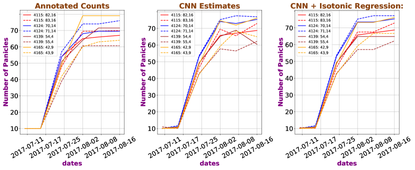
Figure 6: Panicle predictions for all annotated row segments of the variety SP NK5418 GS. Rows on different plots are in different colors. The numbers in the legend are respectively the plot and the $x,y$ identifier of the row-segment. The left plot shows counts from the human annotation, the middle figure shows predictions with the region density map CNN with median averaging. The right plot shows the isotonic regression derived from the middle plot.

4.3 Thermal Time

As the plant develops it eventually reaches a stage where panicles appear for some time until they are fully developed. The temperature is a very important factor in plant development [44] - a plant is stressed when it is cold and grows faster when it is warm. The plant development correlates well with the thermal time, measured as growing degree days (GDD). Specifically for Sorghum, we define the GDD as the number of degree days above $50^{\circ}\mathrm{F}$ since planting. With this definition a short season hybrid for example needs on average $1848^{\circ}\mathrm{F}$ to reach flowering. Using the thermal time in place of the time of the year also allows us to use the same model in a different location or for a different year. There are many ways to provide the thermal time to the CNN, but we provided it as a separate channel for the image as in Figure 2.

4.4 Detection Map

We used our CCNN like system with dim=[20, 40, 100, 400, 800, 1500, 100, 1], kernel=[13, 9, 5, 5, 5, 3, 1, 1] with the binary panicle pixel mask as a regressor. We refer to the predicted mask with values ranging from 0-1 as the detection map and added it to the input data channels. The detection map as well as the thermal time allows the CNN models to ignore the parts of the images that do not contain panicles. This results in the models effectively being trained on a much smaller data set, which meant that more complex models saw less benefit (if any) from these added channels.

4.5 Experimental Results

Table 2 shows the results for the CCNN, MCNN, CSRNet and our own tuned version of the CCNN architecture. It can be seen that the models with the largest number of parameters are MCNN and CSRNet and they do not see nearly the same gain as the smaller models when adding the thermal and panicle detection channels. CSRNet in particular sees no gain despite being smaller than MCNN. This is due to CSRNet being a much deeper architecture that suffers from a larger degree of over training (as discussed in [30]). We observed that the mean absolute error for the CSRNet model is 0.29 for training data vs. 1.19 on test data for the region density model. The new channels allows CSRNet to effectively focus on only the panicle data (less than 2% of the image data), so the over training data is exacerbated. Our model with all the bells and whistles gives an MAE of 1.06 compared to 1.17 for the plain CSRNet model - a relative improvement of nearly 10%. We expect that as the amount of annotated data increases the larger models will also benefit from the thermal and detection map channels.

System	Size	Base	+Rot	+Isot	+ther	+det	Base	+Rot	+Isot	+ther	+det
		region					dot
CCNN	2MB	1.52	1.46	1.38	1.26	1.14	1.62	1.53	1.39	1.33	1.11
Ours	21MB	1.38	1.36	1.28	1.17	1.08	1.39	1.38	1.28	1.18	1.06
MCNN	86MB	1.43	1.37	1.29	1.29	1.21	1.38	1.38	1.28	1.25	1.24
CSRNet	62MB	1.19	1.14	1.11	1.09	1.10	1.17	1.12	1.09	1.10	1.11

Table 2: CNN prediction errors for counting with various enhancements. We use the abbreviations ”Rot” for rotational invariance, ”Isot” for isotonic regression, ”ther” for thermal time and ”det” for detection map.

4.6 Results on Publicly Available Data

The only publicly available data we are aware of for counting panicles in Sorghum aerial imagery was released with [19] by Guo et al. In this section, we provide a brief description of the dataset, and also the results for counting using our proposed regressor.

Guo et al.’s data contains a training set of 40 large images with roughly 105 panicles in each image and two test sets. The test sets are referred to as dataset 1 and dataset 2. Dataset 1 has 489 panicles per image on average, while dataset 2 typically has 106 panicles per image on average. The resolution is higher than for our images (0.45cm $\times$ 0.45cm per pixel versus 0.66cm $\times$ 0.66cm per pixel).

The data is all from one date, so we cannot take advantage of the thermal time or isotonic regression that gave us some gain in performance. Also, experiments using a detection layer as an input channel did not yield gain in performance. We do not know exactly why this is, but suspect that both the region density map as well as the detection map are less effective due to the larger extent of each panicle resulting from the increase in resolution. Also, we do not know the accuracy of the pixel detection density map as the test sets were only annotated in terms of panicle centers. Table 3 gives the results for our proposed counting regressor model, CCNN, MCNN and CSRNet. CSRNet is superior to the other methods and perhaps the reason is that the dilated convolutions gives the model a bigger effective receptive field – hence the ability to grapple with the larger extent of the panicles. In [19] the authors do not report MAE, but rather report the coefficient of determination $R^{2}$. We give $R^{2}$ results to compare with their results in Table 4.

System	Density	Dataset 1		Dataset 2
		Base	+rot	Base	+rot
CCNN	dot	21.67	22.94	5.00	4.24
	region	19.56	19.37	4.16	4.10
Ours	dot	20.39	19.52	3.23	3.15
	region	23.64	23.46	3.56	3.66
MCNN	dot	20.61	20.14	3.72	3.29
	area	22.52	23.85	3.16	3.32
CSRNet	dot	17.12	16.70	2.72	2.20
	region	21.32	20.82	3.84	3.57

Table 3: MAE on the two test sets released with [19] for four different CNN architectures for counting.

System	Density	Dataset 1		Dataset 2
		Base	+rot	Base	+rot
Quadratic SVM [19]	-	0.84		0.56
CCNN	dot	0.88	0.86	0.52	0.61
	region	0.86	0.86	0.63	0.65
Ours	dot	0.90	0.90	0.77	0.80
	region	0.85	0.84	0.80	0.82
MCNN	dot	0.81	0.80	0.73	0.79
	region	0.64	0.57	0.79	0.76
CSRNet	dot	0.89	0.90	0.86	0.88
	region	0.84	0.85	0.73	0.75

Table 4: Coefficient of determination, $R^{2}$, on the two test sets released with [19] for four different CNN architectures for counting as well as the Quadratic SVM method proposed in [19].

5 Panicle Detection and Segmentation

The size and shape of a panicle is by itself an interesting phenotype, but to derive this information we need to move beyond the count and estimate a panicle instance segmentation indicating which pixels belongs to each panicle versus the background. We propose a novel instance segmentation approach wherein we: (a) use the image detection map to directly detect panicle superpixels, and (b) group superpixels into panicle segments using clustering and the region density map. Early in the growth season, when there is no occlusion, segmentation can be done through the connected components from the panicle detection map. The late season images can have severe occlusion problems - especially for grassy varieties - and the difficulty is increased by overlapping panicles with homogeneous texture and few discernible edges. We use the fact that the integrated density over a particular panicle should equal $1$ and rely on the region density map to extract individual panicles. We then perform density aware greedy clustering to obtain panicle segments.

5.1 Detecting Panicle Superpixels

In order to have efficient algorithms we cluster superpixels in place of pixels. We used the CNN in Figure 2 with the panicle detection map as a regressor. At test time this CCNN model will predict a detection map, thus acting as a panicle pixel detector (see Appendix A for more details). The predicted detection map can be interpreted as an estimated pixel panicle probability. To convert this into a superpixel panicle detector we used the mean panicle pixel probability as the superpixel panicle probability. We set a probability threshold $\alpha$ as a detection threshold and varied $\alpha$ between 0.3 and 0.6 to affect the precision-recall balance. The panicle superpixel detector algorithm is given in Algorithm 1. Note that $S$ is the superpixel map (matrix) that assigns a pixel to a superpixel value.

Input: thermal time tt, image $I$

Output: Set of panicle superpixels $P$

$D=\mathrm{detection\_CNN}(\texttt{tt},I)$

/* $D(i,j)=$ panicle pixel probability. */

$S=\mathrm{SLIC}(I)$

  // $S(i,j)=t$ for superpixel $t$.

$$P=\left\{p:\frac{\sum_{ij:S(i,j)=p}D(i,j)}{\sum_{ij:S(i,j)=p}1}\geq\alpha\right\}$$

Algorithm 1 Panicle Superpixel Detector

5.2 Cluster Fitness

Discovering which superpixels belong to a single panicle is difficult in the presence of occlusion as they have the texture and color tends to be the same. This leads us to focus the objective on the shape-compactness and to depend to a large degree on the region density map. This lead us to use the definition of cluster fitness defined in Algorithm 2. Many clustering algorithms are distance based (K-means, DBSCAN, Agglomerative Clustering), but can also be formulated in terms of cluster fitness. Our cluster fitness is a weighted combination of how small the cluster variance is and how close the total cluster density mass is to $\beta$. $\beta$ should ideally be 1, but we change it to vary the number of recovered panicles for the precision-recall curve. $C$ in the algorithm is a map from superpixel panicle indices to clusters.

Input: cluster $c$, $\beta$, superpixel map $S$, tt, cluster assignment $C$

Output: cluster fitness $f$

$R=\mathrm{region\_CNN}(\texttt{tt},I)$

  // Region density map

for $i,j$ do

       /* $v$ - vectors for clustering pixels */

       $v(i,j):=[\gamma i,\gamma j,\mathrm{red},\mathrm{green},\mathrm{blue}]$

        // $\gamma=10$

      

$n=\sum_{i,j:C(S(i,j))=c}1$

  // pixel count

mean = $\frac{1}{n}\sum_{i,j:C(S(i,j))=c}v(i,j)$

var = $\frac{1}{n}\sum_{i,j:C(S(i,j))=c}(v(i,j)-\mathrm{mean}(c))^{2}$

$d=\sum_{i,j:C(S(i,j))=c}R(i,j)$

  // density mass

$f=n(\delta(d-\beta)^{2}+\mathrm{var})$

  // $\delta=46775$, $\beta\approx 1$.

return $f$

Algorithm 2 Cluster Fitness

5.3 Instance Segmentation

To discover the individual panicle segments we used greedy bottom-up clustering. Initially every panicle superpixel is its own cluster. We then progressively merge pairs of clusters until the accumulated cluster fitness is increased. At each step the pair with the best cluster fitness change is identified for the merge. Algorithm 3 shows the details. A result of this clustering process can be seen in Figure 7.

Input: $P$, $\beta$, $S$, tt

Output: clusters $C$

$C=P$

  // All superpixels are clusters

$\mathrm{loss}=-1$

while $\mathrm{loss}<0$ do

       $B=(0,0,0)$

       for $c_{1}\neq c_{2}\in\mathrm{set}(C)$ do // find best merge

             if $\mathrm{connected}(c_{1},c_{2})$ then

                   /* cost of merging $c_{1}$ and $c_{2}$ */

                   $\mathrm{loss}=\mathrm{fitness}(c_{1},c_{2})-\mathrm{fitness}(c_{1})-\mathrm{fitness}(c_{2})$

                   if $\mathrm{loss}<B(0)$ then

                         $B=(\mathrm{loss},c_{1},c_{2})$

                  

            

      $\mathrm{loss},c_{1},c_{2}=B$

       if $\mathrm{loss}<0$ then

             for $p\in P$ do // merge $c_{1},c_{2}$

            

                   if $C(p)==c_{2}$ then

                         $C(p)=c_{1}$

                  

            

      

return $C$

Algorithm 3 Instance Segmentation

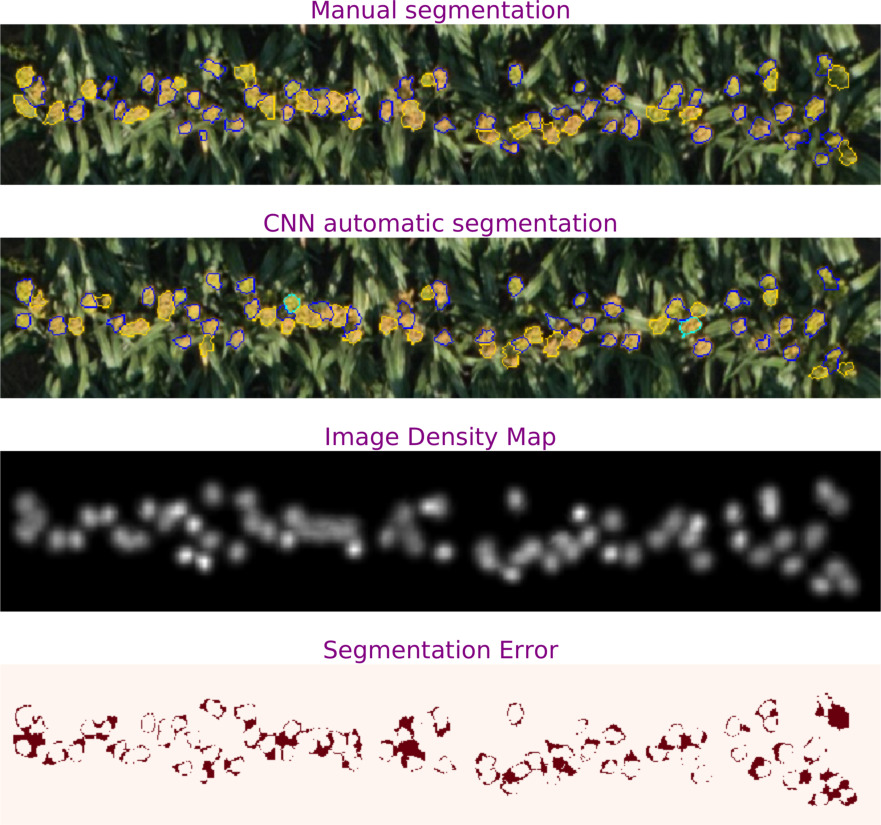
Figure 7: A comparison of the manual and automatic segmentation.

Computing the Intersection of Union (IoU) for instance segmentation not based on rectangle annotation is more involved. To compute the IoU requires first an alignment procedure so as to not allow one panicle to correspond to two panicles in the annotation. This problem is known as a transportation or assignment problem and can be solved with the Hungarian algorithm also known as the Kuhn–Munkres algorithm or Munkres assignment algorithm [25, 26, 36]. We varied $\alpha$ and $\beta$ (Algorithm 3) to compute a precision-recall curve from which we derive the mAP to be 0.66 for a detection threshold of IoU=0.5. The performance of our instance segmentation procedure is bounded by the quality of the region segmentation system and it is possible to obtain better performance using a specialized approach. However, our methodology is extremely efficient and compatible with our counting algorithm. It can also be accessed real time in a GUI and requires little additional code once a counting CNN is provided.

Appendix A Segmentation Using a Panicle Detection CNN

In order to paint a complete and fair picture we have to describe the CNN detection system. We trained a CNN with the same architecture as the CCNN where the density map regression targets were replaced with a detection map. Our detection map was a smooth version of the binary foreground-background indicator constructed by convolving against a fixed width gaussian the same way we did for the density map. We see an example detection map in Figure 8.

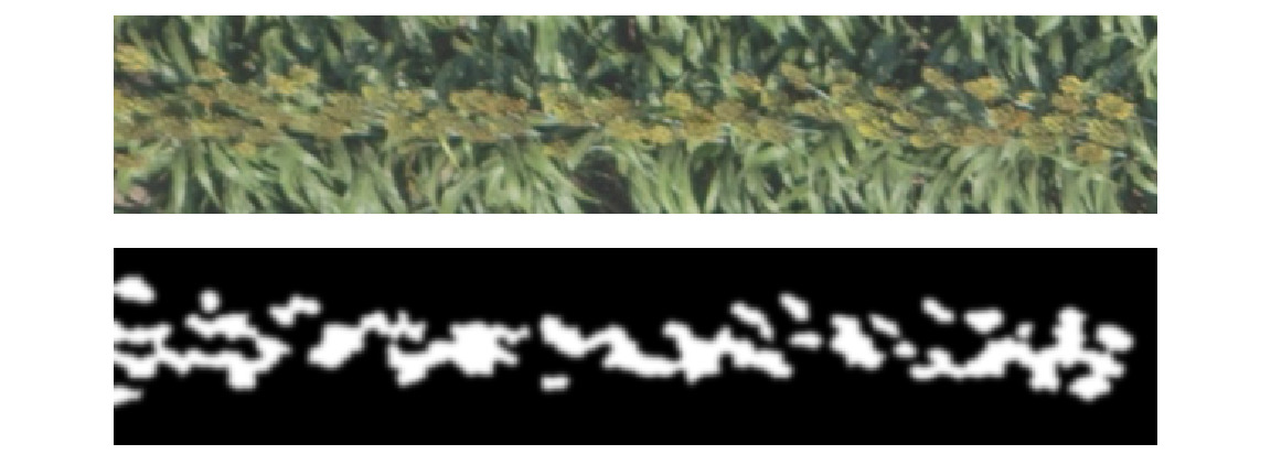
Figure 8: An example regression target for the panicle detection CNN model.

Appendix B Sorghum Pedigrees

The data collected consisted of images of the Hybrid Calibration Panel where the 18 hybrid varieties of sorghum listed in Table 5 were grown.

Pedigree
PH 849F FS
PH 877F FS
RS 327x36 BMR FS
RS 341x10 FG white
RS 366x58 FG white
RS 374x66 FS
RS 392x105 BMR FS
RS 400x38 BMR SG
RS 400x82 BMR SG
SP HIKANE II FS
SP NK300 FS
SP NK5418 GS
SP NK8416 GS
SP SS405 FS
SP Sordan 79 FS
SP Sordan Headless FS PS
SP Trudan 8 FS
SP Trudan Headless FS PS

Table 5: List of the 18 sorghum pedigrees grown in the 2017 hybrid calibration panel.

Appendix C Examples Images

Figure 9 shows images over a row segment for the variety SP NK5418 GS for the six dates the UAV was flown. Note that there is significant variations across the dates even though the variety is the same.

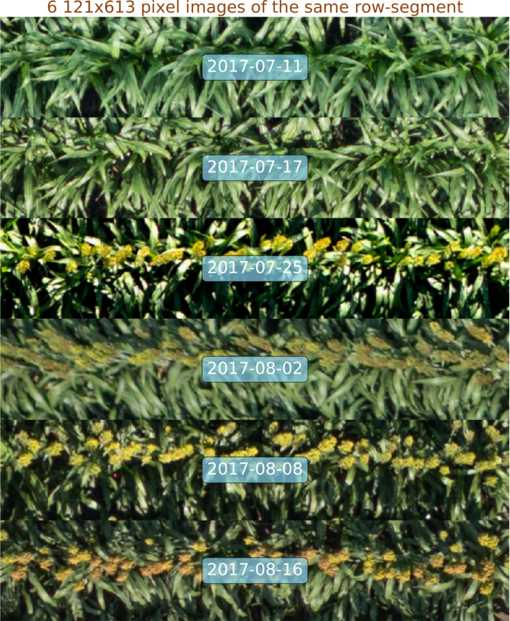
Figure 9: Example Sorghum UAV images from the 2017 hybrid calibration panel.

The 2017 hybrid calibration data contained a mix of images, some of which were easy and some of which were hard to annotate. Figure 11 show some example row-segment images in the data that exemplified the different problems encountered when trying to annotate the data.

Figure 10 shows two varieties of sorghum where the panicle sizes are quite different. The second image also demonstrates how dramatic the self-occlusion can be in the grass-like varieties of sorghum.

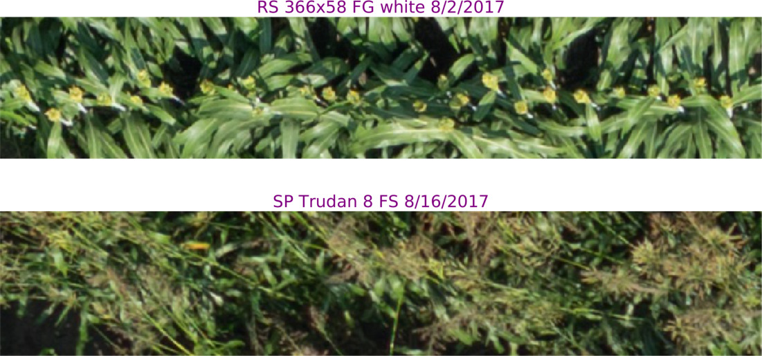
Figure 10: Example of panicle size variation.

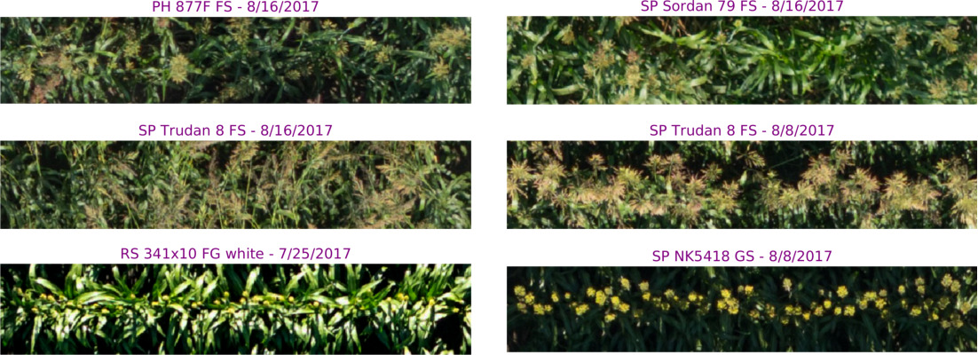
Figure 11: Example row-segment images where it is harder to annotate and count the panicles.

Figure 12 shows a concrete example of an image, the group of rotations by 90 degrees and flips and the corresponding predictions.

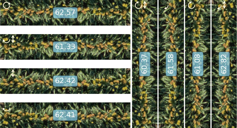
Figure 12: An example of the CNNs predictions for flips and rotations for one image. The manual human count was 57 for this image, while the median statistics gave 61.99 and the mean statistics gave 61.82. The arrows indicate the rotation and the up down arrows a vertical flip.

Figure 13 shows an image representation of all manually annotated panicles on 8/16/2017 on the hybrid calibration plot. There were a total of 4501 panicles observed on the last date and these represent 17 out of the 18 varieties as heads of one variety only appeared in September.

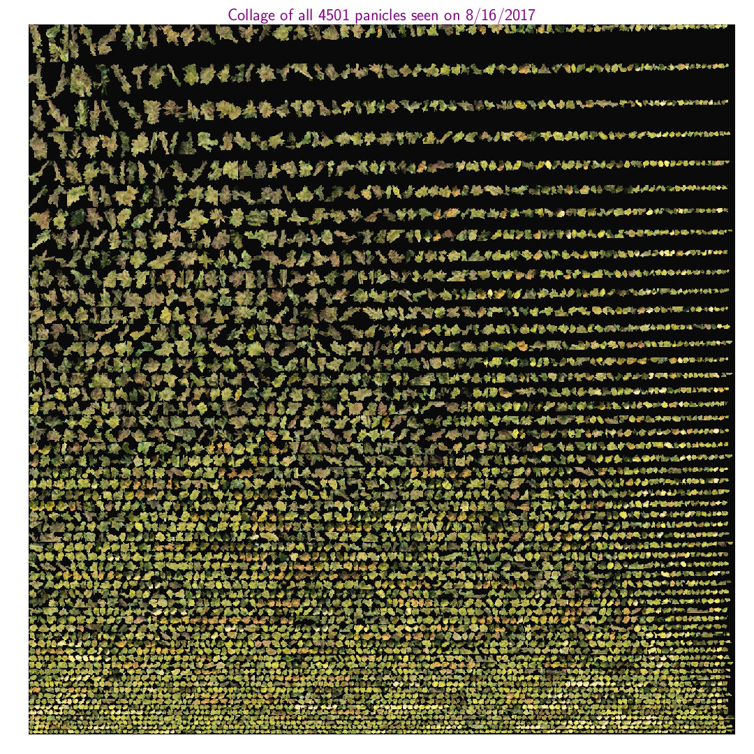
Figure 13: A collage of all 4501 panicles seen on 8/16/2017.

Appendix D CNN Architectures

In this section we show the competing CNN architectures. Figure 14 shows the original Counting CNN (CCNN) network in [39]. Figure 15 shows the Multi-column CNN network (MCNN). MCNN consists of 3 columns of CCNN-like structure where the convolutional kernel sizes are fixed at 3, 5 and 7 respectively. Finally, Figure 16 shows CSRNet that consists of the first 10 layers of the VGG-16 model. We refer to this as the front-end. The back-end consists of 6 layers with dilated convolutional kernels to estimate the image density map.

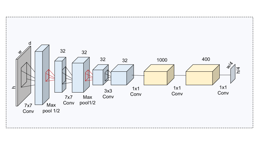
Figure 14: The CCNN architecture.

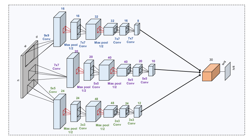
Figure 15: The MCNN architecture

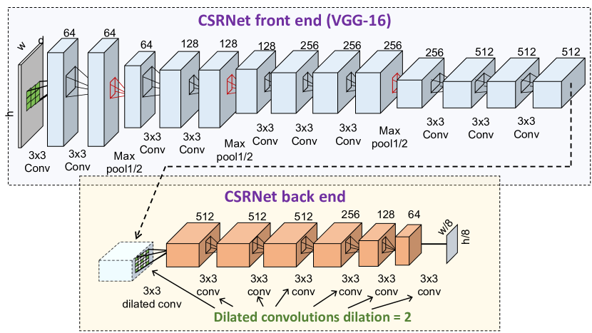
Figure 16: The CSRNet architecture

Appendix E Superpixel Segmentation

Figure 17 shows an example image along with three sets of superpixels used in the annotation tool. We denoted the three sets small, medium and large superpixels in which the average superpixel size was respectively 30, 60 and 110 pixels. The advantage of having these three segmentation sets is two-fold in both speed and accuracy of the annotation. Firstly, it allows the annotator to save time by using the segmentation set whose superpixel sizes matches the panicle size most closely. Secondly, having three independently made segmentation sets allow us to switch the segmentation set when the alignment to the actual panicles do not match the selected segmentation set.

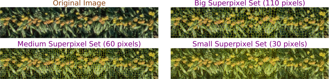
Figure 17: An image and three levels of superpixel segmentation with average size of 30, 60 and 110 pixels.

Appendix F Results From Best Model

The plots in Figure 18-23 contains the counts and the predicted counts with and without isotonic regression for our best system (with MAE=1.17). It can be seen that several of the varieties had very few panicles at all. These varieties were photo-sensitive and only flowered when the days became shorter and we have no image from that part of the growing season.

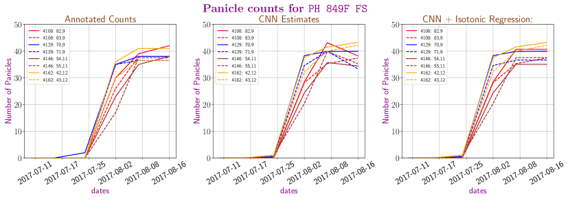
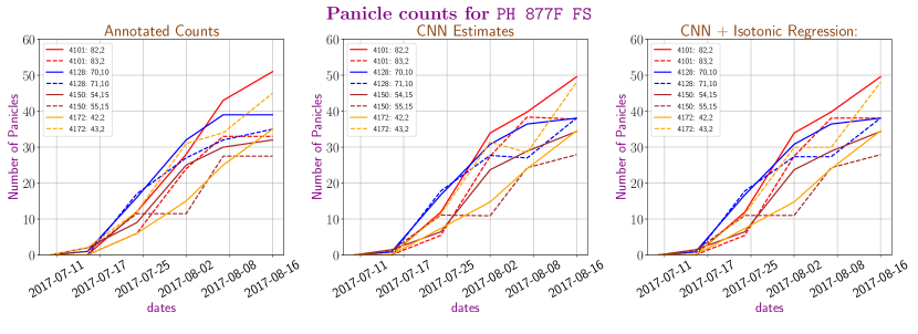
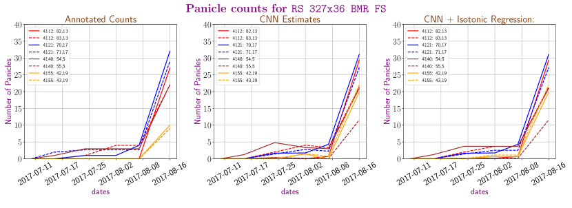
Figure 18: Manual panicle counts and CNN prediction counts with and without isotonic regression for the best CNN system for the three varieties PH 849F FS, PH 877F FS and RS 327x36 BMR FS.

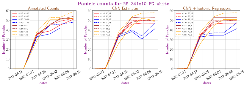
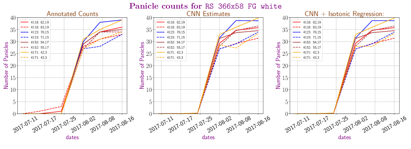
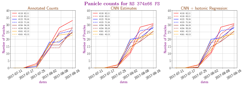
Figure 19: Manual panicle counts and CNN prediction counts with and without isotonic regression for the best CNN system for the three varieties RS 341x10 FG white, RS 366x58 FG white and RS 374x66 FS.

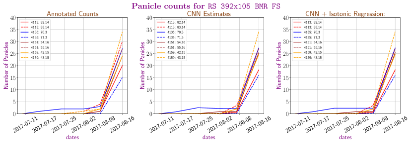
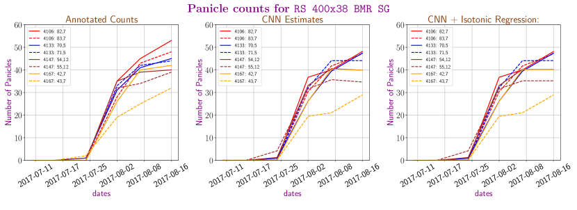
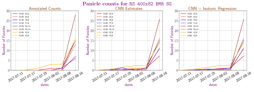
Figure 20: Manual panicle counts and CNN prediction counts with and without isotonic regression for the best CNN system for the three varieties RS 392x105 BMR FS, RS 400x38 BMR SG and RS 400x82 BMR SG.

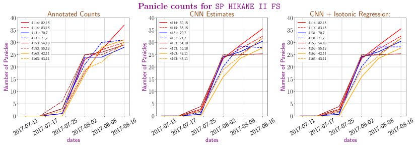
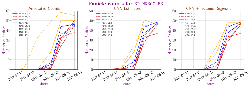
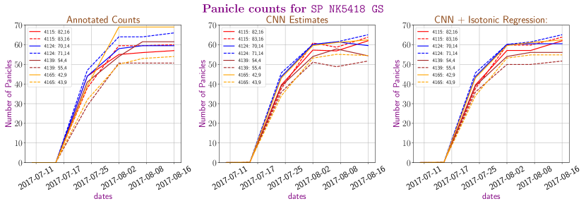
Figure 21: Manual panicle counts and CNN prediction counts with and without isotonic regression for the best CNN system for the three varieties SP HIKANE II FS, SP NK300 FS and SP NK5418 GS.

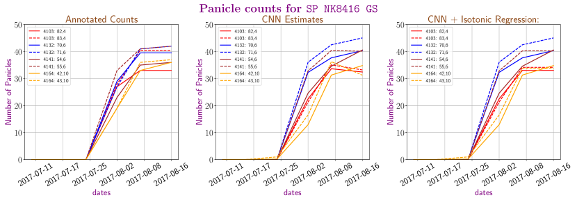
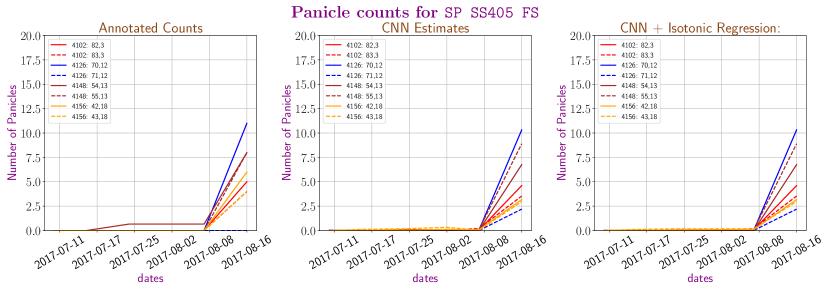
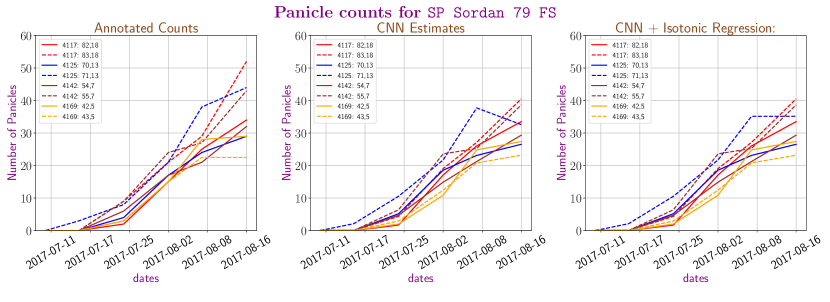
Figure 22: Manual panicle counts and CNN prediction counts with and without isotonic regression for the best CNN system for the three varieties SP NK8416 GS, SP SS405 FS and SP Sordan 79 FS.

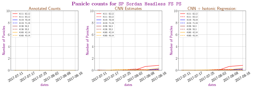
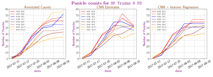
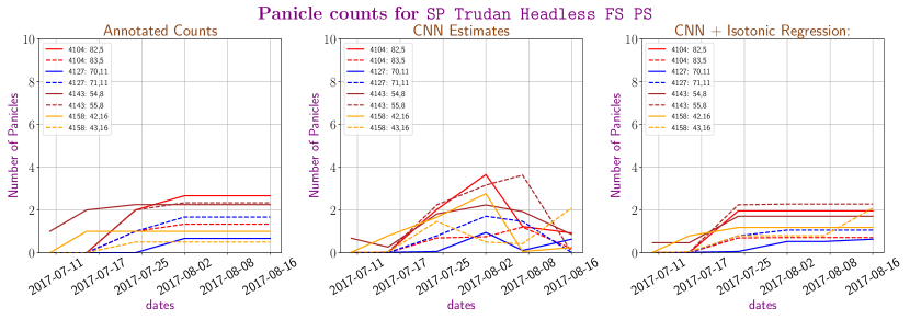
Figure 23: Manual panicle counts and CNN prediction counts with and without isotonic regression for the best CNN system for the three varieties SP Sordan Headless FS PS, SP Trudan 8 FS and SP Trudan Headless FS PS.

References

- [1] R. Achanta, A. Shaji, K. Smith, A. Lucchi, P. Fua, and S. Süsstrunk. SLIC superpixels. Technical report, 2010.
- [2] R. Achanta, A. Shaji, K. Smith, A. Lucchi, P. Fua, and S. Süsstrunk. SLIC superpixels compared to state-of-the-art superpixel methods. IEEE transactions on pattern analysis and machine intelligence, 34(11):2274–2282, 2012.
- [3] S. Amirgholipour, X. He, W. Jia, D. Wang, and M. Zeibots. A-CCNN: Adaptive CCNN for density estimation and crowd counting. In 2018 25th IEEE International Conference on Image Processing (ICIP), pages 948–952. IEEE, 2018.
- [4] A. Bartel and J. Martin. The growth curve of sorghum. J. Agric. Res, 57:843–849, 1938.
- [5] H. S. Baweja, T. Parhar, O. Mirbod, and S. Nuske. StalkNet: A deep learning pipeline for high-throughput measurement of plant stalk count and stalk width. In Field and Service Robotics, pages 271–284. Springer, 2018.
- [6] L. Boominathan, S. S. Kruthiventi, and R. V. Babu. Crowdnet: A deep convolutional network for dense crowd counting. In Proceedings of the 2016 ACM on Multimedia Conference, pages 640–644. ACM, 2016.
- [7] X. Cao, Z. Wang, Y. Zhao, and F. Su. Scale aggregation network for accurate and efficient crowd counting. In Proceedings of the European Conference on Computer Vision (ECCV), pages 734–750, 2018.
- [8] N. Chakravarti. Isotonic median regression: a linear programming approach. Mathematics of operations research, 14(2):303–308, 1989.
- [9] A. B. Chan and N. Vasconcelos. Counting people with low-level features and bayesian regression. IEEE Transactions on Image Processing, 21(4):2160–2177, 2012.
- [10] M. S. Chauhan, A. Singh, M. Khemka, A. Prateek, and R. Sen. Embedded cnn based vehicle classification and counting in non-laned road traffic. In Proceedings of the Tenth International Conference on Information and Communication Technologies and Development, page 5. ACM, 2019.
- [11] S. W. Chen, S. S. Shivakumar, S. Dcunha, J. Das, E. Okon, C. Qu, C. J. Taylor, and V. Kumar. Counting apples and oranges with deep learning: a data-driven approach. IEEE Robotics and Automation Letters, 2(2):781–788, 2017.
- [12] J. Chung and K. Sohn. Image-based learning to measure traffic density using a deep convolutional neural network. IEEE Transactions on Intelligent Transportation Systems, 19(5):1670–1675, 2018.
- [13] T. Cohen and M. Welling. Group equivariant convolutional networks. In International conference on machine learning, pages 2990–2999, 2016.
- [14] T. S. Cohen, M. Geiger, J. Köhler, and M. Welling. Spherical CNNs. arXiv preprint arXiv:1801.10130, 2018.
- [15] J. De Leeuw. Correctness of kruskal’s algorithms for monotone regression with ties. Psychometrika, 42(1):141–144, 1977.
- [16] A. Ferrari, S. Lombardi, and A. Signoroni. Bacterial colony counting by convolutional neural networks. In Engineering in Medicine and Biology Society (EMBC), 2015 37th Annual International Conference of the IEEE, pages 7458–7461. IEEE, 2015.
- [17] R. T. Furbank and M. Tester. Phenomics – technologies to relieve the phenotyping bottleneck. Trends in Plant Science, 16(12):635 – 644, 2011.
- [18] R. Guerrero-Gómez-Olmedo, B. Torre-Jiménez, R. López-Sastre, S. Maldonado-Bascón, and D. Onoro-Rubio. Extremely overlapping vehicle counting. In Iberian Conference on Pattern Recognition and Image Analysis, pages 423–431. Springer, 2015.
- [19] W. Guo, B. Zheng, A. B. Potgieter, J. Diot, K. Watanabe, K. Noshita, D. R. Jordan, X. Wang, J. Watson, S. Ninomiya, et al. Aerial imagery analysis–quantifying appearance and number of sorghum heads for applications in breeding and agronomy. Frontiers in plant science, 9, 2018.
- [20] K. He, G. Gkioxari, P. Dollár, and R. Girshick. Mask r-cnn. In Proceedings of the IEEE international conference on computer vision, pages 2961–2969, 2017.
- [21] C. X. Hernández, M. M. Sultan, and V. S. Pande. Using deep learning for segmentation and counting within microscopy data. arXiv preprint arXiv:1802.10548, 2018.
- [22] R. Hu, P. Dollár, K. He, T. Darrell, and R. Girshick. Learning to segment every thing. In Proceedings of the IEEE Conference on Computer Vision and Pattern Recognition, pages 4233–4241, 2018.
- [23] Y.-T. Hu, J.-B. Huang, and A. Schwing. Maskrnn: Instance level video object segmentation. In I. Guyon, U. V. Luxburg, S. Bengio, H. Wallach, R. Fergus, S. Vishwanathan, and R. Garnett, editors, Advances in Neural Information Processing Systems 30, pages 325–334. Curran Associates, Inc., 2017.
- [24] A. Khan, S. Gould, and M. Salzmann. Deep convolutional neural networks for human embryonic cell counting. In European Conference on Computer Vision, pages 339–348. Springer, 2016.
- [25] H. W. Kuhn. The hungarian method for the assignment problem. Naval research logistics quarterly, 2(1-2):83–97, 1955.
- [26] H. W. Kuhn. Variants of the hungarian method for assignment problems. Naval Research Logistics Quarterly, 3(4):253–258, 1956.
- [27] V. Kulikov, V. Yurchenko, and V. Lempitsky. Instance segmentation by deep coloring. arXiv preprint arXiv:1807.10007, 2018.
- [28] V. Lempitsky and A. Zisserman. Learning to count objects in images. In Advances in neural information processing systems, pages 1324–1332, 2010.
- [29] W. Li, H. Fu, L. Yu, and A. Cracknell. Deep learning based oil palm tree detection and counting for high-resolution remote sensing images. Remote Sensing, 9(1):22, 2016.
- [30] Y. Li, X. Zhang, and D. Chen. CSRNet: Dilated convolutional neural networks for understanding the highly congested scenes. In Proceedings of the IEEE Conference on Computer Vision and Pattern Recognition, pages 1091–1100, 2018.
- [31] J. Liu, C. Gao, D. Meng, and A. G. Hauptmann. DecideNet: counting varying density crowds through attention guided detection and density estimation. In Proceedings of the IEEE Conference on Computer Vision and Pattern Recognition, pages 5197–5206, 2018.
- [32] S. Liu, L. Qi, H. Qin, J. Shi, and J. Jia. Path aggregation network for instance segmentation. In The IEEE Conference on Computer Vision and Pattern Recognition (CVPR), June 2018.
- [33] H. Lu, Z. Cao, Y. Xiao, B. Zhuang, and C. Shen. TasselNet: Counting maize tassels in the wild via local counts regression network. Plant Methods, 13(1):79, 2017.
- [34] P. Mair, K. Hornik, and J. de Leeuw. Isotone optimization in r: pool-adjacent-violators algorithm (pava) and active set methods. Journal of statistical software, 32(5):1–24, 2009.
- [35] N. Maman, S. C. Mason, D. J. Lyon, and P. Dhungana. Yield components of pearl millet and grain sorghum across environments in the central great plains. Crop Science, 44(6):2138–2145, 2004.
- [36] J. Munkres. Algorithms for the assignment and transportation problems. Journal of the society for industrial and applied mathematics, 5(1):32–38, 1957.
- [37] D. Novotny, S. Albanie, D. Larlus, and A. Vedaldi. Semi-convolutional operators for instance segmentation. In Proceedings of the European Conference on Computer Vision (ECCV), pages 86–102, 2018.
- [38] M.-h. Oh, P. A. Olsen, and K. N. Ramamurthy. Crowd counting with decomposed uncertainty. arXiv preprint arXiv:1903.07427, 2019.
- [39] D. Onoro-Rubio and R. J. López-Sastre. Towards perspective-free object counting with deep learning. In European Conference on Computer Vision, pages 615–629. Springer, 2016.
- [40] M. Rahnemoonfar and C. Sheppard. Deep count: fruit counting based on deep simulated learning. Sensors, 17(4):905, 2017.
- [41] V. Ranjan, H. Le, and M. Hoai. Iterative crowd counting. In Proceedings of the European Conference on Computer Vision (ECCV), pages 270–285, 2018.
- [42] S. Ren, K. He, R. Girshick, and J. Sun. Faster r-cnn: Towards real-time object detection with region proposal networks. In Advances in neural information processing systems, pages 91–99, 2015.
- [43] J. Ribera, Y. Chen, C. Boomsma, and E. J. Delp. Counting plants using deep learning. In Proceedings of the IEEE Global Conference on Signal and Information Processing, Montreal, Canada, November 2017.
- [44] J. T. Ritchie and D. NeSmith. Temperature and crop development. Modeling plant and soil systems, (modelingplantan):5–29, 1991.
- [45] O. Ronneberger, P. Fischer, and T. Brox. U-net: Convolutional networks for biomedical image segmentation. In International Conference on Medical image computing and computer-assisted intervention, pages 234–241. Springer, 2015.
- [46] C. Shang, H. Ai, and B. Bai. End-to-end crowd counting via joint learning local and global count. In Image Processing (ICIP), 2016 IEEE International Conference on, pages 1215–1219. IEEE, 2016.
- [47] Z. Shen, Y. Xu, B. Ni, M. Wang, J. Hu, and X. Yang. Crowd counting via adversarial cross-scale consistency pursuit. In Proceedings of the IEEE Conference on Computer Vision and Pattern Recognition, pages 5245–5254, 2018.
- [48] Z. Shi, L. Zhang, Y. Liu, X. Cao, Y. Ye, M.-M. Cheng, and G. Zheng. Crowd counting with deep negative correlation learning. In Proceedings of the IEEE Conference on Computer Vision and Pattern Recognition, pages 5382–5390, 2018.
- [49] K. Simonyan and A. Zisserman. Very deep convolutional networks for large-scale image recognition. arXiv preprint arXiv:1409.1556, 2014.
- [50] V. A. Sindagi and V. M. Patel. A survey of recent advances in cnn-based single image crowd counting and density estimation. Pattern Recognition Letters, 107:3–16, 2018.
- [51] H. Tayara, K. G. Soo, and K. T. Chong. Vehicle detection and counting in high-resolution aerial images using convolutional regression neural network. IEEE Access, 6:2220–2230, 2018.
- [52] X. Wu, Y. Zheng, H. Ye, W. Hu, J. Yang, and L. He. Adaptive scenario discovery for crowd counting. arXiv preprint arXiv:1812.02393, 2018.
- [53] W. Xie, J. A. Noble, and A. Zisserman. Microscopy cell counting and detection with fully convolutional regression networks. Computer methods in biomechanics and biomedical engineering: Imaging & Visualization, 6(3):283–292, 2018.
- [54] Y. Xie, F. Xing, X. Kong, H. Su, and L. Yang. Beyond classification: structured regression for robust cell detection using convolutional neural network. In International Conference on Medical Image Computing and Computer-Assisted Intervention, pages 358–365. Springer, 2015.
- [55] Y. Xue, N. Ray, J. Hugh, and G. Bigras. Cell counting by regression using convolutional neural network. In European Conference on Computer Vision, pages 274–290. Springer, 2016.
- [56] K. Yamamoto, W. Guo, Y. Yoshioka, and S. Ninomiya. On plant detection of intact tomato fruits using image analysis and machine learning methods. Sensors, 14(7):12191–12206, 2014.
- [57] J. Yi, P. Wu, D. J. Hoeppner, and D. Metaxas. Pixel-wise neural cell instance segmentation. In 2018 IEEE 15th International Symposium on Biomedical Imaging (ISBI 2018), pages 373–377. IEEE, 2018.
- [58] Y. Zhang, D. Zhou, S. Chen, S. Gao, and Y. Ma. Single-image crowd counting via multi-column convolutional neural network. In Proceedings of the IEEE conference on computer vision and pattern recognition, pages 589–597, 2016.