Study of counterintuitive transport properties in the Aubry-André-Harper model via entanglement entropy and persistent current

Abstract

The single particle eigenstates of the Aubry-André-Harper model are known to show a delocalization-localization transition at a finite strength of the quasi-periodic disorder. In this work, we point out that an intimate relationship exists between the sub-band structure of the spectrum and transport properties of the model. To capture the transport properties we have not only used a variety of single-particle measures like inverse participation ratio, and von Neumann entropy, but also many-particle measures such as persistent current and its variance, and many body entanglement entropy. The many-particle measures are very sensitive to the sub-band structure of the spectrum. Even in the delocalized phase, surprisingly the entanglement entropy is substantially suppressed when the Fermi level is in the band gaps whereas the persistent current is vanishingly small for the same locations of the Fermi level. The entanglement entropy seems to follow area-law exclusively for these special locations of Fermi level or filling fractions of free fermions. A study of the standard deviation of persistent current offers further distinguishing features for the special fillings. In the delocalized phase, the standard deviation vs. mean persistent current curves are discontinuous for the non-special values of filling fractions and continuous (closed) for the special values of filling fractions whereas in the localized phase, these curves become straight lines for both types of filling fractions. We have also discussed how the results depend on the system size. Our results, specially on the persistent current, can potentially be tested experimentally using the present day set-ups based on ultra-cold atoms.

I Introduction

Over the last few decades, an immense effort has been expended to understand properties of quantum systems in the presence of quasi-periodic potentials Goldman and Kelton (1993); Kohmoto et al. (1987); Maciá (2005). In one dimension, in contrast to the phenomenon of Anderson localization which is seen even in the presence of an infinitesimally tiny random potential Anderson (1958), a substantial strength of the quasi-periodic potential is required before localization sets in. Therefore, the one-dimensional (1D) quasi-periodic potential model Aubry and André (1980); Harper (1955), also known as the Aubry-André-Harper (AAH) model, admits a “delocalization-localization transition” at finite strength of the potential. The spectrum of the AAH model is known to show self-similar Cantor set structure Kohmoto (1983); Hofstadter (1976). The energy spectrum Evangelou and Pichard (2000); Kohmoto (1983); Tang and Kohmoto (1986)shows band gaps (to be discussed later) at certain locations, which is related to the quasi-periodicity in the system.

The phase transition in the model leads to several interesting transport properties which have been addressed in many theoretical and experimental works Modugno (2009); Roy and Sinha (2018); Roósz et al. (2014); Lahini et al. (2009); Purkayastha et al. (2018). A buzz of activity in recent times Eisert et al. (2010); Laflorencie (2016); Alet and Laflorencie (2018) has established the profitability of the study of quantum entanglement whenever striking transport properties Sharma and Rabani (2015); Nehra et al. (2018); Bhakuni and Sharma (2018) lie underneath. Despite the extensive literature on the AAH model, the correlation between the transport properties of the model and the band gap structure of its spectrum has not been discussed anywhere, to the best of our knowledge. There have been only very few mentions of such studies in the literature Skipetrov and Sinha (2018); Froufe-Pérez et al. (2017). In this work, we have made an attempt to explore the relationship between these band gaps and the single particle and many fermionic equilibrium transport properties. There are special eigenstates in the spectra that show a drastically different localization properties as compared to the others as it is captured by the inverse participation ratio and von Neumann entropy for a single particle when the system size is a non-Fibonacci number (explained later). Although the localization properties of all the single particle eigenstates become identical if one chooses the system size to be a Fibonacci number. This effect was not explicitly revealed earlier. There are large energy gaps at the top of these special eigenstates, the effect of which on many-particle equilibrium transport properties in ground state is also explored. We have numerically calculated the entanglement entropy and persistent current for spinless non-interacting fermions in the AAH potential. All the quantities seem to capture the effect of the band gaps and agree with each other. We have obtained vanishingly small current and substantially suppressed entanglement entropy when the Fermi level is set near the location of the band gap, even in the delocalized phase where typically one obtains high current and entanglement. The filling fraction-dependent many particle results are qualitatively independent of the choice of the system size (Fibonacci or non-Fibonacci) unlike the single particle results.

Also, we have studied relations between the persistent current and its fluctuations as a function of the strength of the AAH potential and filling fractions. This kind of relationship has been investigated in Ref. Metcalf et al., 2018 but for a translationally invariant one dimensional model. In the delocalized phase of the AAH model, the standard deviation vs mean persistent current curves are discontinuous for the regular filling fractions and continuous (closed) for the special fillings whereas in the localized phase, these curves become straight lines for both types of filling fractions. One of the important findings of our work is that none of the many-particle quantities we have studied changes drastically across the delocalization-localization transition point in case of special filling fractions in sharp contrast to the case of non-special filling fractions. Such non-trivial filling-fraction dependent transport properties appear not to have been explored in any other work.

The paper is organized as follows. In section II, we have described the delocalization-localization transition in the AAH model and briefly discussed the interesting self-similar structure of the energy spectrum and locations of the band gaps. Thereafter in section III, we have numerically studied the single particle properties, where we have calculated the inverse participation ratio (IPR) and the von Neumann entropy for each single particle eigenstate. In section IV, we have calculated the entanglement entropy in subsection A, the persistent current in subsection B and the variance of current in subsection C, for noninteracting spinless fermions to capture the effect of the regular and special filling fractions (the band gaps) on the transport properties of the fermionic system. The relations between the mean persistent current and its standard deviation are studied in the subsection D. At the end, we have rendered our conclusions in section V.

II The Aubry-André-Harper model

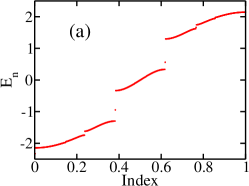
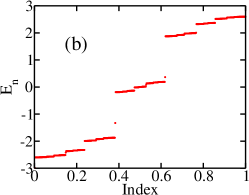
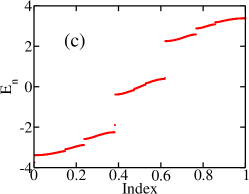
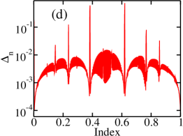
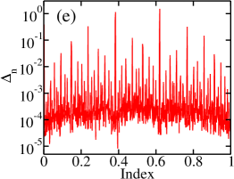
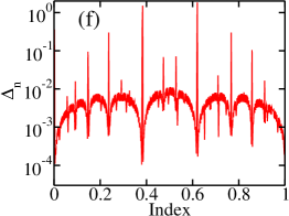
Figure 1: (a-c) Single particle energy spectra $E_{n}$ for $\lambda=1.0,2.0$, and $3.0$ respectively. (d-f) The corresponding level-spacing spectra $\Delta_{n}$ of the AAH model in logscale for $\lambda=1.0,2.0$ and $3.0$ respectively. For all plots $N=512$. Here index is the serial number of energy (gap) levels divided by the total number of energy (gap).

The Aubry-André-Harper (AAH) model in one dimension is given by the Hamiltonian Aubry and André (1980); Harper (1955):

$$H= -J\sum\limits_{i}^{N}(c_{i}^{\dagger}c_{i+1}+H.c.)$$ (1)

$$+\sum\limits_{i}^{N}\lambda\cos(2\pi\alpha i+\theta_{p})c_{i}^{\dagger}c_{i},$$

where $c_{i}^{\dagger}$ ($c_{i}$) represents the single particle creation (annihilation) operator at site $i$. We consider a lattice on a circular ring of total number of sites $N$. Here $\lambda$ is the strength of the quasi-periodic potential with quasi-periodicity $\alpha$, an irrational number and an arbitrary phase $\theta_{p}$. The strength of the nearest-neighbor hopping is $J$. When the irrational number $\alpha$ is chosen to be a Diophantine number, all the single particle eigenstates of the AAH model become delocalized for $\lambda<2J$ and localized for $\lambda>2J$, $\lambda=2J$ being the quantum critical point, where all the eigenstates are multifractal Modugno (2009). Also at $\lambda=2J$, the AAH model in position space maps to itself in the momentum space, thus making the model self-dual at $\lambda=2J$ Thouless (1983). In this work, we will assume $J=1$ and $\alpha=(\sqrt{5}-1)/2$, which is inverse of the golden mean, unless otherwise stated.

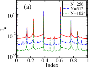
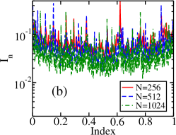
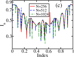
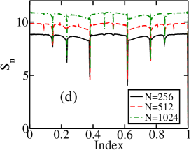
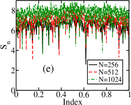
Figure 2: (a-c) IPR of all the single particle eigenstates in logscale for $\lambda=1.0,2.0$ and $3.0$ respectively. (d-f) von Neumann entropy $S_{n}$ of all the single particle eigenstates for $\lambda=1.0,2.0$ and $3.0$ respectively. In all the plots the dependence on system size $N$ is studied. Here index is the serial number of eigenstate divided by the total number $N$.

II.1 Generics of spectrum

The single particle energy spectrum $E_{n}$ and the nearest level spacing $\Delta_{n}=E_{n+1}-E_{n}$ of the AAH model have already been investigated in seminal works Tang and Kohmoto (1986); Evangelou and Pichard (2000); Takada et al. (2004); Machida and Fujita (1986). It can be mathematically shown that the energy spectrum forms a Cantor set-like self-similar structure Avila and Jitomirskaya (2009). The energy level-spacing distribution of the AAH model is not Wigner-like in the delocalized phase Evangelou and Pichard (2000) whereas it is Poissonian in the localized phase Machida and Fujita (1986); Takada et al. (2004). At the critical point, the level-spacing distribution satisfies an inverse power law Takada et al. (2004); Evangelou and Pichard (2000). The energy spectra and the corresponding level-spacing spectra for the delocalized, multifractal and localized phases are shown in Fig. 1. Due to the Cantor set structure of the spectra, there are many gaps between the subbands Fig. 1(a-c), whose specific locations, are related to the irrational number $\alpha$, to be discussed next. There are isolated states in the spectrum in the large gaps, represented by the isolated dots in 1(a). However, these isolated states vanish if one chooses system size $N$ to be a Fibonacci number, defined later in Equation 8.

II.2 Special locations of band gaps

In Figs. 1(a) and 1(d) the large gaps are apparent when the fractional index is $\approx\alpha,\alpha^{2},\alpha^{3},\alpha^{4}(\approx 0.618,0.382,0.236,0.145)$ etc. The fluctuations in the gap become maximum at the quantum critical or the multifractal point $\lambda=2$ (Fig. 1(e)) Evangelou and Pichard (2000) and the magnitude of the gaps increases as $\lambda$ increases(Fig. 1(f)). In this work, we explore the effect of such gaps on the transport properties at the single and many particle levels, especially in the delocalized phase. Also the localization properties of the single-particle eigenstates near the locations of these band gaps may be very different from the other eigenstates, which we will explore in the next section.

III Single-particle transport properties

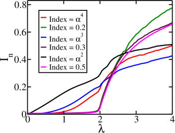
Figure 3: Variation of IPR with $\lambda$ of the single particle eigenstates near the locations of the large band gaps (Index $\approx\alpha^{4},\alpha^{3},\alpha^{2}$) compared to the other eigenstates (with Index $=0.2,0.3,0.5$ )respectively. For all the plots $N=256$. To smooth out the curve, an average over $100$ values of $\theta_{p}$ (running from $0$ to $2\pi$ in uniform steps) is performed.

In order to study the transport properties of a single particle in AAH potential, we have analyzed the inverse participation ratio (IPR) and the von Neumann entropy. For simplicity all the results presented in this section are calculated assuming $\theta_{p}=0$ unless mentioned. We briefly review these quantities and present our results in the following.

III.1 Inverse participation ratio

The inverse participation ratio (IPR) is a key quantity for studying delocalization-localization transitions, which is defined as:

$$I_{n}=\sum_{i=1}^{N}|\psi_{n}(i)|^{4},$$ (2)

where the $n\textsuperscript{th}$ normalized single-particle eigenstate $\ket{\psi_{n}}=\sum_{i=1}^{N}\psi_{n}(i)\ket{i}$ is written in terms of the Wannier basis $\ket{i}$, representing the state of a single particle localized at the site $i$ of the lattice. For a perfectly delocalized eigenstate $I_{n}=1/N$ whereas $I_{n}=1$ for a single-site localized eigenstate. In the critical phases $I_{n}$ is expected to show an intermediate behavior. In Fig. 2(a-c) the IPR for all the eigenstates can be seen for $\lambda=1$(delocalized), $\lambda=2.0$(multifractal) and $\lambda=3.0$(localized) respectively. The IPR shows sudden jumps exactly where the sub-band gaps can be found as can be seen from Fig. 2(a). In the delocalized phase typically IPR$\sim 1/N$ except at these special points where IPR behaves anomalously with $N$. At the multifractal point, the fluctuations become maximum and the IPR shows anomalous scaling with $N$ almost all over the spectrum 2(b). In the localized phase, the IPR overlap with each other for different values of $N$ 2(c). However, in this phase one obtains dips, instead of peaks, at the positions of large band gaps.

III.2 von Neumann entropy

It is now well established that entanglement entropy is a good measure to explore localization phenomena in quantum systems . In this work we aim to calculate von Neumann entropy connected to a single-site. As a single particle has two local states $\ket{0}_{i}$ and $\ket{1}_{i}$ at the site $i$, the local density matrix $\rho_{n,i}$ for the $n\textsuperscript{th}$ eigenstate can be written as Jia et al. (2008):

$$\rho_{n,i}=|\psi_{n}(i)|^{2}\ket{1}_{i}\bra{1}_{i}+(1-|\psi_{n}(i)|^{2})\ket{0}_{i}\bra{0}_{i}.$$ (3)

The von Neumann entropy associated with site $i$ is then given by Gong and Tong (2008):

$$S_{n,i}= -|\psi_{n}(i)|^{2}\log_{2}(|\psi_{n}(i)|^{2})$$ (4)

$$-(1-|\psi_{n}(i)|^{2})\log_{2}(1-|\psi_{n}(i)|^{2}).$$

In a delocalized eigenstate $|\psi_{n}(i)|^{2}=1/N$ and hence $S_{n,i}\approx\frac{1}{N}\log_{2}N+\frac{1}{N}$ for large value of $N$ whereas for a single-site localized state $S_{n,i}=0$. The contributions from all sites for a single-particle eigenstate are given by:

$$S_{n}=\sum_{i=1}^{N}S_{n,i}.$$ (5)

For large values of $N$, $S_{n}\approx(\log_{2}N+1)$ in the delocalized phase whereas $S_{n}\approx 0$ in the extremely (single-site) localized phase. For the critcal phases $S_{n}$ can take any intermediate values. As we can see from Fig. 2(a) the single particle von Neumann entropy $S_{n}$ has higher value in the delocalized phase and varies as $\log N$ but it shows sudden fall at the special points where IPR shows jumps and anomalous dependence on $N$. In the localized phase, as expected $S_{n}$ takes smaller values and shows no dependence on $N$ but instead of a sudden fall one obtains peaks at the special points [see Fig. 2(c)]. At the critical point, $S_{n}$ shows wide fluctuations and picks up intermediate values showing anomalous scaling with $N$, which is shown in Fig. 2(b).

To contrast the localization properties of the special eigenstates near the large band gaps with the non-special eigenstates, the $IPR$ is plotted as function of $\lambda$ in Fig. 3. As we can see from the figure, the non-special eigenstates undergo delocalization-localization transition at $\lambda=2$ as IPR changes abruptly, whereas the special eigenstates, with isolated energy levels, display different behaviour as IPR vs. $\lambda$ curves do not reflect criticality at $\lambda=2$. The contrasting localization properties of the special and non-special single particle eigenstates are consistent with the breakdown of the single-parameter scaling at the localization transition in quasiperiodic quantum systems, recently found in the literature Sutradhar et al. (2019). This kind of special feature of not reflecting the criticality of the model is present even in the behavior of the many-particle quantities when Fermi level is set in those band gaps. We discuss this in the following section. However, if one chooses the system size from the Fibonacci sequence such as $N=34,144,610$ (commensurate) as described in Eq. (8) of the paper, the isolated energy levels, as shown in Fig. 1(a), disappear and all the single particle eigenstates become delocalized for $\lambda<2$ and localized for $\lambda>2$. So the peaks in $I_{n}$ (and corresponding falls in $S_{n}$) as shown in Fig. 2(a) for $\lambda<2$ disappear. Also the distinction between the special states and non-special states in Fig. 3 vanishes in this case.

IV Many-particle transport properties

In this section, we consider non-interacting spinless fermions in the system. Since we have seen the surprising effect of energy gaps in the single-particle picture, we expect to see such effects even in the system of many fermions. We calculate many-fermionic entanglement entropy and persistent current and look at the behavior of these quantities as a function of the filling fraction $\nu=N_{p}/N$, where $N_{p}$ is the number of fermions in a periodic ring with $N$ sites. Entanglement entropy and persistent current have been studied very recently for the AAH model at half filling Roy and Sharma (2018); Roy and Sinha (2018). In what follows, we briefly describe the quantities and discuss our results.

IV.1 Entanglement entropy

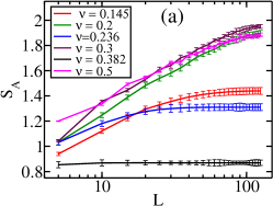
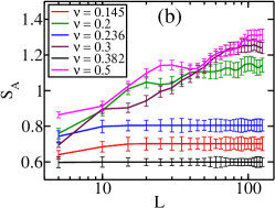
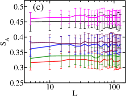
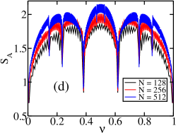
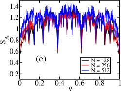
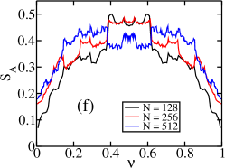
Figure 4: (a-c) Dependence of entanglement entropy $S_{A}$ of the many-body ground state on subsystem size $L$ (in logscale) for increasing values of the filling of fermions $\nu$ for $\lambda=1.0$(a), $\lambda=2.0$(b) and $\lambda=3.0$(c) respectively. For figures (a-c) $N=256$. (d-f) Variation of $S_{A}$ with $\nu$ for increasing system size $N$ for $\lambda=1.0$(d), $\lambda=2.0$(e) and $\lambda=3.0$(f) respectively. For the last three plots $L=N/2$. For all the plots, an average over $100$ values of $\theta_{p}$ (running from $0$ to $2\pi$ in uniform steps) has been carried out.

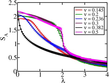
Figure 5: Variation of $S_{A}$ with $\lambda$ for increasing values of filling of fermions $\nu$. For all the plots $L=N/2$ where $N=256$ and an average over $100$ values for $\theta_{p}$ (running from $0$ to $2\pi$ in uniform steps) is carried out.

For pure states, von Neumann entropy has established itself as the standard measure of quantum entanglement, and has been extensively used to study different many-body phases and to make a distinction amongst them Eisert et al. (2010); Laflorencie (2016). Intuitively, one would expect that the greater the delocalization, the more the entanglement and vice versa, although exceptions exist Kannawadi et al. (2016). We start with a brief discussion of the calculation of the entanglement entropy of fermions in the ground statePeschel (2003); Peschel and Eisler (2009); Peschel (2012); Roy and Sharma (2018). For the fermionic many-body ground state $\Ket{\Psi_{0}}$, the density matrix can be written as $\rho=\Ket{\Psi_{0}}\Bra{\Psi_{0}}$. The entanglement entropy between two subsystems is then given by $S_{A}=-Tr(\rho_{A}\log\rho_{A})$, where the reduced density matrix is $\rho_{A}=Tr_{B}(\rho)$. However, for a single Slater determinant ground state, Wick’s theorem can be exploited to write the reduced density matrix as $\rho_{A}=\frac{e^{-H_{A}}}{Z}$, where $H_{A}=\sum\limits_{ij}H_{ij}^{A}c_{i}^{\dagger}c_{j}$ is called the entanglement Hamiltonian, and $Z$ is obtained from the condition $Tr(\rho_{A})=1$. The information contained in the reduced density matrix of size $2^{L}\times 2^{L}$ can be captured in terms of the correlation matrix $C$ of size $L\times L$Peschel (2003) within the subsystem $A$, where $C_{ij}=\left\langle c_{i}^{\dagger}c_{j}\right\rangle$. The correlation matrix and the entanglement Hamiltonian are related byPeschel (2003); Peschel and Eisler (2009); Peschel (2012):

$$C=\frac{1}{e^{H_{A}}+1}.$$ (6)

Using this relation, the entanglement entropy for free fermions is given byPeschel and Eisler (2009); Peschel (2012)

$$S_{A}=-\sum\limits_{m=1}^{L}[\zeta_{m}\log\zeta_{m}+(1-\zeta_{m})\log(1-\zeta_{m})],$$ (7)

where $\zeta_{m}$’s are the eigenvalues of the correlation matrix $C$. Subsystem scaling of entanglement entropy has been used to distinguish quantum phases Eisert et al. (2010); Laflorencie (2016); Roy et al. (2019). For free fermions in $d$ dimension, typically $S_{A}\propto L^{d-1}\log L$ Swingle (2010) in metallic phases and $S_{A}\propto L^{d-1}$ in the localized phase in the presence of disorder. To produce smoother $S_{A}$ vs. $L$ plots for the AAH model, we have done an average of $S_{A}$ over $100$ (non-random) values of $\theta_{p}\in[0,2\pi]$ in uniform steps. Scaling of $S_{A}$ of the many-fermionic ground state with $L$ is shown in Fig. 4(a),(b) and (c) for increasing values of $\nu$ for the delocalized, multifractal and localized phases respectively. As can be seen from Fig. 4(a), typically, in the delocalized phase $S_{A}\propto\log L$ including the half-filled case Roy and Sharma (2018) except when $\nu\approx\alpha^{2},\alpha^{3}$ and $\alpha^{4}(0.382,0.236$ and $0.145)$ where $S_{A}$ becomes a constant abiding by the area-law of entanglement entropy. In the localized phase, $S_{A}$ always follows area-law independent of $\nu$ 4(c). In the multifractal phase, generally $S_{A}$ scales in some intermediate manner with $L$ whereas the area-law persists when $\nu=0.145,0.236,0.382$. The variation of $S_{A}$ with $\nu$ is shown in Fig. 4(d-f) for increasing values of $N$ for $\lambda=1.0,2.0$ and $3.0$ respectively. In the delocalized phase, the sudden drops of $S_{A}$ at $\nu=0.145,0.236,0.382,0.618$ etc. are clearly visible in Fig. 4(d) coinciding with the appearance of large gaps in the energy spectrum. In the multifractal and localized phases, the energy spectrum becomes more fragmented due to appearance of large gaps. The fluctuations in $S_{A}$ maximize at the multifractal point and hence the $S_{A}$ vs. $\nu$ plots become more complicated [see Figs 4(e) and 4(f)]. However, the value of $S_{A}$ goes down as the strength of disorder $\lambda$ increases, which is shown explicitly in Fig. 5. It is to be noted that for the special values of $\nu={0.145,0.236,0.382}$ the criticality ($\lambda_{c}=2$) of the AAH model is not reflected in the behavior of $S_{A}$ with $\lambda$ whereas for other values of filling ($\nu={0.2,0.3,0.5}$) there is a sharp decrease of $S_{A}$ at $\lambda_{c}=2$ indicating the inherent critical nature of the model. It is to be noted that the results presented here on the entanglement entropy remains unaffected if one chooses to study with the system sizes which are Fibonacci numbers $N=34,144,610$ etc., unlike the single particle quantities discussed previously. This indicates that the many-particle phenomena are not governed by the presence or absence of the isolated single particle localized states in the large band gaps. Rather many-particle results are the manifestation of the large gaps in the single particle energy spectrum.

IV.2 Persistent current

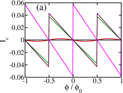
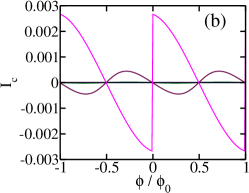
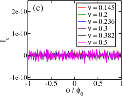
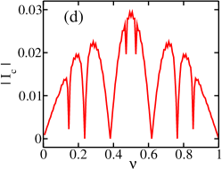
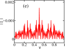
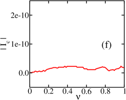
Figure 6: (a-c) Persistent current $I_{c}$ as function of the flux $\phi$ in unit of $\phi_{0}$ for increasing values of filling fraction $\nu$ for $\lambda=1.0,2.0$ and $3.0$ respectively. For all plots (a-c) different colors denote different values of $\nu$ as defined in (c). (d-f) $|I_{c}|$ as function of $\nu$ for $\lambda=1.0,2.0$ and $3.0$ respectively at fixed $\phi=0.25\phi_{0}$. For all the plots $\alpha=377/610$ with $N=610$.

Figure 7: The absolute value of the persistent current $|I_{c}|$ as function of $\lambda$ for increasing values of $\nu$ at fixed $\phi=0.25\phi_{0}$. For all the plots $\alpha=377/610$ with $N=610$.

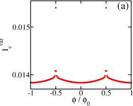
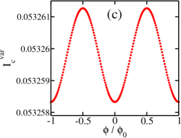
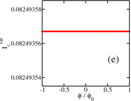
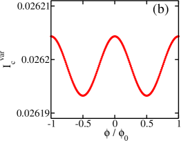
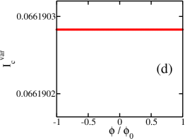
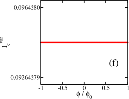
Figure 8: Dependence of the variance of persistent current $I_{c}^{var}$ on the flux $\phi$ (in units of $\phi_{0}$) for fermions with different filling fractions $\nu$ and for increasing values of the strength $\lambda$ of the quasiperiodic potential. Fig. (a), (c) and (e): $I_{c}^{var}$ vs $\phi$ plots for $\lambda=1.0,2.0$ and $3.0$ respectively and fixed regular value of $\nu=0.2$. Fig. (b), (d) and (f): $I_{c}^{var}$ vs $\phi$ plots for $\lambda=1.0,2.0$ and $3.0$ respectively and fixed special value of $\nu=0.236$. Total number of sites $N=144$ and $\alpha=89/144$ for all the plots.

Next we discuss the persistent current in the fermionic system, which has also been used to study localization phenomena Imry (2008). Persistent current can be generated by applying a phase twist at the boundary. With periodic boundary conditions this is equivalent to attaching a flux to the fermions moving in a ring. In a mesoscopic quantum ring a persistent current of electrons can be produced by applying a magnetic flux $\phi$ inside the ring. In a quantum ring the current-flux relationship can depend on factors such as band structure, disorder, interaction, ring geometry, number of particles etc. In this work, we mainly focus on the current-flux relationship and its variation with the strength of quasi-periodic disorder $\lambda$ of the AAH model and the filling fraction $\nu=N_{p}/N$ of the $N_{p}$ fermions in a ring of $N$ sites. We will put $\theta_{p}=0$ for all the results presented in this section. An irrational number can be expanded as a continued fraction Cohn (2006), which makes possible a successive rational approximation of it in the form of $a_{0}/b_{0}$, where $a_{0}$ and $b_{0}$ are coprime integers. A rational approximation of $\alpha$ is given by $\alpha=F_{s-1}/F_{s}$ for two successive members in the series defined as Falcon (2014):

$$F_{s}=F_{s-1}+F_{s-2}$$ (8)

with $F_{0}=0$, $F_{1}=1$, which converges to the inverse of the ‘golden mean’ $(\sqrt{5}-1)/2$ in the limit $s\rightarrow\infty$. We will make a rational approximation over $\alpha$ as described above along with $N=F_{s}$ to validate the periodic boundary condition in this section. In order to calculate the persistent current we consider a phase-twisted Hamiltonian for fermions, which is given by:

$$H(\theta)=-J\sum_{l}(e^{-i\theta/N}c_{l}^{\dagger}c_{l+1}+H.c.)+\lambda\sum\limits_{l}\cos(2\pi\alpha l)c_{l}^{\dagger}c_{l},$$

(9)

where $c_{l}$ is the fermionic annihilation operator acting on site $l$ and $\theta=2\pi\frac{\phi}{\phi_{0}}$, where $\phi_{0}=h/e$ is the unit flux quanta. After diagonalization of this Hamiltonian, the single particle energy levels $\epsilon_{n}(\phi)$ are used to calculate the persistent current Imry (2008); Cheung et al. (1988):

$$I_{c}(\phi)=-\frac{\partial E_{0}}{\partial\phi}$$ (10)

where $E_{0}=\sum_{n}\epsilon_{n}(\phi)\theta(E_{F}-\epsilon_{n})$ is the ground state energy of the system and $E_{F}$ is the Fermi energy at zero temperature. In the absence of any potential, the energy dispersion is given by $\epsilon_{n}(\phi)=-2J\cos(\frac{2\pi}{N}(n+\frac{\phi}{\phi_{0}}))$ where $-{N}/2\leq n<{N}/2$. For $N_{p}$ fermions in $N$ sites, the persistent current can be written asCheung et al. (1988):

$$I_{c}=-I_{0}\frac{\sin(\frac{\pi}{N}(2\frac{\phi}{{\phi}_{0}}+\eta))}{\sin(\frac{\pi}{N})},$$ (11)

where $I_{0}=\frac{4\pi J}{N{\phi}_{0}}\sin(N_{p}\pi/N)$. The persistent current $I_{c}$ exhibits periodic variation with flux $\phi/\phi_{0}$ and a phase shift $\eta$ is generated due to the parity of the number of fermions $N$. For odd $N_{p}$, $\eta=0$ in region $-0.5\leq\frac{\phi}{{\phi}_{0}}<0.5$ and for even $N_{p}$, $\eta=-1$ in region $0\leq\frac{\phi}{{\phi}_{0}}<1$. The persistent current decreases with system size as $I_{0}\propto 1/N$ and it is maximum when $\nu=0.5$ since $I_{0}$ is maximum at the same point.

Now as the AAH disorder is turned on, the current-flux plots are shown in Fig. 6. In the delocalized phase, $I_{c}$ is almost vanishing for all values of $\phi$ when $\nu=0.145,0.236,0.382$. Otherwise the maximum of $I_{c}$ increases with $\nu$ [Fig. 6(a))]. The $I_{c}-\phi$ plots look like sawtooth curves because when $N$ is very large, one can use in Eq. 11, the small-angle approximation for the sine function: $(\sin(x)\approx x)$. In the critical phase $I_{c}$ is periodic with $\phi$ but its magnitude is very small whereas $I_{c}$ is still vanishing for special values of $\nu$ as mentioned before [Fig. 6(b)]. In the localized phase $I_{c}$ vanishes for all values of $\phi$ and $\nu$ [Fig. 6(c))] as has been reported for the particular case of half-filling Roy and Sinha (2018). The absolute value of the persistent current $|I_{c}|$ as function of $\nu$ for three values of $\lambda=1.0,2.0,3.0$ at fixed value of $\phi=0.25\phi_{0}$ is plotted in Figs. 6(d)-6(f). The current falls off substantially at the special filling $\nu=0.145,0.236,382$ even when the system is in the delocalized phase in Fig. 6(d) similar to the dependence of $S_{A}$ on $\nu$ as shown in Fig. 4(d). In the multifractal phase, the magnitude of current significantly decreases whereas its fluctuations increase as function of $\nu$ as shown in Fig. 6(e) similar to $S_{A}$ in multifractal phase [Fig. 4(e)]. The current vanishes for all values of $\nu$ as one goes into the localized phase as can be seen from Fig. 6(f). The dependence of $|I_{c}|$ on $\lambda$ for increasing values of $\nu$ at fixed $\phi$ is shown in Fig. 7. The criticality of the AAH model is evident from the $I_{c}-\lambda$ plots for normal filling $\nu=0.2,0.3,0.5$ as $I_{c}$ vanishes at $\lambda_{c}=2$ for those fillings whereas $I_{c}$ goes to zero for smaller values of $\lambda<2$ well before $\lambda=2$ for non-trivial $\nu=0.145,0.236,0.382$. This shows that the critical nature of the model is somehow suppressed at those fillings as is also clear from Fig. 5.

The persistent current can also be calculated from the expectation value of the current operator defined as $J^{c}=-\frac{\partial H}{\partial\phi}$. The current operator can thus be written as:

$$J^{c}=\sum_{l}J^{c}_{l,l+1}$$ (12)

where $J^{c}_{l,l+1}=-i\frac{2\pi J}{N}(e^{-i\frac{2\pi\phi}{\phi_{0}N}}c_{l}^{\dagger}c_{l+1}-e^{i\frac{2\pi\phi}{\phi_{0}N}}c_{l+1}^{\dagger}c_{l})$ and $\phi$ is expressed in the units of $\phi_{0}$. The two definitions of the persistent current are related via the Feynman-Hellmann (FH) theorem as $\langle-\frac{\partial H}{\partial\phi}\rangle=-\frac{\partial E_{0}}{\partial\phi}$, except at points of degeneracies Zhang and George (2002); Alon and Cederbaum (2003); Fernández (2004); Vatsya (2004) in the energy spectrum. At the degenerate points, the system has many eigenfunctions corresponding to a single energy and any linear combination of the true eigenfunctions also satisfies the Schrödinger equation. As FH theorem equates two quantities involving eigenfunctions and eigenvalues respectively, the equality apparently becomes invalid in the presence of degeneracies in the eigenvalues (for details, see Appendix A).

IV.3 Variance of persistent current

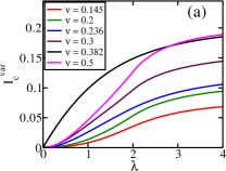
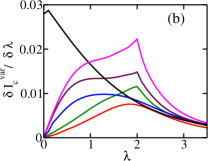
Figure 9: (a) The variation of $I_{c}^{var}$ with $\lambda$ for the fixed $\phi=0.25\phi_{0}$ for regular and special filling fractions $\nu$ of fermions. (b) The first derivative of $I_{c}^{var}$ with $\lambda$ for the fixed $\phi=0.25\phi_{0}$ for increasing filling fractions $\nu$ of fermions. Total number of sites $N=144$ and $\alpha=89/144$ for all the plots.

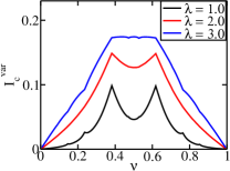
Figure 10: Dependence of the variance of persistent current $I_{c}^{var}$ on the filling fraction $\nu$ for increasing values of the strength $\lambda$ of the quasiperiodic potential and fixed $\phi=0.25\phi_{0}$. Total number of sites $N=144$ and $\alpha=89/144$ for all the plots.

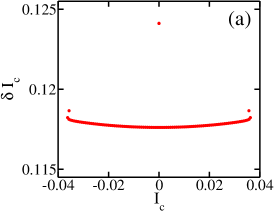
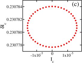
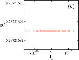
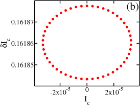
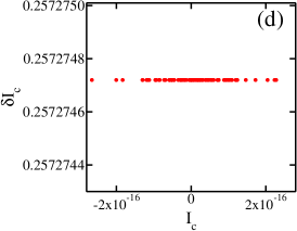
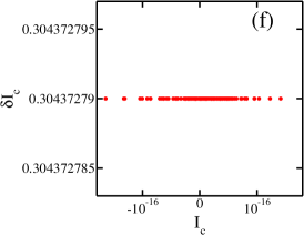
Figure 11: The $\delta I_{c}$-$I_{c}$ curves for fermions with different filling fractions $\nu$ and for increasing values of the strength $\lambda$ of the quasiperiodic potential. Fig. (a), (c) and (e): $\delta I_{c}$-$I_{c}$ curves for $\lambda=1.0,2.0$ and $3.0$ respectively and fixed regular value of $\nu=0.2$ Fig. (b), (d) and (f): $\delta I_{c}$-$I_{c}$ curves for $\lambda=1.0,2.0$ and $3.0$ respectively and fixed special value of $\nu=0.236$. Total number of sites $N=144$ and $\alpha=89/144$ for all the plots.

A study of the fluctuations of observables in quantum systems can be very profitable, as they carry important information about the systems, sometimes more than the mean values of the observables. Here we will study the persistent current, computed using the definition $I_{c}=\langle J^{c}\rangle$, as described in Eq. 12. The variance of the persistent current is given by:

$$I_{c}^{var}=\langle{J^{c}}^{2}\rangle-\langle{J^{c}}\rangle^{2},$$ (13)

where

$${J^{c}}^{2}=\sum_{l}{J^{c}_{l,l+1}}^{2}+\sum_{l\neq l^{\prime}}J^{c}_{l,l+1}J^{c}_{l^{\prime},l^{\prime}+1}$$

, (14)

and

$$\langle{J^{c}_{l,l+1}}^{2}\rangle= -{\frac{4\pi^{2}J^{2}}{N^{2}}}(2\langle c_{l}^{\dagger}c_{l}\rangle\langle c_{l+1}^{\dagger}c_{l+1}\rangle$$

$$-2\langle c_{l}^{\dagger}c_{l+1}\rangle\langle c_{l+1}^{\dagger}c_{l}\rangle-\langle c_{l+1}^{\dagger}c_{l+1}\rangle-\langle c_{l}^{\dagger}c_{l}\rangle),$$

$$\langle J^{c}_{l,l+1}J^{c}_{l^{\prime},l^{\prime}+1} +J^{c}_{l^{\prime},l^{\prime}+1}J^{c}_{l,l+1}\rangle=-{\frac{4\pi^{2}J^{2}}{N^{2}}}[(\langle c_{l}^{\dagger}c_{l^{\prime}+1}\rangle\delta_{l^{\prime},l+1}$$ (15)

$$+2\langle c_{l}^{\dagger}c_{l+1}\rangle\langle c_{l\prime}^{\dagger}c_{l^{\prime}+1}\rangle-2\langle c_{l}^{\dagger}c_{l^{\prime}+1}\rangle\langle c_{l^{\prime}}^{\dagger}c_{l+1}\rangle)e^{-i2\theta}$$

$$-(2\langle c_{l}^{\dagger}c_{l+1}\rangle\langle c_{l^{\prime}+1}^{\dagger}c_{l^{\prime}}\rangle-2\langle c_{l}^{\dagger}c_{l^{\prime}}\rangle\langle c_{l^{\prime}+1}^{\dagger}c_{l+1}\rangle)]$$

$$+h.c.$$

The variation of $I_{c}^{var}$ with $\phi$ is shown in Fig. 8 for regular filling $\nu=0.2$ and special filling $\nu=0.236$ in the delocalized $(\lambda=1.0)$, critical $(\lambda=2.0)$ and localized $(\lambda=3.0)$ phases respectively. The variance of current varies periodically with flux but it becomes discontinuous if the Fermi level overlaps with quasi-degenerate levels $(\phi=\pm 0.5\phi_{0})$ for regular fillings ($\nu=0.2$ in the figure) in the delocalized phase $\lambda<2$ as can be seen from Fig. 8(a). However, for special fillings ($\nu=0.236$ in Fig. 8(b)) $I_{c}^{var}$ shows a continuous sinusoidal variation with $\phi$ as the Fermi level does not lie within degenerate levels for any value of $\phi$. At the critical point $\lambda=2.0$, $I_{c}^{var}$ vs. $\phi$ plots become sinusoidal for regular fillings due to lifting of the degeneracies as shown in Fig. 8(c) for $\nu=0.2$ whereas $I_{c}^{var}$ becomes independent of $\phi$ for special fillings (see Fig. 8(d)). In the localized phase $I_{c}^{var}$ is constant for both types of fillings as shown in Fig. 8(e) and Fig. 8(f) respectively. For clarity, a fixed value of $\phi=0.25\phi_{0}$ is chosen for which the Fermi level is always non-degenerate for any filling fraction $\nu$. For $\phi=0.25\phi_{0}$ the variation of $I_{c}^{var}$ with $\lambda$ is shown for regular and special values of $\nu$ in Fig. 9(a). The variance of current monotonically increases with $\lambda$ as the fluctuations of quantum observables increase with localization. The first derivative of $I_{c}^{var}$ with respect to $\lambda$ is calculated as a function of $\lambda$ to show how the slope of the plots in Fig. 9(a) change across the delocalization-localization transition. It turns out that for the regular fillings, the change of slope shows a maximum at the transition point $\lambda=2$ whereas no such peaks appear at the same point in the plots for special fillings [see Fig. 9(b)]. The variation of $I_{c}^{var}$ with filling fraction $\nu$ is shown in Fig. 10 for $\lambda=1.0,2.0$ and $3.0$ respectively. In the delocalized phase ($\lambda=1.0$), the plot shows sudden increase of $I_{c}^{var}$ at the values of special fillings whereas those maxima disappear as one gets into the localized phase. Such increase of quantum fluctuations is a property of localized systems which indicates that the fermionic system behaves like a localized one for special fillings even when $\lambda<2$.

IV.4 Relation between persistent current and its fluctuations

In this subsection, we will explore the relationship between the persistent current $I_{c}$ and its standard deviation $\delta I_{c}$, which are related by,

$$\delta I_{c}=\sqrt{I_{c}^{var}}$$ (16)

The $\delta I_{c}$ vs. $I_{c}$ plots are shown in Fig. 11. These plots are obtained by varying the flux uniformly in the entire range $\phi\in[-\pi\phi_{0},\pi\phi_{0}]$. In the delocalized phase, the $\delta I_{c}$-$I_{c}$ curves are open and discontinuous for the non-special values of $\nu$ due to the presence of quasi-degeneracies in the energy spectrum, as shown in Fig. 11(a) whereas these are closed continuous curves for the special fillings as can be seen from Fig. 11(b) due to no degeneracies. Such discontinuous $\delta I_{c}$-$I_{c}$ curves at the degenerate points have been recently reported for a one-dimensional model without any disorder Metcalf et al. (2018). At the critical phase, the $\delta I_{c}$-$I_{c}$ curves are closed ones for the non-special $\nu$ due to the lifting of degeneracies [Fig. 11(c)] and the curves are straight lines for special values of $\nu$ [Fig. 11(d)]. In the localized phase, the $\delta I_{c}$-$I_{c}$ curves are horizontal lines for any value of $\nu$ [see Figs. 11(e) and 11(f)]. The area enclosed by the $\delta I_{c}$-$I_{c}$ curves can be calculated to distinguish between the non-special and special fillings across the delocalization-localization transition in the AAH model. For the non-special values of $\nu$, the area is undefined in the delocalized phase for $\lambda<2$ due to quasi-degeneracies at the specific values of $\phi$. At $\lambda=2$, for the non-special values of $\nu$, the $\delta I_{c}$-$I_{c}$ curves are closed ones and the area enclosed by these are finite whereas the area goes to zero in the localized phase $\lambda>2$ as shown in Fig.12(a). For the special fillings, for small values of $\lambda$ the area is finite but it goes to zero as $\lambda$ increases well before it reaches the critical point $\lambda=2$ as can be seen in Fig. 12(b). This once again reinforces the finding that the criticality of the AAH model is reflected by the non-special fillings but not by the special fillings.

It is noteworthy that although the isolated single particle localized states are absent in single-particle spetra when the system size is chosen to be a Fibonacci number ($N=144,610,...$), the many-particle results on the persistent current depend on whether the values of filling fraction $\nu$ are special ones or not. Hence, this establishes that the contrasting behavior between the two kinds of filling fractions is a manifestation of the large gaps in the single-particle spectra rather than the presence or absence of the isolated localized single particle states. We would like to mention that there are large gaps above the Fermi level when $\nu=\alpha,\alpha^{2},\alpha^{3},\alpha^{4}$, which approximately evaluates to $\nu=0.618,0.382,0.236,0.145$. One has to choose the numerical values of $\alpha$ carefully so that there is a large gap above the Fermi level. The results remain qualitatively unchanged even for smaller system sizes. However, the delocalization-localization transition at $\lambda=2$ for non-special filling fractions becomes sharper as the system size $N$ increases. For special filling fractions the system gets localized at $\lambda<2$. As system size increases, these localization transition points shift to lower values of $\lambda$. Hence quantitatively, the distinctions between special fillings and non-special fillings as shown in Fig.5, Fig.7, Fig.9, Fig.12 etc. become sharper as one goes from smaller to larger system sizes.

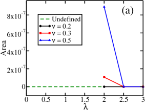
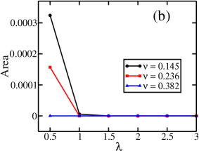
Figure 12: (a) The area enclosed by the $\delta I_{c}$-$I_{c}$ curves as function of $\lambda$ for non-special filling fractions. The green dotted line represents region where area connot be defined as a closed curve is not obtained due to quasi-degeneracies. (b) The area enclosed by the $\delta I_{c}$-$I_{c}$ curves as function of $\lambda$ for special filling fractions. For all the plots $N=144$ and $\alpha=89/144$. The $\delta I_{c}$-$I_{c}$ curves are plotted by varying $\phi\in[-\pi,\pi]\phi_{0}$.

V Conclusion

We have studied the effect of the single particle energy gaps on the transport properties (single-particle and many-particle fermionic) of the AAH potential in one dimension. Even in the well known delocalized phase ($\lambda<2$), the IPR and von Neumann entropy of the single-particle eigenstates drastically rise and fall off respectively for non-Fibonacci system sizes when the eigenstate index $=\alpha,\alpha^{2},\alpha^{3},\alpha^{4}(\approx 0.618,0.382,0.236,0.145)$. The single particle spectrum contains large gaps above the energy levels with these special indices. The eigenstates with the special indices are isolated states with a different kind of localization properties as compared to the other eigenstates. However, these isolated localized states disappear when the system sizes are Fibonacci numbers such as $N=144,610$ etc. For Fibonacci system sizes, all the single particle eigenstates have the same kind of localization properties and the peaks (falls) in the IPR (von Neumann entropy) vanish.

Next we have considered the many-particle properties of the free fermionic ground states. The entanglement entropy falls off substantially when the filling fraction is $\nu=\alpha^{2},\alpha^{3},\alpha^{4}(\approx 0.382,0.236,0.145)$. Also the subsystem scaling of $S_{A}$ follows the area-law at the same special values of $\nu$ whereas in the delocalized phase $S_{A}$ shows logarithmic violation of the area-law for normal fillings $\nu=0.2,0.3,0.5$. The entanglement entropy of the fermionic ground states with special values of $\nu$ do not seem to show any signatures of criticality at $\lambda_{c}=2$ unlike the non-special fillings. All these filling-dependent features on many-particle entanglement entropy are completely independent of whether or not the system size is a Fibonacci number. This proves that the contrasting behavior of the entanglement entropy for the special and non-special fillings is a manifestation of the large gaps rather than the isolated localized states in the single particle spectra. The persistent current of fermions exhibits similar striking filling-fraction dependent behavior. It is vanishingly small even in the delocalized phase for those special fillings and the criticality of the AAH model is not reflected in the behavior of the current with $\lambda$. We have also calculated the variance of the persistent current and explored its relations with the mean value of persistent current in our model. In the delocalized phase, the standard deviation vs. mean persistent current curves are discontinuous for the non-special values of filling fractions and continuous (closed) for the special values of filling fractions whereas these curves become straight lines in the localized phase for both types of filling fractions. The area enclosed by these curves can be used to distinguish between the non-special filling fractions and special filling fractions across the delocalization-localization transition. In the delocalized phase, the area is undefined for non-special fillings and finite for special fillings whereas the area is zero in the localized phase for all fillings.

The persistent current depends on whether the values of filling fraction are special ones or not even when system sizes are Fibonacci numbers when the isolated single particle localized states are absent in the single particle spectra. Hence, this again establishes that the interesting many particle phenomena depend on the locations of large gaps in the single particle energy spectra rather than on the presence or absence of the isolated localized states. The effect of energy gap structures on transport properties as described in this work has been hitherto unexplored. The connection between the persistent current and its quantum fluctuations is very interesting and may be extended to other contexts like the many-body localization. The filling fraction dependent persistent current is one of the striking aspects of our work. This may potentially be tested in cold atom based experiments Ryu et al. (2007); Eckel et al. (2014); Goldman et al. (2014); Chien et al. (2015) by creating a synthetic flux in bichromatic optical lattices, given that the results are independent of system sizes and even valid for small system sizes. The non-equilibrium dynamics of a wave-packet with specific energy may be used to probe the single-particle transport properties as it has been done in Ref. Skipetrov and Sinha, 2018. A similar non-equilibrium study of a cleverly defined many-particle wave-packet may be useful in this regard, although this work is based on the equilibrium transport properties. Our results open up the possibility of further exploration of non-trivial filling-fraction dependent localization or delocalization phenomena in the AAH model. Hopefully our work will encourage the community to revisit the energy spectra of quantum systems with quasi-periodic potential and thus help fine-tune our understanding of filling-fraction dependence.

Appendix A Degeneracy and persistent current: no disorder case

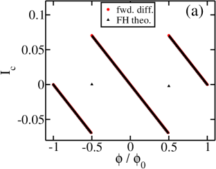
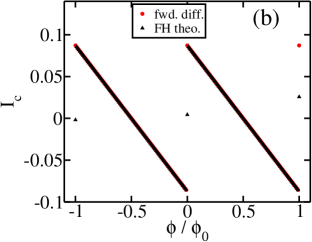
Figure 13: Comparison of two approaches to compute the persistent current. (a) The variation of persistent current $I_{c}$ with the flux $\phi$ (in units of $\phi_{0}$) for fermions with filling fraction $\nu=0.3$ calculated by taking derivative of the ground state energy using “forward difference” method and by taking the expectation of the current operator, which is connected to the first method via ‘FH’ theorem. (b) The same plot for $\nu=0.5$. Total number of sites $N=144$ and disorder strength $\lambda=0$ for all the plots.

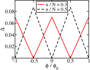
Figure 14: Dependence of the single particle gaps $\Delta$ on the flux $\phi$ (in units of $\phi_{0}$) at the $n\textsuperscript{th}$ energy level where $n/N=0.3$ and $0.5$ respectively. Total number of sites $N=144$ and disorder strength $\lambda=0$ for all the plots.

In this appendix we will discuss breakdown of the Feynman-Hellmann (FH) theorem in presence of degeneracies and how that shows up in the calculation of the persistent current and its variance for a one-dimensional tight binding chain without any disorder. According to FH theorem

$$\langle-\frac{\partial H}{\partial\phi}\rangle=-\frac{\partial E_{0}}{\partial\phi},$$ (17)

which simplifies to

$$\langle J^{c}\rangle=-\frac{\partial E_{0}}{\partial\phi},$$ (18)

where $E_{0}$ is energy of the many-fermionic ground state, flux $\phi$ (in units of $\phi_{0}$) and $J^{c}$ is defined in the main text Eq. 12, which is calculated using the elements of the correlation matrix. So the left-hand side of Eq. 18 involves the fermionic ground state wavefunction whereas the right-hand side of the same involves the ground state energy. The single-particle energy dispersion for a one-dimensional periodic lattice without any disorder is given by,

$$\epsilon_{n}=-2J\cos\bigg{(}\frac{2\pi}{N}\bigg{(}n+\frac{\phi}{\phi_{0}}\bigg{)}\bigg{)},$$ (19)

where $n=0,\pm 1,\pm 2,\pm 3,...$. For a non-degenerate spectra, using $E_{0}=\sum_{n}\epsilon_{n}(\phi)\theta(E_{F}-\epsilon_{n})$ one obtains the expression of the persistent current written in Eq. 11 in the main text, using both the approaches depicted in Eq. 18. Figs. 13(a) and 13(b) show the variation of the persistent current $I_{c}$ with flux $\phi$ for filling fraction $\nu=0.3$ and $0.5$ respectively, computed using both the approaches for comparison. It is to be noted that there is an exact overlap between two methods except at $\phi=\pm 0.5\phi_{0}$ and $\phi=0,\pm 1\phi_{0}$ in Figs. 13(a) and 13(b) respectively. The $I_{c}-\phi$ curves look different for different fillings as number of fermions is odd in one case and even in the other case and as $I_{c}$ depends on whether the number of fermions is odd or even. When the Fermi level lies in the degenerate levels, the current by taking the derivative of the ground state energy calculated using the forward difference method happens to give the known exact results whereas the calculation of expectation of the current operator involving the ground state wavefunction gives a different result. The single-partcle energy gap $\Delta$ at the $n\textsuperscript{th}$ level is shown as function of flux $\phi$ for $n/N=0.3$ and $0.5$ respectively in Fig. 14. The gap vanishes at $\phi=\pm 0.5\phi_{0}$ and $\phi=0,\pm\phi_{0}$ respectively.

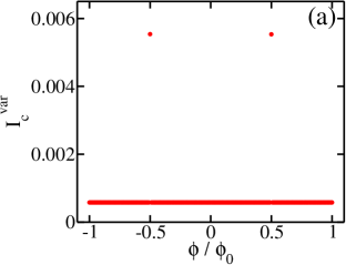
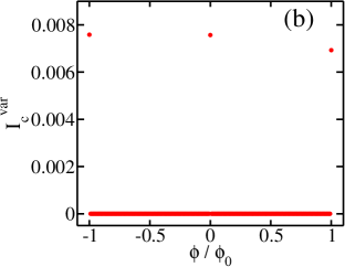
Figure 15: (a) The variation of $I_{c}^{var}$ with the flux $\phi$ (in units of $\phi_{0}$) for fermions with filling fraction $\nu=0.3$ calculated using Eq. 15. (b) The same plot for $\nu=0.5$. Total number of sites $N=144$ and disorder strength $\lambda=0$ for all the plots.

The variance of the persistent current $I_{c}^{var}$ as function of flux $\phi$ is shown in Fig. 15(a) and Fig. 15(b) for filling fractions $\nu=0.3$ and $0.5$ respectively. The curves show discontinuities exactly at the point of degeneracies as mentioned earlier. At the point of degeneracies, any linear superposition $\ket{\Psi_{0}}$ of the true ground states $\ket{\Phi_{0}}$ is also a valid solution of the Schr$\ddot{o}$dinger equation. On numerical computation, one does not obtain the true degenerate ground state and the FH theorem as mentioned in Eq. 18 breaks down in presence of degeneracies Zhang and George (2002); Alon and Cederbaum (2003); Fernández (2004); Vatsya (2004). The corrected FH theorem for degenerate case can be described by adding one additional condition in the degenerate subspace, written as Fernández (2004); Alon and Cederbaum (2003); Vatsya (2004)

$$\bra{\Phi_{0,i}}-\frac{\partial H}{\partial\phi}\ket{\Phi_{0,j}}=0\hskip 7.11317pt\text{for}\hskip 7.11317pti\neq j$$

$$\bra{\Phi_{0,i}}-\frac{\partial H}{\partial\phi}\ket{\Phi_{0,i}}=-\frac{\partial E_{0}}{\partial\phi}$$ (20)

where $i,j=1,...,q$ for the q-degenerate subspace. After numerically computing the ground states $\ket{\Psi_{0}}$’s at the degenerate point, one essentialy constructs matrix A given by

$$A_{ij}=\bra{\Psi_{0,i}}-\frac{\partial H}{\partial\phi}\ket{\Psi_{0,j}},$$ (21)

which contains off-diagonal elements. Then one diagonalizes the matrix A to obtain the correct linear superposition

$$\ket{\Phi_{0,i}}=\sum\limits_{j=1}^{q}C_{ij}\ket{\Psi_{0,j}}$$ (22)

that satisfies the conditions shown in Eq. 20. The degenerate points should be treated specially under the treatment charted out here. These details are included in the interest of completion, although we have not used such treatments in our work.

References

- Goldman and Kelton (1993) A. I. Goldman and R. F. Kelton, Rev. Mod. Phys. 65, 213 (1993).
- Kohmoto et al. (1987) M. Kohmoto, B. Sutherland, and C. Tang, Phys. Rev. B 35, 1020 (1987).
- Maciá (2005) E. Maciá, Reports on Progress in Physics 69, 397 (2005).
- Anderson (1958) P. W. Anderson, Phys. Rev. 109, 1492 (1958).
- Aubry and André (1980) S. Aubry and G. André, Ann. Israel Phys. Soc 3, 18 (1980).
- Harper (1955) P. G. Harper, Proc. Phys. Soc. A 68, 874 (1955).
- Kohmoto (1983) M. Kohmoto, Phys. Rev. Lett. 51, 1198 (1983).
- Hofstadter (1976) D. R. Hofstadter, Phys. Rev. B 14, 2239 (1976).
- Evangelou and Pichard (2000) S. N. Evangelou and J.-L. Pichard, Phys. Rev. Lett. 84, 1643 (2000).
- Tang and Kohmoto (1986) C. Tang and M. Kohmoto, Phys. Rev. B 34, 2041 (1986).
- Modugno (2009) M. Modugno, New Journal of Physics 11, 033023 (2009).
- Roy and Sinha (2018) N. Roy and S. Sinha, Journal of Statistical Mechanics: Theory and Experiment 2018, 053106 (2018).
- Roósz et al. (2014) G. m. H. Roósz, U. Divakaran, H. Rieger, and F. Iglói, Phys. Rev. B 90, 184202 (2014).
- Lahini et al. (2009) Y. Lahini, R. Pugatch, F. Pozzi, M. Sorel, R. Morandotti, N. Davidson, and Y. Silberberg, Phys. Rev. Lett. 103, 013901 (2009).
- Purkayastha et al. (2018) A. Purkayastha, S. Sanyal, A. Dhar, and M. Kulkarni, Phys. Rev. B 97, 174206 (2018).
- Eisert et al. (2010) J. Eisert, M. Cramer, and M. B. Plenio, Rev. Mod. Phys. 82, 277 (2010).
- Laflorencie (2016) N. Laflorencie, Physics Reports 646, 1 (2016), quantum entanglement in condensed matter systems.
- Alet and Laflorencie (2018) F. Alet and N. Laflorencie, Comptes Rendus Physique 19, 498 (2018), quantum simulation / Simulation quantique.
- Sharma and Rabani (2015) A. Sharma and E. Rabani, Phys. Rev. B 91, 085121 (2015).
- Nehra et al. (2018) R. Nehra, D. S. Bhakuni, S. Gangadharaiah, and A. Sharma, Phys. Rev. B 98, 045120 (2018).
- Bhakuni and Sharma (2018) D. S. Bhakuni and A. Sharma, Phys. Rev. B 98, 045408 (2018).
- Skipetrov and Sinha (2018) S. E. Skipetrov and A. Sinha, Phys. Rev. B 97, 104202 (2018).
- Froufe-Pérez et al. (2017) L. S. Froufe-Pérez, M. Engel, J. J. Sáenz, and F. Scheffold, Proceedings of the National Academy of Sciences 114, 9570 (2017), https://www.pnas.org/content/114/36/9570.full.pdf .
- Metcalf et al. (2018) M. Metcalf, C.-Y. Lai, M. Di Ventra, and C.-C. Chien, Phys. Rev. A 98, 053601 (2018).
- Thouless (1983) D. J. Thouless, Phys. Rev. B 28, 4272 (1983).
- Takada et al. (2004) Y. Takada, K. Ino, and M. Yamanaka, Phys. Rev. E 70, 066203 (2004).
- Machida and Fujita (1986) K. Machida and M. Fujita, Phys. Rev. B 34, 7367 (1986).
- Avila and Jitomirskaya (2009) A. Avila and S. Jitomirskaya, Annals of Mathematics 170, 303 (2009).
- Jia et al. (2008) X. Jia, A. R. Subramaniam, I. A. Gruzberg, and S. Chakravarty, Phys. Rev. B 77, 014208 (2008).
- Gong and Tong (2008) L. Gong and P. Tong, Phys. Rev. B 78, 115114 (2008).
- Sutradhar et al. (2019) J. Sutradhar, S. Mukerjee, R. Pandit, and S. Banerjee, Phys. Rev. B 99, 224204 (2019).
- Roy and Sharma (2018) N. Roy and A. Sharma, Phys. Rev. B 97, 125116 (2018).
- Kannawadi et al. (2016) A. Kannawadi, A. Sharma, and A. Lakshminarayan, EPL (Europhysics Letters) 115, 57005 (2016).
- Peschel (2003) I. Peschel, Journal of Physics A: Mathematical and General 36, L205 (2003).
- Peschel and Eisler (2009) I. Peschel and V. Eisler, Journal of Physics A: Mathematical and Theoretical 42, 504003 (2009).
- Peschel (2012) I. Peschel, Brazilian Journal of Physics 42, 267 (2012).
- Roy et al. (2019) N. Roy, A. Sharma, and R. Mukherjee, Phys. Rev. A 99, 052342 (2019).
- Swingle (2010) B. Swingle, Phys. Rev. Lett. 105, 050502 (2010).
- Imry (2008) Y. Imry, Introduction to mesoscopic physics, 2nd ed. (Oxford university press, 2008).
- Cohn (2006) H. Cohn, The American Mathematical Monthly 113, 57 (2006), https://doi.org/10.1080/00029890.2006.11920278 .
- Falcon (2014) S. Falcon, Applied Mathematics 5, 2226 (2014).
- Cheung et al. (1988) H.-F. Cheung, Y. Gefen, E. K. Riedel, and W.-H. Shih, Phys. Rev. B 37, 6050 (1988).
- Zhang and George (2002) G. P. Zhang and T. F. George, Phys. Rev. B 66, 033110 (2002).
- Alon and Cederbaum (2003) O. E. Alon and L. S. Cederbaum, Phys. Rev. B 68, 033105 (2003).
- Fernández (2004) F. M. Fernández, Phys. Rev. B 69, 037101 (2004).
- Vatsya (2004) S. R. Vatsya, Phys. Rev. B 69, 037102 (2004).
- Ryu et al. (2007) C. Ryu, M. F. Andersen, P. Cladé, V. Natarajan, K. Helmerson, and W. D. Phillips, Phys. Rev. Lett. 99, 260401 (2007).
- Eckel et al. (2014) S. Eckel, J. G. Lee, F. Jendrzejewski, N. Murray, C. W. Clark, C. J. Lobb, W. D. Phillips, M. Edwards, and G. K. Campbell, Nature 506, 200 EP (2014).
- Goldman et al. (2014) N. Goldman, G. Juzeliūnas, P. Öhberg, and I. B. Spielman, Reports on Progress in Physics 77, 126401 (2014).
- Chien et al. (2015) C.-C. Chien, S. Peotta, and M. Di Ventra, Nature Physics 11, 998 EP (2015).