Universality of the critical point mapping between Ising model and QCD at small quark mass

Abstract

The universality of the QCD equation of state near the critical point is expressed by mapping pressure as a function of temperature $T$ and baryon chemical potential $\mu$ in QCD to Gibbs free energy as a function of reduced temperature $r$ and magnetic field $h$ in the Ising model. The mapping parameters are, in general, not universal, i.e., determined by details of the microscopic dynamics, rather than by symmetries and long-distance dynamics. In this paper we point out that in the limit of small quark masses, when the critical point is close to the tricritical point, the mapping parameters show universal dependence on the quark mass $m_{q}$. In particular, the angle between the $r=0$ and $h=0$ lines in the $(\mu,T)$ plane vanishes as $m_{q}^{2/5}$. We discuss possible phenomenological consequences of these findings.

I Introduction

Mapping QCD phase diagram is one of the fundamental goals of heavy-ion collision experiments as well as lattice gauge theory computations. The QCD critical point is one of the crucial features of the phase diagram Stephanov:2004wx . The position and even the existence of this point is still an open question. The potential for discovery of the QCD critical point is one of the major motivations for the ongoing Beam Energy Scan program at RHIC as well as future heavy-ion collision experiments Luo:2017faz .

The straightforward reliable determination of the location of the critical point by lattice QCD computations Ding:2015ona is impeded by the notorious sign problem. However, even in the absence of such a first-principle calculation one can predict some specific properties of QCD in the vicinity of the critical point. These properties follow from the universality of the critical behavior. In this paper we shall focus on static thermodynamic properties which are described by the equation of state. Besides having fundamental significance, the QCD equation of state is a crucial input in hydrodynamic calculations aimed at describing the heavy-ion collisions and identifying the signatures of the critical point.

The universality of static critical phenomena allows us to predict the leading singular behavior of thermodynamic functions, such as pressure $P(\mu,T)$ on temperature and chemical potential. The leading singular contribution to the QCD equation of state is essentially the same as the singular part of the equation of state of the Ising model with $\mu$ and $T$ in QCD mapped onto (reduced) temperature $r=T-T_{c}$ and ordering (magnetic) field $h$ of the Ising model. The parameters of the mapping are not universal and are generally treated as unknown parameters.

In this paper we shall investigate the properties of this mapping in order to constrain or determine a reasonable domain for the values of the unknown mapping parameters. Our main finding follows from the fact that, due to the smallness of the (light) quark mass $m_{q}$ the critical point is close, in parameter space, to the tricritical point Stephanov:1998dy – the point separating the second and first-order finite temperature chiral restoration transition. Thermodynamics near the tricritical point is also universal, albeit the universality class is different from the one of the Ising model. We point out that certain properties of the $(\mu,T)/(h,r)$ mapping near the critical point are universal in the limit of small quark masses due to the proximity of the tricritical point. The mapping becomes singular in a specific way. Most importantly, we observe that the slopes of the $r=0$ and $h=0$ lines in the $(\mu,T)$ plane become increasingly aligned near the critical point, with the slope difference vanishing with a specific power of the quark mass: $m_{q}^{2/5}$.

The paper is organized as follows: In Section II we describe the mapping between QCD and Ising critical equations of state, set notations and derive useful relations which allow us to determine the mapping parameters from a given equation of state. In Section III we describe how to determine the non-universal mapping parameters in a generic Ginzburg-Landau, or mean-field, theory of the critical point. In Section IV we apply the results of Sections II and III to determine mapping parameters in a special case where a critical point is close to a tricritical point, which is also described by Ginzburg-Landau theory. We show that the mapping becomes singular, i.e., the slopes of $h=0$ and $r=0$ lines converge with the difference vanishing as $m_{q}^{2/5}$. In Section V we use Random Matrix Model of QCD to illustrate our results and estimate the values of mapping parameters for a physical value of quark mass. In Section VI we investigate the effect of fluctuations, i.e., go beyond mean-field approximation using epsilon expansion. We show that the main conclusion – convergence of the slopes with difference of order $m_{q}^{2/5}$ is robust at least to two-loop order. We conclude in Section VII and discuss possible phenomenological implications.

II Mapping QCD to 3D Ising model

The universality of the critical phenomena is a consequence of the fact that these phenomena are associated with the behavior (such as response or fluctuations) of the critical systems at scales much longer than the microscopic scales (e.g., interparticle distances). Such response is nontrivial in critical systems because of the large (divergent at the critical point) correlation length. As a result, critical fluctuations and response can be described by a field theory which becomes conformal at the critical point. Microscopically different theories which have the same conformal fixed point in the infrared can therefore be mapped onto each other. For example, all liquid-gas critical points can be mapped onto the critical point of the Ising model because all flow to the same infrared fixed point described by the one-component $\phi^{4}$ theory at the Wilson-Fischer fixed point. The universality class corresponding to this conformal fixed point is the most ubiquitous in Nature and the QCD critical point, if it exists, belongs to it.

There are two relevant parameters in the $\phi^{4}$ theory which need to be tuned to zero to reach the critical point: these are the coefficients of the two relevant operators, $\phi$ and $\phi^{2}$. In the Ising model, due to the $Z_{2}$ symmetry $\phi\to-\phi$, they map directly onto the ordering (magnetic) field $h$ and reduced temperature $r=T-T_{c}$, with no mixing. In QCD, or for a generic liquid-gas critical point, the parameters which need to be tuned are temperature $T$ and chemical potential $\mu$ and neither of them have any particular relation to the $Z_{2}$ symmetry (in fact, there is no $Z_{2}$ symmetry except in the scaling regime near the critical point). Therefore one should expect a generic mapping $h(\mu,T)$ and $r(\mu,T)$.

II.1 Definition of mapping parameters

The universality is expressed by the relation of the partition functions of QCD and the Ising model near the critical point if expressed in terms of variables $r$ and $h$. Since the pressure in QCD and Gibbs free energy in the Ising model are both proportional to the logarithms of the respective partition functions one can write:

$$P_{\text{sing}}(\mu,T)=-AG(r(\mu,T),h(\mu,T))\,,$$ (1)

where $P_{\text{sing}}$ is the leading singular term in the QCD pressure at the critical point and $G$ is the singular term in the Gibbs free energy of the Ising model, or $\phi^{4}$ theory. The relation (1) and the corresponding $(\mu,T)/(h,r)$ mapping was introduced by Rehr and Mermin and termed “revised scaling” in Ref.Rehr:1973zz . In relativistic field theories it has been studied in the context of QCD, e.g., in Refs.Karsch:2001nf ; Hatta:2002sj ; Nonaka:2004pg ; Bluhm:2006av ; Parotto:2018pwx ; Akamatsu:2018vjr , and, earlier, in the context of the electroweak transition in Ref.Rummukainen:1998as .

Let $(\mu_{c},T_{c})$ be the location of the QCD critical point on the $(\mu,T)$ plane. To describe the leading singularity it is sufficient to linearize the mapping functions $h(\mu,T)$ and $r(\mu,T)$ in $\Delta T=T-T_{c}$ and $\Delta\mu=\mu-\mu_{c}$. We follow the convention for the coefficients of the linear mapping introduced in Ref. Parotto:2018pwx :

$$h(\mu,T) = h_{T}\Delta T+h_{\mu}\Delta\mu=-\frac{\cos\alpha_{1}\Delta T+\sin\alpha_{1}\Delta\mu}{wT_{c}\sin(\alpha_{1}-\alpha_{2})};$$

$$r(\mu,T) = r_{T}\Delta T+r_{\mu}\Delta\mu=\frac{\cos\alpha_{2}\Delta T+\sin\alpha_{2}\Delta\mu}{\rho wT_{c}\sin(\alpha_{1}-\alpha_{2})}\,,$$ (2)

where we denoted by a subscript $T$ or $\mu$ the partial derivative with respect to the corresponding variable, e.g., $h_{T}\equiv\partial h/\partial T$ at fixed $\mu$. Additional parameters $w$ and $\rho$ provide absolute and relative normalization of $h$ and $r$ setting the size and shape of the critical region (see Appendix A). The angles $\alpha_{1}$ and $\alpha_{2}$ describe the slopes of the lines $h=0$ ($r$ axis) and $r=0$ ($h$ axis) on the $(\mu,T)$ plane, as shown in Fig. 1:

$$\left(\frac{dT}{d\mu}\right)_{h=0} = =-\frac{h_{\mu}}{h_{T}}=-\tan\alpha_{1};$$ (3)

$$\left(\frac{dT}{d\mu}\right)_{r=0} = =-\frac{r_{\mu}}{r_{T}}=-\tan\alpha_{2}\,.$$ (4)

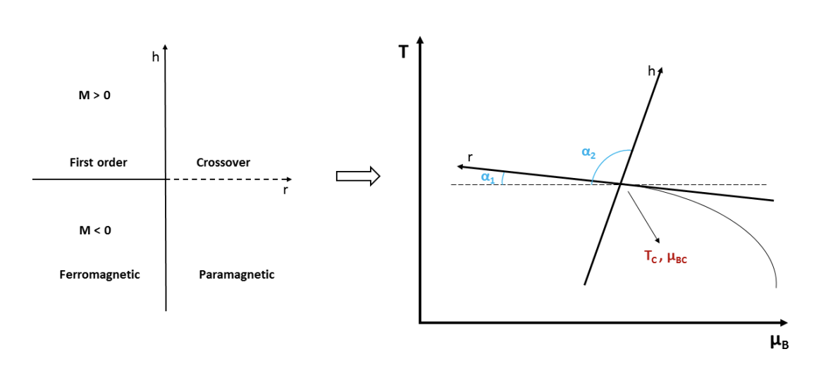
Figure 1: The mapping between QCD and Ising variables given by Eq. (2). Note that, since the sign of $h$ is a matter of convention, the mappings with $\alpha_{2}$ and $\alpha_{2}\pm\pi$ are essentially equivalent. The figure is taken from Ref. Parotto:2018pwx .

An important property of the most singular part of the Ising Gibbs free energy is scaling:

$$G(\lambda r,\lambda^{\beta\delta}h)=\lambda^{\beta(\delta+1)}G(r,h)$$ (5)

with well-known critical exponents $\beta$ and $\delta$. Another important property is the $Z_{2}$ symmetry:

$$G(r,-h)=G(r,h)\,.$$ (6)

Eqs. (5) and (6) together imply that the function $G$ can be written in terms of an even function $g$ of one variable only:

$$G(r,h)=r^{\beta(\delta+1)}g(hr^{-\beta\delta})\,.$$ (7)

The universal scaling function $g$ is multivalued. In the complex plane of its argument $x\equiv hr^{-\beta\delta}$ the primary Riemann sheet describes the equation of state at high temperatures $T>T_{c}$, i.e., $r>0$. We shall denote the value of $g$ on this sheet as $g_{+}(x)$. On the primary (high temperature) sheet the function is analytic at $x=0$. The closest singularities are on the imaginary $x$ axis and are known as Lee-Yang edge singularities Lee:1952ig ; Fisher:1978pf (see also recent discussions in Refs.Fonseca:2001dc ; An:2017brc ). A secondary Riemann sheet describes the low temperature phase, $r<0$. We shall denote the value of $g$ on this sheet as $g_{-}(x)$.

II.2 Relation between mapping parameters and derivatives of pressure

Given an equation of state $P(\mu,T)$ one should be able to determine the mapping parameters. In this Subsection, for further applications, we shall derive expressions which can be used to do that.

We shall take all derivatives of pressure below on the crossover line, i.e., at $h=0$ for $r>0$ and keep only the most singular terms. In this manuscript, a subscript with respect to $\mu$ or $T$ implies differentiation with respect to that variable when the other is kept fixed. Below, we also use indices $X$ and $Y$ to represent either $T$ or $\mu$. We find, at $h=0$:

$$P_{XY} = -Ah_{X}h_{Y}r^{\beta-\beta\delta}g_{+}^{{}^{\prime\prime}}(0)+\ldots;$$ (8)

$$P_{XXX} = 3A(\beta\delta-\beta)h_{X}^{2}r_{X}r^{\beta-\beta\delta-1}g_{+}^{{}^{\prime\prime}}(0)+\ldots;$$ (9)

$$P_{XXYY} = -Ah_{X}^{2}h_{Y}^{2}r^{\beta-3\beta\delta}g_{+}^{{}^{\prime\prime\prime\prime}}(0)+\ldots.$$ (10)

The dots represent the terms which are subleading to the terms explicitly written in the limit $r\rightarrow 0$. From the above equations, it is easy to see that

$$h_{X} = \lim_{\begin{subarray}{c}h=0\\ r\rightarrow 0^{+}\end{subarray}}\left(\frac{P_{XX}r^{\beta\delta-\beta}}{-Ag_{+}^{\prime\prime}(0)}\right)^{1/2};$$ (11)

$$r_{X} = \lim_{\begin{subarray}{c}h=0\\ r\rightarrow 0^{+}\end{subarray}}\frac{P_{XXX}r}{3(\beta-\beta\delta)P_{XX}}\,.$$ (12)

Therefore:

$$\tan\alpha_{1} =\frac{h_{\mu}}{h_{T}} =\lim_{\begin{subarray}{c}h=0\\ r\rightarrow 0^{+}\end{subarray}}\frac{P_{\mu\mu}}{P_{\mu T}}\,;$$ (13)

$$\tan\alpha_{2} =\frac{r_{\mu}}{r_{T}} =\lim_{\begin{subarray}{c}h=0\\ r\rightarrow 0^{+}\end{subarray}}\frac{P_{\mu\mu\mu}}{P_{TTT}}\frac{P_{TT}}{P_{\mu\mu}}\,.$$ (14)

Eq. (13) simply means, in particular, that the slope of the contour of critical number density ($n=P_{\mu}$) at the critical point is equal to the slope of $h=0$. Eq. (14) relates the slope of $r=0$ to the ratios of third and second derivatives of pressure evaluated along the cross-over line. These equations could be compared and contrasted with the expressions obtained by Rehr and Mermin in Ref. Rehr:1973zz using the discontinuities of the derivatives of pressure along the first-order line.

Similarly, the parameters $\rho$ and $w$ in the mapping can also be related to pressure derivatives. In order to do that we also need an expression for $r$:

$$r = \left(-\frac{g^{{}^{\prime\prime}}(0)^{2}A\,P_{\mu\mu TT}}{g^{{}^{\prime\prime\prime\prime}}(0)P_{\mu\mu}P_{TT}}\right)^{-\frac{1}{\beta(\delta+1)}}\,.$$ (15)

Using that expression in Eqs. (11) and (12) we can obtain $\rho$ and $w$ by substituting $h_{X}$ and $r_{X}$ into the following expressions:

$$\rho = \sqrt{\frac{h_{\mu}^{2}+h_{T}^{2}}{r_{\mu}^{2}+r_{T}^{2}}};$$ (16)

$$wT_{c} = \frac{\sqrt{r_{\mu}^{2}+r_{T}^{2}}}{|r_{T}h_{\mu}-r_{\mu}h_{T}|}.$$ (17)

The normalization convention in Ref. Parotto:2018pwx which we follow corresponds to $A=T_{c}^{4}/2$. Obviously, the angles $\alpha_{1}$ and $\alpha_{2}$ do not depend on this normalization whereas $\rho$ and $w$ do. To fix the normalization of $h$ and $r$ we follow the standard convention, also used in Ref. Parotto:2018pwx :

$$g_{-}^{\prime}(0^{+})=-(-1)^{\beta}\,,\qquad\lim_{x\rightarrow\infty^{+}}x^{-1/\delta}g_{\pm}^{\prime}(x)=-1\,.$$ (18)

Using equations in this subsection we can determine $\alpha_{1}$, $\alpha_{2}$, $\rho$ and $w$ if the pressure is known as a function of $\mu$ and $T$. It should be mentioned that we chose one among many ways of expressing $\alpha_{1}$, $\alpha_{2}$, $\rho$ and $w$ in terms of ratios of pressure derivatives. Our choice was guided by the desire to obtain expressions which treat $T$ and $\mu$ variables most symmetrically.

III Mean-field equation of state

III.1 Symmetry and scaling in mean-field theory

In the mean-field description of the critical point equation of state, pressure can be expressed as the minimum of the Ginzburg-Landau potential as a function of the order parameter $\phi$:

$$P(\mu,T)=-A\min_{\phi}\Omega(\phi,\mu,T)\,.$$ (19)

Let us make a simple but very useful observation: by a change of variable $\phi\to f(\phi)$ one can obtain a family of potentials $\hat{\Omega}(\phi)$ obeying $\hat{\Omega}(\phi)=\Omega(f(\phi))$ each of which gives the same pressure. We shall refer to this property as reparametrization invariance.

Close to the critical point, $\Omega$ can be expanded around the critical value of $\phi$ (chosen to be $\phi=0$):

$$\Omega(\phi,\mu,T)=\Omega_{0}-h\phi+\frac{r}{2}\phi^{2}+\frac{u}{4}\phi^{4}+\ldots\,,$$ (20)

where we eliminated cubic term $\phi^{3}$ by a shift of variable $\phi$ (such an operator or term is called redundant in renormalization group terminology). Parameters $\Omega_{0}$, $h$, $r$ and $u$ are analytic functions of $\mu$ and $T$. The critical point is located at $h=0$ and $r=0$ (with $u>0$). If we truncate the expansion at order $\phi^{4}$ as in Eq. (20) the $\phi$-dependent part, $\Omega-\Omega_{0}$, possesses two important properties. The first is the $Z_{2}$ symmetry:

$$\phi\to-\phi,\quad h\to-h,\quad r\to r\,.$$ (21)

The second is scaling:

$$\phi\sim r^{1/2},\quad h\sim r^{3/2},\quad\Omega-\Omega_{0}\sim r^{2}\,.$$ (22)

This corresponds to the scaling of the Gibbs free energy $G$ in Eq. (5) with mean-field exponents $\beta=1/2$ and $\beta\delta=3/2$.

One could be tempted to expand the coefficients $h$ and $r$ in Eq. (20) to linear order in $\Delta T$ and $\Delta\mu$ and identify the mixing parameters $\alpha_{1}$, $\alpha_{2}$, etc., by using Eq. (2). This, however, is not entirely correct as it would ignore the fact that the mixing of $h$ and $r$ described by Eq. (2) necessarily violates scaling, since $h\sim r^{3/2}$ and $r$ have different scaling exponents. Therefore, we need also to look at the omitted terms which violate scaling in Eq. (20), or more precisely, provide corrections to scaling of relative order $h/r\sim r^{1/2}$ (i.e., $r^{\beta\delta-1}$). Furthermore, mixing of $h$ and $r$ also violates $Z_{2}$ symmetry in Eq. (21), i.e., we need also to look at omitted $Z_{2}$ breaking terms in Eq. (20).

Since $\phi\sim r^{1/2}$, omitted higher order terms in Eq. (20) represent corrections to scaling. The leading correction is due to the $\phi^{5}$ term. Because in mean-field theory this term is smaller by exactly a factor of $r^{1/2}$ compared to the terms in Eq. (20), and also because it violates the $Z_{2}$ symmetry in Eq. (21) (being odd), this term will affect the mixing of $h$ and $r$.

III.2 The effect of the $\phi^{5}$ term

Let us denote the coupling of the $\phi^{5}$ term by $vu$, i.e.,

$$\Omega=\Omega_{0}-{\bar{h}}\phi+\frac{1}{2}{\bar{r}}\phi^{2}+\frac{u}{4}\phi^{4}+vu\phi^{5}+O(\phi^{6}),$$ (23)

where we also changed the notation for the coefficients of the $\phi$ and $\phi^{2}$ terms in anticipation of them being different from $h$ and $r$ in Eq. (2).

To understand the effect of the $\phi^{5}$ term on the mixing of $h$ and $r$ we can use reparametrization invariance of pressure to change the variable $\phi$ in such a way as to eliminate the $\phi^{5}$ term from $\Omega$. This can be achieved by the following transformation:

$$\phi\to\phi+v\left(\frac{{\bar{r}}}{u}-\phi^{2}\right)\,,$$ (24)

which eliminates $\phi^{5}$ and as well as $\phi^{3}$ term at order up to $r^{5/2}$:

$$\Omega=\left(\Omega_{0}-\frac{v{\bar{h}}{\bar{r}}}{u}\right)-\left({\bar{h}}-\frac{v{\bar{r}}^{2}}{u}\right)\phi+\left(\frac{{\bar{r}}}{2}+v{\bar{h}}\right)\phi^{2}+\frac{u}{4}\phi^{4}+\mathcal{O}(\phi^{6},r^{3})\,,$$ (25)

where we kept only terms up to order $r^{5/2}$, since we are interested in the leading correction to scaling. From Eq. (25) we can now read off the parameters $h$ and $r$:

$$h = u^{-1/4}\left({\bar{h}}-\frac{v{\bar{r}}^{2}}{u}\right)=u^{-1/4}{\bar{h}}+\mathcal{O}({\bar{r}}^{2}),$$ (26)

$$r = u^{-1/2}\left({\bar{r}}+2v{\bar{h}}\right),$$ (27)

which match Eq. (25) onto a mean-field potential without leading asymmetric ($Z_{2}$-breaking, non-Ising) corrections to scaling. The additional rescaling $\phi\to u^{-1/4}\phi$ was applied to bring the potential to the canonical form:

$$\Omega=-h\phi+\frac{r}{2}\phi^{2}+\frac{1}{4}\phi^{4}.$$ (28)

The scaling function $g(x)$ corresponding to this potential via $G=\min_{\phi}\Omega=r^{2}g(hr^{-3/2})$ (see Eq. (7)) satisfies

$$x+g^{\prime}(x)+g^{\prime 3}(x)=0,$$ (29)

which agrees with the normalization in Eq. (18). Therefore, parameters $h$ and $r$ in Eqs. (26) and (27) are the parameters which appear in the mapping equations (2).

Note that the main effect of the asymmetric corrections to scaling is to modify ${\bar{r}}$ in Eq. (27) by a term linear in ${\bar{h}}$, which has direct effect on the angle $\alpha_{2}$ determining the slope of the $r=0$ axis. The slope of the $h=0$ axis is not affected as the shift of ${\bar{h}}$ in Eq. (26) is quadratic in ${\bar{r}}$.

III.3 Direct relation to derivatives of the potential

It is also useful to relate mapping parameters $h_{X}$ and $r_{X}$, where $X=T$ or $\mu$, directly to the Ginzburg-Landau potential $\Omega$. The relation can be obtained straightforwardly from Eqs. (8-10) using

$$P_{XX} = -\Omega_{XX}+\Omega_{X\phi}^{2}\Omega_{\phi\phi}^{-1}\,,$$ (30)

$$P_{XXX} = -\Omega_{XXX}-3\Omega_{\phi\phi}^{-2}\Omega_{X\phi}(\Omega_{X\phi}\Omega_{X\phi\phi}-\Omega_{\phi\phi}\Omega_{XX\phi})+\Omega_{\phi X}^{3}\Omega_{\phi\phi}^{-3}\Omega_{\phi\phi\phi}\,.$$ (31)

To simplify the expressions we shall first consider potential $\hat{\Omega}$ obtained from $\Omega$ by bringing it into the “Ising” form in Eq. (20) with no $\phi^{3}$ or $\phi^{5}$ terms (up to order $r^{5/2}$). We showed that this can be always achieved by a reparametrization as in Eq. (24), Eq. (25). In this case, $\hat{\Omega}_{\phi\phi\phi}=0$ on the $h=0$ line along which we take the limits in Eqs. (11), (12) and expressions simplify:

$$\tan\alpha_{1} = \frac{\hat{\Omega}_{\phi\mu}}{\hat{\Omega}_{\phi T}}\,;$$ (32)

$$\tan\alpha_{2} = \frac{\hat{\Omega}_{\phi\phi\mu}}{\hat{\Omega}_{\phi\phi T}}\,;$$ (33)

$$\rho = \left(\frac{\hat{\Omega}_{\phi\phi\phi\phi}}{6}\right)^{1/4}\sqrt{\frac{\hat{\Omega}_{\phi\mu}^{2}+\hat{\Omega}_{\phi T}^{2}}{\hat{\Omega}_{\phi\phi\mu}^{2}+\hat{\Omega}_{\phi\phi T}^{2}}}\,;$$ (34)

$$wT_{c} = \left(\frac{\hat{\Omega}_{\phi\phi\phi\phi}}{6}\right)^{1/4}\frac{\sqrt{\hat{\Omega}_{\phi\phi\mu}^{2}+\hat{\Omega}_{\phi\phi T}^{2}}}{|\hat{\Omega}_{\phi\mu}\hat{\Omega}_{\phi\phi T}-\hat{\Omega}_{\phi T}\hat{\Omega}_{\phi\phi\mu}|}\,.$$ (35)

Note that in the mean-field theory these expressions are analytic at the critical point and can be simply evaluated at the critical point without taking a limit. This is in contrast to Eqs. (11) and (12) where the derivatives of pressure are singular and a careful limit has to be taken to cancel singularities.

One can then generalize these expressions to arbitrary potential ($\Omega_{\phi\phi\phi}\neq 0$ at $h=0$) by observing that combinations

$$\Omega_{\phi X},\quad\Omega_{\phi\phi X}-\frac{\Omega_{\phi\phi\phi\phi\phi}\Omega_{\phi X}}{10\Omega_{\phi\phi\phi\phi}},\quad\mbox{and}\quad\Omega_{\phi\phi\phi\phi},$$ (36)

are reparametrization “covariant” to leading order in $r$ in the sense that under $\phi\to f(\phi)$ they transform multiplicatively by factors $f^{\prime}$, $(f^{\prime})^{2}$ and $(f^{\prime})^{4}$, respectively. Thus, we can drop ‘hats’ and replace

$$\hat{\Omega}_{\phi\phi X}\to\Omega_{\phi\phi X}-\frac{\Omega_{\phi\phi\phi\phi\phi}\Omega_{\phi X}}{10\Omega_{\phi\phi\phi\phi}}$$ (37)

in Eqs. (32-35) to obtain general formulas applicable to any potential. Note that the last term in Eq. (37) corresponds to the last term in Eq. (27) describing the mixing of $r$ and $h$ due to the $\phi^{5}$ term.

IV Critical point near a tricritical point

A tricritical point arises in many systems where the order of the finite-temperature transition from broken to restored symmetry phase depends on an additional thermodynamic parameter, such as pressure or chemical potential. The point where the order of the transition changes from second to first is a tricritical point. There are reasons to believe QCD to be one of the examples of such a theory Stephanov:1998dy ; Stephanov:2004wx . A nonzero value of a parameter which breaks spontaneously broken symmetry explicitly (quark mass in QCD) removes the second order phase transition and replaces it with analytic crossover, while the first order transition then ends at a critical point.

We shall apply mean-field theory near the tricritical point. The potential needed to describe the change from a first to second order transition needs to include a $\Phi^{6}$ term which becomes marginal in $d=3$. Therefore, mean field theory should be applicable in $d=3$ if one is willing, as we are, to neglect small logarithmic corrections to scaling.

As in Section III we want to express the pressure as a minimum of the Ginzburg-Landau potential $\Omega$. We can do that using the Legendre transform of pressure $P$ with respect to $m_{q}$:

$$V(\Phi,\mu,T)=-P(\mu,T,m_{q}(\Phi))+m_{q}(\Phi)\Phi\,,$$ (38)

where $m_{q}(\Phi)$ is the solution of

$${\partial P}/{\partial m_{q}}=\Phi,$$ (39)

which means $\Phi$ is the chiral condensate (times $N_{f}$ – the number of light quarks).

It is easy to see that the potential $\Omega$ defined as

$$A\Omega(\Phi,\mu,T,m_{q})=V(\Phi,\mu,T)-m_{q}\Phi$$ (40)

is related to pressure by

$$P(\mu,T,m_{q})=-A\min_{\Phi}\Omega(\Phi,\mu,T,m_{q})$$ (41)

where we chose the normalization constant $A$ to match Eq. (19).

The potential $V$ has to be symmetric under $\Phi\rightarrow-\Phi$ (this is a discrete subgroup of the continuous chiral symmetry) and to describe a tricritical point we need terms up to $\Phi^{6}$. Expanding $V$ we find:

$$V(\Phi,\mu,T)=V_{0}+\frac{a}{2}\Phi^{2}+\frac{b}{4}\Phi^{4}+\frac{c}{6}\Phi^{6}+\ldots\,,$$ (42)

where $a$, $b$ and $c$ are functions of $T$ and $\mu$. The tricritical point occurs when $a=b=0$ with $c>0$. If we truncate $V$ at order $\Phi^{6}$ as in Eq. (42) the $\Phi$-dependent part of $V$ and $\Omega$, has the following scaling property:

$$\Phi\sim a^{1/4},\quad b\sim a^{1/2},\quad m_{q}\sim a^{5/4}\quad V-V_{0}\sim a^{3/2}\,.$$ (43)

The minimum value of $\Omega$ in Eq. (41) is achieved at $\Phi$ satisfying, to lowest order in $a\to 0$,

$$m_{q}=\frac{\partial{V}}{\partial\Phi}=a\Phi+b\Phi^{3}+c\Phi^{5}\,.$$ (44)

At nonzero $m_{q}$ the critical point occurs when both second and third derivatives of $\Omega$ vanish at the minimum given by Eq. (44). I.e.,

$$\frac{\partial^{2}{V}}{\partial\Phi^{2}}=\frac{\partial m_{q}}{\partial\Phi}=a+3b\Phi^{2}+5c\Phi^{4}=0.$$ (45)

and

$$\frac{\partial^{3}{V}}{\partial\Phi^{3}}=6b\Phi+20c\Phi^{3}=0.$$ (46)

Eqs. (44), (45) and (46), can be solved simultaneously to find the critical values of $\Phi$, $a$ and $b$ for a given $m_{q}$:

$$\Phi_{c}=\left(\frac{3m_{q}}{8c}\right)^{1/5},\quad a_{c}=5c\Phi_{c}^{4},\quad b_{c}=-\frac{10c}{3}\Phi_{c}^{2}.$$ (47)

As a function of $m_{q}$, the trajectory $(m_{q},a_{c}(m_{q}),b_{c}(m_{q}))$ corresponds to the line of critical points on the edges of “wings” – coexistence surfaces in the $m_{q}$, $T$, $\mu$ phase diagram (see, e.g., Fig. 3 for illustration). Note that critical values of parameters in Eq. (47) scale as $\Phi_{c}\sim m_{q}^{1/5},a_{c}\sim m_{q}^{4/5}$ and $b_{c}\sim m_{q}^{2/5}$ consistent with the scaling in Eq. (43). We can now expand $\Omega$ around that solution:

$$A\,\Omega(\Phi;\mu,T,m_{q})=A\,\Omega(\Phi_{c};T_{c},\mu_{c},m_{q})+(\Delta a\Phi_{c}+\Delta b\Phi_{c}^{3})\phi+\frac{1}{2}(\Delta a+3\Delta b\Phi_{c}^{2})\phi^{2}+\frac{1}{4}\left(\frac{20c\Phi_{c}^{2}}{3}+\Delta b\right)\phi^{4}\\ +\Delta b\Phi_{c}\phi^{3}+c\Phi_{c}\phi^{5}+\frac{c}{6}\phi^{6}\,,$$ (48)

where $\Delta a=a-a_{c}$, $\Delta b=b-b_{c}$ and $\phi=\Phi-\Phi_{c}$. We can now compare this expansion to the $\phi^{4}$ theory in the previous section. The redundant term $\phi^{3}$ can be eliminated, as usual, by a shift of $\phi$. Comparing with Eq. (23) we find:

$$A\,{\bar{h}} = -(\Delta a+\Delta b\Phi_{c}^{2})\Phi_{c}\,,$$ (49)

$$A\,{\bar{r}} = \Delta a+3\Delta b\Phi_{c}^{2}\,,$$ (50)

$$Au = \frac{20\Phi_{c}^{2}}{3}\,,\quad v=\frac{3}{20\Phi_{c}}\,.$$ (51)

The $\phi^{5}$ term causes mixing of ${\bar{h}}$ and ${\bar{r}}$ as in Eq. (27). Using Eqs. (26) and (27) to linear order in $\Delta a$ and $\Delta b$ (i.e., linear order in $\Delta T$ and $\Delta\mu$) we find

$$A\,h=-u^{-1/4}\,\left(\Delta a+\Delta b\Phi_{c}^{2}\right)\Phi_{c},$$ (52)

$$A\,r=u^{-1/2}\left(\frac{7}{10}\Delta a+\frac{27}{10}\Delta b\Phi_{c}^{2}\right).$$ (53)

Since $a$ and $b$ are analytic functions of $T$ and $\mu$ near the critical point we can expand to linear order:

$$\Delta a=a_{T}\Delta T+a_{\mu}\Delta\mu\,;$$

$$\Delta b=b_{T}\Delta T+b_{\mu}\Delta\mu\,.$$ (54)

Using Eqs. (32), (33), we determine the slopes at the critical point:

$$\tan\alpha_{1} = -\left(\frac{dT}{d\mu}\right)_{h=0}=\frac{h_{\mu}}{h_{T}}=\frac{a_{\mu}+b_{\mu}\Phi_{c}^{2}}{a_{T}+b_{T}\Phi_{c}^{2}}\,;$$ (55)

$$\tan\alpha_{2} = -\left(\frac{dT}{d\mu}\right)_{r=0}=\frac{r_{\mu}}{r_{T}}=\frac{a_{\mu}+27b_{\mu}\Phi_{c}^{2}/7}{a_{T}+27b_{T}\Phi_{c}^{2}/7}\,.$$ (56)

In general, the two slopes are different and non-universal (i.e., depend on the non-universal coefficients $a_{\mu}$, $a_{T}$, etc. However, the limit $m_{q}\to 0$ is special. In this limit the two slopes approach each other with the difference vanishing as $\Phi_{c}^{2}\sim m_{q}^{2/5}$ (see Eq. (47)):

$$\tan\alpha_{1}-\tan\alpha_{2}=\left(\frac{dT}{d\mu}\right)_{r=0}-\left(\frac{dT}{d\mu}\right)_{h=0} = \frac{20}{7a_{T}^{2}}\frac{\partial(a,b)}{\partial(\mu,T)}\Phi_{c}^{2}+\mathcal{O}(\Phi_{c}^{4})$$ (57)

$$= \frac{20}{7a_{T}^{2}}\frac{\partial(a,b)}{\partial(\mu,T)}\left(\frac{3}{8c}\right)^{2/5}m_{q}^{2/5}+\mathcal{O}(m_{q}^{4/5})\,,$$

where ${\partial(a,b)}/{\partial(\mu,T)}=a_{\mu}b_{T}-a_{T}b_{\mu}$ is the Jacobian of the mapping in Eq. (54).

The relative orientation of the slopes, i.e., the sign of the slope difference, is determined by the sign of the Jacobian of the $(a,b)\to(\mu,T)$ mapping. It is positive in the case of the mapping without reflection and negative otherwise. In that sense, it is topological. We show how to determine the sign on Fig. 2 by comparing the phase diagram in the vicinity of the tricritical point in $(a,b)$ coordinates with the standard scenario of the QCD phase diagram in $(\mu,T)$ coordinates. We see that the two graphs are topologically the same: the first order transition is to the right of the tricritical point and the broken (order) phase is below the tricritical point. This means that the Jacobian of the $(a,b)$ to $(\mu,T)$ is positive (no reflection is involved). This means that, since $h=0$ slope is negative, the $r=0$ slope must be less steep, or if $\alpha_{1}$ itself is small, $\alpha_{2}$ could be slightly negative. We shall see in the next Section that in the random matrix model both slopes are negative and small (i.e., $\alpha_{1}>\alpha_{2}>0$ in the model).

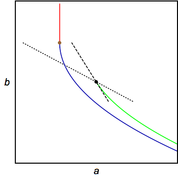
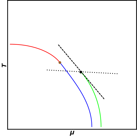
Figure 2: Left: The phase diagram of the $\Phi^{6}$ theory described by Eq. (48) in the $a-b$ plane. Right: QCD phase diagram in the $\mu-T$ plane. The blue and red lines correspond to the first-order and second-order phase transitions at $m_{q}=0$ respectively. They join at a tricritical point. The green line represents the first-order phase transition at $m_{q}\neq 0$ ending in a critical point. The symmetry broken (ordered) phase is in the lower left corner in both cases. The slopes of the $h=0$ and $r=0$ lines at the critical point are indicated by the dashed and dotted lines respectively.

The Jacobian in Eq. (89) can be rewritten in a more geometrically intuitive form in terms of the difference of slopes of $a=0$ and $b=0$ on the $(\mu,T)$ phase diagram of QCD at $m_{q}=0$:

$$\frac{1}{a_{T}^{2}}\frac{\partial(a,b)}{\partial(\mu,T)}=\left(\frac{\partial b}{\partial a}\right)_{\mu}\left(\left(\frac{\partial T}{\partial\mu}\right)_{b=0}-\left(\frac{\partial T}{\partial\mu}\right)_{a=0}\ \right)\,.$$ (58)

The $a=0$ slope is, of course, the slope of the chiral phase transition line at the tricritical point.

One can also determine the dependence of $\rho$ and $w$ on $m_{q}$ using Eqs. (34) and (35). Using Eq. (48) we find, in the limit of $m_{q}\rightarrow 0$:

$$\sqrt{\Omega^{{}^{2}}_{\phi\mu}+\Omega^{{}^{2}}_{\phi T}}\sim m_{q}^{1/5},\quad\sqrt{\Omega^{{}^{2}}_{\phi\phi\mu}+\Omega^{{}^{2}}_{\phi\phi T}}\sim m_{q}^{0},$$

$$\Omega_{\phi\mu}\Omega_{\phi\phi T}-\Omega_{\phi\mu}\Omega_{\phi\phi T}\sim m_{q}^{3/5},\quad\Omega_{\phi\phi\phi\phi}\sim m_{q}^{2/5}\,,$$ (59)

and thus

$$\rho\sim m_{q}^{3/10},\qquad w\sim m_{q}^{-1/2}.$$ (60)

V Random Matrix Model

To illustrate the general results derived in the previous section we consider the random matrix model (RMM) introduced by Halasz et al in Ref. Halasz:1998qr in order to describe the chiral symmetry restoring phase transition in QCD. This is a mean-field model which has features similar to the effective Landau-Ginsburg potential near a tricritical point discussed in the previous section. The QCD pressure in this model is given by

$$P(\mu,T,m_{q})=-\mathpzc{N}\min_{\phi}\Omega^{RMM}(\Phi;\mu,T,m_{q})\,,$$ (61)

where

$$\Omega^{RMM}(\Phi;\mu,T,m_{q})=\Phi^{2}-\frac{1}{2}\ln\left\{\left[\left(\Phi+m_{q}\right)^{2}-\left(\mu+iT\right)^{2}\right].\left[\left(\Phi+m_{q}\right)^{2}-\left(\mu-iT\right)^{2}\right]\right\}$$ (62)

and $\mathpzc{N}=n_{\text{inst}}N_{f}$ where $n_{\text{inst}}\approx 0.5fm^{-4}$ is the typical instanton number 4-density and $N_{f}=2$ is the number of flavors of light quarks. The units for $T,\mu$ and $m_{q}$ here are such that $T=1$, $\mu=1$ and $m_{q}=1$ in these units correspond to approximately $160\,\text{MeV}$, $2300\,\text{MeV}$ and $100\,\text{MeV}$ respectively (as in Ref. Halasz:1998qr ).

To use the results of the previous section we identify

$$A\Omega(\Phi;\mu,T,m_{q})=\mathpzc{N}\Omega^{RMM}(2\Phi;\mu,T,m_{q})\,,$$ (63)

which takes into account that $\partial\Omega^{RMM}/\partial m_{q}=2\Phi$.

The equation of state that follows from this potential, $\partial\Omega/\partial\Phi=0$, is a fifth order polynomial equation. The phase diagram resulting from this potential is shown in Fig. 3.

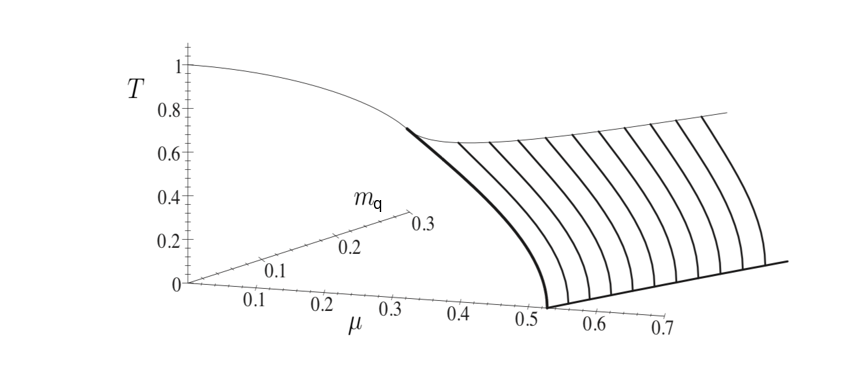
Figure 3: The phase diagram for the random matrix model in Ref. Halasz:1998qr . On the $m_{q}=0$ plane, the thick and the thin lines represent the first-order and the second-order phase transitions respectively. Upon turning on $m_{q}$, the tricritical point where these two lines meet turns into a line of Ising-like critical points $(\mu_{c}(m_{q}),T_{c}(m_{q}))$. For the discussion that follows, we fix $m_{q}$ to a particular value and obtain the map from $(\mu-\mu_{c}(m_{q}),T-T_{c}(m_{q}))$ to $(h,r)$ variables.

The tricritical point for this model is at $(\mu_{3},T_{3})=\left(\sqrt{-1+\sqrt{2}},\sqrt{1+\sqrt{2}}\right)/2$. Expanding the potential given by Eq. (62) we find

$$\mathpzc{N^{-1}}A\,\Omega(\Phi;\mu,T)=\mathpzc{N^{-1}}A\,\Omega(0;\mu,T)+\frac{a}{2}\Phi^{2}+\frac{b}{4}\Phi^{4}+\frac{c}{6}\Phi^{6}-d\Phi+\ldots,$$ (64)

where

$$a=\frac{1}{2}\left(\frac{\mu^{2}-T^{2}}{\left(\mu^{2}+T^{2}\right)^{2}}+1\right);\quad b=\frac{\mu^{4}+T^{4}-6\mu^{2}T^{2}}{8\left(\mu^{2}+T^{2}\right)^{4}};$$ (65)

$$c=\frac{\left(\mu^{2}-T^{2}\right)\left(\mu^{4}+T^{4}-14\mu^{2}T^{2}\right)}{32\left(\mu^{2}+T^{2}\right)^{6}};\quad d=m_{q}\frac{T^{2}-\mu^{2}}{\left(T^{2}+\mu^{2}\right)^{2}},$$ (66)

and dots denote terms such as $\Phi^{8}$, $m_{q}\Phi^{3}$, etc., which are of order $a^{2}$ and smaller, negligible compared to the terms kept (which are of order $a^{3/2}$), according to the scaling in Eq. (43).

For a given $m_{q}$, the critical values $\Phi_{c},\mu_{c}$ and $T_{c}$ are obtained by simultaneously requiring the first, second and third derivatives of $\Omega$ with respect to $\Phi$ to vanish. As $m_{q}\rightarrow 0$,

$$\mu_{c}(m_{q})=\mu_{3}+O(m_{q}^{2/5})\,,\quad T_{c}(m_{q})=T_{3}+O(m_{q}^{2/5})\,,\quad\Phi_{c}(m_{q})=\left(6m_{q}\right)^{1/5}+O(m_{q}^{3/5})$$ (67)

Using Eq. (57), we can now obtain the slope difference:

$$\tan\alpha_{1}-\tan\alpha_{2} = \frac{20}{7}(2+\sqrt{2})(6m_{q})^{2/5}+\mathcal{O}(m_{q}^{4/5})\,.$$ (68)

As $m_{q}\rightarrow 0$, the lines $h=0$ and $r=0$ become nearly parallel to each other with the difference in their slopes being proportional to $m_{q}^{2/5}$ as predicted in the previous section. Comparing Eq. (68) to Eq. (57), one can see that $\partial(a,b)/\partial(\mu,T)$ is positive, as expected.

Using more general (finite $m_{q}$) Eqs. (32-35,37) we computed the vales for the parameters $\alpha_{1}$, $\alpha_{2}$, $\rho$ and $w$ at $m_{q}=0.05$ (which corresponds to quark masses of 5 MeV in the units of Ref. Halasz:1998qr ) in RMM:

$$\alpha_{1}\sim 13^{\circ},\quad\alpha_{2}\sim 1^{\circ},\quad\rho\sim 0.5,\quad w\sim 1.4\,.$$ (69)

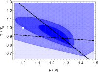
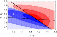
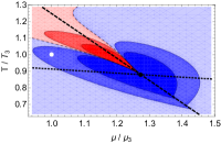
Figure 4: Contour plots of susceptibilities $\chi_{2}=P_{\mu\mu}$, $\chi_{3}=P_{\mu\mu\mu}$ and $\chi_{4}=P_{\mu\mu\mu\mu}$ near the critical point corresponding to $m_{q}=0.05$ in the RMM. The black and white dots represent the critical point and the tricritical point (at $m_{q}=0$) respectively. The dotted and the dashed lines are the $r=0$ and $h=0$ lines respectively. The slope of $r=0$ is negative for this value of $m_{q}$. The negative valued regions are red and positive valued regions are blue. Note that the value of $\chi_{3}$ along the $h=0$ line on the cross-over side is negative.

The contour plots of singular pressure derivatives $\chi_{2}=P_{\mu\mu}$, $\chi_{3}=P_{\mu\mu\mu}$ and $\chi_{4}=P_{\mu\mu\mu\mu}$ (baryon number cumulants, or susceptibilities, of second, third and fourth order) around the critical point at small quark mass are shown in Fig. 4. The following observations can be made:

• The slopes of $h=0$ and $r=0$ are both negative and $h=0$ axis (coexistence line) is steeper than than $r=0$ axis.

• $\rho<w$, which is in qualitative agreement with the small $m_{q}$ scaling in Eqs. (60).

• The signs of the cumulants $\chi_{2}$ and $\chi_{4}$ on the crossover side of $h=0$ line are in agreement with Eqs. (8) and (10) with $g_{+}^{\prime\prime}(0)=-1<0$ and $g_{+}^{\prime\prime\prime\prime}(0)=6>0$ according to Eq. (29).

• Most interestingly, the sign of $\chi_{3}$ on the crossover side of $h=0$ line, according to Eq. (9), is determined by the sign of $-r_{\mu}$. This is clearly seen in Fig. 4b where $\chi_{3}<0$ in accordance to $r_{\mu}>0$ ($\alpha_{2}>0$). If the same holds true in QCD, this may have phenomenological consequences as the sign of cubic cumulant (skewness) is measured in heavy-ion collisions (see also discussion in Section VII).

RMM is a model of QCD, capturing some of its physics, such as chiral symmetry breaking, and missing other features, such as confinement. Its results should be treated with caution to avoid mistaking artifacts for physics. The behavior of the equation of state near the tricritical point is, however, subject to universality constraints, which we verified are satisfied by the model. The numerical values for the mapping parameters we obtained in Eq. (69) should be treated as estimates, or informed guesses. These parameters are not universal. However, their dependence on $m_{q}$ is universal, and is manifested in RMM (e.g., the slope difference is small and $\rho<w$ in accordance with Eqs. (60)). Since no other information about these parameters is available as of this writing, we believe our estimates in Eq. (69) could be helpful for narrowing down the parameter domain of the approximate equations of state constructed along the lines of Ref. Parotto:2018pwx .

VI Beyond the mean-field theory

In Sections III-V, we discussed the mean-field theory near a critical point. Within such a theory, we derived scaling relations for $\tan\alpha_{1}-\tan\alpha_{2}$, $\rho$ and $w$ in the $m_{q}\rightarrow 0$ limit in Eqs. (57) and (60). The mean-field theory should break down sufficiently close to the critical point in $d=3$ dimensions since the upper critical dimension near a critical point is $d=4$. The breakdown occurs because contribution of fluctuations increases with increasing correlation length $\xi$ (the fluctuations become coherent at larger scales). The extent of the region where the mean-field theory breaks down can be estimated using the Ginsburg criterion by comparing the strength of the one-loop correction (infrared-divergent for $d<4$) to the coupling to its tree-level value as shown in Fig. 5.

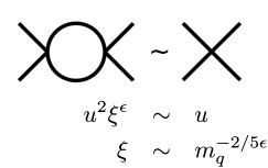
Figure 5: The one-loop contribution of fluctuations compared to the tree-level coupling. The fluctuation contribution diverges as $\xi^{\epsilon}$, where $\epsilon=4-d$. The mean-field approximation breaks down at sufficiently large $\xi$ when the contribution of fluctuations is no longer negligible. The scaling of $u\sim\Phi_{c}^{2}\sim m_{q}^{2/5}$ follows from Eq. (48).

Since the mean-field limit is essentially weak-coupling limit, a quicker argument is to compare the coupling $u$ expressed in dimensionless units, i.e., $u\xi^{\epsilon}$, where $\epsilon=4-d$ is the mass dimension of $u$, to unity. Since in the mean-field region $h\sim\xi^{-3}$ and $r\sim\xi^{-2}$, the boundary of the Ginsburg region where the mean-field theory breaks down is parametrically given by $h_{G}\sim m_{q}^{6/5}$, $r_{G}\sim m_{q}^{4/5}$ in $d=3$. Note that the Ginzburg region is parametrically small for small $m_{q}$. It is also parametrically smaller than the distance between the critical and the tricritical points $b_{c}\sim m_{q}^{2/5}$, Eq. (47). The characteristic size and shape of the Ginzburg region is illustrated in Fig. 6.

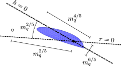
Figure 6: Schematic representation of the scaling of various parameters characterizing the location, the size and the shape of the Ginzburg region (shown in blue) around the QCD critical point in the $T$ vs $\mu$ plane for small quark mass $m_{q}$. The empty circle denotes the location of the tricritical point at $m_{q}=0$. The dotted and dashed lines are the $r=0$ and $h=0$ axes, respectively, with an angle between them vanishing as $m_{q}^{2/5}$ in the chiral limit.

In this section we study the effects of the fluctuations to see if and how our mean-field results are modified in the Ginzburg region. We are going to use $\epsilon$ expansion to order $\epsilon^{2}$ to address this question. We shall focus on our main result – the convergence of the $r=0$ and $h=0$ slopes in the chiral limit $m_{q}\to 0$ described by Eq. (57).

The result we derived using mean-field theory could be potentially modified if the contributions of the fluctuations modify the expression for $\bar{r}$ in Eq. (50). An obvious contribution to the $\phi^{2}$ in the effective potential $\Omega$ comes from a tadpole diagram. This correction, however, does not break the $Z_{2}$ symmetry which is necessary to induce the additional mixing of $r$ and $h$ needed to change the direction of the $r=0$ axis. 

Therefore, to induce $r-h$ mixing via fluctuations we would need a $Z_{2}$ breaking term. Furthermore, $r-h$ mixing violates scaling, since $h\sim r^{\beta\delta}$ and thus we need terms which violate scaling by $r^{\beta\delta-1}$. In mean-field theory this corresponds to scaling violations of order $r^{1/2}$, which are produced by terms in the potential $\Omega$ which scale as $r^{5/2}$, i.e., operators of dimension 5. We have already seen how operator $\phi^{5}$ induces $r-h$ mixing in Section III. Here we need to generalize this discussion to include effects of fluctuations.

As usual, we start at the upper critical dimension $d=4$ and then expand in $\epsilon=4-d$. When $\phi$ is a fluctuating field, in $d=4$, the scaling part of the potential $\Omega$ also includes additional dimension 4 operator, $(\nabla\phi)^{2}$, i.e.,

$$\Omega=\frac{1}{2}(\nabla\phi)^{2}+\frac{{\bar{r}}}{2}\phi^{2}+\frac{u}{4}\phi^{4}-{\bar{h}}\phi+\ldots\,,$$ (70)

where ellipsis denotes higher-dimension operators. While $\phi^{5}$ is the only dimension five $Z_{2}$ breaking term in the mean-field theory, when fluctuations of $\phi$ are considered there are two such terms: $\phi^{5}$ and $\phi^{2}\nabla^{2}\phi$. However, we shall see that only one special linear combination of these terms has the scaling property needed to induce $r-h$ mixing when $d<4$.

To identify this linear combination let us observe that using the transformation of variables $\phi\rightarrow\phi+\Delta\phi$, where $\Delta\phi=-v(\phi^{2}-{\bar{r}}/u)$ similar to Eq. (24), we can cancel a certain linear combination of $\phi^{5}$ and $\phi^{2}\nabla^{2}\phi$, while introducing additional $\phi^{2}$ term:

$$\Delta\Omega=\Delta\phi\frac{\partial\Omega}{\partial\phi}=-v\left(u\phi^{5}-\phi^{2}\nabla^{2}\phi\right)+v{\bar{h}}\phi^{2}+\dots\,,$$ (71)

where ellipsis denotes terms which do not affect the mapping (being nonlinear in ${\bar{r}}$ or simply total derivatives). Therefore, the effect of the perturbation $vV_{3}$, where

$$V_{3}=u\phi^{5}-\phi^{2}\nabla^{2}\phi\,,$$ (72)

is equivalent to the shift ${\bar{r}}\to{\bar{r}}+2v{\bar{h}}$. The correction to scaling induced in $G$ due to a perturbation $v_{3}V_{3}$ can be absorbed by “revised scaling”

$$G({\bar{r}},{\bar{h}})={\bar{r}}^{\beta(\delta+1)}\left(g({\bar{h}}{\bar{r}}^{-\beta\delta})+v_{3}{\bar{r}}^{\Delta_{3}}g_{3}({\bar{h}}{\bar{r}}^{-\beta\delta})\right)+\ldots=r^{\beta(\delta+1)}g(hr^{-\beta\delta})+\ldots\,,$$ (73)

where

$$r={\bar{r}}+2v_{3}{\bar{h}}\quad\mbox{and}\quad h={\bar{h}}.$$ (74)

This property also guarantees Nicoll:1981zz ; Amit:1984ms that operator $V_{3}$ is an eigenvector of the RG matrix of anomalous dimensions which mixes $u\phi^{5}$ and $\phi^{2}\nabla^{2}\phi$. The corresponding correction-to-scaling exponent is given by Nicoll:1981zz ; Brezin:1972fc

$$\Delta_{3}=\beta\delta-1=1/2+\mathcal{O}(\epsilon^{2})\,,$$ (75)

which is simply the difference between $h$ and $r$ scaling exponents, as expected, since $V_{3}$ induces $r-h$ mixing.

The other eigenvalue of the anomalous dimension matrix is

$$\Delta_{5}=1/2+\epsilon+\mathcal{O}(\epsilon^{2})\,,$$ (76)

and the corresponding eigenvector is

$$V_{5}\equiv u\phi^{5}-(10S_{5}/3)\phi^{2}\nabla^{2}\phi.$$ (77)

The mixing parameter $S_{5}$ has been calculated in Ref. Nicoll:1981zz :

$$S_{5}=-\epsilon/108+\mathcal{O}(u),$$ (78)

where, consistent with our interest in the $m_{q}\to 0$ limit, we assumed that $u\ll\epsilon$, since $u\sim m_{q}^{2/5}$. The eigenvalue degeneracy is lifted at one-loop order, however, the mixing only appears at two-loop order due to the sunset diagram shown in Fig. 7. Despite the diagram being of order $\epsilon^{2}$, the mixing, i.e., $S_{5}$, is of order $\epsilon^{2}/(\Delta_{5}-\Delta_{3})=\mathcal{O}(\epsilon)$.

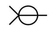
Figure 7: The two-loop diagram responsible for the mixing of $\phi^{5}$ and $\phi^{2}\nabla^{2}\phi$ operators.

In the case of physical interest, $d=3$, the values of the exponents $\Delta_{3}$ and $\Delta_{5}$ are significantly different. The exponents $\beta$ and $\delta$ are fairly well known and have been determined using different methods, including experimental Guida:1998bx ; LeGuillou:1979ixc ; Pelissetto:2000ek ; ZinnJustin:1989mi . Correspondingly, $\Delta_{3}=\beta\delta-1\approx 0.56$. The exponent $\Delta_{5}$ is less well known, but being associated with the leading $Z_{2}$ asymmetric correction to scaling, has also been calculated by a variety of methods, such as functional RG (epsilon expansion estimates also exist, but the convergence of the epsilon expansion is notoriously poor for this exponent). Typically one finds $\Delta_{5}\approx 1.3-1.6$ Nicoll:1981zz ; Newman:1984zz ; Litim:2010tt ; Litim:2003kf .

The operator $V_{5}$ does not (and cannot, in $d<4$) change the mixing of $r$ and $h$ because its scaling dimension, $\Delta_{5}$ is different from $\beta\delta-1$. The corrections to scaling due to operator $V_{5}$ show up, as corrections to scaling generally do, in the form:

$$G(r,h)=r^{\beta(\delta+1)}\left(g(hr^{-\beta\delta})+v_{5}r^{\Delta_{5}}g_{5}(hr^{-\beta\delta})\right)\,.$$ (79)

Since $\Delta_{5}>\Delta_{3}$ the corrections to scaling from $V_{5}$ are significantly suppressed compared to the correction accounted for by revised scaling in Eq. (73).

In the purely mean-field theory the operator $\phi^{2}\nabla^{2}\phi$ is essentially zero (there is no spatial dependence) and, therefore, the coefficient $v_{3}$ is undefined. In this case, however, we can completely absorb the $\phi^{5}$ term by revised scaling as we have described in Section II. On the other hand, when $\phi$ is a spatially-varying field and its fluctuations are important, we can only absorb the linear combination $V_{3}$, and not $V_{5}$ (in contrast to the mean-field theory where the two operators are essentially identical and equal $u\phi^{5}$). The coefficient $v_{3}$ of the operator $V_{3}$ which determines the revised scaling mixing depends on the coefficients of the terms $\phi^{5}$ and $\phi^{2}\nabla^{2}\phi$.

Let us denote the contribution of the operators $\phi^{5}$ and $\phi^{2}\nabla^{2}\phi$ to $\Omega$ in Eq. (70) as $\Delta\Omega^{A}$, and denote the coefficients of $u\phi^{5}$, $\phi^{2}\nabla^{2}\phi$ and their linear combinations $V_{3}$ and $V_{5}$ so that

$$\Delta\Omega^{A}=w_{5}u\phi^{5}-w_{3}\phi^{2}\nabla^{2}\phi=v_{3}V_{3}+v_{5}V_{5}.$$ (80)

The coefficient $v_{3}$ responsible for the revised scaling is given by:

$$v_{3}=(1-10S_{5}/3)^{-1}\,\left(w_{3}-10S_{5}w_{5}/3\right)\,,$$ (81)

while $v_{5}=(1-10S_{5}/3)^{-1}\left(w_{5}-w_{3}\right)$.

For small $m_{q}$, we have already determined the coefficient of the $\phi^{5}$ term (in $d=4$ mean-field theory) by expanding the $\Phi^{6}$ potential in powers of $\phi=\Phi-\Phi_{c}$ in Eq. (48), see Eq. (51):

$$w_{5}=\frac{3}{20\Phi_{c}}\sim m_{q}^{-1/5}\,.$$ (82)

To find the coefficient of the $\phi^{2}\nabla^{2}\phi$ we need to consider fluctuating, i.e., spatially varying field $\Phi$ and the corresponding potential in Eq. (70). For small $m_{q}$, the largest contribution to $\phi^{2}\nabla^{2}\phi$ term comes from the expansion of higher-dimension term $\Phi^{2}(\nabla\Phi)^{2}$, and therefore $w_{3}$ is vanishing as $\Phi_{c}\sim m_{q}^{1/5}$ in the $m_{q}\to 0$ limit.

Hence

$$w_{5}\sim m_{q}^{-1/5}\gg w_{3}\sim m_{q}^{1/5}.$$ (83)

Thus, for $m_{q}^{2/5}\ll\epsilon\ll 1$, the dominant contribution to $v_{3}$ in Eq. (81) comes from $w_{5}$ and, therefore,

$$v_{3}=-\frac{S_{5}(\epsilon)}{2\Phi_{c}}+O(\epsilon^{2})\sim\epsilon m_{q}^{-1/5}.$$ (84)

Using Eq. (74) we can now determine the $\mathcal{O}(\epsilon)$ correction to the slope difference:

$$\frac{h_{\mu}}{h_{T}}-\frac{r_{\mu}}{r_{T}}=\frac{{\bar{h}}_{\mu}}{{\bar{h}}_{T}}-\frac{{\bar{r}}_{\mu}+2v_{3}{\bar{h}}_{\mu}}{{\bar{r}}_{T}+2v_{3}{\bar{h}}_{T}}=\left(\frac{{\bar{h}}_{\mu}}{{\bar{h}}_{T}}-\frac{{\bar{r}}_{\mu}}{{\bar{r}}_{T}}\right)\left(1+2v_{3}\frac{{\bar{h}}_{T}}{{\bar{r}}_{T}}\right)^{-1}\,.$$ (85)

From Eqs. (49) and (50) we conclude that

$$\frac{{\bar{h}}_{\mu}}{{\bar{h}}_{T}}-\frac{{\bar{r}}_{\mu}}{{\bar{r}}_{T}}=\frac{2}{a_{T}^{2}}\frac{\partial(a,b)}{\partial(\mu,T)}\Phi_{c}^{2}+\mathcal{O}(\Phi_{c}^{4})\,,$$ (86)

and that, to leading order in $\Phi_{c}\sim m_{q}^{1/5}$, ${\bar{h}}_{T}/{\bar{r}}_{T}=-\Phi_{c}$. Substituting into Eq. (85) we find

$$\frac{h_{\mu}}{h_{T}}-\frac{r_{\mu}}{r_{T}}=\frac{2}{a_{T}^{2}}\frac{\partial(a,b)}{\partial(\mu,T)}(1+S_{5}(\epsilon)+O(\epsilon^{2}))\Phi_{c}^{2}+\mathcal{O}(\Phi_{c}^{4})\,.$$ (87)

We conclude that, at two-loop order, fluctuations do not modify the exponent $m_{q}^{2/5}$ of the slope difference of $r=0$ and $h=0$ given by Eq.(86), but change the coefficient by an amount $\mathcal{O}(\epsilon)$.

To summarize, the leading (and next-to-leading) singular part of QCD pressure can be expressed as

$$P_{\text{sing}}(\mu,T)=-Ar^{2-\alpha}\left(g(hr^{-\beta\delta})+v_{5}r^{\Delta_{5}}g_{5}(hr^{-\beta\delta})\right)\,,$$ (88)

where $h$ and $r$ are given by the map in Eq. (2). The leading behavior of the slope difference of $r=0$ and $h=0$ in the limit of small quark masses is given by

$$\tan\alpha_{1}-\tan\alpha_{2}=\left(\frac{dT}{d\mu}\right)_{r=0}-\left(\frac{dT}{d\mu}\right)_{h=0} = \frac{2}{a_{T}^{2}}\frac{\partial(a,b)}{\partial(\mu,T)}\left(\frac{3}{8c}\right)^{2/5}(1+S_{5}(\epsilon)+O(\epsilon^{2}))m_{q}^{2/5}+\mathcal{O}(m_{q}^{4/5})$$ (89)

Note that in the limit $\epsilon=0$ this result does not agree with Eq. (57) in the mean-field theory. This is because in this limit $\Delta_{5}=\Delta_{3}$ and the second term in Eq. (88) for pressure can, and should, be absorbed via revised scaling, modifying the slope of the $r=0$ line (i.e., although $v_{3}$ is not well-defined in the mean-field limit, $v_{3}+v_{5}=w_{5}$ is).

Thus, we have verified the robustness of our main result, $\alpha_{1}-\alpha_{2}\sim m_{q}^{2/5}$, to fluctuation corrections up to two-loop order. This should not be unexpected since the scaling $m_{q}^{2/5}$ is related to the tricritical scaling exponents ($\delta_{t}=5$) which are unaffected by fluctuations in spatial dimension $d=3$ and above.

VII Summary and conclusions

Universality of critical phenomena allows us to predict the leading singularity of the QCD equation of state near the QCD critical point. This prediction is expressed in terms of the mapping of the $(\mu,T)$ variables of QCD onto $(h,r)$ variables of the Ising model, Eqs. (1), (2). The mapping parameters are not dictated by the Ising ($\phi^{4}$ theory) universality class and thus far have been treated as unknown parameters. In this work we find that, due to the smallness of quark masses, some of the properties of these parameters are also universal. This universality is due to the proximity of the tricritical point.

Our main focus is on the slope of the $r=0$ line in the $(\mu,T)$ plane which depends on the amount of the $Z_{2}$ breaking at the Ising critical point due to leading corrections to scaling driven by irrelevant operators, such as $\phi^{5}$. Our main conclusion is that in the chiral limit $m_{q}\to 0$, when the critical point of the $\phi^{4}$ theory approaches the tricritical point of the $\phi^{6}$ theory, the $(\mu,T)$/$(h,r)$ mapping becomes singular in a specific way: the difference between the $r=0$ and $h=0$ slopes vanishes as $m_{q}^{2/5}$, Eq. (89).

The $h=0$ line is essentially the phase coexistence (first-order transition) line and its slope is negative. Therefore, for sufficiently small $m_{q}$, the slope of the $r=0$ line should also become negative, with the $r=0$ line being less steep than $h=0$ line.

Since the reliable first-principle determination of the critical point mapping parameters is not available we turn to a model of QCD – the random matrix model. In this model we can see explicitly that for physical value of the quark mass the $r=0$ slope is indeed negative, and quite small, $\alpha_{2}=1^{\circ}$. We also estimate the values of mapping parameters $\rho$ and $w$, Eq. (69), and find them in agreement with small $m_{q}$ scaling expectations from Eq. (60).

The smallness of the slope angle $\alpha_{2}$ may have significant consequences for thermodynamic properties near the QCD critical point. In particular, the magnitude of the baryon cumulants, determined by the derivatives with respect to the chemical potential at fixed $T$ should be enhanced. This is because for $\alpha_{2}=0$ these derivatives are essentially derivatives with respect to $h$, which are much more singular than $r$ derivatives: e.g., $\partial^{2}G/\partial h^{2}\sim r^{-\gamma}$ vs $\partial^{2}G/\partial r^{2}\sim r^{-\alpha}$, where $\gamma\approx 1$ and $\alpha\ll 1$.

Another interesting conclusion of our study, with potential phenomenological consequences, is the relation between the sign of the $r=0$ slope

$$\left(\frac{\partial T}{\partial\mu}\right)_{r=0}=-\frac{r_{\mu}}{r_{T}}=-\tan\alpha_{2}$$ (90)

and the sign of the cubic cumulant $\chi_{3}=P_{\mu\mu\mu}$ of the baryon number (or skewness) on the crossover line. This relationship can be seen directly in Eq. (9) with $X=\mu$, given $g_{+}^{\prime\prime}(0)=-1$, and is illustrated in Fig. 8 using a $\phi^{4}$ mean-field model defined in Eqs. (1), (20). Since the skewness is measurable in heavy-ion collisions Adamczyk:2013dal ; Luo:2015ewa , such a measurement could potentially provide a clue to the values of the nonuniversal parameters mapping the QCD phase diagram to that of the Ising model.

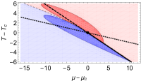
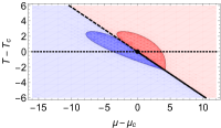
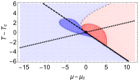
Figure 8: Contours of $\chi_{3}$ when the slope (90) of the $r=0$ line (dotted) is negative, zero and positive (from left to right). The contour $\chi_{3}=0$ is shown by the thin dashed line. The thick dashed line is the $h=0$ axis (crossover). The regions of negative $\chi_{3}$ are shown in red, and the regions of positive value of $\chi_{3}$ are in blue. Note that $\chi_{3}$ on the crossover line has the same sign as the slope of the $r=0$ line.

Appendix A The size of the critical region

Here we describe how the parameters of the mapping control the size of the critical region. We define the critical region as the region where the singular part of the equation of state dominates over the regular part. This comparison cannot be done on the pressure itself, since the critical contribution to pressure vanishes at the critical point (as $r^{2-\alpha}$). A reasonable measure of the critical region should be based on a quantity which is singular at the critical point, such as the baryon susceptibility, $\chi_{2}=P_{\mu\mu}$. We shall evaluate the size of the critical region along the crossover, $h=0$, line. The singular part of $\chi_{2}$ is given by, at $h=0$,

$$\chi_{2}^{\rm sing}\sim AG_{\mu\mu}(r,0)\sim AG_{hh}(r,0)h_{\mu}^{2}\sim Ar^{-\gamma}\left(\frac{s_{1}}{wT_{c}s_{12}}\right)^{2}\sim A\left(\frac{\Delta\mu}{\rho wT_{c}c_{1}}\right)^{-\gamma}\left(\frac{s_{1}}{wT_{c}s_{12}}\right)^{2}$$ (91)

where $s_{1}=\sin\alpha_{1},\,c_{1}=\cos\alpha_{1}$ and $s_{12}=\sin(\alpha_{1}-\alpha_{2})$. Comparing this to the regular contribution of order $\chi_{2}^{\rm reg}\sim T_{c}^{2}$, we find for the extent of the critical region in the $\mu$ direction:

$$\Delta\mu_{\rm CR}\sim T_{c}\rho wc_{1}\left(\frac{s_{1}\sqrt{A}}{wT_{c}^{2}s_{12}}\right)^{2/\gamma}$$ (92)

Therefore, while increasing parameters $\rho$ and $A$ increases the size of the critical region, the effect of increasing the parameter $w$ is the opposite: $\Delta\mu_{\rm CR}\sim w^{1-2/\gamma}$. In the mean-field theory $\gamma=1$ and $\Delta\mu_{\rm CR}$ is inversely proportional to $w$.

Appendix B Mapping parameters for the van der Waals equation of state

In this appendix, to illustrate the use of the formalism developed in Section III we shall derive the equations for the mapping parameters in the van der Waals equation of state. The well-known equation of state expresses pressure as a function of particle density $n$ and temperature $T$:

$$P=\frac{nT}{1-bn}-an^{2}\,,$$ (93)

where $a$ and $b$ are van der Waals constants corresponding to the strength of the particle attraction and the hard-core volume, respectively. The van der Waals equation of state possesses a critical point at

$$n_{c}=\frac{1}{3b},\quad T_{c}=\frac{8a}{27b},\quad P_{c}=\frac{a}{27b^{2}}\,.$$ (94)

The equation of state (93) can be expressed in the mean-field (Ginzburg-Landau) form

$$P(\mu,T)=-A\min_{n}\Omega(n,T,\mu)\,,$$ (95)

where

$$A\Omega(n,T,\mu)=\mu n-F(T,n)$$ (96)

is expressed in terms of the free energy $F(n,T)$, which is the Legendre transform of $P(\mu,T)$:

$$F(n,T) = n\mu(n,T)-P(\mu(n,T),T)\,.$$ (97)

In Eq. (97), but not in Eq. (96), the chemical potential $\mu(n,T)$ must be determined as a solution to $n=\partial P/\partial\mu$. This can be done by integrating the following set of partial differential equations:

$$\left(\frac{\partial\mu}{\partial n}\right)_{T} = \frac{1}{n}\left(\frac{\partial p}{\partial n}\right)_{T}\,;$$ (98)

$$\left(\frac{\partial\mu}{\partial T}\right)_{n} = \frac{1}{n}\left(\frac{\partial p}{\partial T}\right)_{n}-\frac{s}{n}\,;$$ (99)

$$\left(\frac{\partial s}{\partial T}\right)_{n} = \frac{c_{v}n}{T}\,,$$ (100)

where $c_{v}$ is the heat capacity per particle (e.g., $3/2$ for monoatomic gas). Using the values of $\mu$ and $s$ at the critical point, $\mu_{c}$ and $s_{c}$, as initial conditions one finds

$$\mu(n,T) = T\left(\log\frac{2bn}{1-bn}-\log\frac{2bn_{c}}{1-bn_{c}}\right)+\frac{T}{1-bn}-\frac{T_{c}}{1-bn_{c}}$$ (101)

$$-2a(n-n_{c})-c_{v}T\log\frac{T}{T_{c}}+\left(c_{v}-\frac{s_{c}}{n_{c}}\right)(T-T_{c})+\mu_{c}\,.$$

Expanding the potential $\Omega$ one obtains

$$A\Omega(n,T,\mu) = A\Omega(n_{c},T_{c},\mu_{c})-\left(\Delta\mu-\left(\frac{3}{2}-3bs_{c}\right)\Delta T\right)\eta+\frac{27b}{8}\Delta T\eta^{2}+\frac{9ab^{2}}{8}\eta^{4}-\frac{27ab^{3}}{40}\eta^{5}+\ldots\,,$$ (102)

where $\eta=n-n_{c}$, $\Delta T=T-T_{c}$ and $\Delta\mu=\mu-\mu_{c}$. Comparing to Eq. (23) we identify

$$A{\bar{h}} = \Delta\mu-\left(\frac{3}{2}-3bs_{c}\right)\Delta T,$$ (103)

$$A{\bar{r}} = \frac{27b}{4}\Delta T,$$ (104)

$$Au = \frac{9ab^{2}}{2},\quad v=-\frac{3b}{20}.$$ (105)

Using Eqs. (26), (27) one then finds

$$h = A^{-3/4}\left(\frac{9ab^{2}}{2}\right)^{-1/4}\left(\Delta\mu-\left(\frac{3}{2}-3bs_{c}\right)\Delta T\right)$$ (106)

$$r = -A^{-1/2}\frac{3}{10}\left(\frac{9a}{2}\right)^{-1/2}\left(\Delta\mu+3\left(b\,s_{c}-8\right)\Delta T\right)\,.$$ (107)

Using Eqs. (13), (14), (16) and (17) one finally obtains

$$\tan\alpha_{1} = -\left(\frac{3}{2}-\frac{s_{c}}{n_{c}}\right)^{-1}\,;$$ (108)

$$\tan\alpha_{2} = -\left(24-\frac{s_{c}}{n_{c}}\right)^{-1}\,;$$ (109)

$$\rho = 5\left(\frac{3P_{c}}{T_{c}^{4}}\right)^{1/4}\sqrt{\frac{4s_{c}\left(s_{c}-3n_{c}\right)+13n_{c}^{2}}{s_{c}\left(s_{c}-48n_{c}\right)+577n_{c}^{2}}}\,;$$ (110)

$$w = \frac{1}{40}\left(\frac{T_{c}^{4}}{3P_{c}}\right)^{3/4}\sqrt{\frac{s_{c}}{n_{c}}\left(\frac{s_{c}}{n_{c}}-48\right)+577}\,.$$ (111)

References

- (1) M. A. Stephanov, “QCD phase diagram and the critical point,” Prog. Theor. Phys. Suppl. 153 (2004) 139–156, arXiv:hep-ph/0402115 [hep-ph]. [Int. J. Mod. Phys.A20,4387(2005)].
- (2) X. Luo and N. Xu, “Search for the QCD Critical Point with Fluctuations of Conserved Quantities in Relativistic Heavy-Ion Collisions at RHIC : An Overview,” Nucl. Sci. Tech. 28 no. 8, (2017) 112, arXiv:1701.02105 [nucl-ex].
- (3) H.-T. Ding, F. Karsch, and S. Mukherjee, “Thermodynamics of strong-interaction matter from Lattice QCD,” Int. J. Mod. Phys. E24 no. 10, (2015) 1530007, arXiv:1504.05274 [hep-lat].
- (4) M. A. Stephanov, K. Rajagopal, and E. V. Shuryak, “Signatures of the tricritical point in QCD,” Phys. Rev. Lett. 81 (1998) 4816–4819, arXiv:hep-ph/9806219 [hep-ph].
- (5) K. Rajagopal and F. Wilczek, “Static and dynamic critical phenomena at a second order QCD phase transition,” Nucl. Phys. B399 (1993) 395–425, arXiv:hep-ph/9210253 [hep-ph].
- (6) S. Gavin, A. Gocksch, and R. D. Pisarski, “QCD and the chiral critical point,” Phys. Rev. D49 (1994) R3079–R3082, arXiv:hep-ph/9311350 [hep-ph].
- (7) B. Widom, “Equation of state in the neighborhood of the critical point,” The Journal of Chemical Physics 43 no. 11, (1965) 3898–3905.
- (8) J. J. Rehr and N. D. Mermin, “Revised Scaling Equation of State at the Liquid-Vapor Critical Point,” Phys. Rev. A8 (1973) 472–480.
- (9) F. Karsch, E. Laermann, and C. Schmidt, “The Chiral critical point in three-flavor QCD,” Phys. Lett. B520 (2001) 41–49, arXiv:hep-lat/0107020 [hep-lat].
- (10) Y. Hatta and T. Ikeda, “Universality, the QCD critical / tricritical point and the quark number susceptibility,” Phys. Rev. D67 (2003) 014028, arXiv:hep-ph/0210284 [hep-ph].
- (11) C. Nonaka and M. Asakawa, “Hydrodynamical evolution near the QCD critical end point,” Phys. Rev. C71 (2005) 044904, arXiv:nucl-th/0410078 [nucl-th].
- (12) M. Bluhm and B. Kampfer, “Quasi-particle perspective on critical end-point,” PoS CPOD2006 (2006) 004, arXiv:hep-ph/0611083 [hep-ph].
- (13) P. Parotto, M. Bluhm, D. Mroczek, M. Nahrgang, J. Noronha-Hostler, K. Rajagopal, C. Ratti, T. Schäfer, and M. Stephanov, “Lattice-QCD-based equation of state with a critical point,” arXiv:1805.05249 [hep-ph].
- (14) Y. Akamatsu, D. Teaney, F. Yan, and Y. Yin, “Transits of the QCD Critical Point,” arXiv:1811.05081 [nucl-th].
- (15) K. Rummukainen, M. Tsypin, K. Kajantie, M. Laine, and M. E. Shaposhnikov, “The Universality class of the electroweak theory,” Nucl. Phys. B532 (1998) 283–314, arXiv:hep-lat/9805013 [hep-lat].
- (16) T. D. Lee and C.-N. Yang, “Statistical theory of equations of state and phase transitions. 2. Lattice gas and Ising model,” Phys. Rev. 87 (1952) 410–419. [,157(1952)].
- (17) M. E. Fisher, “Yang-Lee edge singularity and field theory,” Phys. Rev. Lett. 40 (1978) 1610.
- (18) P. Fonseca and A. Zamolodchikov, “Ising field theory in a magnetic field: Analytic properties of the free energy,” arXiv:hep-th/0112167 [hep-th].
- (19) X. An, D. Mesterházy, and M. A. Stephanov, “On spinodal points and Lee-Yang edge singularities,” J. Stat. Mech. 1803 no. 3, (2018) 033207, arXiv:1707.06447 [hep-th].
- (20) A. M. Halasz, A. D. Jackson, R. E. Shrock, M. A. Stephanov, and J. J. M. Verbaarschot, “On the phase diagram of QCD,” Phys. Rev. D58 (1998) 096007, arXiv:hep-ph/9804290 [hep-ph].
- (21) D. J. Wallace and R. K. P. Zia, “Parametric models and the Ising equation of state at order ,” J. Phys. C 7 (1974) 3480.
- (22) I. D. Lawrie, “Tricritical scaling and renormalisation of 6operators in scalar systems near four dimensions,” Journal of Physics A: Mathematical and General 12 no. 6, (Jun, 1979) 919–940.
- (23) J. F. Nicoll, “Critical phenomena of fluids: Asymmetric Landau-Ginzburg-Wilson model,” Phys. Rev. A24 (1981) 2203–2220.
- (24) D. J. Amit, Field theory, the renormalization group, and critical phenomena. Singapore, World Scientific, 1984.
- (25) E. Brezin, D. J. Wallace, and K. G. Wilson, “Feynman graph expansion for the equation of state near the critical point (Ising-like case),” Phys. Rev. Lett. 29 (1972) 591–594.
- (26) R. Guida and J. Zinn-Justin, “Critical exponents of the N vector model,” J. Phys. A31 (1998) 8103–8121, arXiv:cond-mat/9803240 [cond-mat].
- (27) J. C. Le Guillou and J. Zinn-Justin, “Critical Exponents from Field Theory,” Phys. Rev. B21 (1980) 3976–3998.
- (28) A. Pelissetto and E. Vicari, “Critical phenomena and renormalization group theory,” Phys. Rept. 368 (2002) 549–727, arXiv:cond-mat/0012164 [cond-mat].
- (29) J. Zinn-Justin, “Quantum field theory and critical phenomena,” Int. Ser. Monogr. Phys. 77 (1989) 1–914.
- (30) K. E. Newman and E. K. Riedel, “Critical exponents by the scaling-field method: The isotropic N-vector model in three dimensions,” Phys. Rev. B30 (1984) 6615–6638.
- (31) D. F. Litim and D. Zappala, “Ising exponents from the functional renormalisation group,” Phys. Rev. D83 (2011) 085009, arXiv:1009.1948 [hep-th].
- (32) D. F. Litim and L. Vergara, “Subleading critical exponents from the renormalization group,” Phys. Lett. B581 (2004) 263–269, arXiv:hep-th/0310101 [hep-th].
- (33) STAR Collaboration, L. Adamczyk et al., “Energy Dependence of Moments of Net-proton Multiplicity Distributions at RHIC,” Phys. Rev. Lett. 112 (2014) 032302, arXiv:1309.5681 [nucl-ex].
- (34) STAR Collaboration, X. Luo, “Energy Dependence of Moments of Net-Proton and Net-Charge Multiplicity Distributions at STAR,” PoS CPOD2014 (2015) 019, arXiv:1503.02558 [nucl-ex].