Generalization Bounds of Stochastic Gradient Descent for Wide and Deep Neural Networks
Abstract
We study the training and generalization of deep neural networks (DNNs) in the over-parameterized regime, where the network width (i.e., number of hidden nodes per layer) is much larger than the number of training data points. We show that, the expected - loss of a wide enough ReLU network trained with stochastic gradient descent (SGD) and random initialization can be bounded by the training loss of a random feature model induced by the network gradient at initialization, which we call a neural tangent random feature (NTRF) model. For data distributions that can be classified by NTRF model with sufficiently small error, our result yields a generalization error bound in the order of that is independent of the network width. Our result is more general and sharper than many existing generalization error bounds for over-parameterized neural networks. In addition, we establish a strong connection between our generalization error bound and the neural tangent kernel (NTK) proposed in recent work.
1 Introduction
Deep learning has achieved great success in a wide range of applications including image processing (Krizhevsky et al., 2012), natural language processing (Hinton et al., 2012) and reinforcement learning (Silver et al., 2016). Most of the deep neural networks used in practice are highly over-parameterized, such that the number of parameters is much larger than the number of training data. One of the mysteries in deep learning is that, even in an over-parameterized regime, neural networks trained with stochastic gradient descent can still give small test error and do not overfit. In fact, a famous empirical study by Zhang et al. (2017) shows the following phenomena:
-
•
Even if one replaces the real labels of a training data set with purely random labels, an over-parameterized neural network can still fit the training data perfectly. However since the labels are independent of the input, the resulting neural network does not generalize to the test dataset.
-
•
If the same over-parameterized network is trained with real labels, it not only achieves small training loss, but also generalizes well to the test dataset.
While a series of recent work has theoretically shown that a sufficiently over-parameterized (i.e., sufficiently wide) neural network can fit random labels (Du et al., 2019b; Allen-Zhu et al., 2019b; Du et al., 2019a; Zou et al., 2019), the reason why it can generalize well when trained with real labels is less understood. Existing generalization bounds for deep neural networks (Neyshabur et al., 2015; Bartlett et al., 2017; Neyshabur et al., 2018; Golowich et al., 2018; Dziugaite and Roy, 2017; Arora et al., 2018; Li et al., 2018; Wei et al., 2019; Neyshabur et al., 2019) based on uniform convergence usually cannot provide non-vacuous bounds (Langford and Caruana, 2002; Dziugaite and Roy, 2017) in the over-parameterized regime. In fact, the empirical observation by Zhang et al. (2017) indicates that in order to understand deep learning, it is important to distinguish the true data labels from random labels when studying generalization. In other words, it is essential to quantify the “classifiability” of the underlying data distribution, i.e., how difficult it can be classified.
Certain effort has been made to take the “classifiability” of the data distribution into account for generalization analysis of neural networks. Brutzkus et al. (2018) showed that stochastic gradient descent (SGD) can learn an over-parameterized two-layer neural network with good generalization for linearly separable data. Li and Liang (2018) proved that, if the data satisfy certain structural assumption, SGD can learn an over-parameterized two-layer network with fixed second layer weights and achieve a small generalization error. Allen-Zhu et al. (2019a) studied the generalization performance of SGD and its variants for learning two-layer and three-layer networks, and used the risk of smaller two-layer or three-layer networks with smooth activation functions to characterize the classifiability of the data distribution. There is another line of studies on the algorithm-dependent generalization bounds of neural networks in the over-parameterized regime (Daniely, 2017; Arora et al., 2019a; Cao and Gu, 2020; Yehudai and Shamir, 2019; E et al., 2019), which quantifies the classifiability of the data with a reference function class defined by random features (Rahimi and Recht, 2008, 2009) or kernels111Since random feature models and kernel methods are highly related (Rahimi and Recht, 2008, 2009), we group them into the same category. More details are discussed in Section 3.2.. Specifically, Daniely (2017) showed that a neural network of large enough size is competitive with the best function in the conjugate kernel class of the network. Arora et al. (2019a) gave a generalization error bound for two-layer ReLU networks with fixed second layer weights based on a ReLU kernel function. Cao and Gu (2020) showed that deep ReLU networks trained with gradient descent can achieve small generalization error if the data can be separated by certain random feature model (Rahimi and Recht, 2009) with a margin. Yehudai and Shamir (2019) used the expected loss of a similar random feature model to quantify the generalization error of two-layer neural networks with smooth activation functions. A similar generalization error bound was also given by E et al. (2019), where the authors studied the optimization and generalization of two-layer networks trained with gradient descent. However, all the aforementioned results are still far from satisfactory: they are either limited to two-layer networks, or restricted to very simple and special reference function classes.
In this paper, we aim at providing a sharper and generic analysis on the generalization of deep ReLU networks trained by SGD. In detail, we base our analysis upon the key observations that near random initialization, the neural network function is almost a linear function of its parameters and the loss function is locally almost convex. This enables us to prove a cumulative loss bound of SGD, which further leads to a generalization bound by online-to-batch conversion (Cesa-Bianchi et al., 2004). The main contributions of our work are summarized as follows:
-
•
We give a bound on the expected - error of deep ReLU networks trained by SGD with random initialization. Our result relates the generalization bound of an over-parameterized ReLU network with a random feature model defined by the network gradients, which we call neural tangent random feature (NTRF) model. It also suggests an algorithm-dependent generalization error bound of order , which is independent of network width, if the data can be classified by the NTRF model with small enough error.
-
•
Our analysis is general enough to cover recent generalization error bounds for neural networks with random feature based reference function classes, and provides better bounds. Our expected - error bound directly covers the result by Cao and Gu (2020), and gives a tighter sample complexity when reduced to their setting, i.e., versus where is the target generalization error. Compared with recent results by Yehudai and Shamir (2019); E et al. (2019) who only studied two-layer networks, our bound not only works for deep networks, but also uses a larger reference function class when reduced to the two-layer setting, and therefore is sharper.
-
•
Our result has a direct connection to the neural tangent kernel studied in Jacot et al. (2018). When interpreted in the language of kernel method, our result gives a generalization bound in the form of , where is the training label vector, and is the neural tangent kernel matrix defined on the training input data. This form of generalization bound is similar to, but more general and tighter than the bound given by Arora et al. (2019a).
Notation We use lower case, lower case bold face, and upper case bold face letters to denote scalars, vectors and matrices respectively. For a vector and a number , let . We also define . For a matrix , we use to denote the number of non-zero entries of , and denote and for . For two matrices , we define . We denote by if is positive semidefinite. In addition, we define the asymptotic notations , , and as follows. Suppose that and be two sequences. We write if , and if . We use and to hide the logarithmic factors in and .
2 Problem Setup
In this section we introduce the basic problem setup. Following the same standard setup implemented in the line of recent work (Allen-Zhu et al., 2019b; Du et al., 2019a; Zou et al., 2019; Cao and Gu, 2020), we consider fully connected neural networks with width , depth and input dimension . Such a network is defined by its weight matrices at each layer: for , let , , and be the weight matrices of the network. Then the neural network with input is defined as
| (2.1) |
where is the entry-wise activation function. In this paper, we only consider the ReLU activation function , which is the most commonly used activation function in applications. It is also arguably one of the most difficult activation functions to analyze, due to its non-smoothess. We remark that our result can be generalized to many other Lipschitz continuous and smooth activation functions. For simplicity, we follow Allen-Zhu et al. (2019b); Du et al. (2019a) and assume that the widths of each hidden layer are the same. Our result can be easily extended to the setting that the widths of each layer are not equal but in the same order, as discussed in Zou et al. (2019); Cao and Gu (2020).
When , the neural network reduces to a linear function, which has been well-studied. Therefore, for notational simplicity we focus on the case , where the parameter space is defined as
We also use to denote the collection of weight matrices for all layers. For , we define their inner product as .
The goal of neural network learning is to minimize the expected risk, i.e.,
| (2.2) |
where is the loss defined on any example , and is the loss function. Without loss of generality, we consider the cross-entropy loss in this paper, which is defined as . We would like to emphasize that our results also hold for most convex and Lipschitz continuous loss functions such as hinge loss. We now introduce stochastic gradient descent based training algorithm for minimizing the expected risk in (2.2). The detailed algorithm is given in Algorithm 1.
The initialization scheme for given in Algorithm 1 generates each entry of the weight matrices from a zero-mean independent Gaussian distribution, whose variance is determined by the rule that the expected length of the output vector in each hidden layer is equal to the length of the input. This initialization method is also known as He initialization (He et al., 2015). Here the last layer parameter is initialized with variance instead of since the last layer is not associated with the ReLU activation function.
3 Main Results
In this section we present the main results of this paper. In Section 3.1 we give an expected - error bound against a neural tangent random feature reference function class. In Section 3.2, we discuss the connection between our result and the neural tangent kernel proposed in Jacot et al. (2018).
3.1 An Expected - Error Bound
In this section we give a bound on the expected - error obtained by Algorithm 1. Our result is based on the following assumption.
Assumption 3.1.
The data inputs are normalized: for all .
Assumption 3.1 is a standard assumption made in almost all previous work on optimization and generalization of over-parameterized neural networks (Du et al., 2019b; Allen-Zhu et al., 2019b; Du et al., 2019a; Zou et al., 2019; Oymak and Soltanolkotabi, 2019; E et al., 2019). As is mentioned in Cao and Gu (2020), this assumption can be relaxed to for all , where are absolute constants.
For any , we define its -neighborhood as
Below we introduce the neural tangent random feature function class, which serves as a reference function class to measure the “classifiability” of the data, i.e., how easy it can be classified.
Definition 3.2 (Neural Tangent Random Feature).
Let be generated via the initialization scheme in Algorithm 1. The neural tangent random feature (NTRF) function class is defined as
where measures the size of the function class, and is the width of the neural network.
The name “neural tangent random feature” is inspired by the neural tangent kernel proposed by Jacot et al. (2018), because the random features are the gradients of the neural network with random weights. Connections between the neural tangent random features and the neural tangent kernel will be discussed in Section 3.2.
We are ready to present our main result on the expected - error bound of Algorithm 1.
Theorem 3.3.
For any and , there exists
such that if , then with probability at least over the randomness of , the output of Algorithm 1 with step size for some small enough absolute constant satisfies
| (3.1) |
where the expectation is taken over the uniform draw of from .
The expected - error bound given by Theorem 3.3 consists of two terms: The first term in (3.1) relates the expected - error achieved by Algorithm 1 with a reference function class–the NTRF function class in Definition 3.2. The second term in (3.1) is a standard large-deviation error term. As long as , this term matches the standard rate in PAC learning bounds (Shalev-Shwartz and Ben-David, 2014).
Remark 3.4.
The parameter in Theorem 3.3 is from the NTRF class and introduces a trade-off in the bound: when is small, the corresponding NTRF class is small, making the first term in (3.1) large, and the second term in (3.1) is small. When is large, the corresponding function class is large, so the first term in (3.1) is small, and the second term will be large. In particular, if we set , the second term in (3.1) will be . In this case, the “classifiability” of the underlying data distribution is determined by how well its i.i.d. samples can be classified by . In other words, Theorem 3.3 suggests that if the data can be classified by a function in the NTRF function class with a small training error, the over-parameterized ReLU network learnt by Algorithm 1 will have a small generalization error.
Remark 3.5.
The expected - error bound given by Theorem 3.3 is in a very general form. It directly covers the result given by Cao and Gu (2020). In Appendix A.1, we show that under the same assumptions made in Cao and Gu (2020), to achieve expected - error, our result requires a sample complexity of order , which outperforms the result in Cao and Gu (2020) by a factor of .
Remark 3.6.
Our generalization bound can also be compared with two recent results (Yehudai and Shamir, 2019; E et al., 2019) for two-layer neural networks. When , the NTRF function class can be written as
In contrast, the reference function classes studied by Yehudai and Shamir (2019) and E et al. (2019) are contained in the following random feature class:
where are the random weights generated by the initialization schemes in Yehudai and Shamir (2019); E et al. (2019)222Normalizing weights to the same scale is necessary for a proper comparison. See Appendix A.2 for details.. Evidently, our NTRF function class is richer than –it also contains the features corresponding to the first layer gradient of the network at random initialization, i.e., . As a result, our generalization bound is sharper than those in Yehudai and Shamir (2019); E et al. (2019) in the sense that we can show that neural networks trained with SGD can compete with the best function in a larger reference function class.
As previously mentioned, the result of Theorem 3.3 can be easily extended to the setting where the widths of different layers are different. We should expect that the result remains almost the same, except that we assume the widths of hidden layers are all larger than or equal to . We would also like to point out that although this paper considers the cross-entropy loss, the proof of Theorem 3.3 offers a general framework based on the fact that near initialization, the neural network function is almost linear in terms of its weights. We believe that this proof framework can potentially be applied to most practically useful loss functions: whenever is convex/Lipschitz continuous/smooth, near initialization, is also almost convex/Lipschitz continuous/smooth in for all , and therefore standard online optimization analysis can be invoked with online-to-batch conversion to provide a generalization bound. We refer to Section 4 for more details.
3.2 Connection to Neural Tangent Kernel
Besides quantifying the classifiability of the data with the NTRF function class , an alternative way to apply Theorem 3.3 is to check how large the parameter needs to be in order to make the first term in (3.1) small enough (e.g., smaller than ). In this subsection, we show that this type of analysis connects Theorem 3.3 to the neural tangent kernel proposed in Jacot et al. (2018) and later studied by Yang (2019); Lee et al. (2019); Arora et al. (2019b). Specifically, we provide an expected - error bound in terms of the neural tangent kernel matrix defined over the training data. We first define the neural tangent kernel matrix for the neural network function in (2.1).
Definition 3.7 (Neural Tangent Kernel Matrix).
For any , define
Then we call the neural tangent kernel matrix of an -layer ReLU network on training inputs .
Definition 3.7 is the same as the original definition in Jacot et al. (2018) when restricting the kernel function on , except that there is an extra coefficient in the second and third lines. This extra factor is due to the difference in initialization schemes–in our paper the entries of hidden layer matrices are randomly generated with variance , while in Jacot et al. (2018) the variance of the random initialization is . We remark that this extra factor in Definition 3.7 will remove the exponential dependence on the network depth in the kernel matrix, which is appealing. In fact, it is easy to check that under our scaling, the diagonal entries of are all ’s, and the diagonal entries of are all ’s.
The following lemma is a summary of Theorem 1 and Proposition 2 in Jacot et al. (2018), which ensures that is the infinite-width limit of the Gram matrix , and is positive-definite as long as no two training inputs are parallel.
Lemma 3.8 (Jacot et al. (2018)).
For an layer ReLU network with parameter set initialized in Algorithm 1, as the network width 333The original result by Jacot et al. (2018) requires that the widths of different layers go to infinity sequentially. Their result was later improved by Yang (2019) such that the widths of different layers can go to infinity simultaneously., it holds that
where the expectation is taken over the randomness of . Moreover, as long as each pair of inputs among are not parallel, is positive-definite.
Remark 3.9.
Lemmas 3.8 clearly shows the difference between our neural tangent kernel matrix in Definition 3.7 and the Gram matrix defined in Definition 5.1 in Du et al. (2019a). For any , by Lemma 3.8 we have
In contrast, the corresponding entry in is
It can be seen that our definition of kernel matrix takes all layers into consideration, while Du et al. (2019a) only considered the last hidden layer (i.e., second last layer). Moreover, it is clear that . Since the smallest eigenvalue of the kernel matrix plays a key role in the analysis of optimization and generalization of over-parameterized neural networks (Du et al., 2019b, a; Arora et al., 2019a), our neural tangent kernel matrix can potentially lead to better bounds than the Gram matrix studied in Du et al. (2019a).
Corollary 3.10.
Let and . For any , there exists that only depends on and such that if , then with probability at least over the randomness of , the output of Algorithm 1 with step size for some small enough absolute constant satisfies
where the expectation is taken over the uniform draw of from .
Apparently, by choosing in Corollary 3.10, one can also obtain a bound on the expected error of the form .
Remark 3.11.
Corollary 3.10 gives an algorithm-dependent generalization error bound of over-parameterized -layer neural networks trained with SGD. It is worth noting that recently Arora et al. (2019a) gives a generalization bound for two-layer networks with fixed second layer weights, where is defined as
Our result in Corollary 3.10 can be specialized to two-layer neural networks by choosing , and yields a bound , where
Here the extra term corresponds to the training of the second layer–it is the limit of . Since we have , our bound is sharper than theirs. This comparison also shows that, our result generalizes the result in Arora et al. (2019a) from two-layer, fixed second layer networks to deep networks with all parameters being trained.
Remark 3.12.
Corollary 3.10 is based on the asymptotic convergence result in Lemma 3.8, which does not show how wide the network need to be in order to make the Gram matrix close enough to the NTK matrix. Very recently, Arora et al. (2019b) provided a non-asymptotic convergence result for the Gram matrix, and showed the equivalence between an infinitely wide network trained by gradient flow and a kernel regression predictor using neural tangent kernel, which suggests that the generalization of deep neural networks trained by gradient flow can potentially be measured by the corresponding NTK. Utilizing this non-asymptotic convergence result, one can potentially specify the detailed dependency of on , , and in Corollary 3.10.
Remark 3.13.
Corollary 3.10 demonstrates that the generalization bound given by Theorem 3.3 does not increase with network width , as long as is large enough. Moreover, it provides a clear characterization of the classifiability of data. In fact, the factor in the generalization bound given in Corollary 3.10 is exactly the NTK-induced RKHS norm of the kernel regression classifier on data . Therefore, if for some with bounded norm in the NTK-induced reproducing kernel Hilbert space (RKHS), then over-parameterized neural networks trained with SGD generalize well. In Appendix E, we provide some numerical evaluation of the leading terms in the generalization bounds in Theorem 3.3 and Corollary 3.10 to demonstrate that they are very informative on real-world datasets.
4 Proof of Main Theory
In this section we provide the proof of Theorem 3.3 and Corollary 3.10, and explain the intuition behind the proof. For notational simplicity, for we denote .
4.1 Proof of Theorem 3.3
Before giving the proof of Theorem 3.3, we first introduce several lemmas. The following lemma states that near initialization, the neural network function is almost linear in terms of its weights.
Lemma 4.1.
There exists an absolute constant such that, with probability at least over the randomness of , for all and with , it holds uniformly that
Since the cross-entropy loss is convex, given Lemma 4.1, we can show in the following lemma that near initialization, is also almost a convex function of for any .
Lemma 4.2.
There exists an absolute constant such that, with probability at least over the randomness of , for any , and with , it holds uniformly that
The locally almost convex property of the loss function given by Lemma 4.2 implies that the dynamics of Algorithm 1 is similar to the dynamics of convex optimization. We can therefore derive a bound of the cumulative loss. The result is given in the following lemma.
Lemma 4.3.
For any , there exists
such that if , then with probability at least over the randomness of , for any , Algorithm 1 with , for some small enough absolute constant has the following cumulative loss bound:
We now finalize the proof by applying an online-to-batch conversion argument (Cesa-Bianchi et al., 2004), and use Lemma 4.1 to relate the neural network function with a function in the NTRF function class.
Proof of Theorem 3.3.
For , let . Since cross-entropy loss satisfies , we have . Therefore, setting in Lemma 4.3 gives that, if is set as , then with probability at least ,
| (4.1) |
Note that for any , only depends on and is independent of . Therefore by Proposition 1 in Cesa-Bianchi et al. (2004), with probability at least we have
| (4.2) |
By definition, we have . Therefore combining (4.1) and (4.2) and applying union bound, we obtain that with probability at least ,
| (4.3) |
for all . We now compare the neural network function with the function . We have
where the first inequality is by the -Lipschitz continuity of and Lemma 4.1, the second inequality is by , and last inequality holds as long as for some large enough absolute constant . Plugging the inequality above into (4.3) gives
Taking infimum over and rescaling finishes the proof. ∎
4.2 Proof of Corollary 3.10
In this subsection we prove Corollary 3.10. The following lemma shows that at initialization, with high probability, the neural network function value at all the training inputs are of order .
Lemma 4.4.
For any , if for a large enough absolute constant , then with probability at least , for all .
We now present the proof of Corollary 3.10. The idea is to construct suitable target values , and then bound the norm of the solution of the linear equations , . In specific, for any with , we examine the minimum distance solution to that fit the data well and use it to construct a specific function in .
Proof of Corollary 3.10.
Set , then for cross-entropy loss we have for . Moreover, let . Then by Lemma 4.4, with probability at least , for all . For any with , let and , then it holds that for any ,
and therefore
| (4.4) |
Denote . Note that entries of are all bounded by . Therefore, the largest eigenvalue of is at most , and we have . By Lemma 3.8 and standard matrix perturbation bound, there exists such that, if , then with probability at least , is strictly positive-definite and
| (4.5) |
Let be the singular value decomposition of , where have orthogonal columns, and is a diagonal matrix. Let , then we have
| (4.6) |
Moreover, by direct calculation we have
Therefore by (4.5) and the fact that , we have
Let be the parameter collection reshaped from . Then clearly
and therefore . Moreover, by (4.6), we have . Plugging this into (4.4) then gives
Since , applying Theorem 3.3 and taking infimum over completes the proof. ∎
5 Conclusions and Future Work
In this paper we provide an expected - error bound for wide and deep ReLU networks trained with SGD. This generalization error bound is measured by the NTRF function class. The connection to the neural tangent kernel function studied in Jacot et al. (2018) is also discussed. Our result covers a series of recent generalization bounds for wide enough neural networks, and provides better bounds.
An important future work is to improve the over-parameterization condition in Theorem 3.3 and Corollary 3.10. Other future directions include proving sample complexity lower bounds in the over-parameterized regime, implementing the results in Jain et al. (2019) to obtain last iterate bound of SGD, and establishing uniform convergence based generalization bounds for over-parameterized neural networks with methods developped in Bartlett et al. (2017); Neyshabur et al. (2018); Long and Sedghi (2019).
Acknowledgement
We would like to thank Peter Bartlett for a valuable discussion, and Simon S. Du for pointing out a related work (Arora et al., 2019b). We also thank the anonymous reviewers and area chair for their helpful comments. This research was sponsored in part by the National Science Foundation CAREER Award IIS-1906169, IIS-1903202, and Salesforce Deep Learning Research Award. The views and conclusions contained in this paper are those of the authors and should not be interpreted as representing any funding agencies.
Appendix A Comparison with Recent Results
In this section we compare our result in Theorem 3.3 with recent generalization error bounds for over-paramerized neural networks by Cao and Gu (2020); Yehudai and Shamir (2019); E et al. (2019), and backup our discussions in Remark 3.5 and Remark 3.6.
A.1 Comparison with Cao and Gu (2020)
In this section we provide direct comparison between our result in Theorem 3.3 and Theorem 4.4 in Cao and Gu (2020). To concretely compare these two results, we apply our result to the setting studied in Cao and Gu (2020), which is based on the following assumption.
Assumption A.1.
There exist a constant and
where the density of standard Gaussian vectors, such that for all .
Under Assumption 3.1 and Assumption A.1, in order to train the network to achieve expected - loss, Cao and Gu (2020) gave a sample complexity of order . In comparison, our result in Theorem 3.3 leads to the following corollary.
Corollary A.2.
Under Assumption 3.1 and Assumption A.1, for any , there exists
such that if , then with probability at least over the randomness of , the parameters given by Algorithm 1 with for some small enough absolute constant satisfies
where the expectation is taken over the draws of training examples as well as the uniform draw of from .
By setting the expected - loss bound to , we obtain a sample complexity of order , which is better than the sample complexity given in Cao and Gu (2020) by a factor of .
A.2 Comparison with Yehudai and Shamir (2019); E et al. (2019)
Here we give a detailed explanation to Remark 3.6, where we compare our result with Yehudai and Shamir (2019); E et al. (2019). The reference function classes studied in these two papers share the same general form:
where is a constant, and is the first layer parameter matrix whose rows are sampled from certain distribution associated to the initialization scheme. Specifically, Yehudai and Shamir (2019) studied the case where is the uniform distribution over the -dimensional cube , while E et al. (2019) studied the uniform distribution over the sphere . By standard concentration inequality, we can see that in both papers, with high probability, the distribution gives with . In terms of second layer initialization , the generalization results in both papers require that . With such a scaling, we can apply the following lemma.
Lemma A.3.
Suppose that be weights satisfying for some , then
where
and is the activation function of interest.
We compare our result with the bounds given by Yehudai and Shamir (2019); E et al. (2019) by comparing the reference function classes we use. Apparently, a larger reference function class in general gives a better generalization error bound. Such a comparison requires us to adjust the scaling of initialized parameters. Based on our previous discussion, it is easy to see that the initialized second layer weights in our work and Yehudai and Shamir (2019); E et al. (2019) are all of the same scaling. However, the of first layer weight matrix in Yehudai and Shamir (2019); E et al. (2019) is larger than ours by a factor of . Adjusting this scaling difference will give an extra factor , which matches the factor in the definition of our neural network function. Note that even after adjusting the scaling of parameters, these random feature function classes are not directly comparable, since the activation functions and the distributions of random weights are different. However, an informal comparison can already clearly show the advantage of our result. Moreover, we remark that at least for two-layer networks, our analysis can be easily generalized to other activation functions and initialization methods, and the resulting NTRF class should be strictly larger than the random feature function classes used in Yehudai and Shamir (2019); E et al. (2019). This justifies our discussion in Remark 3.6.
Appendix B Proofs of Technical Lemmas in Section 4
In this section we provide the proofs of the technical lemmas in Section 4. We first introduce some extra notations. Following Allen-Zhu et al. (2019b), for a parameter collection and , we denote
as the hidden layer outputs of the network. We also define binary diagonal matrices
For and , we use , and , to denote the hidden layer outputs and binary diagonal matrices with parameter collections and respectively. We also implement the following matrix product notation which is also used in Zou et al. (2019); Cao and Gu (2020):
With this notation, we have the following matrix product representation of the neural network gradients:
B.1 Proof of Lemma 4.1
The following two lemmas are proved based on several results given by Allen-Zhu et al. (2019b). Note that in their paper, both the first and the last layers of the network are fixed, which is slightly different from our setting. We remark that this difference does not affect the result.
Lemma B.1.
If , then with probability at least , for all , and .
Lemma B.2.
If , then with probability at least , uniformly over:
-
•
any ,
-
•
any diagonal matrices with at most non-zero entries,
the following results hold:
-
(i)
For all , .
-
(ii)
For all , .
-
(iii)
For all ,
We are now ready to prove Lemma 4.1.
Proof of Lemma 4.1.
Since , , by direct calculation, we have
By Claim 8.2 in Allen-Zhu et al. (2019b) , there exist diagonal matrices with entries in such that and
for all . Therefore
By (iii) in Lemma B.2, with probability at least , we have
where the last inequality follows by Lemma B.1. This inequality finishes the proof. ∎
B.2 Proof of Lemma 4.2
Intuitively, Lemma 4.2 follows by the fact that the composition of a convex function and an almost linear function is almost convex. The detailed proof is as follows.
B.3 Proof of Lemma 4.3
To prove Lemma 4.3, we first introduce the following lemma which provides an upper bound for the gradient of the neural network function near initialization.
Lemma B.3.
There exists an absolute constant such that, with probability at least , for all , and with , it holds uniformly that
We now provide the final proof of Lemma 4.3.
Proof of Lemma 4.3.
Let , where is a small enough absolute constant such that the conditions on given in Lemmas 4.2 and B.3 hold. It is easy to see that as long as , we have . We now show that under our parameter choice, are inside as well.
This result follows by simple induction. Clearly we have . Suppose that . Then by Lemma B.3, for we have . Therefore
Plugging in our parameter choice , for some small enough absolute constant gives
where the last inequality holds as long as for some large enough constant . Therefore by induction we see that . As a result, the conditions of Lemmas 4.2 and B.3 are satisfied for and .
In the following, we utilize the results of Lemmas 4.2 and B.3 to prove the bound of cumulative loss. First of all, by Lemma 4.2, we have
Note that for the matrix inner product we have the equality . Applying this equality to the right hand side above gives
By Lemma B.3, for we have . Therefore
Telescoping over , we obtain
where in the first inequality we simply remove the term to obtain an upper bound, and the second inequality follows by the assumption that . Plugging in the parameter choice , for some small enough absolute constant gives
which finishes the proof. ∎
B.4 Proof of Lemma 4.4
Here we prove Lemma 4.4. The proof essentially follows by standard Gaussian tail bound and a bound on the length of last hidden layer output vector.
Appendix C Proofs of Results in Section A
C.1 Proof of Corollary A.2
The following lemma is a simplified version of Lemma C.2 in Cao and Gu (2020). Since the proof is almost the same as the proof of Lemma C.2 in Cao and Gu (2020), except replacing the -net argument with a simple union bound over training examples, we omit the proof detail here.
Lemma C.1.
For any , if for some large enough absolute constant , then with probability at least , there exists such that for all .
C.2 Proof of Lemma A.3
Here we give the proof of Lemma A.3. It is based on a simple construction.
Proof of Lemma A.3.
For any with , by the assumption that for some , we have satisfies . Therefore
This finishes the proof. ∎
Appendix D Proofs of Lemmas in Section B
D.1 Proof of Lemma B.1
D.2 Proof of Lemma B.2
We first introduce the following lemma characterizing the activation changes between networks with two close enough parameter sets and . This lemma directly follows by Lemma 8.2 in Allen-Zhu et al. (2019b) and triangle inequality.
Lemma D.1.
If , then with probability at least ,
for all , and .
Proof of Lemma B.2.
By Lemma D.1, with probability at least , for all and . Therefore we have for all and . Therefore by Lemma 5.6 in Allen-Zhu et al. (2019b), with probability at least we have . This completes the proof of (i) in Lemma B.2.
Similarly, to prove (iii), applying Lemma D.1 to gives that with probability at least , for all and . Now by Lemma 5.7 in Allen-Zhu et al. (2019b)444Note that is a random vector following the Gaussian distribution , which matches the distribution of the last layer parameters in Allen-Zhu et al. (2019b) for the binary classification case, where the output dimension of the network is . with to and , we have
| (D.1) | |||
| (D.2) |
Moreover, by result (i), we have
| (D.3) | |||
| (D.4) |
Combining equations (D.1), (D.2), (D.3), (D.4) and applying triangle inequality gives the desired final result (iii).
D.3 Proof of Lemma B.3
Appendix E Experimental Results
In this section we provide numerical calculations of the generalization bounds given by Theorem 3.3 and Corollary 3.10 on the MNIST dataset (LeCun et al., 1998). The main goal of these calculations is to demonstrate that the bounds given in our results are informative and can provide practical insight.
We have done experiments of a five-layer fully connected NN on MNIST dataset (3 versus 8), and calculated the first terms in the bounds given by Theorem 3.3 and Corollary 3.10.
- •
-
•
To demonstrate the scaling of the bound in Corollary 3.10, we calculate the value of , where is the true label vector with random flips. We plot in Figure 1 by varying the level of label noise, i.e., ratio of the labels that are flipped. Note that to simplify calculation, we do not consider the introduced in Corollary 3.10. Clearly, our calculation here gives an upper bound of the generalization bound in Corollary 3.10.
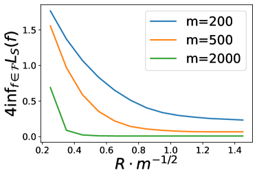
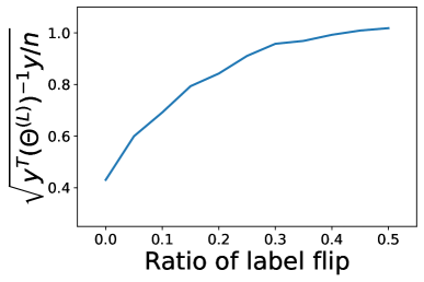
We can see that our bounds in both Theorem 3.3 and Corollary 3.10 give small and meaningful values. Moreover, these experimental results also back up our theoretical analysis. In Figure 1, the curves corresponding to different ’s also validate our theoretical result that the wider the network is, the shorter SGD needs to travel to fit the training data. In addition, the larger the size of reference function class (i.e., ), the smaller will be. In Figure 1, we can see that the noisier the labels, the larger the term is. When most of the labels are true labels, our bound can predict good test error; when the labels are purely random (i.e., ratio of label flip ), the bound on the test error can be larger than one. To sum up, these numerical results demonstrate the practical values of our generalization bounds, and suggest that our bounds can provide good measurements of the data classifiability.
References
- Allen-Zhu et al. (2019a) Allen-Zhu, Z., Li, Y. and Liang, Y. (2019a). Learning and generalization in overparameterized neural networks, going beyond two layers. In Advances in Neural Information Processing Systems.
- Allen-Zhu et al. (2019b) Allen-Zhu, Z., Li, Y. and Song, Z. (2019b). A convergence theory for deep learning via over-parameterization. In International Conference on Machine Learning.
- Arora et al. (2019a) Arora, S., Du, S., Hu, W., Li, Z. and Wang, R. (2019a). Fine-grained analysis of optimization and generalization for overparameterized two-layer neural networks. In International Conference on Machine Learning.
- Arora et al. (2019b) Arora, S., Du, S. S., Hu, W., Li, Z., Salakhutdinov, R. and Wang, R. (2019b). On exact computation with an infinitely wide neural net. In Advances in Neural Information Processing Systems.
- Arora et al. (2018) Arora, S., Ge, R., Neyshabur, B. and Zhang, Y. (2018). Stronger generalization bounds for deep nets via a compression approach. In International Conference on Machine Learning.
- Bartlett et al. (2017) Bartlett, P. L., Foster, D. J. and Telgarsky, M. J. (2017). Spectrally-normalized margin bounds for neural networks. In Advances in Neural Information Processing Systems.
- Brutzkus et al. (2018) Brutzkus, A., Globerson, A., Malach, E. and Shalev-Shwartz, S. (2018). Sgd learns over-parameterized networks that provably generalize on linearly separable data. In International Conference on Learning Representations.
- Cao and Gu (2020) Cao, Y. and Gu, Q. (2020). Generalization error bounds of gradient descent for learning over-parameterized deep relu networks. In the Thirty-Fourth AAAI Conference on Artificial Intelligence.
- Cesa-Bianchi et al. (2004) Cesa-Bianchi, N., Conconi, A. and Gentile, C. (2004). On the generalization ability of on-line learning algorithms. IEEE Transactions on Information Theory 50 2050–2057.
- Daniely (2017) Daniely, A. (2017). Sgd learns the conjugate kernel class of the network. In Advances in Neural Information Processing Systems.
- Du et al. (2019a) Du, S., Lee, J., Li, H., Wang, L. and Zhai, X. (2019a). Gradient descent finds global minima of deep neural networks. In International Conference on Machine Learning.
- Du et al. (2019b) Du, S. S., Zhai, X., Poczos, B. and Singh, A. (2019b). Gradient descent provably optimizes over-parameterized neural networks. In International Conference on Learning Representations.
- Dziugaite and Roy (2017) Dziugaite, G. K. and Roy, D. M. (2017). Computing nonvacuous generalization bounds for deep (stochastic) neural networks with many more parameters than training data. In Uncertainty in Artificial Intelligence.
- E et al. (2019) E, W., Ma, C., Wu, L. et al. (2019). A comparative analysis of the optimization and generalization property of two-layer neural network and random feature models under gradient descent dynamics. arXiv preprint arXiv:1904.04326 .
- Golowich et al. (2018) Golowich, N., Rakhlin, A. and Shamir, O. (2018). Size-independent sample complexity of neural networks. In Conference On Learning Theory.
- He et al. (2015) He, K., Zhang, X., Ren, S. and Sun, J. (2015). Delving deep into rectifiers: Surpassing human-level performance on imagenet classification. In Proceedings of the IEEE international conference on computer vision.
- Hinton et al. (2012) Hinton, G., Deng, L., Yu, D., Dahl, G. E., Mohamed, A.-r., Jaitly, N., Senior, A., Vanhoucke, V., Nguyen, P., Sainath, T. N. et al. (2012). Deep neural networks for acoustic modeling in speech recognition: The shared views of four research groups. IEEE Signal Processing Magazine 29 82–97.
- Jacot et al. (2018) Jacot, A., Gabriel, F. and Hongler, C. (2018). Neural tangent kernel: Convergence and generalization in neural networks. In Advances in neural information processing systems.
- Jain et al. (2019) Jain, P., Nagaraj, D. and Netrapalli, P. (2019). Making the last iterate of sgd information theoretically optimal. In Conference on Learning Theory.
- Krizhevsky et al. (2012) Krizhevsky, A., Sutskever, I. and Hinton, G. E. (2012). Imagenet classification with deep convolutional neural networks. In Advances in neural information processing systems.
- Langford and Caruana (2002) Langford, J. and Caruana, R. (2002). (not) bounding the true error. In Advances in Neural Information Processing Systems.
- LeCun et al. (1998) LeCun, Y., Bottou, L., Bengio, Y., Haffner, P. et al. (1998). Gradient-based learning applied to document recognition. Proceedings of the IEEE 86 2278–2324.
- Lee et al. (2019) Lee, J., Xiao, L., Schoenholz, S. S., Bahri, Y., Sohl-Dickstein, J. and Pennington, J. (2019). Wide neural networks of any depth evolve as linear models under gradient descent. arXiv preprint arXiv:1902.06720 .
- Li et al. (2018) Li, X., Lu, J., Wang, Z., Haupt, J. and Zhao, T. (2018). On tighter generalization bound for deep neural networks: Cnns, resnets, and beyond. arXiv preprint arXiv:1806.05159 .
- Li and Liang (2018) Li, Y. and Liang, Y. (2018). Learning overparameterized neural networks via stochastic gradient descent on structured data. In Advances in Neural Information Processing Systems.
- Long and Sedghi (2019) Long, P. M. and Sedghi, H. (2019). Size-free generalization bounds for convolutional neural networks. arXiv preprint arXiv:1905.12600 .
- Neyshabur et al. (2018) Neyshabur, B., Bhojanapalli, S., McAllester, D. and Srebro, N. (2018). A pac-bayesian approach to spectrally-normalized margin bounds for neural networks. In International Conference on Learning Representation.
- Neyshabur et al. (2019) Neyshabur, B., Li, Z., Bhojanapalli, S., LeCun, Y. and Srebro, N. (2019). Towards understanding the role of over-parametrization in generalization of neural networks. In International Conference on Learning Representations.
- Neyshabur et al. (2015) Neyshabur, B., Tomioka, R. and Srebro, N. (2015). Norm-based capacity control in neural networks. In Conference on Learning Theory.
- Oymak and Soltanolkotabi (2019) Oymak, S. and Soltanolkotabi, M. (2019). Towards moderate overparameterization: global convergence guarantees for training shallow neural networks. arXiv preprint arXiv:1902.04674 .
- Rahimi and Recht (2008) Rahimi, A. and Recht, B. (2008). Random features for large-scale kernel machines. In Advances in neural information processing systems.
- Rahimi and Recht (2009) Rahimi, A. and Recht, B. (2009). Weighted sums of random kitchen sinks: Replacing minimization with randomization in learning. In Advances in neural information processing systems.
- Shalev-Shwartz and Ben-David (2014) Shalev-Shwartz, S. and Ben-David, S. (2014). Understanding machine learning: From theory to algorithms. Cambridge university press.
- Silver et al. (2016) Silver, D., Huang, A., Maddison, C. J., Guez, A., Sifre, L., Van Den Driessche, G., Schrittwieser, J., Antonoglou, I., Panneershelvam, V., Lanctot, M. et al. (2016). Mastering the game of go with deep neural networks and tree search. Nature 529 484–489.
- Wei et al. (2019) Wei, C., Lee, J. D., Liu, Q. and Ma, T. (2019). Regularization matters: Generalization and optimization of neural nets v.s. their induced kernel. Advances in Neural Information Processing Systems .
- Yang (2019) Yang, G. (2019). Scaling limits of wide neural networks with weight sharing: Gaussian process behavior, gradient independence, and neural tangent kernel derivation. arXiv preprint arXiv:1902.04760 .
- Yehudai and Shamir (2019) Yehudai, G. and Shamir, O. (2019). On the power and limitations of random features for understanding neural networks. arXiv preprint arXiv:1904.00687 .
- Zhang et al. (2017) Zhang, C., Bengio, S., Hardt, M., Recht, B. and Vinyals, O. (2017). Understanding deep learning requires rethinking generalization. In International Conference on Learning Representations.
- Zou et al. (2019) Zou, D., Cao, Y., Zhou, D. and Gu, Q. (2019). Stochastic gradient descent optimizes over-parameterized deep ReLU networks. In Machine Learning Journal.