Distribution-dependent and Time-uniform Bounds for Piecewise i.i.d Bandits

Abstract

We consider the setup of stochastic multi-armed bandits in the case when reward distributions are piecewise i.i.d. and bounded with unknown changepoints. We focus on the case when changes happen simultaneously on all arms, and in stark contrast with the existing literature, we target gap-dependent (as opposed to only gap-independent) regret bounds involving the magnitude of changes $(\Delta^{chg}_{i,g})$ and optimality-gaps ($\Delta^{opt}_{i,g}$). Diverging from previous works, we assume the more realistic scenario that there can be undetectable changepoint gaps and under a different set of assumptions, we show that as long as the compounded delayed detection for each changepoint is bounded there is no need for forced exploration to actively detect changepoints. We introduce two adaptations of UCB-strategies that employ scan-statistics in order to actively detect the changepoints, without knowing in advance the changepoints and also the mean before and after any change. Our first method UCBL-CPD does not know the number of changepoints $G$ or time horizon $T$ and achieves the first time-uniform concentration bound for this setting using the Laplace method of integration. The second strategy ImpCPD makes use of the knowledge of $T$ to achieve the order optimal regret bound of $\min\big{\{}O(\sum\limits_{i=1}^{K}\sum\limits_{g=1}^{G}\frac{\log(T/H_{1,g})}{\Delta^{opt}_{i,g}}),O(\sqrt{GT})\big{\}}$, (where $H_{1,g}$ is the problem complexity) thereby closing an important gap with respect to the lower bound in a specific challenging setting. Our theoretical findings are supported by numerical experiments on synthetic and real-life datasets.

Keywords: Changepoint Detection, UCB, Gap-dependent bounds

1 Introduction

We consider the piecewise i.i.d multi-armed bandit problem, an interesting variation of the stochastic multi-armed bandit (SMAB) setting. The learning algorithm is provided with a set of decisions (or arms) which belong to the finite set $\mathcal{A}$ with individual arm indexed by $i$ such that $i={1,\!\ldots,\!K}$. The learning proceeds in an iterative fashion, wherein each time step $t$, the algorithm chooses an arm $i\in\mathcal{A}$ and receives a stochastic reward that is drawn from a distribution specific to the arm selected. There exist a finite number of changepoints $G$ such that the reward distribution of all arms changes at those changepoints. $\mathcal{G}$ denotes the finite set of changepoints indexed by $g={1,\!\ldots,\!G}$, and $t_{g}$ denotes the time step when the changepoint $g$ occurs. At $\tau_{g}$ the learner detects $t_{g}$ with some delay. The reward distributions of all arms are unknown to the learner. The learner has the goal of maximizing the cumulative reward at the end of the horizon $T$. Our setting follows the restless bandit model (Whittle, 1988), (Auer et al., 2002b) where the distribution of the arms evolve independently, irrespective of the arm being pulled. In contrast, the rested bandit setting (Warlop et al., 2018) assumes the distribution evolves when an arm is pulled. A special case is observed for the rotting bandits (Heidari et al., 2016), (Warlop et al., 2018) when the reward of an arm decreases when it is pulled. In this paper, we focus on the global changepoint setup, with abrupt change of mean, in the restless model.

The global changepoint piecewise i.i.d setting is extremely relevant to a lot of practical areas such as recommender systems, industrial manufacturing, and medical applications. In the health-care domain, the non-stationary assumption is more realistic than the i.i.d. assumption, and thus progress in this direction is important. An interesting use-case of this setting arises in drug-testing for a cure against a resistant bacteria, or virus such as AIDS. Here, the arms can be considered as various treatments while the feedback can be considered as to how the bacteria/virus reacts to the treatment administered. It is common in this setting that the behavior of the bacteria/virus changes after some time and thus its response to all the arms also change simultaneously. Moreover, in the health-care domain, it is extremely risky to conduct additional forced exploration of arms to detect simultaneous abrupt changes and relying only on the past history of interactions might lead to reliable detection of changepoints and safer policies.

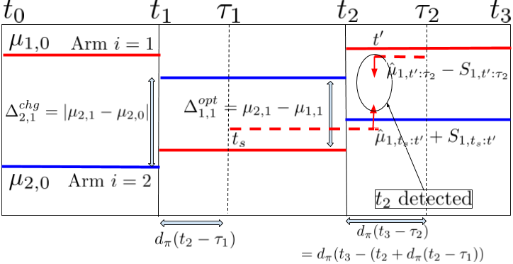
(a) A $2$-arm and $2$ changepoint scenario.

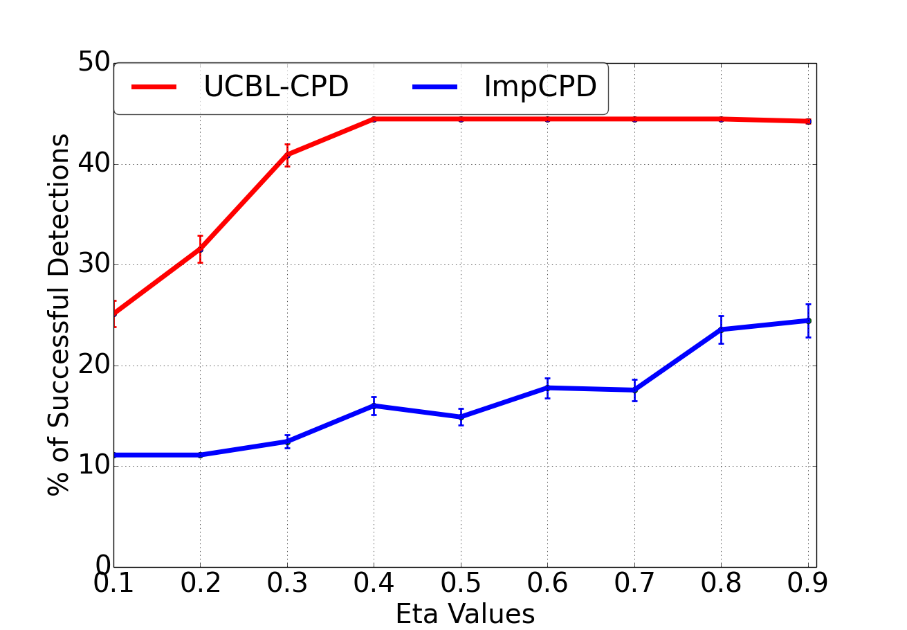
(b) Expt-$1$: The effect of $\eta$ on ImpCPD and UCBL-CPD

Figure 1: Illustration of Changepoint Detection

A reasonable detection policy $\pi$ has to contend with two things, 1) to find the optimal arm between $t_{g-1}$ to $t_{g}$ with high probability, 2) to detect abrupt changes and restart. Previous works (Liu et al., 2017), (Cao et al., 2018), (Besson and Kaufmann, 2019) have concentrated mainly on the assumption that at $t_{g}$ mean of any arm can change. Moreover, Cao et al. (2018), Besson and Kaufmann (2019) also consider the per-arm local changepoint setting forcing them to conduct additional exploration of arms to detect abrupt changes, leading to gap-independent results. We consider a slightly stricter global changepoint assumption 1 such that at every $t_{g},\forall g\in\mathcal{G}$ the mean of all the arm changes allowing us to derive stronger gap-dependent results. Additionally, the vast majority of the previous settings assumed that all changepoints are well-separated, and all changepoint gaps are significant so that they can be detected well in advance (see Table 1). Diverging from this line of thinking we propose a more realistic setting where there can be undetectable changepoint gaps and $\pi$ will not be able to detect all changepoints with high probability. This leads to assumption 2 such that for three consecutive changepoints $t_{g-1}$, $t_{g}$, and $t_{g+1}$, even if $t_{g}$ has low probability of detection due to large detection delay of $t_{g-1}$, sufficient number of observations are available to detect $t_{g+1}$. Finally, we introduce assumption 3 to restrict the scenario where a series of undetectable changepoint gaps for the same arms are encountered. An illustrative explanation of a $2$-arm $2$ changepoint scenario is shown in Table 1(a). Our main contributions are as follows:

1. Problem setup: We consider the more realistic setting where there can be undetectable changepoint gaps. In assumption 1 we assume that at each changepoint the mean of all the arms change which leads to the removal of forced exploration of arms allowing us to derive the first gap-dependent logarithmic regret for this setting. Additionally, assumption 2 and assumption 3 allows us to tackle some worst-case scenarios even when there are undetectable changepoint gaps.

2. Algorithmic: We propose two actively adaptive upper confidence bound (UCB) algorithms, referred to as UCBLaplace-Changepoint Detector (UCBL-CPD ) and Improved Changepoint Detector (ImpCPD ). Unlike CD-UCB (Liu et al., 2017), M-UCB (Cao et al., 2018) and CUSUM (Liu et al., 2017), UCBL-CPD and ImpCPD do not conduct forced exploration to detect changepoints. They divide the time into slices, and for each time slice, for every arm, they check the UCB, LCB mismatch based on past observations only to detect changepoints. While UCBL-CPD checks for every such combination of time slices, ImpCPD only checks at certain estimated points in time horizon and hence saves on computation time.

Table 1: Comparison of Algorithms

Algorithm	Type	T	G	Assumptions	Gap-Dependent	Gap-Independent
ImpCPD (ours)	Active	Y	N	1, 2, 3	Theorem 2	$\!O\left(\sqrt{GT}\right)$
UCBL-CPD (ours)	Active	N	N	1, 2, 3	Theorem 1	$\!O\left(\sqrt{GT}\log T\right)$
CUSUM	Active	Y	Y	1, 4, 5	N/A	$\!O\left(\sqrt{GT\log\frac{T}{G}}\right)$
M-UCB	Active	Y	Y	1${}^{\ref{footnote:0}}$, 4${}^{\text{\ref{footnote:1}}}$, 5${}^{\ref{footnote:2}}$	N/A	$\!O\left(\sqrt{GT\log T}\right)$
EXP3.R	Active	Y	N	5${}^{\text{\ref{footnote:2}}}$	N/A	$\!O\left(G\sqrt{T\log T}\right)$
DUCB	Passive	Y	Y	1${}^{\text{\ref{footnote:0}}}$, 5${}^{\text{\ref{footnote:2}}}$	N/A	$\!O\left(\sqrt{GT}\log T\right)$
SWUCB	Passive	Y	Y	1${}^{\text{\ref{footnote:0}}}$, 5${}^{\text{\ref{footnote:2}}}$	N/A	$\!O\left(\sqrt{GT\log T}\right)$
Lower Bound	Oracle	Y	Y	1, 3	Theorem 3	$\!\Omega\left(\sqrt{GT}\right)$

3. Regret bounds: The CDUCB, CUSUM uses the Hoeffding inequality and M-UCB uses McDiarmid’s inequality with union bound to obtain the regret bound. DUCB (Garivier and Moulines, 2011) and SWUCB (Garivier and Moulines, 2011) uses the peeling argument which results in slightly tighter concentration bound but both these techniques results in less tight bounds than the Laplace method of integration used for UCBL-CPD which has the strongest bound proposed for this setting. Moreover, UCBL-CPD has time-uniform bound as its confidence interval does not depend explicitly on $t$ as opposed to other methods. On the contrary, ImpCPD which is not anytime and has access to $T$ uses the usual union bound with geometrically increasing phase length to bound the regret. Both these proofs are of independent interest which can be used in other settings as well. A detailed comparison of the union, peeling and Laplace bound can be found in discussion 2. We prove the first gap-dependent logarithmic regret upper bound that consist of both the changepoint gaps ($\Delta^{chg}_{i,g}$) and optimality gaps ($\Delta^{opt}_{i,g}$) for each changepoint $g\!\in\!\mathcal{G}$, $i\!\in\!\mathcal{A}$ in Theorem 1, and 2 (under assumptions 1, 2, and 3). We introduce the hardness parameter $H_{1,g}$ and $H_{2,g}$ which captures the problem complexity of the piecewise i.i.d setting. For the gap-independent result we show in the challenging case when all the gaps are small such that for all $i\!\in\!\mathcal{A},g\!\in\!\mathcal{G}$, $\Delta^{opt}_{i,g}=\Delta^{chg}_{i,g}=\Delta(t_{g},\delta)$, $H_{1,g}\!=\!{K}{(\Delta(t_{g},\delta))^{-2}}$ and $H_{2,g}\!=\!1$, UCBL-CPD and ImpCPD achieves $\sqrt{GT}\log T$ and $\sqrt{GT}$ respectively (Table 1, and Corollary 1). We show that UCBL-CPD and ImpCPD perform very well across diverse piecewise i.i.d environments even when our modelling conditions do not hold (Section 5).

The rest of the paper is organized as follows. We first setup the problem in Section 2. Then in Section 3 we present the changepoint detection algorithms. Section 4 contains our main result, remarks and discussions. Section 5 contains numerical simulations, Section 6 contains related works, and we conclude in Section 7. The proofs are provided in Appendices in the supplementary material.

2 Problem Setup

2.1 Preliminaries

Let $t_{0}=1$ by convention, so that $t_{0}<\!t_{1}<\!\!\dots<\!\!t_{G}$. We introduce the time interval (piece) $\rho_{g}=[t_{g},t_{g+1}-1]$, so the piece $\rho_{g}$ starts at $t_{g}$ and ends at $t_{g+1}-1$. Let, $\mu_{i,g}$ be the expectation of an arm $i$ for the piece $\rho_{g}$. The learner does not know $t_{g},\forall g\in\mathcal{G}$ or even $|\mathcal{G}|$. The reward drawn for the $i$-th arm, when it is pulled, for the $t$-th time instant is denoted by $X_{i,t}$. We assume all rewards are bounded in $[0,1]$. $N_{i,\tau_{g}:\tau_{g+1}-1}$ denotes the number of times arm $i$ has been pulled between $\tau_{g}$ to $\tau_{g+1}-1$ timesteps for any sequence of increasing $(\tau_{g})_{g}$ of integers. Also, we define $\hat{\mu}_{i,\tau_{g}:\tau_{g+1}-1}$ as the empirical mean of the arm $i$ between $\tau_{g}$ to $\tau_{g+1}-1$ timesteps. We consider that on each arm i, the process generating the reward is piecewise mean constant according to the sequence $(t_{g})_{g}$. That is, if $\mu_{i,t}$ denotes the mean reward of arm i at time t, then $\mu_{i,t}$ has same value for all $t\in\rho_{g}$.

Definition 1.

We define $t_{g}$ as, $t_{g}=\min\{t>t_{g-1}:\exists i,\mu_{i,t-1}\neq\mu_{i,t}\}$.

Assumption 1.

(Global changepoint) We assume the global changepoint setting, that is $t_{g}=t$ implies $\mu_{i_{t-1}}\neq\mu_{i_{t}}$, for all $i\in\mathcal{A}$.

Definition 2.

The changepoint gap at $t_{g}$ for an arm $i\in\mathcal{A}$ between the segments $\rho_{g}$ and $\rho_{g+1}$ is denoted by $\Delta^{chg}_{i,g}=|\mu_{i,g}-\mu_{i,g+1}|.$

Thus, at each changepoint we assume that the mean of all the arm changes. Note, that this assumption is stricter than Liu et al. (2017), Cao et al. (2018), Besson and Kaufmann (2019) where at $t_{g}$, $\mu_{i_{t}}$ of any arm may or may not change requiring the forced exploration of all arms to detect changepoint. Next we incorporate a more general and realistic structure to our problem. We assume that at $t_{g}$ there could be undetectable changepoint gaps (Definition 4) and every changepoint $t_{g}$ need not be detectable with high probability but three consecutive changepoints $t_{g-1},t_{g}$ and $t_{g+1}$ must follow assumption 2. Now, we carefully setup our problem. First, we distinguish between any best detection policy $\pi^{*}$ which has observations exactly from $t_{g-1}$ and any reasonable detection policy $\pi$ which has observations after $t_{g-1}$ with some delay. We denote the delay of a policy $\pi$ restarting from $\tau_{g-1}\!>\!t_{g-1}$ as $d_{\pi}(t_{g}-\tau_{g-1})$. We define the minimum number of samples ${\color[rgb]{0,0,1}n(t_{g},\Delta,\delta)}$ required for an arm $i\in\mathcal{A}$ so that a deviation of $\Delta>0$ of $\hat{\mu}_{i,g-1}$ (or $\hat{\mu}_{i,g}$) from $\mu_{i,g-1}$ (or $\mu_{i,g}$) before (or after) the $t_{g}$-th changepoint can be controlled with $(1-\delta)$ probability. This is shown in Lemma 1. We then bound the delay of $\pi^{\ast}$ in detecting a changepoint at $t_{g}$ starting exactly from $t_{g-1}$ (Lemma 2). Finally, we define the detectable changepoint gap $\Delta(t_{g},\delta)$ based on the maximal delay of $\pi^{\ast}$ and $n(t_{g},\Delta,\delta)$.

Lemma 1.

(Control of large deviations) For our detection policy $\pi^{\ast}$ using estimated means starting exactly from $t_{g-1}$, it is sufficient to collect a minimum number of samples $n(t_{g},\Delta,\delta)=\lceil\frac{1}{2}\log(\frac{2(t-t_{g-1})^{2}}{\delta})/\Delta^{2}\rceil$ for a single arm $i\in\mathcal{A}$, a changepoint $g\in\mathcal{G}$ before or after $t_{g}$ so that $|\hat{\mu}_{i,g-1}-\mu_{i,g-1}|\leq\Delta$ or $|\hat{\mu}_{i,g}-\mu_{i,g}|\leq\Delta$ with $(1-\delta)$ probability and $t_{g-1}<t_{g}<t$.

Proof 1.

The proof of Lemma 1 is given in Appendix A.

Assumption 2.

(Separated Changepoints) We assume that for every two consecutive segments $\rho_{g-1}$ and $\rho_{g},\forall g\in\mathcal{G}$ all the three changepoints $t_{g-1},t_{g}$ and $t_{g+1}$ satisfy the following condition,

$$t_{g}\!+\!d_{\pi^{\ast}}\left(t_{g}\!-\!t_{g-1}\right)\!\leq\!t_{g}\!+\!\eta(t_{g+1}-t_{g})\!=\!\eta t_{g+1}+(1-\eta)t_{g}$$

where $\eta\in(0,1)$, $d_{\pi^{\ast}}(t_{g}-t_{g-1})$ is the maximal delay of best detection policy $\pi^{*}$ starting at $t_{g-1}$.

Using Lemma 1 and Assumption 2 now we properly define detectable changepoint gap $\Delta(t_{g},\delta)$ to be such $\Delta(t_{g},\delta)\geq\sqrt{\log(2(x^{2}/\delta))/2x}$ where $x=t_{g}+d_{\pi^{*}}(t_{g}-t_{g-1})-t_{g-1}$.

Lemma 2.

(Detection Delay) With the standard assumption that at $t_{g}$, $\Delta(t_{g},\delta)$ scales atleast as $\Omega(\sqrt{\frac{\log t}{t}})$ for $K$ arms, then to detect a deviation of $\Delta\geq\Delta(t_{g},\delta)$ at $t_{g}$ with $(1-\delta)$ probability, $\pi^{*}$ suffers a worst case maximum delay of $d_{\pi^{\ast}}(t_{g}\!-\!t_{g-1})\!\leq\!\!\left(\frac{C(t,\delta,\eta)K\log(\frac{t^{2}}{{\delta}})}{2(\Delta(t_{g},\delta))^{2}}\right)\!+\!K\delta$, where $C(t,\delta,\eta)\leq\eta\log(t/\delta)$.

Proof 2.

The proof of Lemma 2 is given in Appendix B.

Definition 3.

The $\Delta^{chg}_{i,g}$ for an arm $i\in\mathcal{A},g\in\mathcal{G}$ is a $\delta$-optimal changepoint gap if $\Delta^{chg}_{i,g}\geq\Delta(t_{g},\delta)$. Let $\mathcal{A}_{g}^{chg}$ denote only those arms $i\in\mathcal{A}$ whose $\Delta^{chg}_{i,g}\geq\Delta(t_{g},\delta)$ at the $t_{g}$-th changepoint.

Definition 4.

The $\Delta^{chg}_{i,g}$ for an arm $i\in\mathcal{A},g\in\mathcal{G}$ is an undetectable gap if $\sqrt{\frac{e}{T}}\!\!\leq\!\!\Delta^{chg}_{i,g}\!\!<\!\!\Delta(t_{g},\delta)$.

Definition 5.

A changepoint $t_{g}$ is undetectable changepoint if $\exists\Delta^{chg}_{i,g}$ at $t_{g}$ s.t. $\sqrt{\frac{e}{T}}\!\!\leq\!\!\Delta^{chg}_{i,g}\!\!<\!\!\Delta(t_{g},\delta)$.

Assumption 3.

(Isolated Changepoints) We assume that at $t_{g}$ each gap $\!\Delta^{chg}_{i,g}$ is either $\delta$-optimal or is undetectable. If $t_{g}$ is undetectable, then $\!\Delta^{chg}_{i,g-1}$ and $\!\Delta^{chg}_{i,g+1}$ for all $i\in\mathcal{A}$ are $\delta$-optimal gaps.

Discussion 1.

Thus, assumption 2 makes sure that $t_{g}+d_{\pi^{\ast}}(t_{g}-t_{g-1})$ stays away from $t_{g+1}$. This ensures that when restarting the detection strategy from $t_{g}+d_{\pi^{\ast}}(t_{g}-t_{g-1})$, the detection of $t_{g+1}$ will not be too much endangered. This is a mild assumption as without this, changepoints could be too frequent so that they cannot be detected on time before the next change happens. A $\delta$-optimal detectable changepoint gap requires a minimum sample of $n(t_{g},\Delta,\delta)$ to ensure that $\Delta$ deviation from the mean can be detected with $(1-\delta)$ probability (Lemma 1). An undetectable gap requires more than $n(t_{g},\Delta,\delta)$ samples or possibly unbounded samples for ensuring $\Delta\geq\Delta(t_{g},\delta)$ deviation. Assumption 3 ensures that there cannot be a series of undetectable gaps to avoid linear regret. If at $t_{g}$, $\Delta^{chg}_{i,g}$ is undetectable then $\Delta^{chg}_{i,g-1}$ and $\Delta^{chg}_{i,g+1}$ are $\delta$-optimal gaps. Policy $\pi$ has its maximal delay $d_{\pi}(t_{g}-\tau_{g-1})\geq d_{\pi^{\ast}}(t_{g}\!-\!t_{g-1})$ as it only has observation to detect $t_{g}$ from $\tau_{g-1}$ and not from $t_{g-1}$ (unlike $\pi^{*}$). $\pi$ tries to minimize $d_{\pi}(t_{g}\!-\!\tau_{g-1})$ in detecting $t_{g}$ such that $d_{\pi}(t_{g}\!-\!\tau_{g-1})\leq(1+\beta)d_{\pi^{\ast}}(t_{g}\!-\!t_{g-1})$ holds with high probability for some $\beta\in(0,1)$ and $\eta\in(0,1)$. This approach is different than the vast majority of current litertaure Cao et al. (2018), Liu et al. (2017), Besson and Kaufmann (2019) as they assume that all the previous changepoints can be detected with high probability or all changepoints have constant large separation between them which is unrealistic. In Lemma 2 the assumption that $\Delta(t_{g},\delta)$ scales atleast as $\Omega(\sqrt{\log t/t})$ is not a global minimum gap assumption as there could be smaller undetectable isolated gaps by assumption 3. In contrast Cao et al. (2018), Liu et al. (2017) assumes that all gaps are large enough to be detectable. For a large $d_{\pi}(t_{g}-\tau_{g-1})$, sufficient number of observations may not be available to detect $t_{g}$ but this will not endanger detection of $t_{g+1}$ by assumption 2 and 3. The effect of $\eta$ on our proposed algorithms is shown in Figure 1(b). The details of the environment are mentioned in section 5, experiment 1. The key takeaway is that lower $\eta$ values leads to lower subsequent segments $(t_{g+1}-t_{g})$. So detection policy $\pi^{*}$ starting exactly at $t_{g-1}$ has to have lower delay $d_{\pi^{\ast}}(t_{g}-t_{g-1})$ to successfully detect subsequent changepoints. Conversely, $\pi^{*}$ is deemed good if it has less delay for low $\eta$ values. UCBL-CPD has higher percentage of successful detection and less variance for all $\eta$ values than ImpCPD as it implements the Laplace bound as opposed to the loose union bound of ImpCPD .

Definition 6.

The optimality gap $\Delta^{opt}_{i,g}$ for an arm $i_{t^{\prime}}\neq i^{*}_{t^{\prime}},\forall t^{\prime}\in[t_{g-1},t_{g}-1]$ is $\Delta^{opt}_{i,g}=\mu_{i^{*},g}-\mu_{i,g}.$

2.2 Regret Definition

The objective of the learner is to minimize the cumulative regret till $T$, which is defined as, $R_{T}=\sum_{t^{\prime}=1}^{T}\mu_{i^{*}_{t^{\prime}}}-\sum_{t^{\prime}=1}^{T}\mu_{i_{t^{\prime}}}\mathbb{I}\{i_{t^{\prime}}\neq i^{*}_{t^{\prime}}\}$, where $T$ is the horizon, $\mu_{i^{*}_{t^{\prime}}}$ is the expected mean of the optimal arm at the $t^{\prime}$ timestep and $\mu_{i_{t^{\prime}}}\mathbb{I}\{i_{t^{\prime}}\neq i^{*}_{t^{\prime}}\}$ is the expected mean of the arm chosen by the learner at the $t^{\prime}$ timestep when it was not the optimal arm $i^{*}_{t^{\prime}}$. The expected regret of an algorithm after $T$ timesteps can be written as,

$$\mathbb{E}[R_{T}]=\mathbb{E}\!\left[\sum_{t^{\prime}=1}^{T}\mu_{i^{*}_{t^{\prime}}}-\sum_{t^{\prime}=1}^{T}\mu_{i_{t^{\prime}}}\mathbb{I}\{i_{t^{\prime}}\neq i^{*}_{t^{\prime}}\}\right] \overset{(a)}{=}\!\!\mathbb{E}\left[\sum_{g=1}^{G}\sum_{t^{\prime}=t_{g-1}}^{t_{g}}\!\mu_{i^{*}_{t^{\prime}}}\!-\!\sum_{g=1}^{G}\sum_{t^{\prime}=t_{g-1}}^{t_{g}}\!\mu_{i_{t^{\prime}}}\mathbb{I}\{i_{t^{\prime}}\neq i^{*}_{t^{\prime}}\}\!\right]$$

$$\overset{(b)}{=}\sum_{g=1}^{G}\sum_{i=1}^{K}\Delta^{opt}_{i,g}\mathbb{E}[N_{i,t_{g-1}:t_{g}}]$$

where $(a)$ is from Assumption 1, and $(b)$ from Definition 6.

2.3 Problem Complexity

We define the hardness of a changepoint $g\in\mathcal{G}$ using optimality and changepoint gaps by modifying the definitions of problem complexity as introduced in Audibert et al. (2010) for stochastic bandits. Let $\!{\color[rgb]{0,0,1}H_{1,g}}\!=\!\max\!\left\{\!\sum_{i=1}^{K}\!\frac{1}{(\Delta^{opt}_{i,g})^{2}},\sum_{i\in\mathcal{A}^{chg}_{g}}\!\frac{1}{(\Delta^{chg}_{i,g})^{2}}\!\right\}\text{, and }{\color[rgb]{0,0,1}H_{2,g}}\!=\!\!\frac{\Delta^{opt}_{\max,g+1}}{\Delta(t_{g},\delta)}$, where $\Delta^{opt}_{\max,g+1}=\max_{i\in\mathcal{A}}\Delta^{opt}_{i,g+1}$. The hardness parameter $H_{2,g}$ captures the tradeoff between the minimum detectable gap $\Delta(t_{g},\delta)$ and maximum optimality gap of the next changepoint $\Delta^{opt}_{\max,g+1}$ which serves as an upper bound to all such possible trade-offs at changepoint $g$. The relation between the above complexity terms can be derived as, $H_{2,g}\leq H_{1,g}\leq\frac{K}{(\Delta(t_{g},\delta))^{2}}(H_{2,g})$. Note that, $\frac{\Delta^{opt}_{i,g}}{\Delta^{chg}_{i,g}}\leq H_{2,g},\forall i\in\mathcal{A}^{chg}_{g},g\in\mathcal{G}$. In the challenging case when all gaps are small and equal i.e. $\Delta^{opt}_{i,g}=\Delta^{chg}_{i,g}=\Delta(t_{g},\delta),\forall i\in\mathcal{A},g\in\mathcal{G}$, then, $H_{1,g}={K}{(\Delta(t_{g},\delta))^{-2}},\text{ and }H_{2,g}=1$.

2.4 Repeating worst case

We think that both assumption 2 and 3 are required to avoid a combination of worst cases in absence of forced exploration. There can be a scenario where for each $g\in\mathcal{G}$, $\pi$ keeps on pulling sub-optimal arm $i$ and then $t_{g}$ happens. At $t_{g}$, $\Delta^{chg}_{i,g}$ is undetectable so $\pi$ does not restart. So at $t_{g+1}$, assumption 3 will prevent this. Furthermore, assumption 2 ensures that consecutive changepoints $t_{g-1}$, $t_{g}$ and $t_{g+1}$ are such that even if the detection of $t_{g}$ is a low probability event (undetectable changepoint), there are sufficient number of observations left to detect $t_{g+1}$.

3 Algorithms

We first introduce the policy UCBL-CPD in Algorithm 1 which is an adaptive algorithm based on the standard UCB1 (Auer et al., 2002a) approach. UCBL-CPD pulls an arm at every timestep as like UCB1 but has the time-uniform concentration bound that holds simultaneously for all timestep $t$. It calls upon the Changepoint Detection (CPD) subroutine in Algorithm 2 for detecting a changepoint. Note, that unlike CD-UCB, CUSUM, and M-UCB the UCBL-CPD does not conduct forced exploration to detect changepoints. UCBL-CPD is an anytime algorithm which does not require the horizon as an input parameter or to tune its parameter $\delta$. This is in stark contrast with CD-UCB, CUSUM, M-UCB, DUCB or SWUCB, that require the knowledge of $G$ or $T$ for optimal performance. we define the confidence interval of UCBL-CPD as follows:

$$S_{i,t_{s}:t_{p}} :=\sqrt{\left(1+\frac{1}{N_{i,t_{s}:t_{p}}}\right)\frac{\log(\sqrt{N_{i,t_{s}:t_{p}}+1}/\delta)}{2N_{i,t_{s}:t_{p}}}}\vspace*{-3em}$$ (1)

Algorithm 1 UCB Laplace CPD (UCBL-CPD )

1:Input: $\delta>0$;

2:Definition: $S_{i,t_{s}:tp}$ from (1)

3:Initialization: $t_{s}:=1$, $t_{p}:=1$.

4:Pull each arm once

5:for $t=K+1,..,T$ do

6:     Pull arm $j\in\mathop{\rm arg\,max}_{i\in\mathcal{A}}\left\{\hat{\mu}_{i,t_{s}:t_{p}}+S_{i,t_{s}:t_{p}}\right\}$, observe reward $X_{j,t}$.

7:     Update $\hat{\mu}_{j,t_{s}:t_{p}}$, $N_{j,t_{s}:t_{p}}:=N_{j,t_{s}:t_{p}}+1.$

8:     $t_{p}:=t_{p}+1.$

9:     if  (CPD($t_{s}$, $t_{p}$, $\delta$)) then

10:         Restart: Set $\hat{\mu}_{i,t_{s}:t_{p}}:=0$, $N_{i,t_{s}:t_{p}}:=0$, $\forall i\in\mathcal{A}$, $t_{s}:=t$, $t_{p}:=t_{s}$.

11:         Pull each arm once.      

Algorithm 2 Changepoint Detection($t_{s}$, $t_{p}$, $\delta$) (CPD)

1:for $i=1,..,K$ do

2:     for $t^{\prime}=t_{s},..,t_{p}$ do

3:         if $\big{(}\hat{\mu}_{i,t_{s}:t^{\prime}}+S_{i,t_{s}:t^{\prime}}<\hat{\mu}_{i,t^{\prime}+1:t_{p}}-S_{i,t^{\prime}+1:t_{p}}\big{)}$ or $\big{(}\hat{\mu}_{i,t_{s}:t^{\prime}}-S_{i,t_{s}:t^{\prime}}>\hat{\mu}_{i,t^{\prime}+1:t_{p}}+S_{i,t^{\prime}+1:t_{p}}\big{)}$ then

4:              Return True               

Next, we formally introduce the Improved Changepoint Detector (ImpCPD ) in Algorithm 3. This is a phase-based algorithm modeled on UCB-Improved (Auer and Ortner, 2010), which calls upon the Changepoint Detection Improved (CPDI) in Algorithm 4 for calculating scan statistics to actively detect changepoint. ImpCPD employs pseudo arm elimination like CCB (Liu and Tsuruoka, 2016) algorithm such that a sub-optimal arm $i$ is never actually eliminated but the active list $B_{m}$ is just modified to control the phase length. This helps ImpCPD adapt quickly because this is a global changepoint scenario and for some sub-optimal arm the changepoint maybe detected very fast. Another important divergence from UCB-Improved is the exploration parameter $0<\gamma\leq 1$ that controls how often the changepoint detection sub-routine CPDI is called. After every phase, $\epsilon_{m}$ is reduced by a factor of $\left(1+\gamma\right)$ instead of halving it (as like UCB-Improved) so that the number of pulls allocated for exploration to each arm is lesser than UCB-Improved. The CPDI sub-routine at the end of the $m$-th phase scans statistics so that if there is a significant difference between the sample mean of any two slices then it raises an alarm.

Algorithm 3 Improved Changepoint Detector (ImpCPD )

1:Input: Time horizon $T$, $0<\gamma\leq 1$.

2:Initialization: $B_{0}:=\mathcal{A}$, $m:=0$, $\epsilon_{0}:=1$, $\psi:=\frac{T^{2}}{K^{2}\log K}$, $\alpha:=\frac{3}{2}$.

$$M:=\left\lfloor\frac{1}{2}\log_{1+\gamma}\frac{T}{e}\right\rfloor,\hskip 5.69054pt\ell_{0}:=\left\lceil\frac{\log(\psi\epsilon_{0}^{2})}{2\epsilon_{0}}\right\rceil,L_{0}:=K\ell_{0}\text{, }t_{s}:=1\text{, }t_{p}:=1.$$

3:Definition: $S_{i,t_{s}:t_{p}}:=\sqrt{\dfrac{\alpha\log(\psi\epsilon_{m}^{2})}{2N_{i,t_{s}:t_{p}}}}$.

4:for $t=K+1,..,T$ do

5:     Pull arm $j\in\mathop{\rm arg\,max}_{i\in\mathcal{A}}\bigg{\{}\hat{\mu}_{i,t_{s}:t_{p}}+S_{i,t_{s}:t_{p}}\bigg{\}}$, observe reward $X_{j,t}$.

6:     $t:=t+1,t_{p}:=t_{p}+1$.

7:     if $t\geq L_{m}$ and $m\leq M$ then

8:         if CPDI($m,L_{m},\alpha,\psi$) then

9:              Restart: $B_{m}:=\mathcal{A}$; $m:=0$.

10:              Set $N_{i,t_{s}:t_{p}}:=0,\hat{\mu}_{i,t_{s}:t_{p}}:=0,\forall i\in\mathcal{A}$.

11:              $t_{s}:=t$, $t_{p}:=t_{s}$.

12:              Pull each arm once.

13:         else

14:              for $i\in\mathcal{A}$ do

15:                  if $\hat{\mu}_{i,t_{s}:t_{p}}+S_{i,t_{s}:t_{p}}<\max_{j\in\mathcal{A}}\{\hat{\mu}_{j,t_{s}:t_{p}}-S_{j,t_{s}:t_{p}}\}$ then

16:                       $|B_{m}|:=|B_{m}|-1$                                 

17:              Reset Parameters:

18:              $\epsilon_{m+1}:=\frac{\epsilon_{m}}{(1+\gamma)}$, $B_{m+1}:=B_{m}$.

19:              $\ell_{m+1}:=\left\lceil\dfrac{\log(\psi\epsilon_{m}^{2})}{2\epsilon_{m}}\right\rceil$.

20:              $L_{m+1}:=t+|B_{m+1}|\ell_{m+1}$.

21:              $m:=m+1.$      

Algorithm 4 Changepoint Detection Improved($m,L_{m},\alpha,\psi$) (CPDI)

1:Definition:$S_{i,t_{s}:L_{m}}=\sqrt{\dfrac{\alpha\log(\psi\epsilon_{m}^{2})}{2N_{i,t_{s}:L_{m}}}}$.

2:for $i=1,..,K$ do

3:     for $m^{\prime}=1,\ldots,m$ do

4:         if $\big{(}\hat{\mu}_{i,t_{s}:L_{m^{\prime}}}+S_{i,t_{s}:L_{m^{\prime}}}<\hat{\mu}_{i,L_{m^{\prime}}+1:L_{m}}-S_{i,L_{m^{\prime}+1}:L_{m}}\big{)}$ or $\big{(}\hat{\mu}_{i,t_{s}:L_{m^{\prime}}}-S_{i,t_{s}:L_{m^{\prime}}}>\hat{\mu}_{i,L_{m^{\prime}}+1:L_{m}}+S_{i,L_{m^{\prime}+1}:L_{m}}\big{)}$ then

5:              Return True               

Running time of algorithms: UCBL-CPD (like CD-UCB, CUSUM) calls the changepoint detection at every timestep, and ImpCPD calls upon the sub-routine only at end of phases. Hence, for a horizon $T$, $K$ arms, UCBL-CPD calls the changepoint detection subroutine $O(KT)$ times (memory requirements may scale as $O(KT^{2}/G)$) while ImpCPD calls the changepoint detection $O(K\!\log T)$ times, thereby substantially reducing the costly operation of calculating the changepoint detection statistics. By designing ImpCPD appropriately and modifying the confidence interval, this reduction comes at no additional cost in the order of regret (see Discussion 4 and Expt-5).

4 Main Results

We outline the main ideas to prove Theorem 1 and 2. In Lemma 3 we consider a single changepoint $g\in\mathcal{G}$ and a single arm $i\in\mathcal{A}^{chg}_{g}$ scenario where policy $\pi$ has observations from $t_{s}$ to $t$ for $t_{g-1}\leq t_{s}<t_{g}<t$ and $\Delta_{i,g}^{chg}$ is $\delta$-optimal. With the term $S_{i,t_{s}:t^{\prime}}$ as defined in equation (1), we define the bad event ${\color[rgb]{0,0,1}\xi^{chg}_{i,t}}=\!\big{\{}\!\exists t^{\prime}\!\!\in\![t_{s},t]\!:\big{(}\hat{\mu}_{i,t_{s}:t^{\prime}}\!-\!S_{i,t_{s}:t^{\prime}}\!>\!\hat{\mu}_{i,t^{\prime}\!+\!1:t}\!+\!S_{i,t^{\prime}\!+\!1:t}\big{)}\bigcup\big{(}\hat{\mu}_{i,t_{s}:t^{\prime}}\!+\!S_{i,t_{s}:t^{\prime}}\!<\!\hat{\mu}_{i,t^{\prime}\!+\!1:t}\!-\!S_{i,t^{\prime}\!+\!1:t}\big{)}\!\big{\}}$ which will lead to failure of detection of changepoint. Let $X_{i,t_{s}},X_{i,t_{s}+1},\ldots,X_{i,t^{\prime}}$ have their expectation as $\mu_{i,g-1}$ and $X_{i,t^{\prime}+1},X_{i,t^{\prime}+2},\ldots,X_{i,t}$ have their expectation as $\mu_{i,g}$. Then to tackle $|\mu_{i,g}-\mu_{i,g-1}|$, we study the concentration of $\hat{\mu}_{i,t_{s}:t^{\prime}}$ and $\hat{\mu}_{i,t^{\prime}+1:t}$ around $\mu_{i,g-1}$ and $\mu_{i,g}$ separately using Laplace method and combine them by using a simple union bound. These two quantities can also be jointly studied and yielding a robust concentration inequality as in (Maillard, 2019). We define the optimality bad event $\xi^{opt}_{i,g}$ as when the arm $i^{\ast}_{t^{\prime}}$ for $t^{\prime}\in[t_{g-1},t_{g}-1]$ have not been detected.

Lemma 3.

(Control of $\xi^{chg}_{i,t}$ by Laplace method) Let, $N_{i,t_{s}:t}$ be the number of times an arm $i$ is pulled from $t_{s}$ till the $t$-th timestep such that $t_{g-1}\leq t_{s}<t_{g}<t$, then at the $t$-th timestep for all $\delta\in(0,\frac{1}{4}]$ it holds that, $\mathbb{P}(\xi^{chg}_{i,t})\leq 4\delta$, where the event $\xi^{chg}_{i,t}$ is defined above.

Proof 2.

(Outline) We use the sub-Gaussian property of the bounded random variables to define a non-negative super-martingale $M_{t^{\prime}}^{\lambda}$. We show that it is well defined and introduce a new stopped version $M_{\tau}^{\lambda}$. By Fatou’s Lemma we show that it is bounded as well. Finally, we introduce an auxiliary variable $\Lambda$ independent of all other variables and use it to control $M_{\tau}^{\Lambda}$. We follow a similar procedure and define another non-negative super-martingale $M_{t-t^{\prime}}^{\lambda}$ and combine the result to bound the probability of the event $\xi^{chg}_{i,t}$. The proof is in Appendix C.

Discussion 2.

Time-uniform bound in (1) depends only on the number of pulls $N_{i,t_{s}:t_{p}}$ and implicitly on $t$ based on the parameter $\delta$. The concentration bounds based on peeling and union bound method depends explicitly on $t$ and has larger coefficients attached to them. In Table 2 we give a comparison over the three concentration bound method involving union bound, peeling and Laplace method and compare them empirically in experiment $5$. We provide the proof of the construction of concentration bound for our changepoint detection strategy by union bound in Lemma 4 in Appendix D for completeness. The $\log\log(t)$ scaling of the peeling method is not better than the one derived by the Laplace method, unless for huge timestep $t$ ($t>10^{6}$, for $\delta=0.05$ and any $\alpha>1$). Laplace method uses the sub-Gaussian nature of the variables to give such sharp concentration bounds as opposed to other methods.

Table 2: Comparison of Union, Peeling and Laplace method

Method	Confidence interval	Uniform over $t$
Union	$\sqrt{\frac{\log(4t^{2}/\delta)}{2N_{i,t_{s}:t^{\prime}}}}$	No
Peeling	$\sqrt{\frac{\alpha}{N_{i,t_{s}:t^{\prime}}}\log\left(\lceil\frac{\log(t)}{\alpha}\rceil\frac{1}{\delta}\right))}$, $\alpha>1$	No
Laplace	$\sqrt{\left(1+\frac{1}{N_{i,t_{s}:t^{\prime}}}\right)\frac{\log(\sqrt{N_{i,t_{s}:t^{\prime}}+1}/\delta)}{2N_{i,t_{s}:t^{\prime}}}}$	Yes

Theorem 1.

(Gap-dependent bound of UCBL-CPD ) For $\eta\geq\frac{6}{2\log t+1}$, $\delta=\frac{1}{t}$, the expected cumulative regret of UCBL-CPD using the CPD is given by,

$$\mathbb{E}_{\pi}[R_{t}]\!\! \leq\!\sum_{g=1}^{G}\!\bigg{\{}\!\!\underbrace{\sum_{i=1}^{K}\dfrac{6\log t}{\Delta^{opt}_{i,g}}}_{(a)}\!+\!\!\sum_{i\in\mathcal{A}_{g}^{chg}}\!\!\bigg{(}\!\!\underbrace{\dfrac{16H_{2,g}\log t}{\Delta^{chg}_{i,g}}}_{(b)}\!+\!\underbrace{\dfrac{30KH_{2,g}\log t}{\Delta(t_{g},\delta)}}_{(c)}\!\!\bigg{)}\!\!\bigg{\}}\!+\!\underbrace{\!\max_{i\in\mathcal{A}:\!\sqrt{\frac{e}{T}}\leq\!\Delta_{i}<\!\Delta(t_{g},\delta)}\Delta_{i}t\!}_{(d)}.$$

Proof 3.

(Outline) Let $\tau_{i,g}$ be the stopping time for $i$ and $\tau_{g}>t_{g}$ be the time $g$ is detected. We decompose the number of pulls $N_{i,1:t}$ into five parts (see eq (7), Appendix E). In part A we show that there exists a deterministic number of steps $\max\{N_{i,\min_{E}},N_{i,\min_{D}}\}$ before either UCBL-CPD discards sub-optimal arm $i$ or a false detection of changepoint happens between $\tau_{i,g-1}:t_{g}$. Part B handles the complementary event of part A by bounding the bad events $\xi^{opt}_{i,t}$ and $\xi^{chg}_{i,t}$ using Lemma 3 to control false detection of $t_{g}$. In part C we control the pulls accrued due to the worst case events that the changepoint has occurred and $i$ has not been sampled enough to detect changepoint ($N_{i,t_{g}:\tau_{i,g+1}}<N_{i,min_{D}}$) or is an undetectable gap ($\sqrt{\frac{e}{T}}\leq\Delta^{chg}_{i,g}<\Delta(t_{g},\delta)$). In this case, $\pi$ has to suffer the worst possible regret till a $\delta$-optimal changepoint is detected due to another arm (assumption 3) or a new non-isolated changepoint occurs (assumption 2). Part D controls the bad event that the changepoint is not detected from $t_{g}:\tau_{i,g}$ even when $N_{i,t_{g}:\tau_{i,g}}>N_{i,\min_{D}}$ using Lemma 3. Finally part E refers to the case when the changepoint $g$ is not detected from time $\tau_{g-1}$ till time $t$. We control it by showing that $d_{\pi}(t_{g}-\tau_{g-1})=d_{\pi}(t_{g}-(t_{g-1}+d_{\pi}(t_{g-1}-\tau_{g-2})))$ is bounded with high probability as long as $\eta>6/(2\log t+1)$ and assumption 2 holds for all $g\in\mathcal{G}$ (see step 6). We derive the value of $\eta$ from the base case. So, our approach is different than Cao et al. (2018), Liu et al. (2017), Besson and Kaufmann (2019) as part C, D and E requires careful handling of assumptions 2 and 3 which the previous works do not take. The proof of Theorem 1 is given in Appendix E. In Theorem 1, (a) is the regret suffered before finding the optimal arm between changepoints $g-1$ to $g$, (b) is the maximal regret for delayed detection of $g$, (c) is the regret suffered for total compounded delayed detection and $(d)$ for undetectable changepoints.

Theorem 2.

(Gap-dependent bound of ImpCPD ) For $\eta\geq\frac{8}{2\log T+1}$, $\delta=\frac{1}{T}$, the expected cumulative regret of ImpCPD using CPDI is upper bounded by,

$$\mathbb{E}_{\pi}[R_{T}]\leq\sum_{g=1}^{G}\sum_{i\in\mathcal{A}^{\prime}}\bigg{[}\underbrace{\frac{48KC_{1}\left(\gamma\right)\Delta^{opt}_{i,g}\log({T}/{K})}{(K\log K)^{-\frac{3}{2}}}}_{(a)}+\!\underbrace{\frac{16\log({T(\Delta^{opt}_{i,g})^{2}}/{K})}{(\Delta^{opt}_{i,g})}}_{(b)}\!\bigg{]}$$

$$\!+\!\sum_{g=1}^{G}\sum_{i\in\mathcal{A}^{chg}_{g}}\bigg{[}\!\underbrace{\frac{16H_{2,g}\log({T(\Delta^{chg}_{i,g})^{2}}/{K})}{(\Delta^{chg}_{i,g})}}_{(c)}+\!\underbrace{\frac{16KH_{2,g}\log({T(\Delta^{chg}_{i,g})^{2}}/{K})}{(\Delta(t_{g},\delta))}}_{(d)}\bigg{]}\!\!+\underbrace{\!\max_{i\in\mathcal{A}:\!\sqrt{\frac{e}{T}}\leq\!\Delta_{i}<\!\Delta(t_{g},\delta)}\Delta_{i}T\!}_{(e)}\vspace*{-1em}$$

where $\gamma\in(0,1]$ is exploration parameter, $C_{1}\left(\gamma\right)=\left(\frac{1+\gamma}{\gamma}\right)^{4}$, and $\mathcal{A}^{\prime}=\big{\{}i\in\mathcal{A}:\Delta^{opt}_{i,g}\geq\sqrt{\frac{e}{T}},\Delta^{chg}_{i,g}\geq\sqrt{\frac{e}{T}},\forall g\in\mathcal{G}\big{\}}$.

Proof 4.

(Outline) This proof closely follows the approach of Theorem 1. We carefully construct each geometrically increasing phase length $\ell_{m}$ so that the probability not pulling the optimal arm between two changepoints $g-1$ to $g$ is bounded. Simultaneously, we use the phase length $\ell_{m}$, confidence interval $S_{i,t_{s}:t_{p}}$ and exploration factor $\gamma$ and $\psi$ to control the bad event of not detecting the changepoint $g$. We use Chernoff-Hoeffding inequality to bound the probability of the bad events. We have to further balance $\ell_{m}$, and $S_{i,t_{s}:t_{p}}$ by carefully defining $\psi$ so that $\gamma$ is small enough and CPDI is called more often. We have to use additional union bounds to control the event that arms are getting pulled unequal number of times within each phase length. The proof is in Appendix F. In Theorem 2, (a) is the regret for calling the CPDI at end of phases, (b) is the regret for finding the optimal arm between changepoints $g-1$ and $g$, (c) is the regret for delayed detection of $g$, (d) is the regret suffered for total compounded delayed detection and $(e)$ for undetectable changepoints.

Discussion 3.

UCBL-CPD (Theorem 1) and ImpCPD (Theorem 2) performance is comparable to the best detection strategy (see Lemma 2) as they have the coefficient in their compounded detection delay of order $O(K)$ that is less than order $O(\eta\log(t/\delta))$ of $C(t,\delta,\eta)$ of $\pi^{\ast}$ when $\eta$ is greater than the respective values in the theorems. This is reasonable as in the bandit setup each arm $i\in\mathcal{A}$ might be pulled a logarithmic number of times before detecting a changepoint.

Corollary 1.

(Gap-independent bounds) In the challenging scenario, when all the gaps are equal and small, i.e. $\!\Delta^{opt}_{i,g}\!=\!\Delta^{chg}_{i,g}\!=\!\Delta(t_{g},\delta)=\!\!\sqrt{\frac{K\log(T/G)}{T/G}}\!>\!\Omega(\sqrt{\frac{\log t}{t}}),\forall i\!\!\in\!\!\mathcal{A},\forall g\!\!\in\mathcal{G}$, $t\!>\!\!\sqrt{T}$, $\delta\!=\frac{1}{T}$, $\gamma\!=0.05$, $\!G\geq\!\!{\log T}\!$ then worst case gap-independent regret bound of UCBL-CPD and ImpCPD is,

$$\mathbb{E}_{\text{{\color[rgb]{0.6,0,0}UCBL-CPD }}}[R_{T}]\leq O(\sqrt{GT}\log T),\text{ \hskip 20.00003pt }\mathbb{E}_{\text{{\color[rgb]{0.6,0,0}ImpCPD }}}[R_{T}] \leq C_{1}G^{1.5}K^{4.5}(\log K)^{2}+O(\sqrt{GT}).$$

Proof 5.

The proof of Corollary 1 follows from Theorem 1 and 2 and is given in Appendix G.

Discussion 4.

In Corollary 1, the largest contributing factor to the gap-independent regret of UCBL-CPD is of the order $O(\sqrt{GT}\log T)$, same as that of DUCB but weaker than CUSUM and SWUCB. The additional $O(\log T)$ factor is the cost UCBL-CPD must pay for not knowing $T$ and $G$. The largest contributing factor to the gap-independent regret of ImpCPD is of the order $O(\sqrt{GT})$. This is lower than the regret upper bound of DUCB, SWUCB, EXP3.R and CUSUM (Table 1). The smaller the value of the exploration parameter $\gamma$ the larger is the constant $C_{1}$ associated with the factor $GK^{4.5}(\log K)^{2}$. Now, $\gamma$ determines how frequently CPDI is called by ImpCPD and by modifying the confidence interval and phase-length we have been able to control the probability of not detecting the changepoint at the cost of additional regret that only scales with $K$ and not with $T$.

Theorem 3.

(Lower Bounds for $\pi^{o}$) The lower bound of an oracle policy $\pi^{o}$ for a horizon $T$, $K$ arms and $G$ changepoints is given by $\!\mathbb{E}_{\pi^{o}}[R_{T}]\geq\min\{\!\Omega(\sum\limits_{g=1}^{G}\sum\limits_{i=1}^{K}\!\frac{\log{(T/(GH_{1,g}))}}{(\Delta_{i,g}^{opt})}),\!\Omega(\sqrt{GT}\!)\}$.

Proof 7.

An oracle policy $\pi^{o}$ has access to the exact changpoints. The worst case scenario can occur when environment changes uniform randomly. A similar argument has also been made in the adaptive-bandit setting of (Maillard and Munos, 2011). So, let the horizon $T$ be divided into $G$ slices, each of length $(T/G)$. For each of these slices an oracle algorithm using OCUCB (Lattimore, 2015) should get the optimal SMAB regret without suffering any delay. The proof is in Appendix H.

Discussion 5.

This lower bound is weaker than the bound proposed in Wei et al. (2016) as they do not require the knowledge of $G$ or $T$. But we provide this for completion to discuss oracle-based bounds and also because the previous approaches do not touch upon this approach. For a non-oracle policy the additional trade-off between the changepoint gap and the next optimality gap is captured by $H_{2,g}$. As long as the delayed detection is bounded with high probability we should get a similar scaling for a good detection algorithm minimizing regret for each of these slices of length $(T/G)$. ImpCPD which has a gap-independent regret upper bound of $O(\sqrt{GT})$ reaches the lower bound of the policy $\pi^{o}$ in an order optimal sense. In the challenging case when all the gaps are same and small such that for all $i\in\mathcal{A},g\in\mathcal{G}$, $\Delta^{opt}_{i,g}=\Delta(t_{g},\delta)=\Delta^{chg}_{i,g}$, $H_{1,g}=K(\Delta(t_{g},\delta))^{-2}$ and $H_{2,g}=1$, then ImpCPD with a gap-dependent bound of $O\big{(}\sum\limits_{g=1}^{G}\sum\limits_{i=1}^{K}\frac{\log({T}/{H_{1,g}})}{\Delta_{i,g}^{opt}}\big{)}$ matches the gap dependent lower bound of $\pi^{o}$ except the factor $G$ in the log term (see Table 1).

5 Experiments

We compare UCBL-CPD and ImpCPD against Oracle Thompson Sampling (OTS), EXP3.R, Discounted Thompson Sampling (DTS), Discounted UCB (DUCB), Sliding Window UCB (SWUCB), Monitored-UCB (M-UCB) and CUSUM-UCB (CUSUM) in four environments . The oracle algorithm have access to the exact changepoints and are restarted at those changepoints.

5.1 Parameter Selection for Algorithms

For DTS we use the discount factor $\gamma=0.75$ as specified in (Raj and Kalyani, 2017) for slow varying environment. For DUCB we set $\gamma=1-\frac{1}{4}\sqrt{\frac{1}{T}}$ and for SWUCB we use the window size of $W=4\sqrt{T\log T}$ as suggested in Garivier and Moulines (2011). Note, that for implementing the two passive algorithms we do not use the knowledge of the number of changepoints $G$ to make these algorithms more robust, even though Garivier and Moulines (2011) suggests using $\gamma=1-\frac{1}{4}\sqrt{\frac{G}{T}}$ or $W=4\sqrt{\frac{T\log T}{G}}$ for optimal performance. For CUSUM, we need to tune four parameters, $M$ which is the minimum number of pulls required for each arm which must be first satisfied, parameter $\alpha$ which determines random uniform exploration between arms, and the CUSUM changepoint detection parameter $h$ and tolerance factor $\epsilon$. We choose $M=40$, $\alpha=\sqrt{\frac{G}{T}\log\left(\frac{T}{G}\right)}$, $\epsilon=0.1$ and $h=\log\left(\frac{T}{G}\right)$ (as suggested in Liu et al. (2017)) for both the experiments. Hence, CUSUM requires the knowledge of the number of changepoints in tuning its parameters. Similarly, Exp3.R requires tuning of three parameters $\delta$, $\gamma$ and $H$ for changepoint detection. We choose $\delta=\sqrt{\frac{\log T}{KT}}$, $\gamma=\sqrt{\frac{K\log K\log T}{T}}$ and $H=\sqrt{T\log T}$ as suggested in Allesiardo et al. (2017). Finally, for UCBL-CPD we choose $\delta=\frac{1}{t}$ (Theorem 1) and for and ImpCPD we choose $\delta=\frac{1}{T}$, $\gamma=0.05$ (Corollary 1).

5.2 Numerical Simulations

Experiment 1 (Bernoulli $3$ arms): This experiment is conducted to test the performance of algorithms in Bernoulli distribution over a short horizon $T=4000$ and and small number of arms $K=3$. There are $3$ changepoints in this testbed and the expected mean of the arms changes as shown in equation (2) ($\eta<0.5$). From the Figure 2(a) we can clearly see that UCBL-CPD and ImpCPD detect the changepoints at $t=1000$ and $t=2000$ with a small delay and restarts. However, because of the small changepoint gap at $t=3000$ it takes some time to adapt and restart. UCBL-CPD and ImpCPD perform better than all the passively adaptive algorithms like DTS, DUCB, SWUCB, and actively adaptive algorithm like EXP3.R, CUSUM and is only outperformed by OUCB1 and OTS which have access to the oracle. The performance of UCBL-CPD is similar to ImpCPD in this small testbed. Because of the short horizon and a small number of arms, the adaptive algorithms CUSUM and EXP3.R are outperformed by passive algorithms DUCB, SWUCB, and DTS.

$$r_{1}=0.1,r_{2}=0.2,r_{3}=0.9\textbf{, if }t=[1,1000];$$

$$r_{1}=0.4,r_{2}=0.9,r_{3}=0.1\textbf{, if }t=[1001,2000];$$

$$r_{1}=0.5,r_{2}=0.1,r_{3}=0.2\textbf{, if }t=[2001,3000];$$

$$r_{1}=0.2,r_{2}=0.2,r_{3}=0.3\textbf{, if }t=[3001,4000].$$ (2)

Experiment 2 (Jester dataset): This experiment is conducted to test the performance of algorithms when our model assumptions are violated. We evaluate on the Jester dataset (Goldberg et al., 2001) which consist of over 4.1 million continuous ratings of 100 jokes from 73,421 users collected over 5 years. We use Jester because there exist a high number of users who have rated all the jokes, and so we do not have to use any matrix completion algorithms to fill the rating matrix. The goal of the learner is to suggest the best joke when a new user comes to the system. We consider $20$ users who have rated all the $100$ jokes and use SVD to get a low rank approximation of this rating matrix. Most of the users belong to three classes who prefer either joke number $49$, $88$, or $90$. We uniform randomly sample $2$ users from each of the $3$ classes ($49$, $88$, $90$). Then we divide the horizon $T=200000$ into $6$ changepoints starting from $t=1$ and at an interval of $25000$ we introduce a new user from one of the three classes in round-robin fashion starting from users who prefer joke $49$. We change the user at changepoints to simulate the change of distributions of arms and hence a single learning algorithm has to adapt multiple times to learn the best joke for each user. A real-life motivation of doing this may stem from the fact that running an independent bandit algorithm for each user is a costly affair and when users are coming uniform randomly a single algorithm may learn quicker across users if all the users prefer a few common items. Note, that we violate assumption 2 and 3 because the horizon is small, the number of arms is large and gaps are too small to be detectable with sufficient delay. In Figure 2(b) we see that ImpCPD and UCBL-CPD outperforms all other actively adaptive algorithms. ImpCPD and UCBL-CPD is only able to detect $2$ of the $6$ changepoints and restart while CUSUM failed to detect any of the changepoints. Note that UCBL-CPD and ImpCPD performs slightly worse than SWUCB, DUCB in this testbed. This shows that when gaps are small, and changepoints are less separated, all the change-point detection techniques will perform badly in those regimes.

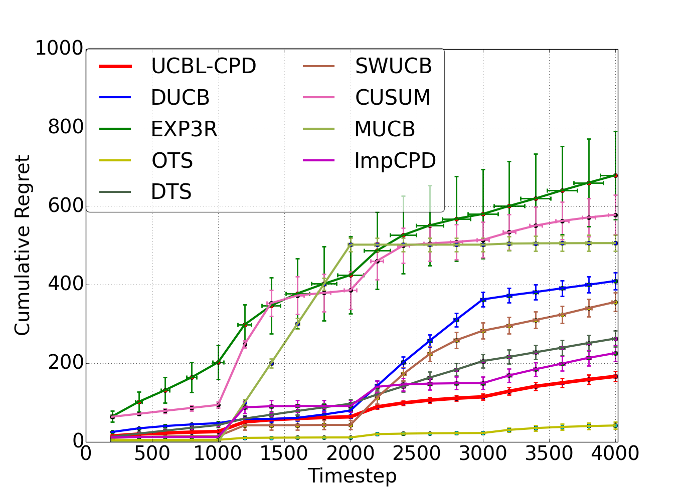
(a) Expt-$1$: $3$ Bernoulli-distributed arms.

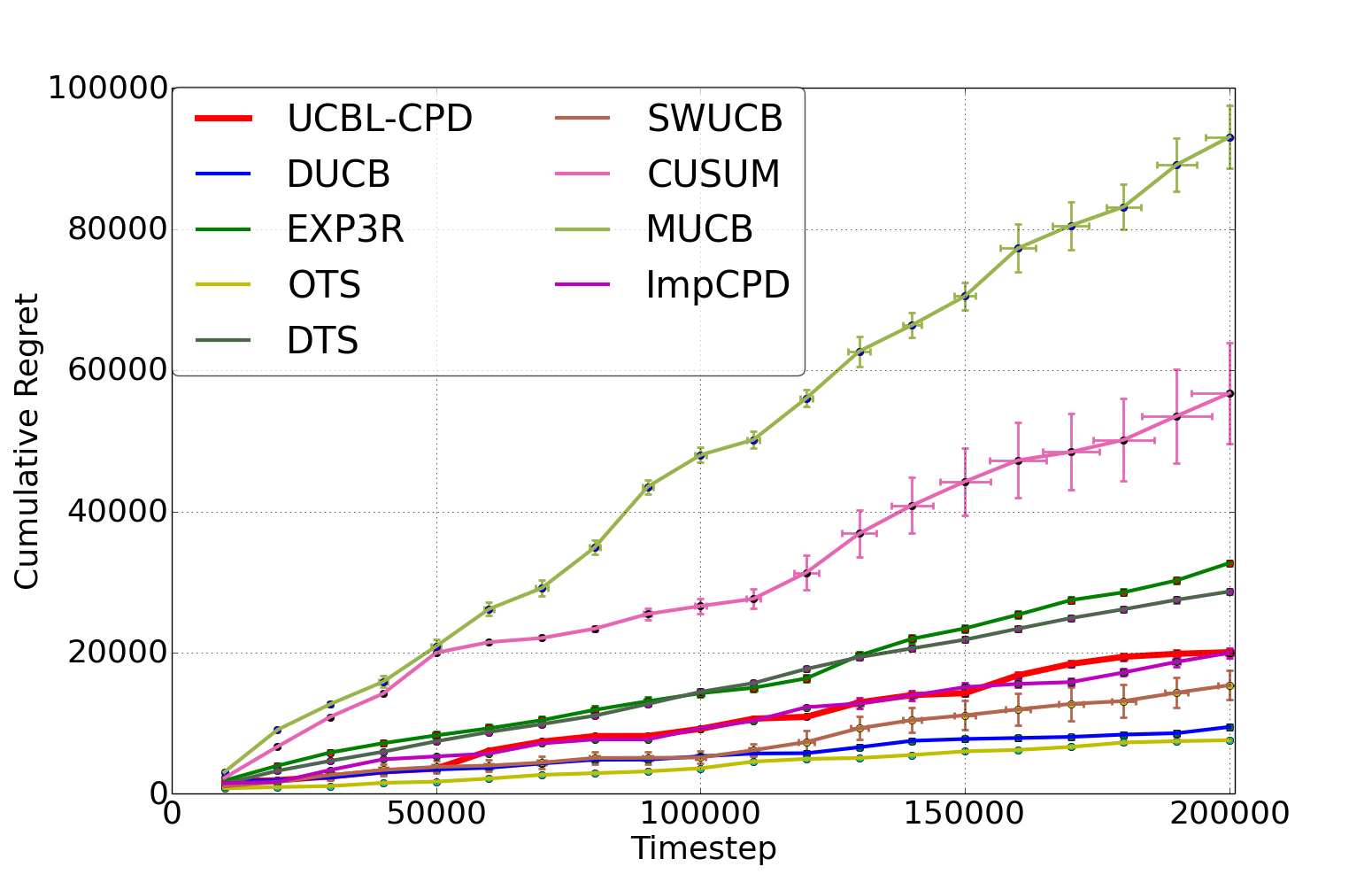
(b) Expt-$2$: $20$ Users, $100$ items, Rank $3$ approximation of Jester Dataset

Figure 2: Cumulative regret for various bandit algorithms on two piecewise i.i.d environments

Experiment 3 (Gaussian $10$ arms): This experiment is conducted to test the performance of algorithms in Gaussian distribution where the distribution flips between two alternating environments. This experiment involves $10$ arms with Gaussian distribution. There are $3$ changepoints in this testbed where the horizon is $T=15000$ and the expected mean of the arms changes as shown in equation 3. The variance of all arms $i\in\mathcal{A}$ is set as $\sigma_{i}^{2}=0.25$ so that the sub-Gaussian distributions remain bounded in $[0,1]$ with high probability. The experiment is shown in Figure 3(a) where we can clearly see that UCB-CPD and ImpCPD detect all the changepoints at $t=1875$, $t=5001$ and $t=9001$ with a small delay and restarts. ImpCPD clearly performs better than all the passively adaptive algorithms like DUCB and DTS, actively adaptive algorithm like EXP3.R and is only outperformed by OTS which have access to the oracle.

$$r_{1:4}=0.4-0.1^{1:4},r_{5}=0.45,r_{6}=0.55,r_{7:10}=0.6+0.1^{5-1:4}\textbf{ if }t=[1,1875];$$

$$r_{4:1}=0.6+0.1^{5-4:1},r_{5}=0.55,r_{6}=0.45,r_{7:10}=0.4-0.1^{4:1}\textbf{ if }t=[1876,5000];$$

$$r_{1:4}=0.4-0.1^{1:4},r_{5}=0.45,r_{6}=0.55,r_{7:10}=0.6+0.1^{5-1:4}\textbf{ if }t=[5001,9000];$$

$$r_{4:1}=0.6+0.1^{5-4:1},r_{5}=0.55,r_{6}=0.45,r_{7:10}=0.4-0.1^{4:1}\textbf{ if }t=[9001,15000].$$ (3)

Experiment 4 (Comparison of $4$ approaches): In figure 3(b) we compare UCB-CPD, ImpCPD , UCBL-CPD and UCBP-CPD for experiment 1 with $3$ Bernoulli Distributed arms. Note, that UCB-CPD and ImpCPD uses Chernoff-Hoeffding inequality to derive their confidence interval, with ImpCPD additionally having the knowledge of the time horizon $T$. UCBP-CPD ($\alpha=1.5$) uses peeling argument which uses the confidence interval mentioned in Table 2 and UCBL-CPD uses the confodence interval derived by Laplace method. In figure 3(b) we see that the changepoint detection method using the Laplace method performs very well and outperforms the algorithms using confidence interval obtained union and peeling method.

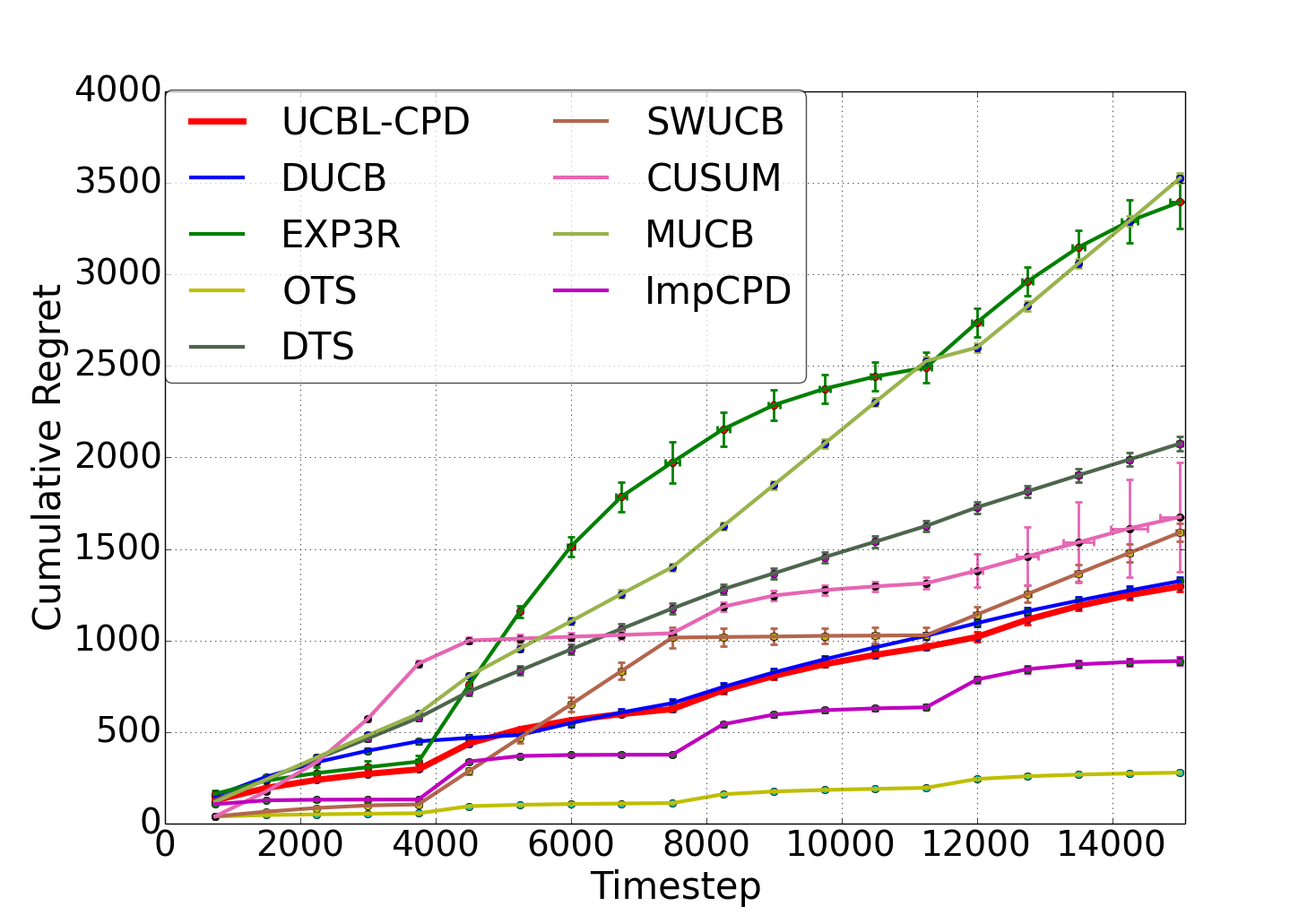
(a) Expt-$3$: $10$ Gaussian-distributed arms.

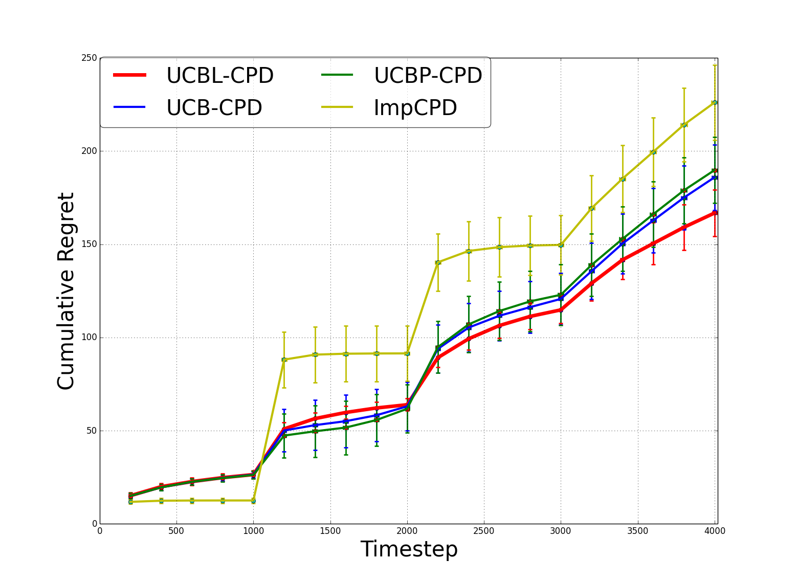
(b) Expt-$4$: $3$ Bernoulli-distributed arms.

Figure 3: Additional Experiments 1.

Experiment 5 (Comparison of running time): In figure 4(a) we compare the running time of ImpCPD and UCBL-CPD for the experiment 3 with $10$ Gaussian Distributed arms (see equation 3). We test on different horizon length starting from $T=5000$ till $T=14000$ and average over $50$ times the performance of each algorithm on each of those horizon lengths. We run this experiment on a single core of 2.8 GHz Intel Core i7 processor. From the figure 4(a) we can clearly see that ImpCPD which has a runtime of $O(K\log T)$ clearly outperforms UCBL-CPD which has a runtime of $O(KT)$ as discussed in Section 3.

Experiment 6 (Movielens Dataset): In this experiment we use another real life dataset to test the performance of our algorithm over unequal time intervals between changepoints. We experiment with the Movielens dataset from February 2003 (Harper and Konstan, 2016), where there are 6k users who give 1M ratings to 4k movies. Again we obtain a rank-2 approximation of the dataset over 20 users and 100 movies. The users either prefer movie $91$ (group 1) or $99$ (group 2). Now we divide the horizon $T=6000$ into two changepoints at $t=1000$ and $t=3000$. For the time interval $t\in[1,1000]$ we choose one user from group 1, then for $t\in[1001,3000]$ we choose another user from group 2 and finally for the last piece $t\in[3001,6000]$ we choose a different user from group 1 again. Since we wanted to test only over a short horizon with unequal time intervals between changepoints, we choose only the top $10$ preferred movies (arms) over all users. We use the rating of each user to the movies (arms) as the mean of a Bernoulli Distribution. From Figure 4 (or Figure LABEL:fig:61) we see that in this $10$ arm short horizon Bernoulli testbed UCBL-CPD and CUSUM perform really well and their performance matches the performance of the oracle algorithms OTS.

(a) Expt-$5$: Running Time of UCBL-CPD and ImpCPD for $10$ Gaussian-distributed arms.

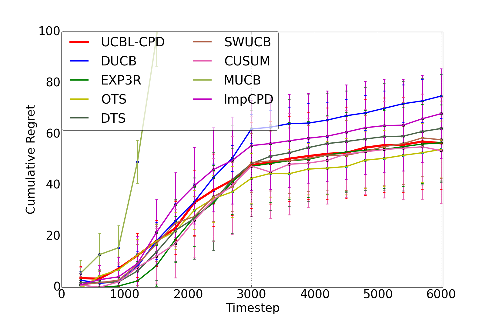
(b) Expt-$6$: Cumulative regret of different algorithms in Movielens dataset

Figure 4: Additional Experiments 2.

6 Related Works

The piecewise i.i.d setting is more general than the stochastic MAB (SMAB) setting and the adversarial setting. In the SMAB setting, the distribution associated with each arm is fixed throughout the time horizon whereas in the adversarial setting the distribution for each arm can change at any time step $t$. So for SMAB, $G=1$ whereas in the adversarial setting $G=T$. In the piecewise setting $G$ usually scales as $o(\sqrt{T})$ (Besson and Kaufmann, 2019). The upper confidence bound (UCB) algorithms, which are a type of index-based frequentist strategy, were first proposed in Agrawal (1995) and the first finite-time analysis for the stochastic setting for this class of algorithms was proved in Auer et al. (2002a). Strong minimax results for the SMAB setting was obtained in Audibert and Bubeck (2009), Auer and Ortner (2010), Lattimore (2015). For a detailed survey of SMAB refer to Bubeck and Cesa-Bianchi (2012), Lattimore and Szepesvári (2018). Following assumption 1, we can give minimax (see 2.4.3 in Bubeck and Cesa-Bianchi (2012)) regret bounds that incorporates the Hardness factor $H_{1,g}$ (introduced in Audibert et al. (2010), best-arm identification) which characterizes how difficult is the environment and depends on both $\Delta^{chg}_{i,g}$ and $\Delta^{opt}_{i,g}$. Also, for this setting we need an additional hardness parameter $H_{2,g}$ which captures the trade-off between optimality and changepoint gaps. We conjecture that an order optimal regret upper bound in the piecewise i.i.d setting of the order

$$\min\left\{O\left(\sum_{g=1}^{G}\sum_{i=1}^{K}\frac{H_{2,g}\log(T/(GH_{1,g}))}{\Delta^{opt}_{i,g}}\right),O\left(\sqrt{GT}\right)\right\}$$

is attainable. Obtaining such optimal minimax bound for SMAB was discussed in Audibert and Bubeck (2009), Auer and Ortner (2010), Bubeck and Cesa-Bianchi (2012) and solved in Lattimore (2016). We further extend the results to piecewise i.i.d algorithms (for a specific setting) which is non-trivial given the changepoint and optimality gaps have to be tackled independently.

Next, we survey some of the works for the piecewise i.i.d setting. Previous algorithms for this setting can be broadly divided into passive and actively adaptive algorithms. Passive algorithms like Discounted UCB (DUCB) (Kocsis and Szepesvári, 2006), Sliding Window UCB (SWUCB) (Garivier and Moulines, 2011) and Discounted Thompson Sampling (DTS) (Raj and Kalyani, 2017) do not actively try to detect changepoints and thus perform badly when changepoints are of large magnitude and are well-separated. The actively adaptive algorithm EXP3.R (Allesiardo et al., 2017) is an adaptive alternative to EXP3.S (Auer et al., 2002b) which was proposed for arbitrary changing environments. But EXP3.R is primarily intended for adversarial environments and thus is conservative when applied to a piecewise i.i.d. environment. The recently introduced actively adaptive algorithms CD-UCB (Liu et al., 2017), CUSUM (Liu et al., 2017) and M-UCB (Cao et al., 2018) rely on additional forced exploration for changepoint detection. With $\alpha$ probability they employ some changepoint detection mechanism or pull the arm with highest UCB with $(1-\alpha)$ probability (exploitation). This $\alpha$ depends on either knowledge of minimum gap, $G$ or $T$. CUSUM (Liu et al., 2017) performs a two-sided CUSUM test to detect changepoints and it empirically outperforms CD-UCB. CUSUM and M-UCB requires the knowledge of $G$ and $T$ for tuning $\alpha$ and CUSUM theoretical guarantees only hold for Bernoulli rewards for widely separated changepoints.

In Garivier and Moulines (2011) the authors showed that the regret upper bound of DUCB and SWUCB are respectively $O(\sqrt{GT}\log T)$ and $O(\sqrt{GT\log T})$, where $G$ is the total number of changepoints and $T$ is the time horizon which are known apriori. Furthermore, Garivier and Moulines (2011) showed that the cumulative regret in this setting is lower bounded in the order of $\Omega(\sqrt{T})$.The Restarting EXP3 (REXP3) (Besbes et al., 2014) behave pessimistically as like EXP3.S but restart after pre-determined phases. Hence, REXP3 can also be termed as a passively adaptive algorithm. The actively adaptive strategies like Adapt-EVE (Hartland et al., 2007), Windowed-Mean Shift (Yu and Mannor, 2009), EXP3.R (Allesiardo et al., 2017), CUSUM (Liu et al., 2017) try to detect the changepoints and restart. The regret bound of Adapt-EVE is still an open problem, whereas the regret upper bound of EXP3.R is $O(G\sqrt{T\log T})$ and that of CUSUM is $O(\sqrt{GT\log(T/G)})$. Note, that the regret bound of CUSUM is only valid for Bernoulli distributions. CUSUM wrongly applies Hoeffding inequality to a random number of pulls (see eq (31), (32) in Liu et al. (2017)) which raises serious concerns about the validity of the rest of their analysis. Also, there are Bayesian strategies like the Memory Bandits by (Alami et al., 2016) and Global Change-Point Thompson Sampling (GCTS) (Mellor and Shapiro, 2013) which uses Bayesian changepoint detection to locate the changepoints. However, the regret bound of Memory Bandits and GCTS is an open problem and has not been proved yet. Both of these algorithms require very high memory usage and so have been excluded from the experiments.

Another approach involves the Generalized Likelihood Ratio Test which was studied by Maillard (2019) and Besson and Kaufmann (2019). This is a different approach than others and looks at the ratio of the likelihood of the sequence of rewards coming from two different distributions and calculates the sufficient statistics to detect changepoints.

7 Conclusions and Future Works

We studied the piecewise i.i.d environment under assumption 1, 2 and 3 such that actively adaptive algorithms do not need to conduct forced exploration to detect changepoints even when there are undetectable changepoint gaps. We studied two UCB algorithms, UCBL-CPD and ImpCPD which are adaptive and restarts once the changepoints are detected. We derived the first gap-dependent logarithmic bounds for the piecewise i.i.d. setting incorporating the hardness factor. The anytime UCBL-CPD uses the Laplace method to derive sharp concentration bound, and ImpCPD achieves the order optimal regret bound which is an improvement over all the existing algorithms (in a specific challenging setting). Empirically, they perform very well in various environments and is only outperformed by oracle algorithms. Future works include incorporating the knowledge of localization in these adaptive algorithms and carefully investigate the dependence on $K$ in the bounds.

Acknowledgments

This work has been supported by CPER Nord-Pas de Calais/FEDER DATA Advanced data science and technologies 2015-2020, the French Ministry of Higher Education and Research, Inria Lille – Nord Europe, CRIStAL, and the French Agence Nationale de la Recherche (ANR), under grant ANR-16-CE40-0002 (project BADASS).

A Proof of Minimum Samples (Lemma 1)

Proof 1.

We consider a single arm $i\in\mathcal{A}$, single changepoint scenario such that $g=1$ (ignoring the expositions). Let, $t>t_{g}>t_{g-1}$. For the arm $i\in\mathcal{A}$, let $X_{i,t_{g-1}},X_{i,t_{g-1}+1},X_{i,t_{g-1}+2},\ldots,X_{i,t_{g}-1}$ be i.i.d real valued random variables having mean $\mu_{i,g-1}$ and $X_{i,t_{g}},X_{i,t_{g}+1},X_{i,t_{g}+2},\ldots,X_{i,t}$ be i.i.d real valued random variables having mean $\mu_{i,g}$. Let all random variables be bounded in $[0,1]$. We want to show that for the arm $i$, after $n(t_{g},\Delta,\delta)=\left\lceil\dfrac{\log(\frac{2(t-t_{g-1})^{2}}{\delta})}{2\Delta^{2}}\right\rceil$ samples have been collected for it before (or after) $t_{g}$, the probability of large deviation of empirical mean $\hat{\mu}_{i,g}$ (or $\hat{\mu}_{i,g-1}$) from $\mu_{i,g}$ (or ${\mu}_{i,g-1}$) is bounded.

Step 1. (Deviation Event): Let $\xi_{i,t}$ be the event that $\hat{\mu}_{i,g-1}$ or $\hat{\mu}_{i,g}$ is deviating from $\mu_{i,g-1}$ or $\mu_{i,g}$ by more than $\Delta$ at timestep $t>t_{g}$. Let $\Delta$ be the minimum gap the learner needs to detect a change for the $i$-th arm after the $g$-th changepoint has occurred. Note, that $t_{g-1},t_{g},n(t_{g},\Delta,\delta)$ and $t$ are not random variables.

$$\xi_{i,t} =\bigg{\{}\exists t_{g-1}<t_{g}-1,\Delta>0:\left|\dfrac{1}{t_{g}-n(t_{g},\Delta,\delta)-1}\sum_{s=n(t_{g},\Delta,\delta)}^{t_{g}-1}X_{i,s}-\mu_{i,g-1}\right|>\Delta\bigg{\}}$$

$$\bigcup\bigg{\{}\exists t>t_{g},\Delta>0:\left|\dfrac{1}{t-n(t_{g},\Delta,\delta)}\sum_{s=n(t_{g},\Delta,\delta)}^{t}X_{i,s}-\mu_{i,g}\right|>\Delta\bigg{\}}.$$

Step 2. (Bounding the probability of deviation event): Now we bound the probability of the detection event by using Chernoff-Hoeffding bound.

$$\mathbb{P}(\xi_{i,t}) =\underbrace{\mathbb{P}\bigg{(}\exists t_{g-1}<t_{g}-1,\Delta>0:\left|\dfrac{1}{t_{g}-n(t_{g},\Delta,\delta)-1}\sum_{s=n(t_{g},\Delta,\delta)}^{t_{g}-1}X_{i,s}-\mu_{i,g-1}\right|>\Delta\bigg{)}}_{\textbf{term A}}$$

$$+\underbrace{\mathbb{P}\bigg{(}\exists t_{g}<t,\Delta>0:\left|\dfrac{1}{t-n(t_{g},\Delta,\delta)}\sum_{s=n(t_{g},\Delta,\delta)}^{t}X_{i,s}-\mu_{i,g}\right|>\Delta\bigg{)}}_{\textbf{term B}}.$$

First, we bound the probability of the term (A),

$$\mathbb{P}(A) =\mathbb{P}\bigg{(}\left|\dfrac{1}{t_{g}-n(t_{g},\Delta,\delta)-1}\sum_{s=n({t_{g}},\Delta,\delta)}^{t_{g}-1}X_{i,s}-\mu_{i,g-1}\right|>\Delta\bigg{)}\leq\sum_{n=n(t_{g},\Delta,\delta)}^{t_{g}-1}\sum_{s=n(t_{g},\Delta,\delta)}^{n}2\exp\left(-2\left(\Delta\right)^{2}s\right)$$

$$\overset{(a)}{\leq}\sum_{n=t_{g-1}}^{t_{g}-1}\sum_{s=t_{g-1}}^{n}2\exp\left(-2\left(\Delta\right)^{2}\dfrac{\frac{1}{2}\log(\frac{2(t-t_{g-1})^{2}}{\delta})}{\left(\Delta\right)^{2}}\right)$$

$$\leq\sum_{n=t_{g-1}}^{t_{g}-1}\sum_{s=t_{g-1}}^{n}\dfrac{\delta}{2(t-t_{g-1})^{2}}\leq\frac{\delta}{2}$$

where, in $(a)$ we substitute $s\geq n(t_{g},\Delta,\delta)$. Similarly, we can show that for $s\geq n(t_{g},\Delta,\delta)=\left\lceil\dfrac{\log(\frac{2(t-t_{g-1})^{2}}{\delta})}{2\Delta^{2}}\right\rceil$ for term (B),

$$\mathbb{P}(B)=\mathbb{P}\bigg{(}\exists t_{g}<t,\Delta>0:\left|\dfrac{1}{t-n(t_{g},\Delta,\delta)}\sum_{s=n(t_{g},\Delta,\delta)}^{t}X_{i,s}-\mu_{i,g}\right|>\Delta\bigg{)}\leq\frac{\delta}{2}.$$

Summing over all of the above cases and taking a union bound, we can show that, $\mathbb{P}(\xi_{i,t})\leq\delta$.

B Proof of Detection Delay of $\pi^{*}$ (Lemma 2)

Proof 2.

From Lemma 1 we know that a minimum sample of $n(t_{g},\Delta,\delta)$ is sufficient for an arm $i\in\mathcal{A}$ to control $\Delta$ deviation from $\mu_{i,g-1}$ or $\mu_{i,g}$ on both sides of $t_{g}$ with $(1-\delta)$ probability. Let $\Delta\geq\Delta(t_{g},\delta)$. The changepoint detection policy may pull each arm $i=1,\ldots,K$, at most $n(t_{g},\Delta,\delta)-1$ times before finally detecting the changepoint for the $K$-th arm. Let, $t_{g}<\tau_{g}=t<t_{g+1}$ be the time the best policy $\pi^{\ast}$ detects the changepoint $g$ starting exactly from $t_{g-1}$.

Step 1 (Deviation event): Following Lemma 1 we define the deviation event $\xi_{i,t}$ for an arm $i\in\mathcal{A}$ and $t>t_{g}$ as

$$\xi_{i,t} =\bigg{\{}\exists t_{g-1}<t_{g}-1,\Delta\geq\Delta(t_{g},\delta):\left|\dfrac{1}{t_{g}-n(t_{g},\Delta,\delta)-1}\sum_{s=n(t_{g},\Delta,\delta)}^{t_{g}-1}X_{i,s}-\mu_{i,g-1}\right|>\Delta\bigg{\}}$$

$$\bigcup\bigg{\{}\exists t>t_{g},\Delta\geq\Delta(t_{g},\delta):\left|\dfrac{1}{t-n(t_{g},\Delta,\delta)}\sum_{s=n(t_{g},\Delta,\delta)}^{t}X_{i,s}-\mu_{i,g}\right|>\Delta\bigg{\}}.$$

such that after sampling the arm $i$ for $n(t_{g},\Delta,\delta)$ times the deviation of $\hat{\mu}_{i,g-1}$ (or $\hat{\mu}_{i,g}$) from $\mu_{i,g-1}$ (or $\mu_{i,g}$) is bounded with probability $(1-\delta)$.

Step 2 (Total Delay): The delay $d_{\pi^{\ast}}(t_{g}-t_{g-1})$ for detection policy $\pi^{*}$ can be upper bounded as,

$$d_{\pi^{\ast}}(t_{g}-t_{g-1}) =\sum_{i=1}^{K}\bigg{[}N_{i,t_{g-1}:t_{g}}+\mathbb{P}(\xi_{i,g})\bigg{]}$$

$$\leq(K-1)(n(t_{g},\Delta,\delta)-1)+n(t_{g},\Delta,\delta)+K\delta$$

$$\leq C(t_{g},\delta,\eta)K\dfrac{\log(\frac{2(t-t_{g-1})^{2}}{\delta})}{2\Delta(t_{g},\delta)^{2}}+K\delta$$

where, $C(t,\delta,\eta)$ depends on $t,\delta$ and $\eta$. Now, given that $t_{g-1},t_{g}$ and $t_{g+1}$ follow Assumption 2 such that $t_{g}+d_{\pi^{\ast}}(t_{g}-t_{g-1})\leq t_{g}+\eta(t_{g+1}-t_{g})$ holds. Then,

$$C(t,\delta,\eta)K\dfrac{\log(\frac{2(t-t_{g-1})^{2}}{\delta})}{2\Delta(t_{g},\delta)^{2}}+K\delta\leq\eta(t_{g+1}-t_{g})$$

$$\Leftrightarrow C(t,\delta,\eta)\leq\eta\dfrac{(t_{g+1}-t_{g})\Delta(t_{g},\delta)^{2}}{2K\log(t/\delta)}-K\delta\Delta(t_{g},\delta)^{2}.$$

Now, with a standard assumption that at $t_{g}$, $\Delta\geq\Delta(t_{g},\delta)$ scales atleast as $\Omega(\sqrt{\frac{\log t}{t}})$ for all $i\in\mathcal{A}$, $t_{g+1}-t_{g}\leq t$ and $\delta\in(0,1)$ we get,

$$C(t,\delta,\eta)\leq\dfrac{\eta(t_{g+1}-t_{g})\log(t)/t}{2K\log(t/\delta)}<\eta\log(t/\delta).$$

C Proof of Control of bad-event by Laplace method (Lemma 3)

Proof 3.

We start by noting that for any arm $i\in\mathcal{A}_{g}^{chg}$, $\pi$ detects a change-point if,

$$\hat{\mu}_{i,t_{s}:t^{\prime}}-S_{i,t_{s}:t^{\prime}}>\hat{\mu}_{i,t^{\prime}+1:t}+S_{i,t^{\prime}+1:t},\text{ or } \hat{\mu}_{i,t_{s}:t^{\prime}}+S_{i,t_{s}:t^{\prime}}<\hat{\mu}_{i,t^{\prime}+1:t}-S_{i,t^{\prime}+1:t}.$$ (4)

where for any $t^{\prime}\in[t_{s},t]$ we define confidence interval term $S_{i,t_{s}:t^{\prime}}$ for an arm $i\in\mathcal{A}$ at the $t$-th timestep as $S_{i,t_{s}:t^{\prime}}=\sqrt{\dfrac{(N_{i,t_{s}:t^{\prime}}+1)\log(\frac{\sqrt{(N_{i,t_{s}:t^{\prime}}+1)}}{\delta})}{2N_{i,t_{s}:t^{\prime}}^{2}}}$.

Step 1.(Define Bad Event:) Let, $(X_{i,t})_{t\geq t_{s}}$ be a sequence of non-negative independent random variables defined on a probability space $(\omega,\mathcal{F},\mathbb{P})$, is bounded in $[0,1]$. Let $X_{i,t_{s}},X_{i,t_{s}+1},\ldots,X_{i,t^{\prime}}$ have their expectation as $\mu_{i,g-1}$ and $X_{i,t^{\prime}+1},X_{i,t^{\prime}+2},\ldots,X_{i,t}$ have their expectation as $\mu_{i,g}$. Let $\mathcal{F}_{i,t}$ be an increasing sequence of $\sigma$-fields of $\mathcal{F}_{i}$ such that for each $t$, $\sigma(X_{i,t_{s}},\ldots,X_{i,t})\subset\mathcal{F}_{i,t}$ and for $q>t$, $X_{i,q}$ is independent of $\mathcal{F}_{i,t}$. We define a bad event $\xi^{chg}_{i,t}$ for an arm $i\in\mathcal{A}^{chg}_{g}$ as the complementary of events in (4) such that,

$$\xi^{chg}_{i,t} = \bigg{\{}\exists t^{\prime}\in[t_{s},t]:\big{(}\hat{\mu}_{i,t_{s}:t^{\prime}}-S_{i,t_{s}:t^{\prime}}\leq\hat{\mu}_{i,t^{\prime}+1:t}+S_{i,t^{\prime}+1:t}\big{)}$$ (5)

$$\bigcup\big{(}\hat{\mu}_{i,t_{s}:t^{\prime}}+S_{i,t_{s}:t^{\prime}}\geq\hat{\mu}_{i,t^{\prime}+1:t}-S_{i,t^{\prime}+1:t}\big{)}\bigg{\}}.$$

Step 2.(Define stopping times): We define a stopping time $\tau_{i,g}$ and $\tau^{\prime}_{i,g}$ for a $t^{\prime}\in[t_{s},t]$ such that,

$$\tau_{i,g}=\min\left\{\exists t^{\prime}:\big{(}\hat{\mu}_{i,t_{s}:t^{\prime}}-S_{i,t_{s}:t^{\prime}}\leq\hat{\mu}_{i,t^{\prime}+1:t}+S_{i,t^{\prime}+1:t}\big{)}\right\},$$

$$\tau^{\prime}_{i,g}=\min\left\{\exists t^{\prime}:\big{(}\hat{\mu}_{i,t_{s}:t^{\prime}}+S_{i,t_{s}:t^{\prime}}\geq\hat{\mu}_{i,t^{\prime}+1:t}-S_{i,t^{\prime}+1:t}\big{)}\right\}.$$

Step 3.(Define a super-martingale): We define the quantity $M_{t^{\prime}}^{\lambda}$, for any $t^{\prime}\in\mathbb{N}$ and for any $\lambda\in\mathbb{R}$ such that,

$$M_{t^{\prime}}^{\lambda}=\exp\left(\sum_{s=t_{s}}^{t^{\prime}}\left(\lambda(X_{i,s}-\mu_{i,t_{s}:t^{\prime}})-\dfrac{\lambda^{2}}{8}\right)\right).$$

Since $X_{i,t_{s}},X_{i,t_{s}+1},\ldots,X_{i,t^{\prime}}$ are i.i.d random variables bounded in $[0,1]$ we can consider them as $\frac{1}{2}$-sub-Gaussian; we can show that the quantity $M_{t^{\prime}}^{\lambda},\forall t^{\prime}\in\mathbb{N}$ is a non-negative super-martingale because, 1) $M_{t^{\prime}}^{\lambda}$ is $\mathcal{F}_{i,t^{\prime}-1}$ measurable, 2) $\mathbb{E}[|M_{t^{\prime}}^{\lambda}|]<\infty,\forall t\in\mathbb{N}$, and 3) $\mathbb{E}[M_{t^{\prime}+1}^{\lambda}|\mathcal{F}_{i,t^{\prime}}]\leq M_{t^{\prime}}^{\lambda},\forall t^{\prime}\in\mathbb{N}$.

So, $M_{t^{\prime}}^{\lambda}$ is well defined. Also, we can show that $\mathbb{E}[|M_{t^{\prime}}^{\lambda}|]\leq 1,\forall t^{\prime}\in\mathbb{N}$ and so $\log(\mathbb{E}[M_{t^{\prime}}^{\lambda}])\leq 0$ is also satisfied. By convergence theorem we can show that $M_{\infty}^{\lambda}=\lim_{t^{\prime}\rightarrow\infty}M_{t^{\prime}}^{\lambda}$ is also well defined. Now, we introduce a new stopped version of $M_{t^{\prime}}^{\lambda}$ such that $Q_{t^{\prime}}^{\lambda}=M^{\lambda}_{\min\{\tau_{i,g},t\}}$. By Fatou’s Lemma we can show that,

$$\mathbb{E}[M_{\tau_{i,g}}^{\lambda}]=\mathbb{E}[\lim\inf_{t^{\prime}\rightarrow\infty}Q_{t^{\prime}}^{\lambda}]\leq\lim\inf_{t^{\prime}\rightarrow\infty}\mathbb{E}[Q_{t^{\prime}}^{\lambda}]\leq 1.$$

Hence,$M_{\tau_{i,g}}^{\lambda}$ is well defined and $\mathbb{E}[M_{\tau_{i,g}}^{\lambda}]\leq 1$.

Step 4.(Introduce auxiliary variable): In this step we introduce an auxiliary variable $\Lambda=\mathcal{N}(0,4)$ which is independent of all other variables. The standard deviation of $\Lambda$ is $2$ since we are considering only $\frac{1}{2}$-sub-gaussian random variables. Hence, $\mathbb{E}[M_{\tau_{i,g}}^{\lambda}]=\mathbb{E}[\mathbb{E}[M_{\tau_{i,g}}^{\Lambda}|\Lambda]]\leq 1$. Let, $S_{t^{\prime}}=t^{\prime}\left(\frac{\sum_{s=t_{s}}^{t^{\prime}}X_{i,s}}{t^{\prime}}-\mu_{i,g-1}\right)$, then we can show that,

$$M_{t^{\prime}}=\dfrac{1}{\sqrt{8\pi}}\int_{\mathbb{R}}\exp\left(\lambda S_{t^{\prime}}-\dfrac{\lambda^{2}t^{\prime}}{8}-\dfrac{\lambda^{2}}{8}\right)d\lambda =\dfrac{1}{\sqrt{8\pi}}\int_{\mathbb{R}}\exp\left(-\left(\lambda\sqrt{\dfrac{t^{\prime}+1}{8}}-\dfrac{\sqrt{2}S_{t^{\prime}}}{\sqrt{t^{\prime}+1}}\right)^{2}+\dfrac{2S_{t^{\prime}}^{2}}{t^{\prime}+1}\right)d\lambda$$

$$\leq\exp\left(\dfrac{2S_{t^{\prime}}^{2}}{t^{\prime}+1}\right)\dfrac{1}{\sqrt{8\pi}}\int_{\mathbb{R}}\exp\left(-\lambda^{2}\dfrac{t^{\prime}+1}{8}\right)d\lambda$$

$$=\exp\left(\dfrac{2S_{t^{\prime}}^{2}}{t^{\prime}+1}\right)\dfrac{\sqrt{8\pi}}{\sqrt{8\pi(q+1)}}$$

$$\log(\sqrt{t^{\prime}+1}M_{t^{\prime}}) =\dfrac{2S_{t^{\prime}}^{2}}{t^{\prime}+1}$$

$$S_{t^{\prime}} =\sqrt{\dfrac{t^{\prime}+1}{2}\log(\sqrt{t^{\prime}+1}M_{t^{\prime}})}$$

From this we determine the confidence interval as $S_{i,t_{s}:t^{\prime}}=\sqrt{\dfrac{(N_{i,t_{s}:t^{\prime}}+1)\log(\frac{\sqrt{N_{i,t_{s}:t^{\prime}}+1}}{\delta})}{2N_{i,t_{s}:t^{\prime}}^{2}}}$.

Step 5.(Minimum pulls before $\tau_{i,g}$ and $\tau^{\prime}_{i,g}$): We define $N_{i,\min_{D}}$ as the minimum number of pulls before $\tau_{i,g}$ such that the event $|\mu_{i,g}-\mu_{i,g-1}|>2S_{i,t_{s}:\tau_{i,g}}$ is true with high probability. Then, for $N_{i,t_{s}:\tau_{i,g}}\geq N_{i,\min_{D}}=\dfrac{4\log(t\sqrt{t})}{(\Delta^{chg}_{i,g})^{2}}$ we can show that,

$$S_{i,t_{s}:\tau_{i,g}} =\sqrt{\dfrac{(N_{i,t_{s}:\tau_{i,g}}+1)\log(\frac{\sqrt{N_{i,t_{s}:\tau_{i,g}}+1}}{\delta})}{2N_{i,t_{s}:\tau_{i,g}}^{2}}}\leq\sqrt{\left(1+\dfrac{1}{t}\right)\dfrac{\log(\frac{\sqrt{(t+1)}}{\delta})}{2N_{i,t_{s}:\tau_{i,g}}}}$$

$$\leq\sqrt{\left(1+\dfrac{1}{t}\right)\dfrac{(\Delta^{chg}_{i,g})^{2}\log(\frac{\sqrt{(t+1)}}{\delta})}{8\log(t\sqrt{t})}}\leq\dfrac{\Delta^{chg}_{i,g}}{2}.$$

Similar result also holds for $\tau^{\prime}_{i,g}$ such that a minimum number of pulls $N_{i,\min_{D}}$ is required for $|\mu_{i,g}-\mu_{i,g-1}|>2S_{i,t_{s}:\tau^{\prime}_{i,g}}$ to be true with high probability.

Step 6.(Bound the probability of bad event): To bound the probability of bad event $\xi^{chg}_{i,t}$ it suffices to show that,

$$\mathbb{P} \left(N_{i,t_{s}:\tau_{i,g}}(\hat{\mu}_{i,t_{s}:\tau_{i,g}}-\mu_{i,g-1})\leq\sqrt{\dfrac{N_{i,t_{s}:\tau_{i,g}}+1}{2}\log\left(\dfrac{\sqrt{N_{i,t_{s}:\tau_{i,g}}+1}}{\delta}\right)}\right)$$

$$\leq\mathbb{P}\left(M_{\tau_{i,g}}\geq\dfrac{1}{\delta}\right)\overset{(a)}{\leq}\dfrac{\mathbb{E}[M_{\tau_{i,g}}]}{\frac{1}{\delta}}\overset{(b)}{\leq}\delta$$

where, in $(a)$ we use Markov inequality and $(b)$ comes from step 3. Similarly, we can define another super-martingale $M_{t-t^{\prime}}$ and follow the above procedure to show that

$$\mathbb{P}\left(N_{i,t^{\prime}+1:\tau_{i,g}}(\hat{\mu}_{i,t^{\prime}+1:\tau_{i,g}}-\mu_{i,g})\geq\sqrt{\dfrac{N_{i,t^{\prime}+1:\tau_{i,g}}+1}{2}\log\left(\dfrac{\sqrt{N_{i,t^{\prime}+1:\tau_{i,g}}+1}}{\delta}\right)}\right)\leq\delta$$

Hence, the probability that the change-point for the arm $i$ is not detected by first condition of $\xi^{chg}_{i,t}$ for any $\tau_{i,g}\in[t_{s},t]$ is bounded by $2\delta$. Again, for the second condition we can proceed in a similar way and show that for all $t^{\prime}\in[t_{s},t]$,

$$\mathbb{P}\bigg{(}\hat{\mu}_{i,g-1}+S_{i,t_{s}:\tau_{i,g}}\geq\hat{\mu}_{i,\tau^{\prime}_{i,g}+1:t}-S_{i,\tau^{\prime}_{i,g}+1:t}\bigg{)}\leq 2\delta.$$

Hence, we can bound the probability of the bad event $\xi^{chg}_{i,t}$ for an arm $i\in\mathcal{A}^{chg}_{g}$ for any $\tau_{i,g},\tau^{\prime}_{i,g}\in[t_{s},t]$ by taking the union of all the events above and get, $\mathbb{P}\{\xi^{chg}_{i,t}\}\leq 4\delta$.

D Proof of Control of bad-event by Union Bound method

The UCB-CPD algorithm is exactly like Algorithm 1 but uses the definition of $S_{i,t_{s}:t_{p}}$ as $\sqrt{\frac{\log(\frac{4t^{2}}{\delta})}{2N_{i,t_{s}:t_{p}}}}$.

Lemma 4.

(Control of bad-event by Union Bound method) Let, $\mu_{i,g}$ be the expected mean of an arm $i$ for the piece $\rho_{g}$, $N_{i,t_{s}:t}$ be the number of times an arm $i$ is pulled from $t_{s}$ till the $t$-th timestep such that $t>t_{g}$, then at the $t$-th timestep for all $\delta\in(0,1]$ it holds that,

$$\mathbb{P}\bigg{(}\!\exists t^{\prime}\!\!\in\![t_{s},t]\!:\big{(}\hat{\mu}_{i,t_{s}:t^{\prime}}\!-\!S_{i,t_{s}:t^{\prime}}\!>\!\hat{\mu}_{i,t^{\prime}\!+\!1:t}\!+\!S_{i,t^{\prime}\!+\!1:t}\big{)}\bigcup\big{(}\hat{\mu}_{i,t_{s}:t^{\prime}}\!+\!S_{i,t_{s}:t^{\prime}}\!<\!\hat{\mu}_{i,t^{\prime}\!+\!1:t}\!-\!S_{i,t^{\prime}\!+\!1:t}\big{)}\!\bigg{)}\leq\delta$$

where $S_{i,t_{s}:t^{\prime}}=\sqrt{\dfrac{\log(\frac{4t^{2}}{\delta})}{2N_{i,t_{s}:t^{\prime}}}}$.

Proof 4.

We define confidence interval term $S_{i,t_{s}:t^{\prime}}$ for an arm $i\in\mathcal{A}^{chg}_{g}$ at the $t$-th timestep as $S_{i,t_{s}:t^{\prime}}=\sqrt{\dfrac{\log(\frac{4t^{2}}{\delta})}{2N_{i,t_{s}:t^{\prime}}}}$ and $t_{s}$ is an arbitrary restarting timestep.

Step 1.(Define Bad Event): We define a bad event $\xi^{chg}_{i,t}$ for the arm $i$ as the complementary of events in Eq (4) such that,

$$\xi^{chg}_{i,t} = \bigg{\{}\exists t^{\prime}\in[t_{s},t]:\big{(}\hat{\mu}_{i,t_{s}:t^{\prime}}-S_{i,t_{s}:t^{\prime}}\leq\hat{\mu}_{i,t^{\prime}+1:t}+S_{i,t^{\prime}+1:t}\big{)}$$ (6)

$$\bigcup\big{(}\hat{\mu}_{i,t_{s}:t^{\prime}}+S_{i,t_{s}:t^{\prime}}\geq\hat{\mu}_{i,t^{\prime}+1:t}-S_{i,t^{\prime}+1:t}\big{)}\bigg{\}}.$$

Step 2.(Define stopping times): We define a stopping time $\tau_{i,g}$ and $\tau^{\prime}_{i,g}$ for a $t^{\prime}\in[t_{s},t]$ such that,

$$\tau_{i,g}=\min\left\{\exists t^{\prime}:\big{(}\hat{\mu}_{i,t_{s}:t^{\prime}}-S_{i,t_{s}:t^{\prime}}\leq\hat{\mu}_{i,t^{\prime}+1:t}+S_{i,t^{\prime}+1:t}\big{)}\right\},$$

$$\tau^{\prime}_{i,g}=\min\left\{\exists t^{\prime}:\big{(}\hat{\mu}_{i,t_{s}:t^{\prime}}+S_{i,t_{s}:t^{\prime}}\geq\hat{\mu}_{i,t^{\prime}+1:t}-S_{i,t^{\prime}+1:t}\big{)}\right\}.$$

Step 3.(Minimum pulls before $\tau_{i,g}$ and $\tau^{\prime}_{i,g}$): We define $N_{i,\min_{D}}$ as the minimum number of pulls before $\tau_{i,g}$ such that the event $|\mu_{i,g}-\mu_{i,g-1}|>2S_{i,t_{s}:\tau_{i,g}}$ is true with high probability. Then, for $N_{i,t_{s}:\tau_{i,g}}\geq N_{i,\min_{D}}=\dfrac{2\log(\frac{4t^{2}}{\delta})}{(\Delta^{chg}_{i,g})^{2}}$ we can show that,

$$S_{i,t_{s}:\tau_{i,g}}=\sqrt{\dfrac{\log(\frac{4t^{2}}{\delta})}{2N_{i,t_{s}:\tau_{i,g}}}}\leq\sqrt{\dfrac{\log(\frac{4t^{2}}{\delta})}{2N_{i,\min_{D}}}}\leq\sqrt{\dfrac{(\Delta^{chg}_{i,g})^{2}\log(\frac{4t^{2}}{\delta})}{4\log(\frac{4t^{2}}{\delta})}}\leq\dfrac{\Delta^{chg}_{i,g}}{2}.$$

Similar result also holds for $\tau^{\prime}_{i,g}$ such that a minimum number of pulls $N_{i,\min_{D}}$ is required for $|\mu_{i,g}-\mu_{i,g-1}|>2S_{i,t_{s}:\tau^{\prime}_{i,g}}$ to be true with high probability.

Step 4.(Bounding the probability of bad event): In this step we bound the probability of the bad event $\xi^{chg}_{i,t}$ in Eq (6).

Let $X_{i,t_{s}},X_{i,t_{s}+1},\ldots,X_{i,t^{\prime}}$ have their expectation as $\mu_{i,g-1}$ and $X_{i,t^{\prime}+1},X_{i,t^{\prime}+2},\ldots,X_{i,t}$ have their expectation as $\mu_{i,g}$. Then we define the event $\xi_{1}=\{\exists q\in[N_{i,\min_{D}},t^{\prime}]:\hat{\mu}_{i,q:t^{\prime}}\leq\mu_{i,g-1}-S_{i,q:t}\}$. Starting with the first condition of $\xi^{chg}_{i,t}$ and applying the Chernoff-Hoeffding inequality we can show that for a $\tau_{i,g}\in[t_{s},t]$,

$$\mathbb{P}(\xi_{1})\leq\sum_{t^{\prime}=N_{i,\min_{D}}}^{t}\sum_{q=N_{i,\min_{D}}}^{t^{\prime}}\mathbb{P}\bigg{(}\dfrac{\sum_{s=1}^{q}X_{i,s}}{q}\leq\mu_{i,g-1}-\dfrac{\log(\frac{4t^{2}}{\delta})}{2q}\bigg{)} \leq\!\!\!\!\sum_{t^{\prime}=N_{i,\min_{D}}}^{t}\sum_{q=N_{i,\min_{D}}}^{t^{\prime}}\exp\left(-2.\dfrac{\log(\frac{4t^{2}}{\delta})}{2q}q\right)$$

$$\leq\sum_{t^{\prime}=1}^{t}\sum_{q=1}^{t^{\prime}}\dfrac{\delta}{4t^{2}}\leq\frac{\delta}{4}.$$

Again, defining the event $\xi_{2}=\{\exists q\in[N_{i,\min_{D}},t^{\prime}]:\hat{\mu}_{i,q:t^{\prime}}\geq\mu_{i,g}+S_{i,q:t^{\prime}}\}$ and proceeding similarly as above, we can show that for a $\tau^{\prime}_{i,g}\in[t_{s},t]$,

$$\mathbb{P}(\xi_{2})\leq\sum_{t^{\prime}=N_{i,\min_{D}}}^{t}\sum_{q=N_{i,\min_{D}}}^{t^{\prime}}\mathbb{P}\bigg{(}\dfrac{\sum_{s=1}^{q}X_{i,s}}{q}\geq\mu_{i,g}+\dfrac{\log(\frac{4t^{2}}{\delta})}{2q}\bigg{)}\leq\sum_{t^{\prime}=1}^{t}\sum_{q=1}^{t^{\prime}}\dfrac{\delta}{4t^{2}}\leq\frac{\delta}{4}.$$

Summing the two up, the probability that the changepoint for the arm $i$ is not detected by first condition of $\xi^{chg}_{i,t}$ for a $t^{\prime}\in[t_{s},t]$ is bounded by $\frac{\delta}{2}$. Again, for the second condition we can proceed in a similar way and show that for all $t^{\prime}\in[t_{s},t]$, $\tau_{i,g},\tau^{\prime}_{i,g}\in[t_{s},t^{\prime}]$ and the two events $\xi_{1}=\{\exists q\in[N_{i,\min_{D}},t]:\hat{\mu}_{i,q:t}\leq\mu_{i,g}-S_{i,q:t}\}$ and $\xi_{2}=\{\exists q\in[N_{i,\min_{D}},t]:\hat{\mu}_{i,q:t}\geq\mu_{i,g}+S_{i,q:t}\}$,

$$\mathbb{P}(\xi_{1})+\mathbb{P}(\xi_{2}) \leq\sum_{t^{\prime}=1}^{t}\sum_{q=1}^{t^{\prime}}\mathbb{P}\bigg{(}\dfrac{\sum_{s=1}^{q}X_{i,s}}{q}+\dfrac{\log(\frac{4t^{2}}{\delta})}{2q}\geq\dfrac{\sum_{s=q+1}^{t}X_{i,s}}{t-(q+1)}-\dfrac{\log(\frac{4t^{2}}{\delta})}{2(t-(q+1))}\bigg{)}$$

$$\leq\sum_{t^{\prime}=1}^{t}\sum_{q=1}^{t^{\prime}}\dfrac{\delta}{4t^{2}}+\sum_{t^{\prime}=1}^{t}\sum_{q=1}^{t^{\prime}}\dfrac{\delta}{4t^{2}}\leq\frac{\delta}{2}.$$

Hence, we can bound the probability of the bad event $\xi^{chg}_{i,t}$ for an arm $i\in\mathcal{A}^{chg}_{g}$ by taking the union of all such events for all $t^{\prime}\in[t_{s},t]$ as $\mathbb{P}(\xi^{chg}_{i,t})\leq\delta.$

E Proof of Regret Bound of UCBL-CPD

Proof 5.

Step 1.(Some notations and definitions): Let, $N_{i,\tau_{g-1}:\tau_{g}}$ denote the number of times an arm $i\in\mathcal{A}_{g}^{chg}$ is pulled between $\tau_{g-1}$ to $\tau_{g}$-th timestep. We recall the definition of stopping times $\tau_{i,g}$, $\tau^{\prime}_{i,g}$ for an arm $i$ from Lemma 3, step 2 as,

$$\tau_{i,g}=\min\left\{\exists t^{\prime}:\big{(}\hat{\mu}_{i,\tau_{i,g-1}:t^{\prime}}-S_{i,\tau_{i,g-1}:t^{\prime}}\leq\hat{\mu}_{i,t^{\prime}+1:t}+S_{i,t^{\prime}+1:t}\big{)}\right\},$$

$$\tau^{\prime}_{i,g}=\min\left\{\exists t^{\prime}:\big{(}\hat{\mu}_{i,\tau_{i,g-1}:t^{\prime}}+S_{i,\tau_{i,g-1}:t^{\prime}}\geq\hat{\mu}_{i,t^{\prime}+1:t}-S_{i,t^{\prime}+1:t}\big{)}\right\}.$$

where $t^{\prime}\in[\tau_{i,g-1},t]$ and $t>t_{g}$. We denote $N_{i,\min_{D}}=\dfrac{4\log(t\sqrt{t})}{(\Delta^{chg}_{i,g})^{2}}$ as the minimum number of pulls required for an arm $i$ such that the event $|\mu_{i,g}-\mu_{i,g-1}|>2S_{i,t_{s}:\tau_{i,g}}$ is true with high probability. We also recall the definition of the bad event $\xi^{chg}_{i,t}$ when the changepoint is not detected as,

$$\xi^{chg}_{i,t} =\bigg{\{}\exists t^{\prime}\in[\tau_{i,g-1},t]:\big{(}\hat{\mu}_{i,\tau_{g-1}:t^{\prime}}-S_{i,\tau_{i,g-1}:t^{\prime}}\leq\hat{\mu}_{i,t^{\prime}+1:t}+S_{i,t^{\prime}+1:t}\big{)}$$

$$\bigcup\big{(}\hat{\mu}_{i,\tau_{i,g-1}:t^{\prime}}+S_{i,\tau_{i,g-1}:t^{\prime}}\geq\hat{\mu}_{i,t^{\prime}+1:t}-S_{i,t^{\prime}+1:t}\big{)}\bigg{\}}.$$

Also, we introduce the term $\tau_{g}$ as the time the algorithm detects the changepoint $g\in\mathcal{G}$ and resets as opposed to the term $\tau_{i,g}$ when the algorithm detects the changepoint for the $i$-th arm.

Step 2.(Define an optimality stopping time): We define an optimality stopping time $\tau^{opt}_{i,g}$ for a $\tau^{opt}_{i,g}\in[\tau_{i,g-1},t]$such that,

$$\tau^{opt}_{i,g}=\min\bigg{\{}t^{\prime}:\left(\hat{\mu}_{i,\tau_{i,g-1}:t^{\prime}}<\mu_{i,g-1}+S^{\prime}_{i,\tau_{i,g-1}:t^{\prime}}\right)\bigcup\left(\hat{\mu}_{i^{*},\tau_{i,g-1}:t^{\prime}}>\mu_{i^{*},g-1}-S^{\prime}_{i^{*},\tau_{i,g-1}:t^{\prime}}\right)\bigg{\}}$$

where $S^{\prime}_{i,\tau_{i,g-1}:t^{\prime}}=\sqrt{\dfrac{(N_{i,t_{s}:t^{\prime}}+1)\log(\frac{\sqrt{(N_{i,t_{s}:t^{\prime}}+1)}}{\delta})}{2N_{i,t_{s}:t^{\prime}}^{2}}}$. Note, that if the two events for $\tau^{opt}_{i,g}$ come true then the sub-optimal arm is no longer pulled.

Step 3.(Minimum pulls of a sub-optimal arm): We denote $N_{i,\min_{E}}$ as the minimum number of pulls required for a sub-optimal arm $i$ such that $(\mu_{i^{*},g-1}-\mu_{i,g-1})>2S^{\prime}_{i,\tau_{i,g-1}:t^{\prime}}$ is satisfied with high probability. Indeed we can show that for $N_{i,\tau_{i,g-1}:t}\geq N_{i,\min_{E}}=\frac{4\log(t\sqrt{t})}{(\Delta^{opt}_{i,g})^{2}}$,

$$S^{\prime}_{i,\tau_{i,g-1}:t^{\prime}}=\sqrt{\dfrac{(N_{i,t_{s}:t^{\prime}}+1)\log(\frac{\sqrt{(N_{i,t_{s}:t^{\prime}}+1)}}{\delta})}{2N_{i,t_{s}:t^{\prime}}^{2}}}\leq\sqrt{\left(1+\dfrac{1}{N_{i,\min_{E}}}\right)\dfrac{\log(\frac{\sqrt{(t+1)}}{\delta})}{2N_{i,\min_{E}}}}\leq\dfrac{\Delta^{opt}_{i,g}}{2}$$

Step 4.(Define the optimality bad event): We define the optimality bad event $\xi^{opt}_{i,t}$ as,

$$\xi^{opt}_{i,t}=\left\{\exists t^{\prime}\in[\tau_{i,g-1},t]:\hat{\mu}_{i^{*},\tau_{i,g-1}:t}+S^{\prime}_{i^{*},\tau_{i,g-1},t}\leq\hat{\mu}_{i,\tau_{i,g-1}:t}+S^{\prime}_{i,\tau_{i,g-1},t}\right\}$$

For the above event to be true the following three events have to be true,

$$\xi^{opt}_{i,t}\subset\bigg{\{}\exists t^{\prime}\in[\tau_{i,g-1},t]: \{\hat{\mu}_{i,\tau_{i,g-1}:t^{\prime}}\geq\mu_{i,g-1}+S^{\prime}_{i,\tau_{i,g-1}:t^{\prime}}\}\bigcup\{\hat{\mu}_{i^{*},\tau_{i,g-1}:t^{\prime}}\leq\mu_{i^{*},g-1}-S^{\prime}_{i^{*},\tau_{i,g-1}:t^{\prime}}\}$$

$$\bigcup\{(\mu_{i^{*},g-1}-\mu_{i,g-1})\leq 2S^{\prime}_{i,\tau_{i,g-1}:t^{\prime}}\}\bigg{\}}$$

which implies that the sub-optimal arm $i$ has been over-estimated, the optimal arm $i^{*}$ has been under-estimated or there is sufficient gap between $(\mu_{i^{*},g-1}-\mu_{i,g-1})$. But, from step $3$, we know that for $N_{i,\tau_{i,g-1}:t^{\prime}}\geq N_{\min_{E}}$ the third event of $\xi^{opt}_{i,t}$ is not possible with high probability.

Step 5.(Bound the number of pulls): Let $\tau_{i,t_{0}}=1$ denoting the first timestep. Now, the total number of pulls $N_{i,1:t}$ for an arm $i\in\mathcal{A}$ till $t$-th timestep is given by,

$$N_{i,1:t} =\left[1+\sum_{t^{\prime}=K+1}^{t}\mathbf{1}_{\{i_{t^{\prime}}\neq i^{*}_{t^{\prime}}\}}\right]$$

We consider the contribution of each changepoint $g\in\mathcal{G},\forall g=1,\ldots,G$ to the number of pulls $N_{i,1:t}$ and decompose the event $\{i_{t^{\prime}}\neq i^{*}_{t^{\prime}}\}$ into five parts,

$$\!\!N_{i,1:t}\!=\!\!\sum_{j=1}^{G}\bigg{[}\underbrace{1\!+\!\!\!\!\!\!\sum_{t^{\prime}=\tau_{i,g-1}+K+1}^{t_{g}}\mathbf{1}_{\{i_{t^{\prime}}\neq i^{*}_{t^{\prime}},N_{i,\tau_{i,g-1}:t_{g}}<\max\{N_{i,\min_{E}},N_{i,\min_{D}}\}\}}}_{\textbf{part A}}\!+\!\!\underbrace{\sum_{t^{\prime}=t_{g}}^{\tau_{i,g}}\mathbf{1}_{\{i_{t^{\prime}}\neq i^{*}_{t^{\prime}},N_{i,t_{g}:\tau_{i,g}}\geq N_{i,\min_{D}}\}}}_{\textbf{part D}}$$

$$+\underbrace{\sum_{t^{\prime}=\tau_{i,g-1}+K+1}^{t_{g}}\mathbf{1}_{\{i_{t^{\prime}}\neq i^{*}_{t^{\prime}},N_{i,\tau_{i,g-1}:t_{g}}\geq\max\{N_{i,\min_{E}},N_{i,\min_{D}}\}\}}}_{\textbf{part B}}+\underbrace{\sum_{t^{\prime}=\tau_{g-1}}^{t}\mathbf{1}_{\{i_{t^{\prime}}\neq i^{*}_{t^{\prime}},t>\tau_{g-1}>t_{g-1}\}}}_{\textbf{part E}}$$

$$+\underbrace{\sum_{t^{\prime}=t_{g}}^{\tau_{i,g}}\mathbf{1}_{\left\{{i_{t}^{\prime}\neq i^{*}_{t^{\prime}},N_{i,t_{g}:\tau_{i,g}}<N_{i,min_{D}},\tau_{i,g}=\tau_{g}}\right\}}+\sum_{t^{\prime}=t_{g}}^{\tau_{g}}\mathbf{1}_{\{i_{t^{\prime}}\neq i^{*}_{t^{\prime}},N_{i,t_{g}:\tau_{i,g}}<N_{i,min_{D}},\tau_{i,g}<\tau_{g}\}}}_{\textbf{part C}}$$

$$+\underbrace{\sum_{t^{\prime}=t_{g}}^{\tau_{i,g+1}}\mathbf{1}_{\left\{{i_{t}^{\prime}\neq i^{*}_{t^{\prime}},N_{i,t_{g}:\tau_{i,g+1}}<2N_{i,min_{D}},\tau_{i,g}=\tau_{g+1}}\right\}}\!+\!\!\sum_{t^{\prime}=t_{g}}^{\tau_{g+1}}\mathbf{1}_{\{i_{t^{\prime}}\neq i^{*}_{t^{\prime}},N_{i,t_{g}:\tau_{i,g+1}}<2N_{i,min_{D}},\tau_{i,g}<\tau_{g+1}\}}}_{\textbf{part C}}\bigg{]}$$ (7)

where, part A refers to the minimum number of pulls required before either UCBL-CPD discards the sub-optimal arm $i$ or a changepoint is detected between $\tau_{i,g-1}:t_{g}$, part B refers to the number of pulls due to bad event that UCBL-CPD continues to pull the sub-optimal arm $i$ or the changepoint is not detected between $\tau_{i,g-1}:t_{g}$, part C refers to the pulls accrued due to the worst case events when the changepoint has occurred and has not been detected by UCBL-CPD from $t_{g}:\tau_{i,g+1}$, part D refers to number of pulls for the bad event that the changepoint is not detected from $t_{g}:\tau_{i,g}$, and finally part E refers to the case when the changepoint $g$ is not detected from time $\tau_{g-1}>t_{g-1}$ till time $t$. Now, we will consider this parts individually and see their contribution to the number of pulls. For part A,

$$\underbrace{1+\sum_{t^{\prime}=\tau_{i,g-1}+K+1}^{t_{g}}\mathbf{1}_{\{i_{t^{\prime}}\neq i^{*}_{t^{\prime}},N_{i,\tau_{i,g-1}:t_{g}}<\max\{N_{i,\min_{E}},N_{i,\min_{D}}\}\}}}_{\textbf{part A}} \leq 1+N_{i,\min_{E}}+N_{i,\min_{D}}$$

$$\overset{(a)}{=}1+\dfrac{6\log t}{(\Delta^{opt}_{i,g-1})^{2}}+\dfrac{6\log t}{(\Delta^{chg}_{i,g})^{2}}$$

where $(a)$ is obtained from previous step $3,4$. Part B deals with the case of false detection such that event of raising an alarm for $t_{g}$ between $\tau_{i,g-1}:t_{g}-1$ is bounded. By the uniform concentration bound property of $\xi^{opt}_{i,t_{g}}$ and $\xi^{chg}_{i,t_{g}}$ we can show that the event,

$$\{i_{t^{\prime}}\neq i^{*}_{t^{\prime}},N_{i,\tau_{i,g-1}:t_{g}}\geq\max\{N_{i,\min_{E}},N_{i,\min_{D}}\}\}\subseteq\{\xi^{opt}_{i,t_{g}}+\xi^{chg}_{i,t_{g}}\}$$

which is obtained from step 4. Hence, we can upper bound part B as,

$$\underbrace{\sum_{t^{\prime}=\tau_{i,g-1}+K+1}^{t_{g}}\mathbf{1}_{\{i_{t^{\prime}}\neq i^{*}_{t^{\prime}},N_{i,\tau_{i,g-1}:t_{g}}\geq\max\{N_{i,\min_{E}},N_{i,\min_{D}}\}\}}}_{\textbf{part B}}\leq\sum_{t^{\prime}=\tau_{i,g-1}+K+1}^{t_{g}}\!\!\!\!\!\!\mathbb{P}\{\xi^{opt}_{i,t^{\prime}}\}+\sum_{t^{\prime}=\tau_{i,g-1}+K+1}^{t_{g}}\!\!\!\!\!\!\mathbb{P}\{\xi^{chg}_{i,t^{\prime}}\}.$$

Now, part C consist of the worst case scenario where the changepoint has occurred and has not been detected. A good learner always try to minimize the number of pulls of the sub-optimal arms that might occur in this period from $t_{g}:\tau_{i,g}$. Then, we can show that the first two events in part C is the subset of the union of several worst case events.

$$\{i_{t^{\prime}}\neq i^{*}_{t^{\prime}},N_{i,t_{g}:\tau_{i,g}}<N_{i,\min_{D}},\tau_{i,g}=\tau_{g}\}\bigcup\{i_{t^{\prime}}\neq i^{*}_{t^{\prime}},N_{i,t_{g}:\tau_{i,g}}<N_{i,\min_{D}},\tau_{i,g}<\tau_{g}\}$$

$$\subseteq\left\{i_{t^{\prime}}\in\mathop{\rm arg\,max}_{i\in\mathcal{A}}\big{\{}\mathop{\rm arg\,max}_{k\in\mathcal{A}}\{\Delta^{opt}_{k,g+1}\}\bigcup\mathop{\rm arg\,min}_{k\in\mathcal{A}}\{\Delta^{chg}_{k,g}\}\bigcup\mathop{\rm arg\,max}_{k\in\mathcal{A}}\{\frac{\Delta^{opt}_{k,g+1}}{\Delta^{chg}_{k,g}}\}\big{\}}\right\}$$

Now, to bound the number of pulls of the sub-optimal arm $i$ due to these several worst case events, we note that for the first event of part C, the changepoint is detected due to arm $i$. Hence,

$$\sum_{t^{\prime}=t_{g}}^{\tau_{i,g}}\mathbf{1}_{\{i_{t^{\prime}}\neq i*_{t^{\prime}},N_{i,t_{g}:\tau_{i,g}}<N_{i,min_{D}},\tau_{i,g}=\tau_{g}\}}\leq N_{i,\min_{D}}$$

Next, for the second event of part C, the changepoint is detected not due to arm $i$, but for a different arm at a later timestep such that $\tau_{g}>\tau_{i,g}$. Hence,

$$\sum_{t^{\prime}=t_{g}}^{\tau_{g}}\mathbf{1}_{\{i_{t^{\prime}}\neq i*_{t^{\prime}},N_{i,t_{g}:\tau_{i,g}}<N_{i,min_{D}},\tau_{i,g}<\tau_{g}\}}\leq\max_{N_{1,t_{g}:\tau_{g}},...,N_{K,t_{g}:\tau_{g}}}\left\{\sum_{i=1}^{K}N_{i,t_{g}:\tau_{g}}:N_{i,t_{g}:\tau_{g}}<N_{i,min_{D}}\right\}.$$

Similarly following assumption 3 if $\Delta_{i,g}^{chg}$ is undetectable then $\Delta_{i,g+1}^{chg}$ is detectable, we can bound the third and fourth event in part C as,

$$\sum_{t^{\prime}=t_{g}}^{\tau_{i,g+1}}\mathbf{1}_{\{i_{t^{\prime}}\neq i^{*}_{t^{\prime}},N_{i,t_{g}:\tau_{i,g+1}}<2N_{i,min_{D}},\tau_{i,g}=\tau_{g+1}\}}\leq 2N_{i,\min_{D}}$$

$$\sum_{t^{\prime}=t_{g}}^{\tau_{g+1}}\mathbf{1}_{\{i_{t^{\prime}}\neq i^{*}_{t^{\prime}},N_{i,t_{g}:\tau_{i,g+1}}<N_{i,min_{D}},\tau_{i,g}<\tau_{g+1}\}}\leq\max_{N_{1,t_{g}:\tau_{g+1}},...,N_{K,t_{g}:\tau_{g+1}}}\left\{\sum_{i=1}^{K}N_{i,t_{g}:\tau_{g}}:N_{i,t_{g}:\tau_{g}}<2N_{i,min_{D}}\right\}.$$

For part D we can show that for $t^{\prime}\in[t_{g},\tau_{i,g}]$ or $t^{\prime}\in[t_{g},\tau^{\prime}_{i,g}]$,

$$\left\{i_{t^{\prime}}\neq i^{*}_{t^{\prime}},N_{i,t_{g}:\tau_{i,g}}\geq N_{\min_{D}}\right\}\subseteq\{\xi^{chg}_{i,\tau_{i,g}}\}\bigcup\{(\mu_{i^{*},{g}}-\mu_{i,t_{g}})<2S_{i,t_{g}:\tau_{i^{*},g}}\}.$$

But from step 5 we know that for $N_{i,\tau_{g-1}:\tau_{g}}\geq N_{i,\min_{D}}$ then the event $(\mu_{i^{*},{g}}-\mu_{i,g})<2S_{i,t_{g}:\tau_{i,g}}$ is not possible. Hence, we can show that part D is upper bounded by,

$$\underbrace{\sum_{t^{\prime}=t_{g}}^{\tau_{i,g}}\mathbf{1}_{\{i_{t^{\prime}}\neq i^{*}_{t^{\prime}},N_{i,t_{g}:\tau_{i,g}}\geq N_{i,\min_{D}}\}}}_{\textbf{part D}}\leq N_{i,\min_{D}}+\sum_{t^{\prime}=t_{g}}^{\tau_{i,g}}\xi^{chg}_{i,t^{\prime}} \leq N_{i,\min_{D}}+\sum_{t^{\prime}=\tau_{i,g-1}}^{\tau_{i,g}}\mathbb{P}\{\xi^{chg}_{i,t^{\prime}}\}$$

$$=\dfrac{2\log(\frac{4t^{2}}{\delta})}{(\Delta^{chg}_{i,g})^{2}}+\sum_{t^{\prime}=\tau_{i,g-1}}^{\tau_{i,g}}\mathbb{P}\{\xi^{chg}_{i,t^{\prime}}\}.$$

Finally, for the part E we know from Assumption 2 and Lemma 2 that a good detection policy using only mean estimation suffers a maximal delay of $d_{\pi}(t_{g}-t_{g-1})$ with $(1-\delta)$ probability, where the probability for the detection policy of not detecting a changepoint of magnitude $\Delta(t_{g},\delta)$ is bounded by $1-\delta$ probability. Let $\tilde{\xi}^{chg}_{g,t}$ denote the probability that the changepoint $g$ is not detected till time $t$. Let, $d_{\pi}(t_{g}-\tau_{g-1})$ denote the maximal delay of UCBL-CPD for the piece $\rho_{g}$ for not detecting the changepoint $g$.

$$\underbrace{\sum_{t^{\prime}=\tau_{g-1}}^{t}\mathbf{1}_{\{i_{t}^{\prime}\neq i*_{t^{\prime}},t>\tau_{g-1}>t_{g-1}}\}}_{\textbf{part E}}\leq d_{\pi}(t_{g}-\tau_{g-1})+\sum_{t^{\prime}=\tau_{g-1}}^{t}\mathbb{P}\{\tilde{\xi}^{chg}_{g,t}\}.$$

Step 6.(Maximal Delay $d_{\pi}(t_{g}-\tau_{g-1})$ of UCBL-CPD ): The delay $d_{\pi}(t_{g}-\tau_{g-1})$ for the detection policy $\pi$ can be upper bounded as,

$$d_{\pi}(t_{g}-\tau_{g-1}) =d_{\pi}(t_{g}-(t_{g-1}+d_{\pi}(t_{g-1}-\tau_{g-2})))=\ldots$$

$$=d_{\pi}(t_{g}-(t_{g-1}+d_{\pi}(t_{g-1}-\ldots(t_{1}+d_{\pi}(t_{2}-\tau_{1}))))$$

Note that $d_{\pi}(t_{2}-\tau_{1})=d_{\pi}(t_{2}-(t_{0}+d_{\pi}(t_{1}-t_{0})))$ is the delay in detecting the first changepoint $t_{1}$, $\tau_{0}=t_{0}$ and $d_{\pi}(t_{1}-t_{0})=0$. We proceed as like Lemma 2 to bound $d_{\pi}(t_{2}-\tau_{1})$. We know from Lemma 4 that a minimum sample of $N_{i,\min_{D}}$ is sufficient for an arm $i\in\mathcal{A}$ to detect a changepoint of gap $\Delta^{chg}_{i,g}$ with $(1-\delta)$ probability. A changepoint detection policy may pull each arm $i=1,\ldots,K$, at most $N_{i,\min_{D}}-1$ times before finally detecting the changepoint for the $K$-th arm. Hence,

$$d_{\pi}(t_{2}-\tau_{1}) \leq(K-1)\left(N_{i,\min_{D}}+\sum_{t^{\prime}=N_{i,\min_{D}}}^{t_{2}}\mathbb{P}\{\xi^{chg}_{i,t^{\prime}}\}\right)+N_{i,\min_{D}}+\sum_{t^{\prime}=N_{i,\min_{D}}}^{t_{2}}\mathbb{P}\{\xi^{chg}_{i,t^{\prime}}\}$$

$$<KN_{i,\min_{D}}+K\sum_{t^{\prime}=N_{i,\min_{D}}}^{t_{2}}\mathbb{P}\{\xi^{chg}_{i,t^{\prime}}\}=\dfrac{6K\log(t)}{(\Delta^{chg}_{i,1})^{2}}+K\sum_{t^{\prime}=N_{i,\min_{D}}}^{t_{2}}\mathbb{P}\{\xi^{chg}_{i,t^{\prime}}\}.$$

Similarly we can show that for $d_{\pi}(t_{3}-\tau_{2})$,

$$d_{\pi}(t_{3}-\tau_{2}) =d_{\pi}(t_{3}-(t_{2}+d_{\pi}(t_{2}-\tau_{1}))$$

$$\leq\underbrace{\dfrac{6K\log(t)}{(\Delta^{chg}_{i,1})^{2}}+K\sum_{t^{\prime}=N_{i,\min_{D}}}^{t_{2}}\mathbb{P}\{\xi^{chg}_{i,t^{\prime}}\}}_{\text{$t_{1}$ detection delay}}+\underbrace{\dfrac{6K\log(t)}{(\Delta^{chg}_{i,2})^{2}}+K\sum_{t^{\prime}=N_{i,\min_{D}}}^{t_{2}}\mathbb{P}\{\xi^{chg}_{i,t^{\prime}}\}}_{\text{$t_{2}$ detection delay}}$$

$$\overset{(a)}{\leq}\dfrac{12K\log(\frac{4t^{2}}{\delta})}{(\Delta(t_{g},\delta))^{2}}+2K\sum_{t^{\prime}=N_{i,\min_{D}}}^{t_{2}}\mathbb{P}\{\xi^{chg}_{i,t^{\prime}}\}$$

where, $(a)$ happens because $\forall i\in\mathcal{A},g\in\mathcal{G},\Delta^{chg}_{i,g}\geq\Delta(t_{g},\delta)$. From Lemma 2 we know that if a changepoint detection policy $\pi^{*}$ has observation from $t_{g-1}$ till $t_{g}<t<t_{g+1}$ then it needs a minimum sample of $n(t_{g},\Delta,\delta)$ to detect a deviation of magnitude $\Delta$ with $(1-\delta)$ probability at $t_{g}$. This is the maximal delay of $\pi^{\ast}$ is denoted by $d_{\pi^{\ast}}(t_{g}-t_{g-1})\leq\left(\frac{C(t,\delta,\eta)K\log(\frac{t^{2}}{{\delta}})}{2(\Delta(t_{g},\delta))^{2}}\right)$ where, $C(t,\delta,\eta)\leq\eta\log(t/\delta)$, and $\eta\in(0,1)$. Now, from Assumption 2 we know that $t_{g}+d_{\pi^{*}}\left(t_{g}-t_{g-1}\right)\leq t_{g}+\eta(t_{g+1}-t_{g})$. So, UCBL-CPD cannot do any better than $d_{\pi^{\ast}}(t_{g}-t_{g-1})$ as it lacks observations from $t_{g-1}$ itself. But it suffices to show that atleast $d_{\pi}(t_{g}-\tau_{g-1})$ will not be much greater than $d_{\pi^{\ast}}(t_{g}-t_{g-1})$. Starting with the base case, the first detection delay of $d_{\pi}(t_{2}-\tau_{1})$ we can show that for $\delta=\frac{1}{t}$ and $\forall i\in\mathcal{A}_{g}^{chg},g\in\mathcal{G},\Delta^{chg}_{i,g}\geq\Delta(t_{g},\delta)=\Omega\sqrt{\frac{\log(t)}{t}}$,

$$\left(\dfrac{12K\log(t)}{(\Delta(t_{g},\delta))^{2}}+2K\sum_{t^{\prime}=N_{i,\min_{D}}}^{t_{2}}\mathbb{P}\{\xi^{chg}_{i,t^{\prime}}\}\right)-\left(\frac{C(t,\delta,\eta)K\log(\frac{t}{\delta})}{2(\Delta(t_{g},\delta))^{2}}\right)\leq\eta(t_{3}-t_{2})$$

$$\Leftrightarrow\left(\dfrac{12K\log(t)}{(\Delta(t_{g},\delta))^{2}}+2K\sum_{t^{\prime}=N_{i,\min_{D}}}^{t_{2}}\delta\right)\leq\left(\frac{\eta\log(t/\delta)K\log(\frac{t}{\delta})}{2(\Delta(t_{g},\delta))^{2}}\right)+\eta(t_{3}-t_{2})$$

$$\Leftrightarrow\eta\geq\dfrac{6t}{2t\log t+t}.$$

Now, we can show that for the $g$-th changepoint,

$$d_{\pi}(t_{g}-\tau_{g-1}) =d_{\pi}(t_{g}-(t_{g-1}+d_{\pi}(t_{g-1}-\tau_{g-2})))=\ldots$$

$$=d_{\pi}(t_{g}-(t_{g-1}+d_{\pi}(t_{g-1}-\ldots(t_{1}+d_{\pi}(t_{2}-\tau_{1}))))$$

$$\overset{(a)}{\leq}d_{\pi}(t_{g}-(t_{g-1}+d_{\pi}(t_{g-1}-\tau_{g-2})))\leq d_{\pi}(t_{g-1}-\tau_{g-2})+d_{\pi}(t_{g}-\tau_{g-1})$$

where $(a)$ holds for each changepoint from $1,\ldots,g-1$ by Assumption 2 when $\eta\geq\frac{6}{\log t+1}$. Proceeding similarly, we can show that, $d_{\pi}(t_{g-1}-\tau_{g-2})+d_{\pi}(t_{g}-\tau_{g-1})\leq\left(\dfrac{12K\log(t)}{(\Delta(t_{g},\delta))^{2}}+2K\sum_{t^{\prime}=N_{i,\min_{D}}}^{t_{g}}\delta\right)$ with high probability for $\eta\geq\frac{6}{2\log t+1}$.

Step 7.(Bound the expected regret): Now, taking expectation over $N_{i,1:t}$, and considering the contributions form parts A, B, C, D, E we can show that,

$$\mathbb{E}[N_{i,1:t}]\leq\sum_{j=1}^{G}\bigg{[}\underbrace{1\!+\!N_{i,\min_{E}}\!+\!\!\!\!\!\sum_{t^{\prime}=N_{i,\min_{E}}}^{t_{g}}\mathbb{P}\{\xi^{opt}_{i,t^{\prime}}\}}_{\textbf{ \scriptsize A1) expected pulls from $\tau_{i,g-1}:t_{g}$}\atop\textbf{\scriptsize for optimality detection}}\!\!\!+\!\underbrace{N_{i,\min_{D}}+\sum_{t^{\prime}=N_{i,\min_{D}}}^{t_{g}}\mathbb{P}\{\xi^{chg}_{i,t^{\prime}}\}}_{\textbf{\scriptsize B1) expected pulls from $\tau_{i,g-1}:t_{g}$}\atop\textbf{\scriptsize for changepoint detection}}$$

$$+\underbrace{3N_{i,\min_{D}}+\max_{N_{1,t_{g}:\tau_{g+1}},...,N_{K,t_{g}:\tau_{g+1}}}\left\{\sum_{i=1}^{K}N_{i,t_{g}:\tau_{g+1}}:N_{i,t_{g}:\tau_{g+1}}<3N_{i,min_{D}}\right\}}_{\textbf{C1) worst case expected pulls from $t_{g}:\tau_{i,g}$}}\!$$

$$+\underbrace{N_{i,\min_{D}}+\sum_{t^{\prime}=N_{i,\min_{D}}}^{\tau_{i,g}}\mathbb{P}\{\xi^{chg}_{i,t^{\prime}}\}}_{\textbf{D1) expected pulls from $t_{g}:\tau_{i,g}$ for changepoint detection}}\bigg{]}+2\underbrace{KN_{i,\min_{D}}+2\sum_{t^{\prime}=\tau_{g-1}}^{t}\mathbb{P}\{\tilde{\xi}^{chg}_{g,t}\}}_{\textbf{E1) pulls for not detecting g from $t_{g}$ to $t$}}$$

Again, for part C1 we can upper bound it as, we use the assumption 2, and assumption 3 to upper bound it as,

$$3N_{i,\min_{D}} +\max_{N_{1,t_{g}:\tau_{g}},...,N_{K,t_{g}:\tau_{g+1}}}\left\{\sum_{i=1}^{K}N_{i,t_{g}:\tau_{g}}:N_{i,t_{g}:\tau_{g}}<3N_{i,min_{D}}\right\}$$

$${\leq}\dfrac{18\log(t)}{(\Delta^{chg}_{i,g})^{2}}+\max_{N_{1,t_{g}:\tau_{g+1}},...,N_{K,t_{g}:\tau_{g+1}}}\left\{\sum_{i=1}^{K}N_{i,t_{g}:\tau_{g+1}}:N_{i,t_{g}:\tau_{g+1}}<3N_{i,min_{D}}\right\}$$

$$\overset{(a)}{\leq}\dfrac{18\log(t)}{(\Delta^{chg}_{i,g})^{2}}+\max_{N_{1,t_{g}:\tau_{g}},...,N_{K,t_{g}:\tau_{g}}}\left\{\sum_{i=1}^{K}N_{i,t_{g}:\tau_{g}}:N_{i,t_{g}:\tau_{g}}<3N_{i,min_{D}}\right\}.$$

Here in $(a)$ we substitute the value of $\delta=\frac{1}{t}$. Substituting these in $\mathbb{E}[N_{i,1:t}]$ we get,

$$\mathbb{E}[N_{i,1:t}]\overset{(a)}{\leq}\sum_{j=1}^{G}\bigg{[}\underbrace{1+\dfrac{6\log t}{(\Delta^{opt}_{i,g})^{2}}+\sum_{t^{\prime}=N_{i,\min_{E}}}^{t_{g}}2\delta}_{\textbf{part A1}}+\underbrace{\dfrac{6\log(t)}{(\Delta^{chg}_{i,g})^{2}}+\sum_{t^{\prime}=\tau_{i,g-1}+K+1}^{t_{g}}2\delta}_{\textbf{part B1}}+\underbrace{\dfrac{6\log(t)}{(\Delta^{chg}_{i,g})^{2}}+\sum_{t^{\prime}=\tau_{i,g}+K+1}^{\tau_{i,g}}2\delta}_{\textbf{part D1}}$$

$$+\underbrace{\dfrac{18\log(t)}{(\Delta^{chg}_{i,g})^{2}}+\max_{N_{1,t_{g}:\tau_{g}},...,N_{K,t_{g}:\tau_{g}}}\left\{\sum_{i=1}^{K}N_{i,t_{g}:\tau_{g}}:N_{i,t_{g}:\tau_{g}}<3N_{i,min_{D}}\right\}}_{\textbf{part C1}}+\underbrace{\dfrac{12K\log(t)}{(\Delta^{chg}_{i,g})^{2}}+\sum_{t^{\prime}=\tau_{g-1}}^{t}2K\delta}_{\textbf{part E1}}\bigg{]}$$

$$\overset{(b)}{\leq}\sum_{j=1}^{G}\bigg{[}1+\dfrac{6\log t}{(\Delta^{opt}_{i,g})^{2}}+\sum_{t^{\prime}=N_{i,\min_{E}}}^{t_{g}}\dfrac{8}{t^{\prime}}+\dfrac{12\log(t)}{(\Delta^{chg}_{i,g})^{2}}+\sum_{t^{\prime}=\tau_{i,g-1}+K+1}^{t_{g}}\dfrac{8}{t^{\prime}}$$

$$+\dfrac{18\Delta^{opt}_{\max,g+1}\log(t)}{(\Delta(t_{g},\delta))^{2})^{2}}+\dfrac{18\log(t)}{(\Delta^{chg}_{i,g})^{2}}+\sum_{t^{\prime}=\tau_{i,g-1}+K+1}^{\tau_{i,g}}\dfrac{8}{t^{\prime}}+\dfrac{12K\Delta^{opt}_{i,g+1}\log(t)}{(\Delta(t_{g},\delta))^{2}}+K\sum_{t^{\prime}=\tau_{g-1}}^{t}\dfrac{8}{t^{\prime}}\bigg{]}$$

where, $(a)$ comes from the result of Lemma 3 and in $(b)$ we substitute $\delta=\frac{4}{t}$. Hence, the regret upper bound is given by summing over all arms in $\mathcal{A}$ and considering $\Delta^{opt}_{i,g}\leq\Delta^{opt}_{\max,g+1}$ and considering that $\pi$ suffers the repeating worst case of undetectable gaps as,

$$\mathbb{E}[R_{t}] \overset{}{\leq}\sum_{g=1}^{G}\sum_{i=1}^{K}\bigg{\{}25+\dfrac{6\log(t)}{\Delta^{opt}_{i,g}}\bigg{\}}\!+\!\sum_{g=1}^{G}\sum_{i\in\mathcal{A}_{g}^{chg}}\!\bigg{\{}\dfrac{12\Delta^{opt}_{i,g}\log(t)}{(\Delta^{chg}_{i,g})^{2}}+\dfrac{18\Delta^{opt}_{\max,g+1}\log(t)}{(\Delta(t_{g},\delta))^{2}}$$

$$+\dfrac{12K\Delta^{opt}_{\max,g+1}\log(t)}{(\Delta(t_{g},\delta))^{2}}+8K\!\bigg{\}}+\max_{i\in\mathcal{A}:\!\!\frac{e}{\sqrt{T}}\leq\!\Delta_{i}<\!\Delta(t_{g},\delta)}\Delta_{i}T$$

F Proof of Regret Bound of ImpCPD

Proof 6.

We proceed as like Theorem 3.1 in Auer and Ortner (2010) and we combine the changepoint detection sub-routine with this.

Step 1.(Define some notations): In this proof, we use $N_{i,g}$ instead of $N_{i,t_{s}:t_{p}}$ denoting the number of times the arm $i$ is pulled between two restarts, ie, between $t_{s}$ to $t_{p}$ (as shown in algorithm) for the piece $\rho_{g}$. We define the confidence interval for the $i$-th arm as $S_{i,g}=\sqrt{\frac{\alpha\log(\psi\epsilon_{m}^{2})}{N_{i,g}}}$ and $\psi=\frac{T^{2}}{K^{2}\log K}$. The phase numbers are denoted by $m=0,1,\ldots,M$ where $M=\frac{1}{2}\log_{1+\gamma}\frac{T}{e}$. For each sub-optimal arm $i$, we consider their contribution to cumulative regret individually till each of the changepoint is detected. We also define $\mathcal{A}^{\prime}=\big{\{}i\in\mathcal{A}:\Delta^{opt}_{i,g}\geq\sqrt{\frac{e}{T}},\Delta^{chg}_{i,g}\geq\sqrt{\frac{e}{T}},\forall g\in\mathcal{G}\big{\}}$.

Step 2.(Define an optimality stopping phase $m_{i,g}$): We define an optimality stopping phase $m_{i,g}$ for a sub-optimal arm $i\in\mathcal{A}^{\prime}$ as the first phase after which the arm $i$ is no longer pulled till the $g$-th changepoint is detected such that for $0<\gamma\leq 1$,

$$m_{i,g}=\min\left\{m:\sqrt{\alpha\epsilon_{m}}<\frac{\Delta^{opt}_{i,g}}{4(1+\gamma)^{2}}\right\}$$

Step 3.(Define a changepoint stopping phase $p_{i,g}$): We define a changepoint stopping phase $p_{i,g}$ for an arm $i\in\mathcal{A}^{\prime}$ such that it is the first phase when the changepoint $g$ is detected such that for $0<\gamma\leq 1$,

$$p_{i,g}=\min\left\{m:\sqrt{\alpha\epsilon_{m}}<\frac{\Delta^{chg}_{i,g}}{4(1+\gamma)^{2}}\right\}$$

Step 4.(Regret for sub-optimal arm $i$ being pulled after $m_{i,g}$-th phase): Note, that on or after the $m_{i,g}$-th phase a sub-optimal arm $i\in\mathcal{A}^{\prime}$ is not pulled anymore if these four conditions hold,

$$\hat{\mu}_{i,g}<\mu_{i,g}+S_{i,g},\hskip 20.00003pt\hat{\mu}_{i*,g}>\mu_{i*,g}-S_{i*,g},\hskip 20.00003ptS_{i,g}>S_{i^{*},g},\hskip 20.00003ptN_{i,g}\geq\ell_{m_{i,g}}$$ (8)

Also, in the $m_{i,g}$-th phase if $N_{i,g}\geq\ell_{m_{i,g}}=\dfrac{\log(\psi\epsilon_{m_{i,g}}^{2})}{2\epsilon_{m_{i,g}}}$ then we can show that,

$$S_{i,g}=\sqrt{\dfrac{\alpha\log(\psi\epsilon_{m_{i,g}}^{2})}{2N_{i,g}}}\leq\sqrt{\dfrac{\alpha\log(\psi\epsilon_{m_{i,g}}^{2})}{2\ell_{m_{i,g}}}}\leq\sqrt{\alpha\epsilon_{m_{i,g}}\dfrac{\log(\psi\epsilon_{m_{i,g}}^{2})}{\log(\psi\epsilon_{m_{i,g}}^{2})}}\leq\dfrac{\Delta^{opt}_{i,g}}{4(1+\gamma)^{2}}.$$

If indeed the four conditions in equation (8) hold then we can show that in the $m_{i,g}$-th phase,

$$\hat{\mu}_{i,g}+S_{i,g}\leq{\mu}_{i,g}+4(1+\gamma)^{2}S_{i,g}-2(1+\gamma)^{2}S_{i,g} \leq{\mu}_{i,g}+\Delta^{opt}_{i,g}-2(1+\gamma)^{2}S_{i,g}$$

$$\leq{\mu}_{i*,g}-2(1+\gamma)^{2}S_{i^{*},g}$$

$$\leq\hat{\mu}_{i*,g}-S_{i^{*},g}$$

Hence, the sub-optimal arm $i$ is no longer pulled on or after the $m_{i,g}$-th phase. Therefore, to bound the number of pulls of the sub-optimal arm $i$, we need to bound the probability of the complementary of the four events in equation (9).

For the first event in equation (8), using Chernoff-Hoeffding bound we can upper bound the probability of the complementary of that event by,

$$\sum_{m=0}^{m_{i,g}}\sum_{n=1}^{\ell_{m}}\mathbb{P}\bigg{(}\dfrac{\sum_{s=1}^{n}X_{i,s}}{n}\geq\mu_{i,g}+\sqrt{\dfrac{\alpha\log(\psi\epsilon_{m}^{2})}{2n}}\bigg{)}\leq\sum_{m=0}^{m_{i,g}}\sum_{n=1}^{\ell_{m}}\exp\left(-2\left(\sqrt{\dfrac{\alpha\log(\psi\epsilon_{m}^{2})}{2n}}\right)^{2}n\right)$$

$$\leq\sum_{m=0}^{m_{i,g}}\sum_{n=1}^{\ell_{m}}\exp\left(-2\dfrac{\alpha\log(\psi\epsilon_{m}^{2})}{2n}n\right)\leq\sum_{m=0}^{m_{i,g}}\dfrac{\log(\psi\epsilon_{m}^{2})}{2\epsilon_{m}}\dfrac{1}{(\psi\epsilon_{m}^{2})^{\alpha}}$$

$$\leq\dfrac{\log(\psi\sum_{m=0}^{m_{i,g}}\epsilon_{m}^{2})}{2(\psi)^{\alpha}}\sum_{m=0}^{m_{i,g}}\dfrac{1}{\epsilon_{m}^{2\alpha+1}}\leq\dfrac{\log(\psi)}{2(\psi)^{\alpha}}\sum_{m=0}^{m_{i,g}}\dfrac{1}{\epsilon_{m}^{2\alpha+1}}.$$

Similarly, for the second event in equation (8), we can bound the probability of its complementary event by,

$$\sum_{m=0}^{m_{i,g}}\sum_{n=1}^{\ell_{m}}\mathbb{P}\bigg{\{}\dfrac{\sum_{s=1}^{n}X_{i^{*},s}}{n}\leq\mu_{i*,g}-\sqrt{\dfrac{\alpha\log(\psi\epsilon_{m}^{2})}{2n}}\bigg{\}} \leq\sum_{m=0}^{m_{i,g}}\sum_{n=1}^{\ell_{m}}\exp\left(-2\left(\sqrt{\dfrac{\alpha\log(\psi\epsilon_{m}^{2})}{2n}}\right)^{2}n\right)$$

$$\leq\dfrac{\log(\psi)}{2(\psi)^{\alpha}}\sum_{m=0}^{m_{i,g}}\dfrac{1}{\epsilon_{m}^{2\alpha+1}}.$$

Also, for the third event in equation (8), we can bound the probability of its complementary event by,

$$\sum_{m=0}^{m_{i,g}}\mathbb{P}\{S_{i,g}<S_{i*,g}\} \leq\sum_{m=0}^{m_{i,g}}\mathbb{P}\{\hat{\mu}_{i,g}+S_{i,g}>\hat{\mu}_{i*,g}+S_{i*,g}\}$$

But the event $\hat{\mu}_{i,g}+S_{i,g}>\hat{\mu}_{i*,g}+S_{i*,g}$ is possible only when the following three events occur, $\{\hat{\mu}_{i*,g}\leq\mu_{i*,g}-S_{i*,g}\}\cup\{\hat{\mu}_{i,g}\geq\mu_{i,g}+S_{i,g}\}\cup\{\mu_{i*,g}-\mu_{i,g}<2(1+\gamma)^{2}S_{i,g}\}$. But the third event will not happen with high probability for $N_{i,g}\geq\ell_{m_{i,g}}$. Proceeding as before, we can show that the probability of the remaining two events is bounded by,

$$\sum_{m=0}^{m_{i,g}}\mathbb{P}\{S_{i,g}<S_{i*,g}\}\leq\sum_{m=0}^{m_{i,g}}\sum_{n=1}^{\ell_{m}}\sum_{q=1}^{\ell_{m}}\mathbb{P}\bigg{\{}\dfrac{\sum_{s=1}^{n}X_{i,s}}{n}+\sqrt{\dfrac{\alpha\log(\psi\epsilon_{m}^{2})}{2n}}>\dfrac{\sum_{s=1}^{q}X_{i^{*},s}}{q}+\sqrt{\dfrac{\alpha\log(\psi\epsilon_{m}^{2})}{2q}}\bigg{\}}$$

$$\leq\sum_{m=0}^{m_{i,g}}\sum_{n=1}^{\ell_{m}}\mathbb{P}\bigg{\{}\dfrac{\sum_{s=1}^{n}X_{i,s}}{n}\geq\mu_{i,g}+\sqrt{\dfrac{\alpha\log(\psi\epsilon_{m}^{2})}{2n}}\bigg{\}}\!\!+\!\!\sum_{m=0}^{m_{i,g}}\sum_{q=1}^{\ell_{m}}\mathbb{P}\bigg{\{}\dfrac{\sum_{s=1}^{q}X_{i^{*},s}}{q}\leq\mu_{i^{*},g}-\sqrt{\dfrac{\alpha\log(\psi\epsilon_{m}^{2})}{2q}}\bigg{\}}$$

$$\leq\sum_{m=0}^{m_{i,g}}\sum_{n=1}^{\ell_{m}}\exp\left(-2\dfrac{\alpha\log(\psi\epsilon_{m}^{2})}{2n}n\right)+\sum_{m=0}^{m_{i,g}}\sum_{q=1}^{\ell_{m}}\exp\left(-2\dfrac{\alpha\log(\psi\epsilon_{m}^{2})}{2q}q\right)\leq\dfrac{\log(\psi)}{2(\psi)^{\alpha}}\sum_{m=0}^{m_{i,g}}\dfrac{1}{\epsilon_{m}^{2\alpha+1}}.$$

Finally for the fourth event in equation (8), we can bound the probability of its complementary event by following the same steps as above,

$$\sum_{m=0}^{m_{i,g}}\mathbb{P}\{N_{i,g} <\ell_{m_{i,g}}\}\leq\sum_{m=0}^{m_{i,g}}\mathbb{P}\{\hat{\mu}_{i,g}+S_{i,g}<\hat{\mu}_{i*,g}+S_{i*,g}\}$$

$$\leq\sum_{m=0}^{m_{i,g}}\sum_{n=1}^{\ell_{m}}\sum_{q=1}^{\ell_{m}}\mathbb{P}\bigg{\{}\dfrac{\sum_{s=1}^{n}X_{i,s}}{n}+\sqrt{\dfrac{\alpha\log(\psi\epsilon_{m}^{2})}{2n}}<\dfrac{\sum_{s=1}^{q}X_{i^{*},s}}{q}+\sqrt{\dfrac{\alpha\log(\psi\epsilon_{m}^{2})}{2q}}\bigg{\}}$$

$$\leq\dfrac{\log(\psi)}{(\psi)^{\alpha}}\sum_{m=0}^{m_{i,g}}\dfrac{1}{\epsilon_{m}^{2\alpha+1}}.$$

Combining the above four cases we can bound the probability that a sub-optimal arm $i$ will no longer be pulled on or after the $m_{i,g}$-th phase by,

$$\dfrac{4\log(\psi)}{(\psi)^{\alpha}}\sum_{m=0}^{m_{i,g}}\dfrac{1}{\epsilon_{m_{i,g}}^{2\alpha+1}} \leq\dfrac{4\log(\psi)}{(\psi)^{\alpha}}\sum_{m=0}^{M}\left(\dfrac{1}{\epsilon_{m}}\right)^{2\alpha+1}\overset{(a)}{\leq}\dfrac{4\log(\psi)}{(\psi)^{\alpha}}\left(\dfrac{(1+\gamma)((1+\gamma)^{M}-1)}{(1+\gamma)-1}\right)^{2\alpha+1}$$

$$\overset{(b)}{\leq}\dfrac{4\log(\psi)}{(\psi)^{\alpha}}\left(\left(\dfrac{1+\gamma}{\gamma}\right)\sqrt{T}\right)^{2\alpha+1}\overset{(c)}{=}\dfrac{4\sqrt{T}C\left(\gamma,\alpha\right)\log(\psi)}{(\psi)^{\alpha}}.$$

Here, in $(a)$ we use the standard geometric progression formula, in $(b)$ we substitute the value of $M=\dfrac{1}{2}\log_{1+\gamma}\frac{T}{e}$ and in $(c)$ we substitute $C\left(\gamma,\alpha\right)=\left(\frac{1+\gamma}{\gamma}\right)^{2\alpha+1}$. Bounding this trivially by $T\Delta^{opt}_{i,g}$ for each arm $i\in\mathcal{A}^{\prime}$ we get the regret suffered for all arm $i\in\mathcal{A}^{\prime}$ after the $m_{i,g}$-th phase as,

$$\sum_{i\in\mathcal{A}^{\prime}}\left(\dfrac{4T\Delta^{opt}_{i,g}\sqrt{T}C_{\gamma}\log(\psi)}{(\psi)^{\alpha}}\right)=\sum_{i\in\mathcal{A}^{\prime}}\left(\dfrac{4T^{\frac{3}{2}}C\left(\gamma,\alpha\right)\Delta^{opt}_{i,g}\log(\psi)}{(\psi)^{\alpha}}\right)=\sum_{i\in\mathcal{A}^{\prime}}\left(\dfrac{4C\left(\gamma,\alpha\right)\Delta^{opt}_{i,g}\log(\psi)}{(\psi T^{-\frac{1}{2\alpha}})^{\alpha}}\right).$$

Step 5.(Regret for pulling the sub-optimal arm $i$ on or before $m_{i,g}$-th phase): Either a sub-optimal arm gets pulled $\ell_{m_{i,g}}$ number of times till the $m_{i,g}$-th phase or after that the probability of it getting pulled is exponentially low (as shown in step 4). Hence, the number of times a sub-optimal arm $i$ is pulled till the $m_{i,g}$-th phase is given by,

$$N_{i,g}<\ell_{m_{i,g}}=\left\lceil\dfrac{\log(\psi\epsilon_{m_{i,g}}^{2})}{2\epsilon_{m_{i,g}}}\right\rceil$$

Hence, considering each arm $i\in\mathcal{A}^{\prime}$ the total regret is bounded by,

$$\sum_{i\in\mathcal{A}^{\prime}}\Delta^{opt}_{i,g}\left\lceil\dfrac{\log(\psi\epsilon_{m_{i,g}}^{2})}{2\epsilon_{m_{i,g}}}\right\rceil<\sum_{i\in\mathcal{A}^{\prime}}\Delta^{opt}_{i,g}\left[1+\dfrac{\log(\psi\epsilon_{m_{i,g}}^{2})}{2\epsilon_{m_{i,g}}}\right]\leq\sum_{i\in\mathcal{A}^{\prime}}\Delta^{opt}_{i,g}\left[1+\dfrac{8\log(\psi(\Delta^{opt}_{i,g})^{4})}{(\Delta^{opt}_{i,g})^{2}}\right].$$

Step 6.(Regret for not detecting changepoint $g$ for arm $i$ after the $p_{i,g}$-th phase): First we recall a few additional notations, starting with $\hat{\mu}_{i,L_{p_{i,g-1}}:L_{m^{\prime}}}$ denoting the sample mean of the $i$-th arm from $L_{p_{i,g-1}}$ to $L_{m^{\prime}}$ timestep while $\hat{\mu}_{i,L_{m^{\prime}}+1:L_{p_{i,g}}}$ denotes the sample mean of the $i$-th arm from $L_{m^{\prime}}+1$ to $L_{p_{i,g}}$ timesteps where $m^{\prime}=1,\ldots,p_{i,g}$. Proceeding similarly as in step 4 we can show that in the $p_{i,g}$-th phase for an arm $i\in\mathcal{A}^{\prime}$ if $N_{i,L_{p_{i,g-1}}:L_{m}}\geq\ell_{p_{i,g}}$ then,

$$S_{i}=\sqrt{\dfrac{\alpha\log(\psi\epsilon_{p_{i,g}}^{2})}{2N_{i,L_{p_{i,g-1}}:L_{m}}}}\leq\sqrt{\dfrac{\alpha\log(\psi\epsilon_{p_{i,g}}^{2})}{2\ell_{p_{i,g}}}}\leq\sqrt{\alpha\epsilon_{p_{i,g}}\dfrac{\log(\psi\epsilon_{p_{i,g}}^{2})}{\log(\psi\epsilon_{p_{i,g}}^{2})}}\leq\dfrac{\Delta^{chg}_{i,g}}{4(1+\gamma)^{2}}.$$

Furthermore, we can show that for a phase $m\in[1,p_{i,g}]$ if the following conditions hold for an arm $i\in\mathcal{A}^{\prime}$ then the changepoint will definitely get detected, that is,

$$\hat{\mu}_{i,L_{p_{i,g-1}}:L_{m}}+S_{i,N_{p_{i,g-1}}:L_{m}} < \hat{\mu}_{i,L_{m}+1:L_{p_{i,g}}}-S_{i,L_{m}+1:L_{p_{i,g}}},\hskip 11.38109pt$$

$$\hat{\mu}_{i,L_{p_{i,g-1}}:L_{m}}-S_{i,L_{p_{i,g-1}}:L_{m}} > \hat{\mu}_{i,L_{m}+1:L_{p_{i,g}}}+S_{i,L_{m}+1:L_{p_{i,g}}},\hskip 11.38109pt$$

$$S_{i,L_{p_{i,g-1}}:L_{m}} < S_{i,L_{m}+1:L_{p_{i,g}}},$$

$$N_{i,L_{p_{i,g-1}}:L_{m}} \geq \ell_{p_{i,g}}.$$ (9)

Indeed, we can show that if there is a changepoint at $g$ such that $\mu_{i,g-1}<\mu_{i,g}$ and if the first and third conditions in equation (9) hold in the $p_{i,g}$-th phase then,

$$\hat{\mu}_{i,L_{p_{i,g-1}}:L_{m}}+S_{i,L_{p_{i,g-1}}:L_{m}} \leq{\mu}_{i,g-1}+4(1+\gamma)^{2}S_{i,L_{p_{i,g-1}}:L_{m}}-2(1+\gamma)^{2}S_{i,L_{p_{i,g-1}}:L_{m}}$$

$$\leq{\mu}_{i,g-1}+\Delta^{chg}_{i,g}-2(1+\gamma)^{2}S_{i,L_{p_{i,g-1}}:L_{m}}$$

$$\leq{\mu}_{i,g}-2(1+\gamma)^{2}S_{i,L_{m}+1:L_{p_{i,g}}}$$

$$\leq\hat{\mu}_{i,L_{m}+1:L_{p_{i,g}}}-S_{i,L_{m}+1:L_{p_{i,g}}}.$$

Conversely, for the case $\mu_{i,g-1}>\mu_{i,g}$ the second and third conditions will hold for the $p_{i,g}$-th phase. Now, to bound the regret we need to bound the probability of the complementary of these four events. For the complementary of the first event in equation (9) by using Chernoff-Hoeffding bound we can show that for all $m^{\prime}\in[1,m]$,

$$\sum_{m^{\prime}=1}^{m}\mathbb{P}(\hat{\mu}_{i,L_{p_{i,g-1}}:L_{m^{\prime}}}\geq\mu_{i,g-1}+S_{i,L_{p_{i,g-1}}:L_{m^{\prime}}}) \leq\sum_{m^{\prime}=0}^{p_{i,g}}\sum_{n=1}^{\ell_{p_{i,g}}}\mathbb{P}\bigg{(}\dfrac{\sum_{s=1}^{n}X_{i,s}}{n}\geq\mu_{i,g-1}+\sqrt{\dfrac{\alpha\log(\psi\epsilon_{m^{\prime}}^{2})}{2n}}\bigg{)}$$

$$\leq\dfrac{\log(\psi)}{2(\psi)^{\alpha}}\sum_{m^{\prime}=0}^{p_{i,g}}\dfrac{1}{\epsilon_{m^{\prime}}^{2\alpha+1}}.$$

Also, again by using Chernoff-Hoeffding bound we can show that for all $m^{\prime}\in[m,p_{i,g}]$,

$$\sum_{m^{\prime}=m}^{p_{i,g}}\mathbb{P}(\hat{\mu}_{i,L_{m^{\prime}}+1:L_{p_{i,g}}}\leq\mu_{i,g}-S_{i,L_{m^{\prime}}+1:L_{p_{i,g}}}) \leq\sum_{m^{\prime}=0}^{p_{i,g}}\sum_{n=1}^{\ell_{p_{i,g}}}\mathbb{P}\bigg{(}\dfrac{\sum_{s=1}^{n}X_{i,s}}{n}\geq\mu_{i,g}-\sqrt{\dfrac{\alpha\log(\psi\epsilon_{m^{\prime}}^{2})}{2n}}\bigg{)}$$

$$\leq\dfrac{\log(\psi)}{2(\psi)^{\alpha}}\sum_{m^{\prime}=0}^{p_{i,g}}\dfrac{1}{\epsilon_{m^{\prime}}^{2\alpha+1}}.$$

Hence, the probability that the changepoint is not detected by the first event in equation (9) is bounded by, $\dfrac{\log(\psi)}{(\psi)^{\alpha}}\sum_{m=0}^{p_{i,g}}\dfrac{1}{\epsilon_{m}^{2\alpha+1}}$. Similarly, we can bound the probability of the complementary of the second event in equation (9) for a $m^{\prime}\in[1,m]$ or an $m^{\prime}\in[m,p_{i,g}]$ as,

$$\sum_{m^{\prime}=1}^{m}\mathbb{P}(\hat{\mu}_{i,t_{s}:L_{m^{\prime}}}\leq\mu_{i,g-1}-S_{i,t_{s}:L_{m^{\prime}}})\leq\dfrac{\log(\psi)}{2(\psi)^{\alpha}}\sum_{m^{\prime}=0}^{p_{i,g}}\dfrac{1}{\epsilon_{m^{\prime}}^{2\alpha+1}}\textbf{, and }$$

$$\sum_{m^{\prime}=m}^{p_{i,g}}\mathbb{P}(\hat{\mu}_{i,L_{m^{\prime}}+1:p_{i,g}}\geq\mu_{i,g}+S_{i,L_{m^{\prime}}+1,p_{i,g}})\leq\dfrac{\log(\psi)}{2(\psi)^{\alpha}}\sum_{m^{\prime}=0}^{p_{i,g}}\dfrac{1}{\epsilon_{m^{\prime}}^{2\alpha+1}}.$$

Hence, the probability that the changepoint is not detected by the second event in equation (9) is again upper bounded by, $\dfrac{\log(\psi)}{(\psi)^{\alpha}}\sum_{m=0}^{p_{i,g}}\dfrac{1}{\epsilon_{m}^{2\alpha+1}}$. Again, for the third event, following a similar procedure in step 4, we can bound its complementary event by,

$$\sum_{m=0}^{p_{i,g}}\mathbb{P}(S_{i,L_{p_{i,g-1}}:L_{m}}\geq S_{i,L_{m}+1:L_{p_{i,g}}})\leq 2\left(\dfrac{\log(\psi)}{2(\psi)^{\alpha}}\right)\sum_{m=0}^{p_{i,g}}\dfrac{1}{\epsilon_{m}^{2\alpha+1}}.$$

And finally, for the fourth event we can bound its complementary event by,

$$\sum_{m=0}^{p_{i,g}}\mathbb{P}(N_{i,L_{p_{i,g-1}}:L_{m}}<\ell_{p_{i,g}})\leq 2\left(\dfrac{\log(\psi)}{2(\psi)^{\alpha}}\right)\sum_{m=0}^{p_{i,g}}\dfrac{1}{\epsilon_{m}^{2\alpha+1}}.$$

Combining the contribution from these four events, we can show that the probability of not detecting the changepoint $g$ for the $i$-th arm after the $p_{i,g}$-th phase is upper bounded by,

$$\dfrac{2\log(\psi)}{(\psi\epsilon_{p_{i,g}}^{2})^{\alpha}}\sum_{m=0}^{p_{i,g}}\dfrac{1}{\epsilon_{p_{i,g}}^{2\alpha+1}}\overset{(a)}{\leq}\dfrac{4C\left(\gamma,\alpha\right)\sqrt{T}\log(\psi)}{(\psi)^{\alpha}}.$$

Here, in $(a)$ we substitute $C\left(\gamma,\alpha\right)=\left(\dfrac{1+\gamma}{\gamma}\right)^{2\alpha+1}$ and we follow the same steps as in step 4 to reduce the expression to the above form. Furthermore, bounding the regret trivially (after the changepoint $g$) by $\Delta^{opt}_{i,g+1}$ for each arm $i\in\mathcal{A}^{\prime}$, we get

$$\sum_{i\in\mathcal{A}^{\prime}}\left(\dfrac{2T\Delta^{opt}_{i,g+1}\sqrt{T}C\left(\gamma,\alpha\right)\log(\psi)}{(\psi)^{\alpha}}\right) =\sum_{i\in\mathcal{A}^{\prime}}\left(\dfrac{4T^{\frac{3}{2}}C\left(\gamma,\alpha\right)\Delta^{opt}_{i,g+1}\log(\psi)}{(\psi)^{\alpha}}\right)$$

$$=\sum_{i\in\mathcal{A}^{\prime}}\left(\dfrac{4C\left(\gamma,\alpha\right)\Delta^{opt}_{i,g}\log(\psi)}{(\psi T^{-\frac{1}{2\alpha}})^{\alpha}}\right).$$

Step 7.(Regret for not detecting a changepoint $g$ for arm $i\in\mathcal{A}$ on or before the $p_{i,g}$-th phase): The regret for not detecting the changepoint $g$ on or before the $p_{i,g}$-th phase can be broken into two parts, (a) the worst case events from $t_{g}$ to $p_{i}$ and (b) the minimum number of pulls $\ell_{p_{i,g}}$ required to detect the changepoint. For the first part (a) we can use assumption 2, assumption 3, discussion 1 and definition 3 to upper bound the regret as,

$$\sum_{i\in\mathcal{A}}\Delta^{opt}_{\max,g+1}\left\lceil\dfrac{8\log(\psi\epsilon_{p_{i,g}}^{2})}{(\Delta_{\epsilon_{0},g})^{2}}\right\rceil<\sum_{i\in\mathcal{A}}\Delta^{opt}_{\max,g+1}\left[1+\dfrac{8\log(\psi\epsilon_{p_{i,g}}^{2})}{(\Delta^{\epsilon_{0}}_{g})^{2}}\right].$$

Again, for the second part (b) the arm $i\in\mathcal{A}^{\prime}$ can be pulled no more than $\ell_{p_{i}}$ number of times. Hence, for each arm $i\in\mathcal{A}$ the regret for this case is bounded by,

$$\sum_{i\in\mathcal{A}^{\prime}}\Delta^{opt}_{i,g+1}\left\lceil\dfrac{\log(\psi\epsilon_{p_{i,g}}^{2})}{2\epsilon_{p_{i,g}}}\right\rceil<\sum_{i\in\mathcal{A}^{\prime}}\Delta^{opt}_{i,g+1}\left[1+\dfrac{\log(\psi\epsilon_{p_{i,g}}^{2})}{2\epsilon_{p_{i},g}}\right].$$

Therefore, combining these two parts (a) and (b) we can show that the total regret for not detecting the changepoint till the $p_{i,g}$-th phase is given by,

$$\sum_{i\in\mathcal{A}}\left\{\Delta^{opt}_{\max,g+1}+\dfrac{8\Delta^{opt}_{\max,g+1}\log(\psi\epsilon_{p_{i,g}}^{2})}{(\Delta_{\epsilon_{0},g})^{2}}\right\}+\sum_{i\in\mathcal{A}^{\prime}}\left\{\Delta^{opt}_{i,g+1}+\dfrac{\Delta^{opt}_{i,g+1}\log(\psi\epsilon_{p_{i,g}}^{2})}{2\epsilon_{p_{i,g}}}\right\}$$

$$\leq\sum_{i\in\mathcal{A}}\left\{\Delta^{opt}_{\max,g+1}+\dfrac{8\Delta^{opt}_{\max,g+1}\log(\psi(\Delta^{chg}_{i,g})^{4})}{(\Delta_{\epsilon_{0},g})^{2}}\right\}+\sum_{i\in\mathcal{A}^{\prime}}\left\{\Delta^{opt}_{i,g+1}+\dfrac{8\Delta^{opt}_{i,g+1}\log(\psi(\Delta^{chg}_{i,g})^{4})}{(\Delta^{chg}_{i,g})^{2}}\right\}.$$

Step 8.(Maximal delay of ImpCPD ($d_{\pi}(t_{g}-\tau_{g-1})$): Following the same approach as in Step 6 from Theorem 1 we can argue that the changepoint detection policy ImpCPD suffers a maximal delay when it may pull each arm $i=1,\ldots,K$, at most $N_{i,min_{D}}=\dfrac{8K\log(\psi(\Delta^{chg}_{i,g})^{4})}{(\Delta^{chg}_{i,g})^{2}}$ times (from Step 7) before finally detecting the changepoint for the $K$-th arm. Similarly, we can argue that for each arm $i=1,2,\ldots,K$, the probability of not detecting the changepoint from time $t_{g}$ till $T$ is upper bounded by $\mathbb{P}\{\xi^{chg}_{i,t^{\prime}}\}\leq\dfrac{4KC\left(\gamma,\alpha\right)\log(\psi)}{(\psi T^{-\frac{1}{2\alpha}})^{\alpha}}$ from (from Step 6).

Now for $\Delta^{opt}_{i,g}=\Delta^{chg}_{i,g}=\Delta(t_{g},\delta)=\sqrt{\frac{K\log(T/G)}{\frac{T}{G}}}>\Omega(\sqrt{\frac{\log t}{t}}),\forall i\in\mathcal{A},\forall g\in\mathcal{G}$ and $\gamma=0.05$ we can show that,

$$\dfrac{8K\log(\psi(\Delta^{chg}_{i,g})^{4})}{(\Delta^{chg}_{i,g})^{2}}\leq 8KT\text{ and }\mathbb{P}(\xi^{chg}_{i,t^{\prime}})\leq\dfrac{4KC\left(\gamma,\alpha\right)\log(\psi)}{(\psi T^{-\frac{1}{2\alpha}})^{\alpha}}\leq G\sqrt{\dfrac{K^{3}\log(T)}{T}}.$$

Now, again using assumption 2 and $\delta=\frac{1}{T}$ we can show that,

$$\left(KN_{i,\min_{D}}+2K\sum_{t^{\prime}=N_{i,\min_{D}}}^{t_{2}}\mathbb{P}\{\xi^{chg}_{i,t^{\prime}}\}\right)-\left(\frac{C(t,\delta,\eta)K\log(\frac{T}{{\delta}})}{2(\Delta(t_{g},\delta))^{2}}\right)\leq\eta(t_{3}-t_{2})$$

$$\Leftrightarrow\eta\geq\dfrac{8T}{2T\log T+T}.$$

Finally, $d_{\pi}(t_{g}-\tau_{g-1})$ for the $g$-th changepoint,

$$d_{\pi}(t_{g}-\tau_{g-1}) =d_{\pi}(t_{g}-(t_{g-1}+d_{\pi}(t_{g-1}-\tau_{g-2})))=\ldots$$

$$=d_{\pi}(t_{g}-(t_{g-1}+d_{\pi}(t_{g-1}-\ldots(t_{1}+d_{\pi}(t_{2}-\tau_{1}))))$$

$$\overset{(a)}{\leq}d_{\pi}(t_{g}-(t_{g-1}+d_{\pi}(t_{g-1}-\tau_{g-2})))\leq d_{\pi}(t_{g-1}-\tau_{g-2})+d_{\pi}(t_{g}-\tau_{g-1})$$

where $(a)$ holds for each changepoint from $1,\ldots,g-1$ by assumption 2. Hence, the for $\eta\geq\frac{8}{2\log T+1}$ can be upper bounded as,

$$d_{\pi}(t_{g-1}-\tau_{g-2})+d_{\pi}(t_{g}-\tau_{g-1})<\dfrac{8K\log(\psi T(\Delta^{chg}_{i,g})^{4})}{(\Delta^{chg}_{i,g})^{2}}+\dfrac{4KC\left(\gamma,\alpha\right)\log(\psi T)}{(\psi T^{-\frac{3}{2\alpha}})^{\alpha}}.$$

Step 9.(Final Regret bound): Combining all the steps before and considering the repeating worst case of undetectable gaps, the expected regret till the $T$-th timestep is bounded by,

$$\mathbb{E}[R_{T}]\leq\sum_{j=1}^{G}\sum_{i=1}^{K}\bigg{[}1+\underbrace{\dfrac{8C\left(\gamma,\alpha\right)\Delta^{opt}_{i,g}\log(\psi T)}{(\psi T^{-\frac{3}{2\alpha}})^{\alpha}}}_{\textbf{from Step 4}}+\underbrace{\Delta^{opt}_{i,g}+\dfrac{8\log(\psi T(\Delta^{opt}_{i,g})^{4})}{(\Delta^{opt}_{i,g})}}_{\textbf{from Step 5}}+\underbrace{\dfrac{8C\left(\gamma,\alpha\right)\Delta^{opt}_{i,g}\log(\psi T)}{(\psi T^{-\frac{3}{2\alpha}})^{\alpha}}}_{\textbf{from Step 6}}\bigg{]}$$

$$+\underbrace{\sum_{j=1}^{G}\sum_{i\in\mathcal{A}^{chg}_{g}}\bigg{[}\Delta^{opt}_{\max,g+1}+\dfrac{8\Delta^{opt}_{\max,g+1}\log(\psi T(\Delta^{chg}_{i,g})^{4})}{(\Delta(t_{g},\delta))^{2}}\bigg{]}+\sum_{i\in\mathcal{A}^{\prime}}\sum_{j=1}^{G}\bigg{[}\Delta^{opt}_{i,g+1}+\dfrac{8\Delta^{opt}_{i,g+1}\log(\psi T(\Delta^{chg}_{i,g})^{4})}{(\Delta^{chg}_{i,g})^{2}}}_{\textbf{from Step 7}}\bigg{]}$$

$$+\sum_{j=1}^{G}\sum_{i\in\mathcal{A}^{chg}_{g}}\bigg{[}\underbrace{\dfrac{8K\log(\psi T(\Delta^{chg}_{i,g})^{4})}{(\Delta(t_{g},\delta))^{2}}+\dfrac{4KC\left(\gamma,\alpha\right)\log(\psi T)}{(\psi T^{-\frac{3}{2\alpha}})^{\alpha}}}_{\textbf{from Step 8}}\bigg{]}+\max_{i\in\mathcal{A}:\!\!\frac{e}{\sqrt{T}}\leq\!\Delta_{i}<\!\Delta(t_{g},\delta)}\Delta_{i}T.$$

Now substituting $\alpha=\frac{3}{2}$ and $\psi=\frac{T^{2}}{K^{2}\log K}$ in the above result we derive the bound in Theorem 2.

G Proof of Corollary 1

Proof 7.

We first recall the result of Theorem 1 below,

$$\mathbb{E}[R_{t}] \overset{}{\leq}\underbrace{\sum_{g=1}^{G}\sum_{i=1}^{K}\bigg{\{}25+\dfrac{6\log(t)}{\Delta^{opt}_{i,g}}\bigg{\}}}_{\textbf{part A}}\!+\!\sum_{g=1}^{G}\sum_{i\in\mathcal{A}_{g}^{chg}}\!\bigg{\{}\underbrace{\dfrac{12\Delta^{opt}_{i,g}\log(t)}{(\Delta^{chg}_{i,g})^{2}}}_{\textbf{part B}}\!+\!\underbrace{\dfrac{18\Delta^{opt}_{\max,g+1}\log(t)}{(\Delta(t_{g},\delta))^{2}}}_{\textbf{part C}}$$

$$\!+\!\underbrace{\dfrac{12K\Delta^{opt}_{\max,g+1}\log(t)}{(\Delta(t_{g},\delta))^{2}}\!+\!8K}_{\textbf{part D}}\!\bigg{\}}+\underbrace{\max_{i\in\mathcal{A}:\!\!\frac{e}{\sqrt{T}}\leq\!\Delta_{i}<\!\Delta(t_{g},\delta)}\Delta_{i}t}_{\textbf{part E}}.$$

Then, substituting $\Delta^{opt}_{i,g}=\Delta^{chg}_{i,g}=\Delta(t_{g},\delta)=\sqrt{\dfrac{K\log(T/G)}{\frac{T}{G}}},\forall i\in\mathcal{A},\forall g\in\mathcal{G}$ we can show that,

(part A) $$\leq 25KG+\dfrac{6\sqrt{KGT}\log T}{\sqrt{{\log(T/G)}}}\leq 25KG+6\sqrt{KGT}\log T,$$

(part B) $$\leq 12\sqrt{GKT}\log T,$$

(part C) $$\leq 18\sqrt{GKT}\log T,$$

(part D) $$\leq 12K\sqrt{KGT}\log T+8K^{2}G,$$

(part E) $$\leq\sqrt{T\log T}.$$

Again, we first recall the result of Theorem 2 below,

$$\mathbb{E}[R_{T}]\leq\sum_{j=1}^{G}\sum_{i=1}^{K}\bigg{[}1+\underbrace{\dfrac{16C\left(\gamma,\alpha\right)\Delta^{opt}_{i,g}\log(\psi T)}{(\psi T^{-\frac{3}{2\alpha}})^{\alpha}}}_{\textbf{part A}}+\underbrace{\Delta^{opt}_{i,g}+\dfrac{8\log(\psi T(\Delta^{opt}_{i,g})^{4})}{(\Delta^{opt}_{i,g})}}_{\textbf{part B}}\bigg{]}$$

$$+\underbrace{\sum_{j=1}^{G}\sum_{i\in\mathcal{A}^{chg}_{g}}\bigg{[}\Delta^{opt}_{\max,g+1}+\dfrac{8\Delta^{opt}_{\max,g+1}\log(\psi T(\Delta^{chg}_{i,g})^{4})}{(\Delta(t_{g},\delta))^{2}}\bigg{]}+\sum_{i\in\mathcal{A}^{\prime}}\sum_{j=1}^{G}\bigg{[}\Delta^{opt}_{i,g+1}+\dfrac{8\Delta^{opt}_{i,g+1}\log(\psi T(\Delta^{chg}_{i,g})^{4})}{(\Delta^{chg}_{i,g})^{2}}}_{\textbf{part C}}\bigg{]}$$

$$+\sum_{j=1}^{G}\sum_{i\in\mathcal{A}^{chg}_{g}}\bigg{[}\underbrace{\dfrac{8K\log(\psi T(\Delta^{chg}_{i,g})^{4})}{(\Delta(t_{g},\delta))^{2}}+\dfrac{4KC\left(\gamma,\alpha\right)\log(\psi T)}{(\psi T^{-\frac{3}{2\alpha}})^{\alpha}}}_{\textbf{part D}}\bigg{]}+\underbrace{\max_{i\in\mathcal{A}:\!\!\frac{e}{\sqrt{T}}\leq\!\Delta_{i}<\!\Delta(t_{g},\delta)}\Delta_{i}T}_{\textbf{part E}}.$$

Then, substituting $\Delta^{opt}_{i,g}=\Delta^{chg}_{i,g}=\Delta(t_{g},\delta)=\sqrt{\dfrac{K\log(T/G)}{\frac{T}{G}}},\forall i\in\mathcal{A},\forall g\in\mathcal{G}$ and $\gamma=0.05$ such that $C_{1}\left(\gamma\right)=C_{1}=9261$ we can show that for part A,

(part A) $$\leq 32C_{1}G^{1.5}K^{4}(\log K)^{1.5}\sqrt{\log K}\dfrac{(\log T)^{1.5}}{\sqrt{T}}\leq C_{1}G^{1.5}K^{4.5}(\log K)^{2}.$$

Again, for part B we can show that,

(part B) $$\leq G^{1.5}K\sqrt{\dfrac{K\log(T/G)}{T}}+\dfrac{16G\sqrt{KT}\log\left(\log TG\right)}{\sqrt{G\log T}}\overset{(a)}{\leq}G^{1.5}\sqrt{\dfrac{K^{3}\log(T/G)}{T}}+16\sqrt{GKT}.$$

where, $(a)$ comes from the identity that $\dfrac{\log(\log(T))}{\sqrt{\log T}}\leq 1$ and $\dfrac{\log(\log G)}{\sqrt{\log T}}\leq 1$.

And finally, for part C and part D, similar to part B, we can show that,

(part C) $$\leq G^{1.5}\sqrt{\dfrac{K^{3}\log(T/G)}{T}}+16\sqrt{GKT}+G\sqrt{\dfrac{K^{3}\log(T/G)}{T}}+16\sqrt{GKT}$$

$$=2G^{1.5}\sqrt{\dfrac{K^{3}\log(T/G)}{T}}+32\sqrt{GKT}.$$

(part D) $$\leq 32K\sqrt{GKT}+C_{1}G^{1.5}K^{5.5}(\log K)^{2}.$$

(part E) $$\leq\sqrt{T\log T}.$$

So, combining the four parts we get that that the gap-independent regret upper bound of ImpCPD is,

$$\mathbb{E}[R_{T}] \leq 3G^{1.5}\sqrt{\dfrac{K^{3}\log(T/G)}{T}}+C_{1}G^{1.5}K^{4.5}(\log K)^{2}+48\sqrt{GKT}+32K\sqrt{GKT}$$

$$+C_{1}G^{1.5}K^{5.5}(\log K)^{2}+\sqrt{T\log T}.$$

H Proof of Regret Lower Bound of Oracle Policy $\pi^{o}$

Proof 9.

We follow the same steps as in Theorem 2 of Maillard and Munos (2011) for proving the lower bound.

Step 1.(Assumption): The change of environment is not controlled by the learner and so the worst case scenario can be that the environment changes uniform randomly. A similar argument has also been made in the adaptive-bandit setting of Maillard and Munos (2011). So, let the horizon $T$ be divided into $G$ slices, each of length $\frac{T}{G}$. Hence, $T\ =G\frac{T}{G}$.

Gap-dependent bound

Step 2.(Gap-dependent result): From the stochastic bandit literature (Audibert and Bubeck, 2009), (Bubeck and Cesa-Bianchi, 2012), (Lattimore, 2015) we know that the gap-dependent regret bound for a horizon $T$ and $K$ arms in the stochastic bandit setting is lower bounded by,

$$\mathbb{E}[R_{T}]_{SMAB-gap-dependent}\geq C\sum_{i=1}^{K}\dfrac{\log(\frac{T}{(H_{1,g}})}{\Delta^{opt}_{i,g}}$$

where, $C$ is a constant and $H_{1,g}=\sum\limits_{i=1}^{K}\frac{1}{\Delta^{opt}_{i,g}}$ is the optimality hardness for the $g$-th changepoint. Note, that the SMAB setting is a special case of the piecewise i.i.d setting where there is a single changepoint at $t_{0}=1$.

Step 3.(Regret for $G$ changepoints): The oracle policy $\pi^{o}$ has access to the changepoints and is restarted without suffering any delay. Hence, combining Step 1 and Step 2 we can show that the gap-dependent regret lower bound scales as,

$$\mathbb{E}[R_{T}]_{gap-dependent} \geq\sum\limits_{g=1}^{G}\left(C\sum_{i=1}^{K}\dfrac{\log(\frac{\frac{T}{G}}{(H_{1,g}})}{\Delta^{opt}_{i,g}}\right)\geq C_{1}\sum\limits_{g=1}^{G}\sum\limits_{i=1}^{K}\dfrac{\log{\frac{T}{GH_{1,g}}}}{\Delta_{i,g}^{opt}}$$

where, $C_{1}$ is a constant and $H_{1,g}$ is the optimality hardness defined above.

Gap-independent bound

Step 4.(Reward of arms): Let, for the interval $\rho_{g}$ the optimal arm has a Bernoulli reward distribution of $\mu_{i^{*},g}=Ber(\frac{(1+\epsilon_{g})}{2})$ and all the other arms $i\in\mathcal{A}\setminus\{i^{*}_{g}\}$ have a Bernoulli reward distribution of $\mu_{i,g}=Ber(\frac{(1-\epsilon_{g})}{2})$.

Step 5.(Regret for $G$ changepoints): Let ${I}_{g}(t)$ denote the number of times a sub-optimal arm $i$ is pulled between $t_{g}-1$ timestep to $t_{g}$ timestep. Now from Lemma 6.6 in Bubeck (2010) we know that for an $\epsilon_{g}$ of the order of $\sqrt{\frac{K}{s}}$ the following inequality holds,

$$\sup_{i^{*}}\sum_{t=1}^{s}(\mu_{i^{*},g}-\mu_{i_{t},g})\geq s\epsilon_{g}\left(1-\dfrac{1}{K}-\sqrt{\dfrac{s\epsilon_{g}}{2K}\log\left(\dfrac{1-\epsilon_{g}}{1+\epsilon_{g}}\right)}\right).$$

In the adversarial setup, the adversary(or environment) chooses $t_{g}$ such that $T$ exactly divided into $\frac{T}{G}$ slices of $G$ times, then the regret is lower bounded as,

$$\sup_{(i^{*}_{g})_{g}}\sum_{g=1}^{G}\sum_{t=t_{g-1}}^{t_{g}}(\mu_{i^{*},g}-\mu_{i_{t},g}) \geq\sum_{g=1}^{G}\sum_{t=t_{g-1}}^{t_{g}}\epsilon_{g}\left(1-\dfrac{1}{K}-\sqrt{\dfrac{{I}_{g}(t)\epsilon_{g}}{2K}\log\left(\dfrac{1-\epsilon_{g}}{1+\epsilon_{g}}\right)}\right)$$

$$\geq\sum_{g=1}^{G}\dfrac{T}{G}\epsilon_{g}\left(1-\dfrac{1}{K}-\sqrt{\dfrac{T\epsilon_{g}}{2KG}\log\left(\dfrac{1-\epsilon_{g}}{1+\epsilon_{g}}\right)}\right).$$

The right hand side of the above expression can be optimized to yield that for any $\epsilon_{g}\approx\sqrt{\frac{T}{{I}_{g}(t)}}$,

$$\sup_{(i^{*}_{g})_{g}}\sum_{g=1}^{G}\sum_{t=t_{g-1}}^{t_{g}}(\mu_{i^{*},g}-\mu_{i_{t},g}) \geq\dfrac{1}{20}\sum_{g=1}^{G}\sqrt{\dfrac{T}{KG}}=\dfrac{1}{20}\sqrt{KGT}.$$

Hence, the gap-independent regret bound for the oracle policy $\pi^{o}$ is given by

$$\mathbb{E}[R_{T}]_{gap-independent}\geq\dfrac{1}{20}\sqrt{KGT}.$$

References

- Agrawal (1995) Rajeev Agrawal. Sample mean based index policies by regret for the multi-armed bandit problem. Advances in Applied Probability, 27(4):1054–1078, 1995.
- Alami et al. (2016) Réda Alami, Odalric Maillard, and Raphael Féraud. Memory bandits: a bayesian approach for the switching bandit problem. In Neural Information Processing Systems: Bayesian Optimization Workshop., 2016.
- Allesiardo et al. (2017) Robin Allesiardo, Raphaël Féraud, and Odalric-Ambrym Maillard. The non-stationary stochastic multi-armed bandit problem. International Journal of Data Science and Analytics, 3(4):267–283, 2017. doi: 10.1007/s41060-017-0050-5. URL https://doi.org/10.1007/s41060-017-0050-5.
- Audibert and Bubeck (2009) Jean-Yves Audibert and Sébastien Bubeck. Minimax policies for adversarial and stochastic bandits. COLT 2009 - The 22nd Conference on Learning Theory, Montreal, Quebec, Canada, June 18-21, 2009, pages 217–226, 2009. URL http://www.cs.mcgill.ca/~colt2009/papers/022.pdf#page=1.
- Audibert et al. (2010) Jean-Yves Audibert, Sébastien Bubeck, and Rémi Munos. Best arm identification in multi-armed bandits. COLT 2010 - The 23rd Conference on Learning Theory, Haifa, Israel, June 27-29, 2010, pages 41–53, 2010. URL http://colt2010.haifa.il.ibm.com/papers/COLT2010proceedings.pdf#page=49.
- Auer and Ortner (2010) Peter Auer and Ronald Ortner. Ucb revisited: Improved regret bounds for the stochastic multi-armed bandit problem. Periodica Mathematica Hungarica, 61(1-2):55–65, 2010. doi: 10.1007/s10998-010-3055-6. URL https://doi.org/10.1007/s10998-010-3055-6.
- Auer et al. (2002a) Peter Auer, Nicolò Cesa-Bianchi, and Paul Fischer. Finite-time analysis of the multiarmed bandit problem. Machine Learning, 47(2-3):235–256, 2002a. doi: 10.1023/A:1013689704352. URL https://doi.org/10.1023/A:1013689704352.
- Auer et al. (2002b) Peter Auer, Nicolo Cesa-Bianchi, Yoav Freund, and Robert E Schapire. The nonstochastic multiarmed bandit problem. SIAM Journal on Computing, 32(1):48–77, 2002b. doi: 10.1137/S0097539701398375. URL https://doi.org/10.1137/S0097539701398375.
- Besbes et al. (2014) Omar Besbes, Yonatan Gur, and Assaf J. Zeevi. Optimal exploration-exploitation in a multi-armed-bandit problem with non-stationary rewards. CoRR, abs/1405.3316, 2014. URL http://arxiv.org/abs/1405.3316.
- Besson and Kaufmann (2019) Lilian Besson and Emilie Kaufmann. The generalized likelihood ratio test meets klucb: an improved algorithm for piece-wise non-stationary bandits. arXiv preprint arXiv:1902.01575, 2019.
- Bubeck (2010) Sebastien Bubeck. Bandits games and clustering foundations. PhD thesis, University of Science and Technology of Lille-Lille I, 2010.
- Bubeck and Cesa-Bianchi (2012) Sébastien Bubeck and Nicolò Cesa-Bianchi. Regret analysis of stochastic and nonstochastic multi-armed bandit problems. Foundations and Trends in Machine Learning, 5(1):1–122, 2012. doi: 10.1561/2200000024. URL https://doi.org/10.1561/2200000024.
- Cao et al. (2018) Yang Cao, Wen Zheng, Branislav Kveton, and Yao Xie. Nearly optimal adaptive procedure for piecewise-stationary bandit: a change-point detection approach. arXiv preprint arXiv:1802.03692, 2018.
- Garivier and Moulines (2011) Aurélien Garivier and Eric Moulines. On upper-confidence bound policies for switching bandit problems. Algorithmic Learning Theory - 22nd International Conference, ALT 2011, Espoo, Finland, October 5-7, 2011. Proceedings, 6925:174–188, 2011. doi: 10.1007/978-3-642-24412-4˙16. URL https://doi.org/10.1007/978-3-642-24412-4_16.
- Goldberg et al. (2001) Ken Goldberg, Theresa Roeder, Dhruv Gupta, and Chris Perkins. Eigentaste: A constant time collaborative filtering algorithm. information retrieval, 4(2):133–151, 2001.
- Harper and Konstan (2016) F Maxwell Harper and Joseph A Konstan. The movielens datasets: History and context. Acm transactions on interactive intelligent systems (tiis), 5(4):19, 2016.
- Hartland et al. (2007) Cédric Hartland, Nicolas Baskiotis, Sylvain Gelly, Michele Sebag, and Olivier Teytaud. Change point detection and meta-bandits for online learning in dynamic environments. CAp, pages 237–250, 2007.
- Heidari et al. (2016) Hoda Heidari, Michael J Kearns, and Aaron Roth. Tight policy regret bounds for improving and decaying bandits. In IJCAI, pages 1562–1570, 2016.
- Kocsis and Szepesvári (2006) Levente Kocsis and Csaba Szepesvári. Discounted ucb. 2nd PASCAL Challenges Workshop, pages 784–791, 2006.
- Lattimore (2015) Tor Lattimore. Optimally confident UCB : Improved regret for finite-armed bandits. CoRR, abs/1507.07880, 2015. URL http://arxiv.org/abs/1507.07880.
- Lattimore (2016) Tor Lattimore. Regret analysis of the anytime optimally confident UCB algorithm. CoRR, abs/1603.08661, 2016. URL http://arxiv.org/abs/1603.08661.
- Lattimore and Szepesvári (2018) Tor Lattimore and Csaba Szepesvári. Bandit algorithms. preprint, 2018.
- Liu et al. (2017) Fang Liu, Joohyun Lee, and Ness B. Shroff. A change-detection based framework for piecewise-stationary multi-armed bandit problem. CoRR, abs/1711.03539, 2017. URL http://arxiv.org/abs/1711.03539.
- Liu and Tsuruoka (2016) Yun-Ching Liu and Yoshimasa Tsuruoka. Modification of improved upper confidence bounds for regulating exploration in monte-carlo tree search. Theoretical Computer Science, 644:92–105, 2016. doi: 10.1016/j.tcs.2016.06.034. URL https://doi.org/10.1016/j.tcs.2016.06.034.
- Maillard (2019) Odalric-Ambrym Maillard. Sequential change-point detection: Laplace concentration of scan statistics and non-asymptotic delay bounds. In Algorithmic Learning Theory, pages 610–632, 2019.
- Maillard and Munos (2011) Odalric-Ambrym Maillard and Rémi Munos. Adaptive bandits: Towards the best history-dependent strategy. In Proceedings of the Fourteenth International Conference on Artificial Intelligence and Statistics, AISTATS 2011, Fort Lauderdale, USA, April 11-13, 2011, pages 570–578, 2011. URL http://www.jmlr.org/proceedings/papers/v15/odalric11a/odalric11a.pdf.
- Mellor and Shapiro (2013) Joseph Charles Mellor and Jonathan Shapiro. Thompson sampling in switching environments with bayesian online change point detection. CoRR, abs/1302.3721, 2013. URL http://arxiv.org/abs/1302.3721.
- Raj and Kalyani (2017) Vishnu Raj and Sheetal Kalyani. Taming non-stationary bandits: A bayesian approach. CoRR, abs/1707.09727, 2017. URL http://arxiv.org/abs/1707.09727.
- Warlop et al. (2018) Romain Warlop, Alessandro Lazaric, and Jérémie Mary. Fighting boredom in recommender systems with linear reinforcement learning. In Advances in Neural Information Processing Systems, pages 1757–1768, 2018.
- Wei et al. (2016) Chen-Yu Wei, Yi-Te Hong, and Chi-Jen Lu. Tracking the best expert in non-stationary stochastic environments. In Advances in neural information processing systems, pages 3972–3980, 2016.
- Whittle (1988) Peter Whittle. Restless bandits: Activity allocation in a changing world. Journal of applied probability, 25(A):287–298, 1988.
- Yu and Mannor (2009) Jia Yuan Yu and Shie Mannor. Piecewise-stationary bandit problems with side observations. Proceedings of the 26th Annual International Conference on Machine Learning, ICML 2009, Montreal, Quebec, Canada, June 14-18, 2009, pages 1177–1184, 2009. doi: 10.1145/1553374.1553524. URL http://doi.acm.org/10.1145/1553374.1553524.