Anomaly Detection in Images

Abstract

Visual defect assessment is a form of anomaly detection. This is very relevant in finding faults such as cracks and markings in various surface inspection tasks like pavement and automotive parts. The task involves detection of deviation/divergence of anomalous samples from the normal ones. Two of the major challenges in supervised anomaly detection are the lack of labelled training data and the low availability of anomaly instances. Semi-supervised methods which learn the underlying distribution of the normal samples and then measure the deviation/divergence from the estimated model as the anomaly score have limitations in their overall ability to detect anomalies. This paper proposes the application of network-based deep transfer learning using convolutional neural networks (CNNs) for the task of anomaly detection. Single class SVMs have been used in the past with some success, however we hypothesize that deeper networks for single class classification should perform better. Results obtained on established anomaly detection benchmarks as well as on a real-world dataset, show that the proposed method clearly outperforms the existing state-of-the-art methods, by achieving a staggering average area under the receiver operating characteristic curve value of 0.99 for the tested datasets which is an average improvement of 41% on the CIFAR10, 20% on MNIST and 16% on Cement Crack datasets.

I Introduction

Anomaly detection refers to the problem of finding patterns in data that do not conform to expected behavior. These non-conforming patterns are often referred to as anomalies, outliers, discordant observations, exceptions, aberrations, surprises, peculiarities or contaminants in different application domains [1]. With the current proliferation of data, humongous volumes of both structured and unstructured data is available at our disposal. The reason why anomaly detection is important is because anomalies are salient and contain interesting information that is typically of interest in a majority of application domains.

Anomaly detection techniques have a broad spectrum of application areas such as video surveillance, credit card fraud detection, surface defect detection, medical diagnostics etc. The detection methods can be broadly classified into three categories namely: (1) supervised; (2) semi-supervised; and (3) unsupervised. Truly unsupervised anomaly detection techniques are virtually unavailable for images. Although clustering, flow based or predictive modelling techniques fall under this category, they are difficult to use for anomaly identification. Semi-supervised techniques involve the use of generative models such as Autoencoders (AEs) [2], Generative Adversarial Networks (GANs) [3], [4] or statistical approaches [5] [6] to learn/estimate the density function of the underlying distribution of the normal data implicitly or explicitly. Then a measure of divergence/deviation from this distribution is used to calculate an anomaly score which outputs the anomalous instances based on an appropriate threshold.

Supervised approaches involve labelled training [7]. Suitable pattern recognition or classification techniques can be applied to the task of supervised anomaly detection since it essentially translates to a binary classification problem (also referred to a single class classifier where the one class is the normal class with no anomalies and the other class contains what we call anomalies). Two of the major challenges in anomaly detection are lack of labelled data and low anomaly instances. Deep learning and particularly Convolutional Neural Networks (CNNs) which are a class of artificial neural networks, have emerged as very powerful tools for computer vision applications especially for classification tasks. Training these networks requires huge volumes of data and often training from scratch turns out to be unfeasible. Transfer learning is a tool that overcomes these challenges. To the best of our knowledge no previous study has been conducted on the application of network-based deep transfer learning using CNNs to the task of anomaly detection in images.

Our main contribution is the application of transfer learning using different CNN architectures to the task of anomaly detection in images. Results obtained on CIFAR10 [8], MNIST [9] and Concrete Crack [10] datasets show that this approach outperforms the state-of-the-art techniques for anomaly detection.

II Transfer Learning

Deep learning networks have shown to perform well in a variety of tasks with applications ranging from Computer Vision and Natural Language Processing to Speech recognition. However, to train these deep networks, very huge volumes of training data is required. And for most applications training a network from scratch is impracticable. This is because the collection of data is complex and expensive. Getting good quality annotations can be difficult to obtain due to the monotonous nature of the task. This makes it extremely difficult to build a large-scale, high-quality annotated dataset [11]. Transfer Learning is a machine learning tool used to tackle this challenge. The goal of transfer learning is to improve learning in a target task by leveraging knowledge from a source task. [12]

In [11], Chuanqi Tan et al. classify deep transfer learning into four categories: instances-based deep transfer learning, mapping-based deep transfer learning, network-based deep transfer learning, and adversarial based deep transfer learning. We use network-based deep transfer learning method. Network-based deep transfer learning refers to the reuse a partial network pre-trained in the source domain, including its network structure and connection parameters and transferring it to be a part of deep neural network which used in target domain [11]. In this type of transfer learning, the source network is thought of as consisting of two sub-networks:

1. Feature extractor sub-network,

2. Classification sub-network.

The target network is constructed using the source network with some modifications and trained on the target dataset for the intended task.

III Methodology

The steps involved in the approach proposed for anomaly detection using network-based deep transfer learning are as follows:

1. Source Model Selection: The first step is selection of a model architecture which is pre-trained for some source task on a huge dataset belonging to the source domain. The choice of the architecture depends on the anomaly detection task. The selected architecture and its pre-trained weights are used as a starting point for the target model for the anomaly detection task.

2. Target model training: The target model is now ready for training. There are two strategies that can be used here: [13]

   1. We can use a CNN as a fixed feature extractor: The pre-trained network is taken and its last fully-connected layer is removed. The network then behaves as a fixed feature extractor. Subsequently, we train a softmax classifier for the target dataset with the fixed features as input. Note that the earlier layers are frozen, i.e., the weights are not changed during training of the classifier.

   2. The resulting network is Fine Tuned: If the fixed feature extractor approach gives one inadequate results then proceed to fine tuning. In addition to the softmax classifier, few layers of the pre-trained network are unfrozen during backpropagation. In deep neural networks (DNNs), the hidden layers can be considered as increasingly complex feature transformations and the final softmax layer as a log-linear classifier making use of the most abstract features computed in the hidden layers [14]. Therefore, the earlier layers are kept frozen during fine tuning. This is because they are good at extracting generic features useful in other tasks as well. Also, the learning rate is set lower than normal training. This is because the weights learned are good and we don’t want to change the weights too fast and too much.

Fig. 1 summarizes the approach used for building a CNN for the task of anomaly detection using network-based deep transfer learning.

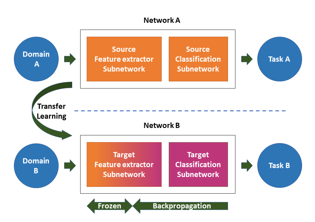
Figure 1: Illustration of a network based deep transfer learning from a source domain A and task A to target domain B and task B. The Network A is trained on a large training dataset and is called the pre-trained network. Network B is constructed by using parts of Network A followed by a new softmax classification network. Finally the resulting network B is initialized with the pre-trained weights and trained using backpropagation on the target dataset.

IV Experimental Setup

This section introduces the experimental setup in terms of the datasets, source CNN architectures, implementation and training details as well as the evaluation criteria. Also, the anomaly detection tasks are explained for every dataset.

IV-A Datasets

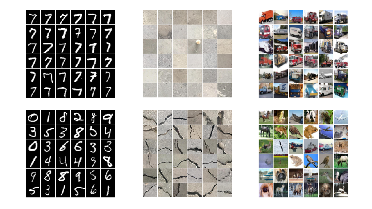
Figure 2: Exemplary images for the normal and anomaly classes for the MNIST [9], Cement Crack [10] and CIFAR10 [8] datasets from left to right.

In order to evaluate the proposed method and demonstrate its performance on the task of anomaly detection, experiments were conducted on three different datasets namely CIFAR10, MNIST and Concrete Crack. For the experiments conducted on CIFAR10 and MNIST the anomaly detection task was one versus the rest approach. The anomaly class consisted of one class from these datsets and the normal class was constructed using random sampling from the remaining nine classes with size equal to the normal class. The fact that the samples were drawn randomly from the rest of the classes as a whole introduces slight class imbalance and makes the anomaly detection more challenging. Concrete cracks have well defined normal and anomaly classes which are negative and positive crack classes respectively. Exemplary images for normal and anomalous classes for all the three datasets are shown in Fig. 2.

IV-A1 CIFAR10

This dataset consists of 60,000 32x32 colour images in 10 classes, with 6,000 images per class. There are 50,000 training images and 10000 test images. Using the leave-one-out approach ten different combinations of anomaly and normal classes were constructed. For each combination there were 5k training samples per class and 1k test samples per class.

IV-A2 MNIST

This dataset consists of 60,000 28x28 grayscale images of the 10 digits, along with a test set of 10,000 images. For this dataset too ten different combinations of anomaly and normal classes were constructed using the leave-one-out approach. For each combination there were 6k training samples per class and 1k test samples per class.

IV-A3 Concrete Crack

The dataset contains concrete images with two classes namely positive and negative crack. There are 20,000 277x277 color images for each class. Experiments were conducted with 2000 training images per class and 4,000 test images per class.

IV-B CNN architectures

Three state-of-the-art CNN architectures were selected for conducting experiments and are briefly described below.

IV-B1 DenseNet

Densely Connected Convolutional Networks [15] (DenseNets) are the latest addition to deep CNN architectures. Every layer is connected to every other layer in a feed forward fashion so that the network with L layers has $\frac{L(L+1)}{2}$ direct connections. DenseNet-169 architecture is used as the source network for our experiments.

IV-B2 ResNet

Deep Residual Networks [16] introduced the concept of identity shortcut connections that skip one or more layers. These were introduced in 2015 by Kaiming He. et.al. and bagged $1^{st}$ place in the ILSVRC 2015 classification competition . ResNet-152 architecture is used for the experiments.

IV-B3 Inception

Inception architectures were introduced by Google as GoogLeNet / Inception-v1. The basic building block inception module passes the input from previous layers through multiple convolution layers and max pooling simultaneously and are concatenated together at output. This eliminates the need to think of which filter size to use at each layer. Inception-V4 [17] architecture is used for the experiments.

IV-C Implementation

Publicly available implementations in Keras [18] of basic architecture and weights of these networks pre-trained on ImageNet were used as a starting point for all the three chosen architectures [19] [20]. As discussed in section III, after the model weights are loaded, the softmax layer is replaced with a new layer having two neurons for the anomaly detection task. Subsequently, the modified network is fine tuned by backpropagation.

For all the three networks following training parameters are the same. Stochastic gradient descent optimizer is used with parameters values as learning rate = $10^{-3}$, decay = $10^{-6}$, momentum = 0.9 and nesterov = true. Batch size is 16 and shuffling is enabled. The model is trained for 50 epochs and the best model is used for the results.

• DenseNet-169: The input images are resized to (224,224) before feeding the model.

• ResNet-152: The input images are resized to (224,224) before feeding the model.

• Inception-V4: The input images are resized to (299,299) before feeding the model.

The prediction probabilities from the normal class neuron are used as anomaly scores and for performing the anomaly detection evaluation.

For MNIST dataset RGB image is made by copying the greyscale values three times before re-sizing is performed.

IV-D Evaluation

Evaluation is done using the area under curve (AUC) measurement of the receiver operating characteristics (ROC) [21]. The ROC curve is plotted with true positive rates (TPR) against the false positive rates (FPR). ROC is a probability curve and AUC represents degree or measure of separability. An excellent model has AUC near to the 1 which means it has good measure of separability. When AUC is 0.5, it means the model has no class separation capacity whatsoever.

V Results and Discussion

AUC values of the experiments conducted for CIFAR10 and MNIST datasets are summarized in Table I and II respectively. The proposed method for all three chosen architectures clearly outperforms the previous work for the anomaly detection task across all the classes for both datasets. For the CIFAR10 dataset, the minimum, maximum and average improvement is 31%, 58% and 41%. Even for the deer class for which all the other methods perform poorly, an AUC value of 0.99 is obtained. For the MNIST dataset, an average increase of 20% is achieved over the other methods.

Table III summarizes the results on the cement crack which is a real world dataset. The GANomaly [4] model had to be trained on 16,000 samples to be able to achieve an AUC value of 0.858. Although for our transfer learning based approach all the three architectures were trained on only 2,000 images per class, the proposed method clearly outperforms by achieving an AUC value of 0.99.

The confusion matrices for the cement crack experiments are shown in Tables IV, V and VI. The architectures on an average have precision, recall and f1-score of 0.99, which indicates that the classifier is performing extremely well for the task of anomaly detection. Fig. 3 shows the examples that were miss-classified in the experiments. It is important to note here that in order to show the capability of the proposed approach despite fewer training examples, the architectures were trained only on 2,000 images per class. The results are better if more training data is available.

We see that even though all the three architectures achieve state-of-the-art results, there is variation among them. DenseNet-169 performs the best followed by ResNet-152 and finally Inception-V4. Even though on an average Inception-V4 performs lowest among the three architectures on the CIFAR10 dataset, it outperforms the other two on MNIST dataset. In the preliminary experiments conducted on the challenging German Asphalt Pavement Distress Dataset [22], DenseNet-169 achieved an average F1 score of 95% and AUC value of 0.91.

The stellar results achieved despite the low number of training examples using the challenging AUC evaluation metric on benchmark as well as real world datasets indicate that the proposed method is highly suitable for anomaly detection. The results also shown that it clearly outperforms the previous state-of-the-art methods.

TABLE I: AUC results for CIFAR10 dataset

	CIFAR10
Model	plane	car	bird	cat	deer	frog	horse	ship	truck	dog
GANomaly [4]	0.633	0.631	0.51	0.587	0.593	0.683	0.605	0.616	0.617	0.628
AnoGAN [3]	0.516	0.492	0.411	0.399	0.335	0.321	0.399	0.567	0.511	0.393
EGBAD [23]	0.577	0.514	0.383	0.448	0.374	0.353	0.526	0.413	0.555	0.481
DenseNet-169	0.998449	0.998933	0.994980	0.992014	0.998145	0.991758	0.999031	0.998386	0.998948	0.998291
ResNet-152	0.998071	0.998203	0.995249	0.991605	0.998480	0.991375	0.999607	0.999289	0.998934	0.997900
Inception-V4	0.930263	0.971474	0.842340	0.853591	0.895042	0.893674	0.949273	0.921899	0.954804	0.931945

TABLE II: AUC results for MNIST dataset

	MNIST
Model	Class 0	Class 1	Class 2	Class 3	Class 4	Class 5	Class 6	Class 7	Class 8	Class 9
GANomaly [4]	0.881	0.675	0.953	0.801	0.827	0.864	0.849	0.682	0.856	0.558
AnoGAN [3]	0.623	0.31	0.521	0.458	0.442	0.431	0.492	0.401	0.392	0.368
EGBAD [23]	0.783	0.294	0.523	0.506	0.453	0.436	0.593	0.398	0.523	0.358
DenseNet-169	0.998265	0.994258	0.984126	0.980750	0.983918	0.992295	0.984011	0.997476	0.991551	0.999386
ResNet-152	0.998050	0.994176	0.982025	0.981253	0.984338	0.989994	0.980970	0.998940	0.989815	0.998982
Inception-V4	0.997676	0.994609	0.983431	0.980548	0.984617	0.992676	0.983624	0.997108	0.994305	0.999080

TABLE III: AUC results for Concrete Crack dataset

Model	AUC
GANomaly [4]	0.858
DenseNet-169	0.999998
ResNet-152	0.999986
Inception-V4	0.998462

TABLE IV: Confusion Matrix for Concrete Crack dataset using DenseNet-169

		Predicted
		Crack	No Crack	Total
Actual	Crack	$3993$	$7$	$4000$
	No Crack	$0$	$4000$	$4000$
	Total	$3993$	$4007$	$8000$

TABLE V: Confusion Matrix for Concrete Crack dataset using ResNet-152

		Predicted
		Crack	No Crack	Total
Actual	Crack	$3975$	$25$	$4000$
	No Crack	$1$	$3999$	$4000$
	Total	$3976$	$4024$	$8000$

TABLE VI: Confusion Matrix for Concrete Crack dataset using Inception-V4

		Predicted
		Crack	No Crack	Total
Actual	Crack	$3952$	$48$	$4000$
	No Crack	$51$	$3949$	$4000$
	Total	$4003$	$3997$	$8000$

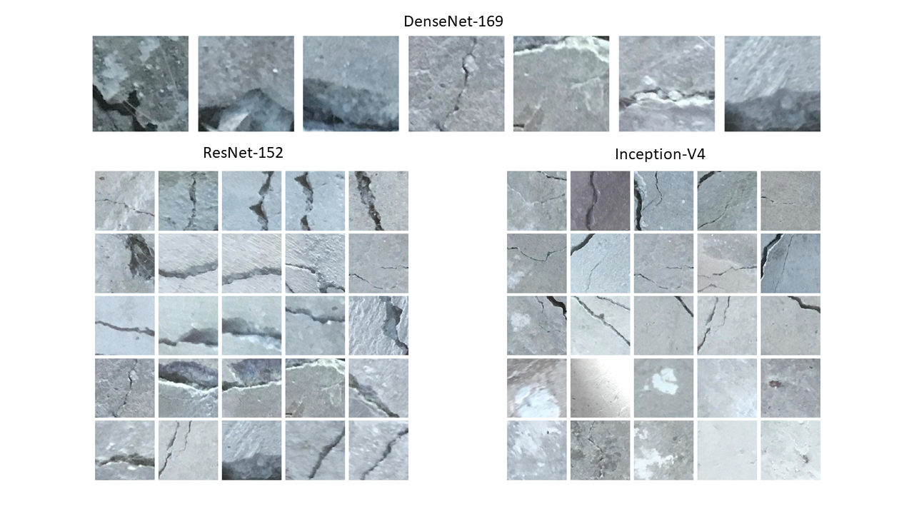
Figure 3: Few examples of miss-classified images for the Concrete Crack dataset for all the three architectures.

VI Conclusion

This paper introduces an approach that applies network-based deep transfer learning to the task of anomaly detection by treating it as a supervised binary classification problem. The quantitative results obtained on different datasets including a real world dataset show that the proposed technique achieves state-of-the-art results in comparison to existing techniques. The proposed method also addresses one of the most important challenges of anomaly detection which is the low availability of anomalous samples. This is demonstrated by the fact that the architectures were trained on low training samples per class and still the proposed method is able to separate the normal and abnormal classes competently. Future research can be conducted on the effect of source architecture choice, source dataset choice, effect of freezing first $n$ layers of the chosen architecture while training and the application of the method to other types of anomaly detection tasks.

References

- [1] V. Chandola, A. Banerjee, and V. Kumar, “Anomaly detection: A survey,” ACM Comput. Surv., vol. 41, no. 3, pp. 15:1–15:58, Jul. 2009. [Online]. Available: http://doi.acm.org/10.1145/1541880.1541882
- [2] Y. Lu and P. Xu, “Anomaly detection for skin disease images using variational autoencoder,” CoRR, vol. abs/1807.01349, 2018.
- [3] T. Schlegl, P. Seeböck, S. M. Waldstein, U. Schmidt-Erfurth, and G. Langs, “Unsupervised anomaly detection with generative adversarial networks to guide marker discovery,” in Information Processing in Medical Imaging, M. Niethammer, M. Styner, S. Aylward, H. Zhu, I. Oguz, P.-T. Yap, and D. Shen, Eds. Cham: Springer International Publishing, 2017, pp. 146–157.
- [4] S. Akcay, A. A. Abarghouei, and T. P. Breckon, “Ganomaly: Semi-supervised anomaly detection via adversarial training,” CoRR, vol. abs/1805.06725, 2018.
- [5] B. Barz, E. Rodner, Y. G. Garcia, and J. Denzler, “Detecting regions of maximal divergence for spatio-temporal anomaly detection,” IEEE Transactions on Pattern Analysis and Machine Intelligence, pp. 1–1, 2018.
- [6] M. A. F. Pimentel, D. A. Clifton, L. Clifton, and L. Tarassenko, “Review: A review of novelty detection,” Signal Process., vol. 99, pp. 215–249, Jun. 2014. [Online]. Available: http://dx.doi.org/10.1016/j.sigpro.2013.12.026
- [7] N. Görnitz, M. Kloft, K. Rieck, and U. Brefeld, “Toward supervised anomaly detection,” J. Artif. Int. Res., vol. 46, no. 1, pp. 235–262, Jan. 2013. [Online]. Available: http://dl.acm.org/citation.cfm?id=2512538.2512545
- [8] A. Krizhevsky, V. Nair, and G. Hinton, “Cifar-10 (canadian institute for advanced research).” [Online]. Available: http://www.cs.toronto.edu/ kriz/cifar.html
- [9] Y. LeCun and C. Cortes, “MNIST handwritten digit database,” 2010. [Online]. Available: http://yann.lecun.com/exdb/mnist/
- [10] “Concrete crack images for classification, mendeley data, v1.” [Online]. Available: http://dx.doi.org/10.17632/5y9wdsg2zt.1
- [11] C. Tan, F. Sun, T. Kong, W. Zhang, C. Yang, and C. Liu, “A survey on deep transfer learning.” in ICANN 2018, 2018.
- [12] L. Torrey and J. W. Shavlik, “Transfer learning,” 2009.
- [13] A. Karpathy, “Stanford University CS231n: Convolutional Neural Networks for Visual Recognition.” [Online]. Available: http://cs231n.stanford.edu/syllabus.html
- [14] J. Huang, J. Li, D. Yu, L. Deng, and Y. Gong, “Cross-language knowledge transfer using multilingual deep neural network with shared hidden layers,” in 2013 IEEE International Conference on Acoustics, Speech and Signal Processing, May 2013, pp. 7304–7308.
- [15] G. Huang, Z. Liu, L. van der Maaten, and K. Q. Weinberger, “Densely connected convolutional networks,” 2017 IEEE Conference on Computer Vision and Pattern Recognition (CVPR), pp. 2261–2269, 2017.
- [16] K. He, X. Zhang, S. Ren, and J. Sun, “Deep residual learning for image recognition,” 2016 IEEE Conference on Computer Vision and Pattern Recognition (CVPR), pp. 770–778, 2016.
- [17] C. Szegedy, S. Ioffe, and V. Vanhoucke, “Inception-v4, inception-resnet and the impact of residual connections on learning,” in AAAI, 2017.
- [18] F. Chollet et al., “Keras,” https://keras.io, 2015.
- [19] K. Team, “Keras applications,” Jan 2019. [Online]. Available: https://github.com/keras-team/keras-applications/tree/master/keras_applications
- [20] Kentsommer, “Keras inception-v4,” Sep 2017. [Online]. Available: https://github.com/kentsommer/keras-inceptionV4
- [21] C. X. Ling, J. Huang, and H. Zhang, “Auc: A statistically consistent and more discriminating measure than accuracy,” in Proceedings of the 18th International Joint Conference on Artificial Intelligence, ser. IJCAI’03. San Francisco, CA, USA: Morgan Kaufmann Publishers Inc., 2003, pp. 519–524. [Online]. Available: http://dl.acm.org/citation.cfm?id=1630659.1630736
- [22] M. Eisenbach, R. Stricker, D. Seichter, K. Amende, K. Debes, M. Sesselmann, D. Ebersbach, U. Stoeckert, and H.-M. Gross, “How to get pavement distress detection ready for deep learning? a systematic approach.” in International Joint Conference on Neural Networks (IJCNN), 2017, pp. 2039–2047.
- [23] H. Zenati, C. S. Foo, B. Lecouat, G. Manek, and V. R. Chandrasekhar, “Efficient gan-based anomaly detection,” CoRR, vol. abs/1802.06222, 2018.