Threshold Regression with Nonparametric Sample Splitting

Abstract

This paper develops a threshold regression model where an unknown relationship between two variables nonparametrically determines the threshold. We allow the observations to be cross-sectionally dependent so that the model can be applied to determine an unknown spatial border for sample splitting over a random field. We derive the uniform rate of convergence and the nonstandard limiting distribution of the nonparametric threshold estimator. We also obtain the root-n consistency and the asymptotic normality of the regression coefficient estimator. Our model has broad empirical relevance as illustrated by estimating the tipping point in social segregation problems as a function of demographic characteristics; and determining metropolitan area boundaries using nighttime light intensity collected from satellite imagery. We find that the new empirical results are substantially different from those in the existing studies.

Keywords: threshold regression, sample splitting, nonparametric, random field, tipping point, metropolitan area boundary.

JEL Classifications: C14, C21, C24, R1

1 Introduction

Sample splitting and threshold regression models have spawned a vast literature in econometrics and statistics. Existing studies typically specify the sample splitting criteria in a parametric way as whether a single random variable or a linear combination of variables crosses some unknown threshold. See, for example, Hansen (2000), Caner and Hansen (2004), Seo and Linton (2007), Lee, Seo, and Shin (2011), Li and Ling (2012), Yu (2012), Lee, Liao, Seo, and Shin (2020), Hidalgo, Lee, and Seo (2019), and Yu and Fan (2020). In this paper, we study a novel extension to consider a nonparametric sample splitting model. Such an extension leads to new theoretical results and substantially generalizes the empirical applicability of threshold models.

Specifically, we consider a model given by

$$y_{i}=x_{i}^{\top}\beta_{0}+x_{i}^{\top}\delta_{0}\mathbf{1}\left[q_{i}\leq\gamma_{0}\left(s_{i}\right)\right]+u_{i}$$ (1)

for $i=1,\ldots,n$, where $\mathbf{1}\left[\cdot\right]$ is the binary indicator. In this model, the marginal effect of $x_{i}$ to $y_{i}$ can be different across $i$ as $(\beta_{0}+\delta_{0})$ or $\beta_{0}$ depending on whether $q_{i}\leq\gamma_{0}\left(s_{i}\right)$ or not. The threshold function $\gamma_{0}(\cdot)$ is unknown, and the main parameters of interest are $\beta_{0}$, $\delta_{0}$, and $\gamma_{0}(\cdot)$. The novel feature of this model is that the sample splitting is determined by an unknown relationship between two variables $q_{i}$ and $s_{i}$, and their relationship is characterized by the nonparametric threshold function $\gamma_{0}(\cdot)$. In contrast, the classical threshold regression models assume $\gamma_{0}\left(\cdot\right)$ to be a constant or a linear index. Our new specification can cover interesting cases that have not been studied. For example, we can consider the threshold to be heterogeneous and specific to each observation $i$ if we see $\gamma_{0}\left(s_{i}\right)=\gamma_{0i}$; or the threshold to be determined by the direction of some moment condition $\gamma_{0}(s_{i})=\mathbb{E}[q_{i}|s_{i}]$. Apparently, when $\gamma_{0}(s)=\gamma_{0}$ or $\gamma_{0}(s)=\gamma_{0}s$ for some parameter $\gamma_{0}$ and $s\neq 0$, it reduces to the standard threshold regression model.

The new model is motivated by the following two applications: estimating potentially heterogeneous thresholds in public economics and determining spatial sample splitting in urban economics. The first one is about the tipping point model proposed by Schelling (1971), who analyzes the phenomenon that a neighborhood’s white population substantially decreases once the minority share exceeds a certain threshold, called the tipping point. Card, Mas, and Rothstein (2008) empirically estimate the tipping point model by considering the constant threshold regression, $y_{i}=\beta_{10}+\delta_{10}\mathbf{1}\left[q_{i}\leq\gamma_{0}\right]+x_{2i}^{\top}\beta_{20}+u_{i}$, where $y_{i}$ is the white population change in a decade and $q_{i}$ is the initial minority share in the $i$th tract. The parameters $\delta_{10}$ and $\gamma_{0}$ denote the change size and the threshold, respectively. In Section VII of Card, Mas, and Rothstein (2008), however, they find that the tipping point $\gamma_{0}$ varies depending on the attitudes of white residents toward the minority. This finding raises the concern on the constant threshold model and motivates us to study the more general model (1) by specifying the tipping point $\gamma_{0}$ as a nonparametric function of local demographic characteristics. We estimate such a tipping function in Section 6.1.

For the second application, we use the model (1) to define metropolitan area boundaries, which is a fundamental problem in urban economics. Recently, many studies propose to use nighttime light intensity collected from satellite imagery to define the metropolitan area. They set an ad hoc level of light intensity as a threshold and categorize a pixel in the satellite imagery as a part of the metropolitan area if the light intensity of that pixel is higher than the threshold. See, for example, Rozenfeld, Rybski, Gabaix, and Makse (2011), Henderson, Storeygard, and Weil (2012), Dingel, Miscio, and Davis (2019), and Vogel, Goldblatt, Hanson, and Khandelwal (2019). In contrast, the model (1) can provide a data-driven guidance of choosing the intensity threshold from the econometric perspective, if we let $y_{i}$ as the light intensity in the $i$th pixel and $(q_{i},s_{i})$ as the location information of that pixel (more precisely, the coordinate of a point on a rotated map as described in Section 4). In Section 6.2, we estimate the metropolitan area of Dallas, Texas, especially its development from 1995 to 2010, and find substantially different results from the conventional approaches. To the best of our knowledge, this is the first study to nonparametrically determine the metropolitan area using a threshold model.

We develop a two-step estimation procedure of (1), where we estimate $\gamma_{0}\left(\cdot\right)$ by the local constant least squares. Under the shrinking threshold asymptotics as in Bai (1997), Bai and Perron (1998), and Hansen (2000), we show that the nonparametric estimator $\widehat{\gamma}(\cdot)$ is uniformly consistent and has a highly nonstandard limiting distribution. Based on such distribution, we develop a pointwise specification test of $\gamma_{0}(s)$ for any given $s$, which enables us to construct a confidence interval by inverting the test. Besides, the parametric part $(\widehat{\beta}^{\top},\widehat{\delta}^{\top})^{\top}$ is shown to satisfy the root-$n$ asymptotic normality.

We highlight some novel technical features of the new estimator as follows. First, since the nonparametric function $\gamma_{0}\left(\cdot\right)$ is inside the indicator function, technical proofs of the asymptotic results are non-standard. In particular, we establish the uniform rate of convergence of $\widehat{\gamma}\left(\cdot\right)$, which involves substantially more complicated derivations than the standard (constant) threshold regression model. Second, we find that, unlike the standard kernel estimator, $\widehat{\gamma}(\cdot)$ is asymptotically unbiased even if the optimal bandwidth is used. Also, when the change size $\delta_{0}$ shrinks very slowly, the optimal rate of convergence of $\widehat{\gamma}(\cdot)$ becomes close to the root-$n$ rate. In the standard kernel regression, such a fast rate of convergence can be obtained when the unknown function is infinitely differentiable, while we only require the second-order differentiability of $\gamma_{0}\left(\cdot\right)$. Third, to limit the effect of estimating $\gamma_{0}\left(\cdot\right)$ to $(\widehat{\beta}^{\top},\widehat{\delta}^{\top})^{\top}$, we propose to use the observations that are sufficiently away from the estimated threshold in the second-step parametric estimation. The choice of this distance is obtained by the uniform convergence rate of $\widehat{\gamma}\left(\cdot\right)$. Fourth, we let the variables be cross-sectionally dependent by considering the strong-mixing random field as in Conley (1999) and Conley and Molinari (2007). This generalization allows us to study nonparametric sample splitting of spatial observations. For instance, if we let $(q_{i},s_{i})$ correspond to the geographical location (i.e., latitude and longitude on the map), then the threshold $\mathbf{1}\left[q_{i}\leq\gamma_{0}\left(s_{i}\right)\right]$ identifies the unknown border yielding a two-dimensional sample splitting. In more general contexts, the model can be applied to identify social or economic segregation over interacting agents. Finally, noting that $\mathbf{1}\left[q_{i}\leq\gamma_{0}\left(s_{i}\right)\right]$ can be considered as the special case of $\mathbf{1}\left[g_{0}\left(q_{i},s_{i}\right)\leq 0\right]$ when $g_{0}$ is monotonically increasing in $q_{i}$, we discuss how to extend the proposed method to such a more general case that leads to a threshold contour model.

The rest of the paper is organized as follows. Section 2 sets up the model, establishes the identification, and defines the estimator. Section 3 derives the asymptotic properties of the estimators and develops a likelihood ratio test of the threshold function. Section 4 describes how to extend the main model to estimate a threshold contour. Section 5 studies small sample properties of the proposed statistics by Monte Carlo simulations. Section 6 applies the new method to estimate the tipping point function and to determine metropolitan areas. Section 7 concludes this paper with some remarks. The main proofs are in the Appendix, and all the omitted proofs are collected in the supplementary material.

We use the following notations. Let $\rightarrow_{p}$ denote convergence in probability, $\rightarrow_{d}$ convergence in distribution, and $\Rightarrow$ weak convergence of the underlying probability measure as $n\rightarrow\infty$. Let $\left\lfloor r\right\rfloor$ denote the biggest integer smaller than or equal to $r$, $\mathbf{1}[E]$ the indicator function of a generic event $E$, and $\left\|A\right\|$ the Euclidean norm of a vector or matrix $A$. For any set $B$, let $|B|$ as the cardinality of $B$.

2 Model Setup

We assume spatial processes located on an evenly spaced lattice $\Lambda\subset\mathbb{R}^{2}$, following Conley (1999), Conley and Molinari (2007), and Carbon, Francq, and Tran (2007). We consider the threshold regression model given by (1), which is

$$y_{i}=x_{i}^{\top}\beta_{0}+x_{i}^{\top}\delta_{0}\mathbf{1}\left[q_{i}\leq\gamma_{0}\left(s_{i}\right)\right]+u_{i}\text{,}$$

where the observations $\{(y_{i},x_{i}^{\top},q_{i},s_{i})^{\top}\in\mathbb{R}^{1+\dim(x)+1+1};i\in\Lambda_{n}\}$ are a triangular array of real random variables defined on some probability space with $\Lambda_{n}$ being a fixed sequence of finite subsets of $\Lambda$. In this setup, the cardinality of $\Lambda_{n}$, $n=|\Lambda_{n}|$, is the sample size and $\sum_{i\in\Lambda_{n}}$ denotes the summation of all observations. For readability, we postpone the regularity conditions on $\Lambda_{n}$ in Assumption A later. The threshold function $\gamma_{0}:\mathbb{R\rightarrow R}$ as well as the regression coefficients $\theta_{0}=(\beta_{0}^{\top},\delta_{0}^{\top})^{\top}\in\mathbb{R}^{2\dim(x)}$ are unknown, and they are the parameters of interest. Since we consider a shrinking threshold effect, the parameter $\delta_{0}$ is to depend on the sample size $n$ as in Assumption A-(ii) below; hence $\delta_{0}$ and $\theta_{0}$ should be written as $\delta_{n0}$ and $\theta_{n0}$, respectively. However, we write $\delta_{0}$ and $\theta_{0}$ for simplicity. We let $\mathcal{Q}\subset\mathbb{R}$ and $\mathcal{S}\subset\mathbb{R}$ denote the supports of $q_{i}$ and $s_{i}$, respectively. Suppose the space of $\gamma_{0}\left(s\right)$ for any $s$ is a compact set $\Gamma\subset\mathbb{R}$.

First, we establish the identification, which requires the following conditions.

Assumption ID

(i) $\mathbb{E}\left[u_{i}|x_{i},q_{i},s_{i}\right]=0$ almost surely.

(ii) $\mathbb{E}\left[x_{i}x_{i}^{\top}\right]>\mathbb{E}\left[x_{i}x_{i}^{\top}\mathbf{1}\left[q_{i}\leq\gamma\right]\right]>0$ for any $\gamma\in\Gamma$.

(iii) For any $s\in\mathcal{S}$, there exists $\varepsilon(s)>0$ such that $\varepsilon(s)<\mathbb{P}\left(q_{i}\leq\gamma_{0}(s_{i})|s_{i}=s\right)<1-\varepsilon(s)$ and $\delta_{0}^{\top}\mathbb{E}\left[x_{i}x_{i}^{\top}|q_{i}=q,s_{i}=s\right]\delta_{0}>0$ for all $\left(q,s\right)\in\mathcal{Q}\times\mathcal{S}$.

(iv) $q_{i}$ is continuously distributed with its conditional density $f(q|s)$ satisfying that $0<C_{1}<f(q|s)<C_{2}<\infty$ for all $\left(q,s\right)\in\Gamma\times\mathcal{S}$ and some constants $C_{1}$ and $C_{2}$.

Assumption ID is mild. The condition (i) excludes endogeneity, and (ii) is the full rank condition to identify the global parameters $\beta_{0}$ and $\delta_{0}$. The conditions (ii) and (iii) require that the location of the threshold is not on the boundary of the support of $q_{i}$ for any $s\in\mathcal{S}$, which is inevitable for identification and has been commonly assumed in the existing threshold literature (e.g., Hansen (2000)). If $\gamma_{0}(s)$ reaches the boundary of $q_{i}$ for some $s\in\mathcal{S}$, then no observation can be generated from one side of the threshold function at this $s$, and identification is failed. The second condition in (iii) assumes the coefficient change exists (i.e., $\delta_{0}\neq 0$). Note that it does not require $\mathbb{E}\left[x_{i}x_{i}^{\top}|q_{i}=q,s_{i}=s\right]$ to be of full rank, and hence $q_{i}$ or $s_{i}$ can be one of the elements of $x_{i}$ (e.g., the threshold autoregressive model by Tong (1983)) or a linear combination of $x_{i}$. The condition (iv) requires the conditional density of $q_{i}$ given any $s_{i}$ is positive and bounded in $\Gamma$.

Under Assumption ID, the following theorem establishes the identification of the semiparametric threshold regression model (1).

Theorem 1

Under Assumption ID, the parameters $(\beta_{0}^{\top},\delta_{0}^{\top})^{\top}$ are the unique minimizer of $\mathbb{E}[(y_{i}-x_{i}^{\top}\beta-x_{i}^{\top}\delta\mathbf{1}\left[q_{i}\leq\gamma\right])^{2}]$ for any $\gamma\in\Gamma$, and the threshold function $\gamma_{0}\left(s\right)$ is the unique minimizer of $\mathbb{E}[(y_{i}-x_{i}^{\top}\beta_{0}-x_{i}^{\top}\delta_{0}\mathbf{1}\left[q_{i}\leq\gamma(s_{i})\right])^{2}|s_{i}=s]$ for each given $s\in\mathcal{S}$.

Given identification, we proceed to estimate this semiparametric model in two steps. First, for given $s\in\mathcal{S}$, we fix $\gamma_{0}(s)=\gamma$ and obtain $\widehat{\beta}\left(\gamma;s\right)$ and $\widehat{\delta}\left(\gamma;s\right)$ by the local constant least squares conditional on $\gamma$:

$$(\widehat{\beta}\left(\gamma;s\right)^{\intercal},\widehat{\delta}\left(\gamma;s\right)^{\intercal})^{\intercal}=\arg\min_{\beta,\delta}Q_{n}\left(\beta,\delta,\gamma;s\right)\text{,}$$ (2)

where

$$Q_{n}\left(\beta,\delta,\gamma;s\right)=\mathop{\displaystyle\sum}_{i\in\Lambda_{n}}K\left(\frac{s_{i}-s}{b_{n}}\right)\left(y_{i}-x_{i}^{\top}\beta-x_{i}^{\top}\delta\mathbf{1}\left[q_{i}\leq\gamma\right]\right)^{2}$$ (3)

for some kernel function $K\left(\cdot\right)$ and a bandwidth parameter $b_{n}$. Then $\gamma_{0}(s)$ is estimated by

$$\widehat{\gamma}\left(s\right)=\arg\min_{\gamma\in\Gamma_{n}}Q_{n}\left(\gamma;s\right)$$ (4)

for given $s$, where $\Gamma_{n}=\Gamma\cap\{q_{1},\ldots,q_{n}\}$ and $Q_{n}\left(\gamma;s\right)$ is the concentrated sum of squares defined as

$$Q_{n}\left(\gamma;s\right)=Q_{n}\left(\widehat{\beta}\left(\gamma;s\right),\widehat{\delta}\left(\gamma;s\right),\gamma;s\right)\text{.}$$ (5)

To avoid any additional technical complexity, we focus on estimation of $\gamma_{0}(s)$ at $s\in\mathcal{S}_{0}\subset\mathcal{S}$ for some compact interior subset $\mathcal{S}_{0}$ of the support, say the middle 70% quantiles. Note that, given $s$, the nonparametric estimator $\widehat{\gamma}\left(s\right)$ can be seen as a local version of the standard (constant) threshold regression estimator. Therefore, the computation of (4) requires one-dimensional grid search of the threshold for only $n$ times as in the standard threshold regression estimation.

In the second step, we estimate the parametric components $\beta_{0}$ and $\delta_{0}$. To minimize any potential effects from the first step estimation, we estimate $\beta_{0}$ and $\delta_{0}^{\ast}=\beta_{0}+\delta_{0}$ using the observations that are sufficiently away from the estimated threshold. This is implemented by considering

$$\widehat{\beta} = \arg\min_{\beta}\mathop{\displaystyle\sum}_{i\in\Lambda_{n}}\left(y_{i}-x_{i}^{\top}\beta\right)^{2}\mathbf{1}\left[q_{i}>\widehat{\gamma}\left(s_{i}\right)+\pi_{n}\right]\mathbf{1}[s_{i}\in\mathcal{S}_{0}]\text{,}$$ (6)

$$\widehat{\delta}^{\ast} = \arg\min_{\delta^{\ast}}\mathop{\displaystyle\sum}_{i\in\Lambda_{n}}\left(y_{i}-x_{i}^{\top}\delta^{\ast}\right)^{2}\mathbf{1}\left[q_{i}<\widehat{\gamma}\left(s_{i}\right)-\pi_{n}\right]\mathbf{1}[s_{i}\in\mathcal{S}_{0}]$$ (7)

for some constant $\pi_{n}>0$ satisfying $\pi_{n}\rightarrow 0$ as $n\rightarrow\infty$, which is defined later. The change size $\delta$ can be estimated as $\widehat{\delta}=\widehat{\delta}^{\ast}-\widehat{\beta}$.

For the asymptotic behavior of the threshold estimator, the existing literature typically assumes martingale difference arrays (e.g., Hansen (2000) and Lee, Liao, Seo, and Shin (2020)) or random samples (e.g., Yu (2012) and Yu and Fan (2020)). In this paper, we allow for cross-sectional dependence by considering spatial $\alpha$-mixing processes as in Bolthausen (1982) and Conley (1999). More precisely, for any indices (or locations) $i,j\in\Lambda$, we define the metric $\lambda\left(i,j\right)=\max_{1\leq\ell\leq\dim\left(\Lambda\right)}\left|i_{\ell}-j_{\ell}\right|$ and the corresponding norm $\max_{1\leq\ell\leq\dim\left(\Lambda\right)}\left|i_{\ell}\right|$, where $i_{\ell}$ denotes the $\ell$th component of $i$. The distance of any two subsets $\Lambda_{1},\Lambda_{2}\subset\Lambda$ is defined as $\lambda(\Lambda_{1},\Lambda_{2})=\inf\{\lambda(i,j):i\in\Lambda_{1},j\in\Lambda_{2}\}$. We let $\mathcal{F}_{\Lambda}$ be the $\sigma$-algebra generated by a random sequence $\left(x_{i}^{\top},q_{i},s_{i},u_{i}\right)^{\top}$ for $i\in\Lambda$ and define the spatial $\alpha$-mixing coefficient as

$$\alpha_{k,l}(m)=\sup\left\{\left|\mathbb{P}\left(A\cap B\right)-\mathbb{P}\left(A\right)\mathbb{P}\left(B\right)\right|:A\in\mathcal{F}_{\Lambda_{1}}\text{, }B\in\mathcal{F}_{\Lambda_{2}}\text{, }\lambda\left(\Lambda_{1},\Lambda_{2}\right)\geq m\right\}\text{,}$$ (8)

where $\left|\Lambda_{1}\right|\leq k$ and $\left|\Lambda_{2}\right|\leq l$. Without loss of generality, we assume $\alpha_{k,l}(0)=1$ and $\alpha_{k,l}(m)$ is monotonically decreasing in $m$ for all $k$ and $l$.

The following conditions are imposed for deriving the asymptotic properties of our two-step estimator. Let $f\left(q,s\right)$ be the joint density function of $(q_{i},s_{i})$ and

$$D\left(q,s\right) = \mathbb{E}[x_{i}x_{i}^{\top}|\left(q_{i},s_{i}\right)=\left(q,s\right)]\text{,}$$ (9)

$$V\left(q,s\right) = \mathbb{E}[x_{i}x_{i}^{\top}u_{i}^{2}|\left(q_{i},s_{i}\right)=\left(q,s\right)]\text{.}$$ (10)

Assumption A

(i) The lattice $\Lambda_{n}\subset\mathbb{R}^{2}$ is infinitely countable; all the elements in $\Lambda_{n}$ are located at distances at least $\lambda_{0}>1$ from each other (i.e., for any $i,j\in\Lambda_{n}$, $\lambda\left(i,j\right)\geq\lambda_{0}$); and $\lim_{n\rightarrow\infty}\left|\partial\Lambda_{n}\right|/n=0$, where $\partial\Lambda_{n}=\{i\in\Lambda_{n}:\exists j\not\in\Lambda_{n}$ with $\lambda(i,j)=1\}$.

(ii) $\delta_{0}=c_{0}n^{-\epsilon}$ for some $c_{0}\neq 0$ and $\epsilon\in(0,1/2)$; $\left(c_{0}^{\top},\beta_{0}^{\top}\right)^{\top}$ belongs to some compact subset of $\mathbb{R}^{2\dim(x)}$.

(iii) $\left(x_{i}^{\top},q_{i},s_{i},u_{i}\right)^{\top}$ is strictly stationary and $\alpha$-mixing with the mixing coefficient $\alpha_{k,l}(m)$ defined in (8), which satisfies that for all $k$ and $l$, $\alpha_{k,l}(m)\leq C_{1}\exp(-C_{2}m)$ for some positive constants $C_{1}$ and $C_{2}$.

(iv) $0<\mathbb{E}\left[u_{i}^{2}|x_{i},q_{i},s_{i}\right]<\infty$ almost surely.

(v) Uniformly in $\left(q,s\right)$, there exist some finite constants $\varphi>0$ and $C>0$ such that $\mathbb{E}[||x_{i}x_{i}^{\top}||^{4+\varphi}|(q_{i},s_{i})=(q,s)]<C$ and $\mathbb{E}[||x_{i}u_{i}||^{4+\varphi}|(q_{i},s_{i})=(q,s)]<C$.

(vi) $\gamma_{0}:\mathcal{S}\mapsto\Gamma$ is a twice continuously differentiable function with bounded derivatives.

(vii) $D\left(q,s\right)$, $V\left(q,s\right)$, and $f\left(q,s\right)$ are uniformly bounded in $(q,s)$, continuous in $q$, and twice continuously differentiable in $s$ with bounded derivatives. For any $i,j\in\Lambda_{n}$, the joint density of $(q_{i},q_{j},s_{i},s_{j})^{\intercal}$ is uniformly bounded above by some constant $C<\infty$ and continuously differentiable in all components.

(viii) $c_{0}^{\top}D\left(\gamma_{0}(s),s\right)c_{0}>0$, $c_{0}^{\top}V\left(\gamma_{0}(s),s\right)c_{0}>0$, and $f\left(\gamma_{0}(s),s\right)>0$ for all $s\in\mathcal{S}$.

(ix) As $n\rightarrow\infty$, $b_{n}\rightarrow 0$, $n^{1-2\epsilon}b_{n}/\log n\rightarrow\infty$, $\log n/(nb_{n}^{2})\rightarrow 0$, and $nb_{n}^{(2+2\varphi)/(2+\varphi)}\rightarrow\infty$ for some $\varphi>0$ given in (v).

(x) $K\left(\cdot\right)$ is a positive second-order kernel, which is Lipschitz, symmetric around zero, and nonincreasing on $\mathbb{R}^{+}$ and satisfies $\int K\left(v\right)dv=1$, $\int v^{2}K\left(v\right)dv<\infty$.

We provide some discussions about Assumption A. First, we assume that $q_{i}$ and $s_{i}$ are continuous random variables as in the example in Section 6.1. This setup also covers the two-dimensional “spatial structural break” model as a special case as in the example in Section 6.2. For the latter case, we denote $n_{1}$ and $n_{2}$ as the numbers of rows (latitudes) and columns (longitudes) in the grid of pixels, and normalize $q$ and $s$ in the way that $q\in\{1/n_{1},2/n_{1},\ldots,1\}$ and $s\in\{1/n_{2},2/n_{2},\ldots,1\}$. Under similar (and even weaker) regularity conditions as Assumption A, we can show that the asymptotic results in the following sections extend to this case once we treat $(q_{i},s_{i})^{\top}$ as independently and uniformly distributed random variables over $\left[0,1\right]^{2}$. Such similarity is also found in the standard structural break and the threshold regression models (e.g., Proposition 5 in Bai and Perron (1998) and Theorem 1 in Hansen (2000)).

Second, Assumption A is mild and common in the existing literature. In particular, the condition (i) is the same as in Bolthausen (1982) to define the latent random field. Note that $\lambda_{0}$ can be any strictly positive value, and hence we can impose $\lambda_{0}>1$ without loss of generality. The condition (ii) adopts the widely used shrinking change size setup as in Bai (1997), Bai and Perron (1998), and Hansen (2000) to obtain a simple limiting distribution. In contrast, a constant change size (when $\epsilon=0$) leads to a complicated asymptotic distribution of the threshold estimator, which depends on nuisance parameters (e.g., Chan (1993)). The condition (iii) is required to establish the maximal inequality and uniform convergence in a spatially dependent random field. We impose a stronger condition than Jenish and Prucha (2009) to obtain the maximal inequality uniformly over $\gamma$ and $s$. We could weaken this condition such that $\alpha_{k,l}(m)$ decays at a polynomial rate (e.g., $\alpha_{k,l}(m)\leq Cm^{-r}$ for some $r>8$ and a constant $C$ as in Carbon, Francq, and Tran (2007)) if we impose higher moment restrictions in the condition (v). However, this exponential decay rate simplifies the technical proofs. The conditions (iv) to (viii) are similar to Assumption 1 of Hansen (2000). The condition (ix) imposes restrictions on the bandwidth $b_{n}$, which now depends on $\epsilon$ and $\varphi$. The condition (x) holds for many commonly used kernel functions including the Gaussian and the uniform kernels.

Third, we assume $\gamma_{0}\left(\cdot\right)$ to be a function from $\mathcal{S}$ to $\Gamma$ in Assumption A-(vi), which is not necessarily one-to-one. For this reason, sample splitting based on $\mathbf{1}\left[q_{i}\leq\gamma_{0}\left(s_{i}\right)\right]$ can be different from that based on $\mathbf{1}\left[s_{i}\geq\breve{\gamma}_{0}\left(q_{i}\right)\right]$ for some function $\breve{\gamma}_{0}\left(\cdot\right)$. Instead of restricting $\gamma_{0}\left(\cdot\right)$ to be one-to-one in this paper, we presume that one knows which variables should be respectively assigned as $q_{i}$ and $s_{i}$ from the context. Alternatively, we can consider a function $g_{0}\left(q,s\right)$ such that $g_{0}$ is monotonically increasing in $q$ for any $s$. Then, $\mathbf{1}\left[q_{i}\leq\gamma_{0}\left(s_{i}\right)\right]$ is viewed as a special case of $\mathbf{1}\left[g_{0}\left(q_{i},s_{i}\right)\leq 0\right]$ by inverting $g_{0}\left(\cdot,s\right)=q^{\ast}$, where $g_{0}\left(q^{\ast},s\right)=0$. We discuss such extension to identify a threshold contour in Section 4.

3 Asymptotic Results

We first obtain the asymptotic properties of $\widehat{\gamma}\left(s\right)$. The following theorem derives the pointwise consistency and the pointwise rate of convergence of $\widehat{\gamma}\left(s\right)$ at the interior points of $\mathcal{S}$.

Theorem 2

For a given $s\in\mathcal{S}_{0}$, under Assumptions ID and A, $\widehat{\gamma}\left(s\right)\rightarrow_{p}\gamma_{0}\left(s\right)$ as $n\rightarrow\infty$. Furthermore,

$$\widehat{\gamma}\left(s\right)-\gamma_{0}\left(s\right)=O_{p}\left(\frac{1}{n^{1-2\epsilon}b_{n}}\right)$$ (11)

provided that $n^{1-2\epsilon}b_{n}^{2}$ does not diverge.

The pointwise rate of convergence of $\widehat{\gamma}\left(s\right)$ depends on two parameters, $\epsilon$ and $b_{n}$. It is decreasing in $\epsilon$ like the parametric (constant) threshold case: a larger $\epsilon$ reduces the threshold effect $\delta_{0}=c_{0}n^{-\epsilon}$ and hence decreases the effective sampling information on the threshold. Since we estimate $\gamma_{0}(\cdot)$ using the kernel estimation method, the rate of convergence depends on the bandwidth $b_{n}$ as well. As in the standard kernel estimator case, a smaller bandwidth decreases the effective local sample size, which reduces the precision of the estimator $\widehat{\gamma}\left(s\right)$. Therefore, in order to have a sufficiently fast rate of convergence, we need to choose $b_{n}$ large enough when the threshold effect $\delta_{0}$ is expected to be small (i.e., when $\epsilon$ is close to $1/2$).

Unlike the standard kernel estimator, there seems no bias-variance trade-off in $\widehat{\gamma}\left(s\right)$ in (11), implying that we could improve the rate of convergence by choosing a larger bandwidth $b_{n}$. However, as we can find in Theorem 3 below, $b_{n}$ cannot be chosen too large to result in $n^{1-2\epsilon}b_{n}^{2}\rightarrow\infty$, under which $n^{1-2\epsilon}b_{n}(\widehat{\gamma}\left(s\right)-\gamma_{0}\left(s\right))$ is no longer $O_{p}(1)$. Therefore, we can obtain the optimal bandwidth using the restriction that $n^{1-2\epsilon}b_{n}^{2}$ does not diverge.

Under this restriction, we find the optimal bandwidth as $b_{n}^{\ast}=n^{-(1-2\epsilon)/2}c^{\ast}$ for some constant $0<c^{\ast}<\infty$, which yields the optimal pointwise rate of convergence of $\widehat{\gamma}\left(s\right)$ as $n^{-(1-2\epsilon)/2}$. However, such a bandwidth choice is not feasible because of the unknown constant $c^{\ast}$ and the nuisance parameter $\epsilon$ that are not estimable. In practice, we suggest cross validation as we implement in Section 6, although its statistical properties need to be studied further. Note that, when the change size $\delta_{0}$ shrinks very slowly with $n$ (i.e., $\epsilon$ is close to $0$), the optimal rate of convergence of $\widehat{\gamma}(\cdot)$ is close to $n^{-1/2}$. This $\sqrt{n}$-rate is obtained in the standard kernel regression if the unknown function is infinitely differentiable, while we only require the second-order differentiability of $\gamma_{0}\left(\cdot\right)$.

The next theorem derives the limiting distribution of $\widehat{\gamma}\left(s\right)$. We let $W(\cdot)$ be a two-sided Brownian motion defined as in Hansen (2000):

$$W(r)=W_{1}(-r)\mathbf{1}\left[r<0\right]+W_{2}(r)\mathbf{1}\left[r>0\right]\text{,}$$ (12)

where $W_{1}(\cdot)$ and $W_{2}(\cdot)$ are independent standard Brownian motions on $[0,\infty)$.

Theorem 3

Under Assumptions ID and A, for a given $s\in\mathcal{S}_{0}$, if $n^{1-2\epsilon}b_{n}^{2}\rightarrow\varrho\in(0,\infty)$,

$$n^{1-2\epsilon}b_{n}\left(\widehat{\gamma}\left(s\right)-\gamma_{0}\left(s\right)\right)\rightarrow_{d}\xi\left(s\right)\arg\max_{r\in\mathbb{R}}\left(W\left(r\right)+\mu\left(r,\varrho;s\right)\right)$$ (13)

as $n\rightarrow\infty$, where

$$\mu\left(r,\varrho;s\right) = -\left|r\right|\psi_{0}\left(r,\varrho;s\right)+\frac{\varrho|\dot{\gamma}_{0}(s)|}{\xi(s)}\psi_{1}\left(r,\varrho;s\right)\text{,}$$

$$\psi_{j}\left(r,\varrho;s\right) = \int_{0}^{|r|\xi(s)/\left(\varrho|\dot{\gamma}_{0}(s)|\right)}t^{j}K\left(t\right)dt\ \ \ \text{for }j=0,1\text{,}$$

$$\xi\left(s\right) = \frac{\kappa_{2}c_{0}^{\top}V\left(\gamma_{0}\left(s\right),s\right)c_{0}}{\left(c_{0}^{\top}D\left(\gamma_{0}\left(s\right),s\right)c_{0}\right)^{2}f\left(\gamma_{0}\left(s\right),s\right)}$$

with $\kappa_{2}=\int K(v)^{2}dv$ and $\dot{\gamma}_{0}\left(s\right)$ is the first derivative of $\gamma_{0}$ at $s$. Furthermore,

$$\mathbb{E}\left[\arg\max_{r\in\mathbb{R}}\left(W\left(r\right)+\mu\left(r,\varrho;s\right)\right)\right]=0.$$

The drift term $\mu\left(r,\varrho;s\right)$ in (13) depends on the constant $0<\varrho<\infty$, which is the limit of $n^{1-2\epsilon}b_{n}^{2}=(n^{1-2\epsilon}b_{n})b_{n}$, and $|\dot{\gamma}_{0}(s)|$, the steepness of $\gamma_{0}(\cdot)$ at $s$. Interestingly, it resembles the typical $O(b_{n})$ boundary bias of the standard local constant estimator. However, this non-zero drift term is not because of the typical boundary effect but because of the inequality restriction inside the indicator function, $\mathbf{1}\left[q_{i}\leq\gamma_{0}\left(s_{i}\right)\right]$, which characterizes the sample splitting.

It is important to note that having this non-zero drift term in the limiting expression does not mean that the limiting distribution of $\widehat{\gamma}\left(s\right)$ has a non-zero mean, even when we use the optimal bandwidth $b_{n}^{\ast}=O(n^{-(1-2\epsilon)/2})$ satisfying $n^{1-2\epsilon}b_{n}^{\ast 2}\rightarrow\varrho\in(0,\infty)$. This is mainly because the drift function $\mu\left(r,\varrho;s\right)$ is symmetric about zero and hence the limiting random variable $\arg\max_{r\in\mathbb{R}}\left(W\left(r\right)+\mu\left(r,\varrho;s\right)\right)$ is mean zero. In general, we can show that the random variable $\arg\max_{r\in\mathbb{R}}\left(W\left(r\right)+\mu\left(r,\varrho;s\right)\right)$ always has mean zero if $\mu\left(r,\varrho;s\right)$ is a non-random function that is symmetric about zero and monotonically decreasing fast enough. This result might be of independent research interest and is summarized in Lemma A.11 in the Appendix. Figure 1 depicts the drift function $\mu\left(r,\varrho;s\right)$ for various kernels when $\xi(s)/\left(\varrho|\dot{\gamma}_{0}(s)|\right)=1$.

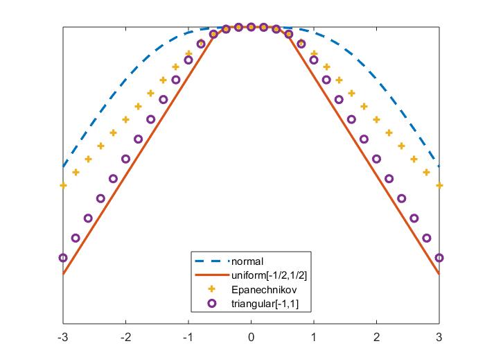
Figure 1: Drift function $\mu\left(r,\varrho;s\right)$ for different kernels (color online)

Since the limiting distribution in (13) depends on unknown components, like $\varrho$ and $\dot{\gamma}_{0}(s)$, it is hard to use this result for further inference. We instead suggest undersmoothing for practical use. More precisely, if we suppose $n^{1-2\epsilon}b_{n}^{2}\rightarrow 0$ as $n\rightarrow\infty$, then the limiting distribution in (13) simplifies to

$$n^{1-2\epsilon}b_{n}\left(\widehat{\gamma}\left(s\right)-\gamma_{0}\left(s\right)\right)\rightarrow_{d}\xi\left(s\right)\arg\max_{r\in\mathbb{R}}\left(W\left(r\right)-\frac{\left|r\right|}{2}\right)$$ (14)

as $n\rightarrow\infty$, which appears the same as in the parametric case in Hansen (2000) except for the scaling factor $n^{1-2\epsilon}b_{n}$. The distribution of $\arg\max_{r\in\mathbb{R}}\left(W\left(r\right)-\left|r\right|/2\right)$ is known (e.g., Bhattacharya and Brockwell (1976) and Bai (1997)), which is also described in Hansen (2000, p.581). The $\xi\left(s\right)$ term determines the scale of the distribution at given $s$ in the way that it increases in the conditional variance $\mathbb{E}[u_{i}^{2}|x_{i},q_{i},s_{i}]$ and decreases in the size of the threshold constant $c_{0}$ and the density of $(q_{i},s_{i})$ near the threshold.

Even when $n^{1-2\epsilon}b_{n}^{2}\rightarrow 0$ as $n\rightarrow\infty$, the asymptotic distribution in (14) still depends on the unknown parameter $\epsilon$ (or equivalently $c_{0}$) in $\xi\left(s\right)$ that is not estimable. Thus, this result cannot be directly used for inference of $\gamma_{0}\left(s\right)$. Alternatively, given any $s\in\mathcal{S}_{0}$, we can consider a pointwise likelihood ratio test statistic for

$$H_{0}:\gamma_{0}\left(s\right)=\gamma_{\ast}\left(s\right)\text{ \ \ against \ \ }H_{1}:\gamma_{0}\left(s\right)\neq\gamma_{\ast}\left(s\right),$$ (15)

which is given as

$$LR_{n}(s)=\mathop{\displaystyle\sum}_{i\in\Lambda_{n}}K\left(\frac{s_{i}-s}{b_{n}}\right)\frac{Q_{n}\left(\gamma_{\ast}\left(s\right),s\right)-Q_{n}\left(\widehat{\gamma}\left(s\right),s\right)}{Q_{n}\left(\widehat{\gamma}\left(s\right),s\right)}\text{.}$$ (16)

The following corollary obtains the limiting null distribution of this test statistic that is free of nuisance parameters. By inverting the likelihood ratio statistic, we can form a pointwise confidence interval for $\gamma_{0}\left(s\right)$.

Corollary 1

Suppose $n^{1-2\epsilon}b_{n}^{2}\rightarrow 0$ as $n\rightarrow\infty$. Under the same condition in Theorem 3, for any fixed $s\in\mathcal{S}_{0}$, the test statistic in (16) satisfies

$$LR_{n}(s)\rightarrow_{d}\xi_{LR}\left(s\right)\max_{r\in\mathbb{R}}\left(2W\left(r\right)-\left|r\right|\right)$$ (17)

as $n\rightarrow\infty$ under the null hypothesis (15), where

$$\xi_{LR}\left(s\right)=\frac{\kappa_{2}c_{0}^{\top}V\left(\gamma_{0}\left(s\right),s\right)c_{0}}{\sigma^{2}(s)c_{0}^{\top}D\left(\gamma_{0}\left(s\right),s\right)c_{0}}$$

with $\sigma^{2}(s)=\mathbb{E}\left[u_{i}^{2}|s_{i}=s\right]$ and $\kappa_{2}=\int K(v)^{2}dv$.

When $\mathbb{E}[u_{i}^{2}|x_{i},q_{i},s_{i}]=\mathbb{E}[u_{i}^{2}|s_{i}]$, which is the case of local conditional homoskedasticity, the scale parameter $\xi_{LR}\left(s\right)$ is simplified as $\kappa_{2}$, and hence the limiting null distribution of $LR_{n}(s)$ becomes free of nuisance parameters and the same for all $s\in\mathcal{S}_{0}$. Though this limiting distribution is still nonstandard, the critical values in this case can be simulated using the same method as Hansen (2000, p.582) with the scale adjusted by $\kappa_{2}$. More precisely, since the distribution function of $\zeta=\max_{r\in\mathbb{R}}\left(2W\left(r\right)-\left|r\right|\right)$ is given as $\mathbb{P}(\zeta\leq z)=(1-\exp(-z/2))^{2}\mathbf{1}\left[z\geq 0\right]$, the distribution function of $\zeta^{\ast}=\kappa_{2}\zeta$ is $\mathbb{P}(\zeta^{\ast}\leq z)=(1-\exp(-z/2\kappa_{2}))^{2}\mathbf{1}\left[z\geq 0\right]$, where $\zeta^{\ast}$ is the limiting random variable of $LR_{n}(s)$ given in (17) under the local conditional homoskedasticity. By inverting it, we can obtain the critical values given a choice of $K(\cdot)$. For instance, the critical values for the Gaussian kernel is reported in Table 1, where $\kappa_{2}=(2\sqrt{\pi})^{-1}\simeq 0.2821$ in this case.

Table 1: Simulated Critical Values of the LR Test (Gaussian Kernel)

$\mathbb{P}(\zeta^{\ast}>cv)$		0.800	0.850	0.900	0.925	0.950	0.975	0.990
$cv$		1.268	1.439	1.675	1.842	2.074	2.469	2.988

Note: $\zeta^{\ast}$ is the limiting distribution of $LR_{n}(s)$ under the local conditional homoskedasticity. The Gaussian kernel is used.

In general, we can estimate $\xi_{LR}\left(s\right)$ by

$$\widehat{\xi}_{LR}\left(s\right)=\frac{\kappa_{2}\widehat{\delta}^{\top}\widehat{V}\left(\widehat{\gamma}\left(s\right),s\right)\widehat{\delta}}{\widehat{\sigma}^{2}(s)\widehat{\delta}^{\top}\widehat{D}\left(\widehat{\gamma}\left(s\right),s\right)\widehat{\delta}},$$

where $\widehat{\delta}$ is from (6) and (7), and $\widehat{\sigma}^{2}(s)$, $\widehat{D}\left(\widehat{\gamma}\left(s\right),s\right)$, and $\widehat{V}\left(\widehat{\gamma}\left(s\right),s\right)$ are the standard Nadaraya-Watson estimators. In particular, we let $\widehat{\sigma}^{2}(s)=\sum_{i\in\Lambda_{n}}\omega_{1i}(s)\widehat{u}_{i}^{2}$ with $\widehat{u}_{i}=y_{i}-x_{i}^{\top}\widehat{\beta}-x_{i}^{\top}\widehat{\delta}\mathbf{1}\left[q_{i}\leq\widehat{\gamma}\left(s_{i}\right)\right]$,

$$\widehat{D}\left(\widehat{\gamma}\left(s\right),s\right)=\mathop{\displaystyle\sum}_{i\in\Lambda_{n}}\omega_{2i}(s)x_{i}x_{i}^{\top}\text{, \ and }\ \widehat{V}\left(\widehat{\gamma}\left(s\right),s\right)=\mathop{\displaystyle\sum}_{i\in\Lambda_{n}}\omega_{2i}(s)x_{i}x_{i}^{\top}\widehat{u}_{i}^{2}\text{,}$$

where

$$\omega_{1i}(s)=\frac{K\left((s_{i}-s)/b_{n}\right)}{\sum_{j\in\Lambda_{n}}K\left((s_{j}-s)/b_{n}\right)}\text{ \ and \ }\omega_{2i}(s)=\frac{\mathbb{K}\left((q_{i}-\widehat{\gamma}\left(s\right))/b_{n}^{\prime},(s_{i}-s)/b_{n}^{\prime\prime}\right)}{\sum_{j\in\Lambda_{n}}\mathbb{K}\left((q_{j}-\widehat{\gamma}\left(s\right))/b_{n}^{\prime},(s_{j}-s)/b_{n}^{\prime\prime}\right)}$$

for some bivariate kernel function $\mathbb{K}(\cdot,\cdot)$ and bandwidth parameters $(b_{n}^{\prime},b_{n}^{\prime\prime})$.

Finally, we show the $\sqrt{n}$-consistency of the semiparametric estimators $\widehat{\beta}$ and $\widehat{\delta}^{\ast}$ in (6) and (7). For this purpose, we first obtain the uniform rate of convergence of $\widehat{\gamma}\left(s\right)$.

Theorem 4

Under Assumptions ID and A,

$$\sup_{s\in\mathcal{S}_{0}}\left|\widehat{\gamma}\left(s\right)-\gamma_{0}\left(s\right)\right|=O_{p}\left(\frac{\log n}{n^{1-2\epsilon}b_{n}}\right)$$

provided that $n^{1-2\epsilon}b_{n}^{2}$ does not diverge.

Apparently, the uniform consistency of $\widehat{\gamma}\left(s\right)$ follows when $\log n/(n^{1-2\epsilon}b_{n})\rightarrow 0$ as $n\rightarrow\infty$. Based on this uniform convergence, the following theorem derives the joint limiting distribution of $\widehat{\beta}$ and $\widehat{\delta}^{\ast}$. We let $\widehat{\theta}^{\ast}=(\widehat{\beta}^{\top},\widehat{\delta}^{\ast\top})^{\top}$ and $\theta_{0}^{\ast}=(\beta_{0}^{\top},\delta_{0}^{\ast\top})^{\top}$.

Theorem 5

Suppose the conditions in Theorem 4 hold. If we let $\pi_{n}>0$ such that $\pi_{n}\rightarrow 0$ and $\{\log n/(n^{1-2\epsilon}b_{n})\}/\pi_{n}\rightarrow 0$ as $n\rightarrow\infty$, we have

$$\sqrt{n}\left(\widehat{\theta}^{\ast}-\theta_{0}^{\ast}\right)\rightarrow_{d}\mathcal{N}\left(0,\Sigma_{X}^{\ast-1}\Omega^{\ast}\Sigma_{X}^{\ast-1}\right)$$ (18)

as $n\rightarrow\infty$, where

$$\Sigma_{X}^{\ast}=\left[\begin{array}[]{cc}\mathbb{E}\left[x_{i}x_{i}^{\top}\mathbf{1}_{i}^{+}\right]&0\\ 0&\mathbb{E}\left[x_{i}x_{i}^{\top}\mathbf{1}_{i}^{-}\right]\end{array}\right]\text{ \ and \ }\Omega^{\ast}=\lim_{n\rightarrow\infty}\frac{1}{n}Var\left[\begin{array}[]{c}\sum_{i\in\Lambda_{n}}x_{i}u_{i}\mathbf{1}_{i}^{+}\\ \sum_{i\in\Lambda_{n}}x_{i}u_{i}\mathbf{1}_{i}^{-}\end{array}\right]$$

with $\mathbf{1}_{i}^{+}=\mathbf{1[}q_{i}>\gamma_{0}(s_{i})]\mathbf{1}[s_{i}\in\mathcal{S}_{0}]$ and $\mathbf{1}_{i}^{-}=\mathbf{1[}q_{i}<\gamma_{0}(s_{i})]\mathbf{1}[s_{i}\in\mathcal{S}_{0}]$.

For the second-step estimator $\widehat{\theta}^{\ast}$, we use (6) and (7), instead of the conventional plug-in estimation, say $\arg\min_{\beta,\delta}\sum_{i\in\Lambda_{n}}(y_{i}-x_{i}^{\top}\beta-x_{i}^{\top}\delta\mathbf{1}[q_{i}\leq\widehat{\gamma}\left(s_{i}\right)])^{2}\mathbf{1}[s_{i}\in\mathcal{S}_{0}]$. The reason is that the first-step nonparametric estimator $\widehat{\gamma}(\cdot)$ may not be asymptotically orthogonal to the second step. Unlike the standard semiparametric literature (e.g., Assumption N(c) in Andrews (1994)), the asymptotic effect of $\widehat{\gamma}\left(s\right)$ to the second-step estimation is not easily derived due to the discontinuity. The new estimation idea above, however, only uses the observations that are little affected by the estimation error in the first step to achieve asymptotic orthogonality. As we verify in Lemma A.17 in the Appendix, this is done by choosing a large enough $\pi_{n}$ in (6) and (7) such that the observations that are included in the second step are outside the uniform convergence bound of $\left|\widehat{\gamma}\left(s\right)-\gamma_{0}\left(s\right)\right|$. Thanks to the threshold regression structure, we can estimate the parameters on each side of the threshold even using these subsamples. Meanwhile, we also want $\pi_{n}\rightarrow 0$ fast enough to include more observations. By doing so, though we lose some efficiency in finite samples, we can derive the asymptotic normality of $\widehat{\theta}=(\widehat{\beta}^{\top},\widehat{\delta}^{\top})^{\top}$ that has zero mean and achieves the same asymptotic variance as if $\gamma_{0}(\cdot)$ was known.

By the delta method, Theorem 5 readily yields the limiting distribution of $\widehat{\theta}=(\widehat{\beta}^{\top},\widehat{\delta}^{\top})^{\top}$ as

$$\sqrt{n}\left(\widehat{\theta}-\theta_{0}\right)\rightarrow_{d}\mathcal{N}\left(0,\Sigma_{X}^{-1}\Omega\Sigma_{X}^{-1}\right)\text{ \ as }n\rightarrow\infty\text{,}$$ (19)

where

$$\Sigma_{X}=\mathbb{E}\left[z_{i}z_{i}^{\top}\mathbf{1}\left[s_{i}\in\mathcal{S}_{0}\right]\right]\text{ \ and \ }\Omega=\lim_{n\rightarrow\infty}\frac{1}{n}Var\left[\sum_{i\in\Lambda_{n}}z_{i}u_{i}\mathbf{1}\left[s_{i}\in\mathcal{S}_{0}\right]\right]$$

with $z_{i}=[x_{i}^{\top},x_{i}^{\top}\mathbf{1}\left[q_{i}\leq\gamma_{0}\left(s_{i}\right)\right]]^{\top}$. The asymptotic variance expressions in (18) and (19) allow for cross-sectional dependence as they have the long-run variance (LRV) forms $\Omega^{\ast}$ and $\Omega$. They can be consistently estimated by the robust estimator developed by Conley and Molinari (2007) using $\widehat{u}_{i}=(y_{i}-x_{i}^{\top}\widehat{\beta}-x_{i}^{\top}\widehat{\delta}\mathbf{1}[q_{i}\leq\widehat{\gamma}\left(s_{i}\right)])\mathbf{1}[s_{i}\in\mathcal{S}_{0}]$. The terms $\Sigma_{X}^{\ast}$ and $\Sigma_{X}$ can be estimated by their sample analogues.

4 Threshold Contour

When we consider sample splitting over a two-dimensional space (i.e., $q_{i}$ and $s_{i}$ respectively correspond to the latitude and longitude on the map), the threshold model (1) can be generalized to estimate a nonparametric contour threshold model:

$$y_{i}=x_{i}^{\top}\beta_{0}+x_{i}^{\top}\delta_{0}\mathbf{1}\left[g_{0}\left(q_{i},s_{i}\right)\leq 0\right]+u_{i}\text{,}$$ (20)

where the unknown function $g_{0}:\mathcal{Q}\times\mathcal{S}\mapsto\mathbb{R}$ determines the threshold contour on a random field that yields sample splitting. An interesting example includes identifying an unknown closed boundary over the map, such as a city boundary, and an area of a disease outbreak or airborne pollution. In social science, it can identify a group boundary or a region in which the agents share common demographic, political, or economic characteristics.

To relate this generalized form to the original threshold model (1), we suppose there exists a known center at $\left(q_{i}^{\ast},s_{i}^{\ast}\right)$ such that $g_{0}\left(q_{i}^{\ast},s_{i}^{\ast}\right)<0$. Without loss of generality, we can normalize $\left(q_{i}^{\ast},s_{i}^{\ast}\right)$ to be $\left(0,0\right)$ and re-center the original location variables $(q_{i},s_{i})$ accordingly. In addition, we define the radius distance $l_{i}$ and angle $a_{i}^{\circ}$ of the $i$th observation relative to the origin as

$$l_{i} = (q_{i}^{2}+s_{i}^{2})^{1/2}\text{,}$$

$$a_{i}^{\circ} = \bar{a}_{i}^{\circ}\mathbf{I}_{i}+\left(180^{\circ}-\bar{a}_{i}^{\circ}\right)\mathbf{II}_{i}+\left(180^{\circ}+\bar{a}_{i}^{\circ}\right)\mathbf{III}_{i}+\left(360^{\circ}-\bar{a}_{i}^{\circ}\right)\mathbf{IV}_{i}\text{,}$$

where $\bar{a}_{i}^{\circ}=\arctan\left(\left|q_{i}/s_{i}\right|\right)$, and each of $(\mathbf{I}_{i},\mathbf{II}_{i},\mathbf{III}_{i},\mathbf{IV}_{i})$ respectively denotes the indicator that the $i$th observation locates in the first, second, third, and forth quadrant.

We suppose that there is only one threshold at any angle and the threshold contour is star-shaped. For each chosen angle $a^{\circ}\in[0^{\circ},360^{\circ})$, we rotate the original coordinate counterclockwise and implement the least squares estimation (5) only using the observations in the first two quadrants after rotation. It will ensure that the threshold mapping after rotation is a well-defined function.

Figure 2: Illustration of rotation (color online)

In particular, the angle relative to the origin is $a_{i}^{\circ}-a^{\circ}$ after rotating the coordinate by $a^{\circ}$ degrees counterclockwise, and the new location (after the rotation) is given as $(q_{i}\left(a^{\circ}\right),s_{i}\left(a^{\circ}\right))$, where

$$\left(\begin{array}[]{c}q_{i}\left(a^{\circ}\right)\\ s_{i}\left(a^{\circ}\right)\end{array}\right)=\left(\begin{array}[]{c}q_{i}\cos\left(a^{\circ}\right)-s_{i}\sin\left(a^{\circ}\right)\\ s_{i}\cos\left(a^{\circ}\right)+q_{i}\sin\left(a^{\circ}\right)\end{array}\right)\text{.}$$

After this rotation, we estimate the following nonparametric threshold model:

$$y_{i}=x_{i}^{\top}\beta_{0}+x_{i}^{\top}\delta_{0}\mathbf{1}\left[q_{i}\left(a^{\circ}\right)\leq\gamma_{a^{\circ}}\left(s_{i}\left(a^{\circ}\right)\right)\right]+u_{i}$$ (21)

using only the observations $i$ satisfying $q_{i}\left(a^{\circ}\right)\geq 0$ and in the neighborhood of $s_{i}\left(a^{\circ}\right)=0$, where $\gamma_{a^{\circ}}\left(\cdot\right)$ is the unknown threshold curve as in the original model (1) on the $a^{\circ}$-degree-rotated coordinate plane. Such reparametrization guarantees that $\gamma_{a^{\circ}}\left(\cdot\right)$ is always positive and it is estimated at the origin. Figure 2 illustrates the idea of such rotation and pointwise estimation over a bounded support so that only the red cross points are included for estimation at different angles. Thus, the estimation and inference procedures developed in the previous sections are directly applicable, though we expect some efficiency loss as we only use the subsample with $q_{i}\left(a^{\circ}\right)\geq 0$ at each $a^{\circ}$.

5 Monte Carlo Experiments

We examine the small sample performance of the semiparametric threshold regression estimator by Monte Carlo simulations. We generate $n$ draws from

$$y_{i}=x_{i}^{\top}\beta_{0}+x_{i}^{\top}\delta_{0}\mathbf{1}\left[q_{i}\leq\gamma_{0}\left(s_{i}\right)\right]+u_{i}\text{,}$$ (22)

where $x_{i}=(1,x_{2i})^{\top}$ and $x_{2i}\in\mathbb{R}$. We let $\beta_{0}=(\beta_{10},\beta_{20})^{\top}=0\iota_{2}$ and consider three different values of $\delta_{0}=(\delta_{10},\delta_{20})^{\top}=\delta\iota_{2}$ with $\delta=1,2,3,4$, where $\iota_{2}=(1,1)^{\top}$. For the threshold function, we let $\gamma_{0}\left(s\right)=\sin(s)/2$. We consider the cross-sectional dependence structure in $\left(x_{2i},q_{i},s_{i},u_{i}\right)^{\top}$ as follows:

$$\left\{\begin{array}[]{l}\left(q_{i},s_{i}\right)^{\top}\sim iid\mathcal{N}\left(0,I_{2}\right)\text{;}\\ x_{2i}|\left(q_{i},s_{i}\right)\sim iid\mathcal{N}\left(0,(1+\rho\left(s_{i}^{2}+q_{i}^{2}\right))^{-1}\right)\text{;}\\ \underline{\mathbf{u}}|\{(x_{i},q_{i},s_{i})\}_{i=1}^{n}\sim\mathcal{N}\left(0,\Sigma\right)\text{,}\end{array}\right.$$ (23)

where $\underline{\mathbf{u}}=(u_{1},\ldots,u_{n})^{\top}$. The $(i,j)$th element of $\Sigma$ is $\Sigma_{ij}=\rho^{\lfloor\ell_{ij}n\rfloor}\mathbf{1}[\ell_{ij}<m/n]$, where $\ell_{ij}=\{\left(s_{i}-s_{j}\right)^{2}+\left(q_{i}-q_{j}\right)^{2}\}^{1/2}$ is the $L^{2}$-distance between the $i$th and $j$th observations. The diagonal elements of $\Sigma$ are normalized as $\Sigma_{ii}=1$. This $m$-dependent setup follows from the Monte Carlo experiment in Conley and Molinari (2007) in the sense that each unit can be cross-sectionally correlated with at most $2m^{2}$ observations. Within the $m$ distance, the dependence decays at a polynomial rate as indicated by $\rho^{\lfloor\ell_{ij}n\rfloor}$. The parameter $\rho$ describes the strength of cross-sectional dependence in the way that a larger $\rho$ leads to stronger dependence relative to the unit standard deviation. In particular, we consider the cases with $\rho=0$ (i.e., i.i.d. observations), $0.5$, and $1$. We consider the sample size $n=100$, $200$, and $500$, and set $\mathcal{S}_{0}$ to include the middle 70% observations of $s_{i}$.

Table 2: Rej. Prob. of the LR Test with i.i.d. Data

		${\small s=0.0}$					${\small s=0.5}$					${\small s=1.0}$
${\small n}$	${\small\delta=}$	1	2	3	4		1	2	3	4		1	2	3	4
100		0.16	0.09	0.06	0.08		0.19	0.10	0.09	0.08		0.25	0.18	0.16	0.12
200		0.09	0.06	0.06	0.07		0.12	0.06	0.04	0.06		0.18	0.09	0.08	0.06
500		0.08	0.05	0.05	0.06		0.08	0.04	0.04	0.05		0.09	0.04	0.04	0.03

Note: Entries are rejection probabilities of the LR test (16) when data are generated from (22) with $\gamma_{0}\left(s\right)=\sin(s)/2$. The dependence structure is given in (23) with $\rho=0$. The significance level is $5\%$ and the results are based on 1000 simulations.

Table 3: Rej. Prob. of the LR Test with Cross-sectionally Correlated Data

		${\small s=0.0}$					${\small s=0.5}$					${\small s=1.0}$
${\small n}$	${\small\delta=}$	1	2	3	4		1	2	3	4		1	2	3	4
100		0.18	0.09	0.07	0.08		0.21	0.11	0.10	0.06		0.28	0.20	0.17	0.13
200		0.12	0.06	0.06	0.06		0.13	0.08	0.06	0.05		0.20	0.37	0.09	0.06
500		0.08	0.04	0.06	0.06		0.06	0.06	0.04	0.05		0.13	0.08	0.05	0.02

Note: Entries are rejection probabilities of the LR test (16) when data are generated from (22) with $\gamma_{0}\left(s\right)=\sin(s)/2$. The dependence structure is given in (23) with $\rho=1$ and $m=10$. The significance level is $5\%$ and the results are based on $1000$ simulations.

First, Tables 2 and 3 report the small sample rejection probabilities of the LR test in (16) for $H_{0}:\gamma_{0}(s)=\sin(s)/2$ against $H_{1}:\gamma_{0}(s)\neq\sin(s)/2$ at the 5% nominal level at three different locations $s=0$, $0.5$, and $1$. In particular, Table 2 examines the case with no cross-sectional dependence ($\rho=0$), while Table 3 examines the case with cross-sectional dependence whose dependence decays slowly with $\rho=1$ and $m=10$. For the bandwidth parameter, we normalize $s_{i}$ and $q_{i}$ to have zero mean and unit standard deviation, and choose $b_{n}=0.5n^{-1/2}$ in the main regression. This choice is for undersmoothing so that $n^{1-2\epsilon}b_{n}^{2}=n^{-2\epsilon}\rightarrow 0$. To estimate $D\left(\gamma_{0}\left(s\right),s\right)$ and $V\left(\gamma_{0}\left(s\right),s\right)$, we use the rule-of-thumb bandwidths from the standard kernel regression satisfying $b_{n}^{\prime}=O(n^{-1/5})$ and $b_{n}^{\prime\prime}=O(n^{-1/6})$. All the results are based on $1000$ simulations. In general, the test for $\gamma_{0}$ performs better as (i) the sample size gets larger; (ii) the coefficient change gets more significant; (iii) the cross-sectional dependence gets weaker; and (iv) the target gets closer to the mid-support of $s$. When $\delta_{0}$ and $n$ are large, the LR test is conservative, which is also found in the classical threshold regression (e.g., Hansen (2000)).

Table 4: Coverage Prob. of the Plug-in Confidence Interval

		$\beta_{20}$					$\beta_{20}+\delta_{20}$					$\delta_{20}$
${\small n}$	${\small\delta=}$	1	2	3	4		1	2	3	4		1	2	3	4
100		0.85	0.87	0.90	0.89		0.82	0.89	0.88	0.88		0.83	0.88	0.89	0.90
200		0.87	0.91	0.91	0.91		0.87	0.90	0.93	0.93		0.86	0.90	0.92	0.94
500		0.89	0.92	0.95	0.94		0.87	0.93	0.93	0.94		0.85	0.92	0.95	0.92

Note: Entries are coverage probabilities of 95% confidence intervals for $\beta_{20}$, $\beta_{20}+\delta_{20},$ and $\delta_{20}$. Data are generated from (22) with $\gamma_{0}\left(s\right)=\sin(s)/2$, where the dependence structure is given in (23) with $\rho=0.5$ and $m=3$. The results are based on 1000 simulations.

Table 5: Coverage Prob. of the Plug-in Confidence Interval (w/ LRV adj.)

		$\beta_{20}$					$\beta_{20}+\delta_{20}$					$\delta_{20}$
${\small n}$	${\small\delta=}$	1	2	3	4		1	2	3	4		1	2	3	4
100		0.94	0.94	0.94	0.94		0.91	0.95	0.95	0.95		0.92	0.94	0.96	0.96
200		0.94	0.95	0.96	0.96		0.93	0.94	0.96	0.96		0.92	0.96	0.97	0.97
500		0.94	0.95	0.98	0.97		0.92	0.96	0.97	0.96		0.91	0.97	0.97	0.96

Note: Entries are coverage probabilities of 95% confidence intervals for $\beta_{20}$, $\beta_{20}$$+\delta_{20},$ and $\delta_{20}$ with a small sample adjustment of the LRV estimator. Data are generated from (22) with $\gamma_{0}\left(s\right)\left.=\right.\sin(s)/2$, where the dependence structure is given in (23) with $\rho=0.5$ and $m=3$. The results are based on 1000 simulations.

Second, Table 4 shows the finite sample coverage properties of the 95% confidence intervals for the parametric components $\beta_{20}$, $\delta_{20}^{\ast}=\beta_{20}+\delta_{20}$, and $\delta_{20}$. The results are based on the same simulation design as above with $\rho=0.5$ and $m=3$. Regarding the tuning parameters, we use the same bandwidth choice $b_{n}=0.5n^{-1/2}$ as before and set the truncation parameter $\pi_{n}=\left(nb_{n}\right)^{-1/2}$. Unreported results suggest that choice of the constant in the bandwidth matters particularly with small samples like $n=100$, but such effect quickly decays as the sample size gets larger. For the estimator of the LRV, we use the spatial lag order of $5$ following Conley and Molinari (2007). Results with other lag choices are similar and hence omitted. The result suggests that the asymptotic normality is better approximated with larger samples and larger change sizes. Table 5 shows the same results with a small sample adjustment of the LRV estimator for $\Omega^{\ast}$ by dividing it by the sample truncation fraction $\sum_{i\in\Lambda_{n}}(\mathbf{1}[q_{i}>\widehat{\gamma}(s_{i})+\pi_{n}]+\mathbf{1}[q_{i}<\widehat{\gamma}(s_{i})-\pi_{n}])\mathbf{1}[s_{i}\in\mathcal{S}_{0}]/\sum_{i\in\Lambda_{n}}\mathbf{1}[s_{i}\in\mathcal{S}_{0}]$. This ratio enlarges the LRV estimator and hence the coverage probabilities, especially when the change size is small. It only affects the finite sample performance as it approaches one in probability as $n\rightarrow\infty$.

6 Applications

6.1 Tipping point and social segregation

The first application is about the tipping point problem in social segregation, which stimulates a vast literature in labor, public, and political economics. Schelling (1971) initially proposes the tipping point model to study the fact that the white population decreases substantially once the minority share exceeds a certain tipping point. Card, Mas, and Rothstein (2008) empirically estimate this model and find strong evidence for such a tipping point phenomenon. In particular, they specify the threshold regression model as

$$y_{i}=\beta_{10}+\delta_{10}\mathbf{1}\left[q_{i}\leq\gamma_{0}\right]+x_{2i}^{\top}\beta_{20}+u_{i}\text{,}$$

where for tract $i$ in a certain city, $q_{i}$ is the minority share in percentage at the beginning of a certain decade, $y_{i}$ is the normalized white population change in percentage within this decade, and $x_{2i}$ is a vector of control variables. They apply the least squares method to estimate the tipping point $\gamma_{0}$. For most cities and for the periods 1970-80, 1980-90, and 1990-2000, they find that white population flows exhibit the tipping-like behavior, with the estimated tipping points ranging approximately from 5% to 20% across cities.

In Section VII of Card, Mas, and Rothstein (2008), they also find that the location of the tipping point substantially depends on white residents’ attitudes toward the minority. Specifically, they first construct a city-level index that measures white attitudes and regress the estimated tipping point from each city on this index. The regression coefficient is significantly different from zero, suggesting that the tipping point is heterogeneous across cities.

We go one step further by considering a more flexible model in the tract level given as

$$y_{i}=\beta_{10}+\delta_{10}\mathbf{1}\left[q_{i}\leq\gamma_{0}(s_{i})\right]+x_{2i}^{\top}\beta_{20}+u_{i}\text{,}$$

where $\gamma_{0}(\cdot)$ denotes an unknown tipping point function and $s_{i}$ denotes the attitude index. The nonparametric function $\gamma_{0}(\cdot)$ here allows for heterogeneous tipping points across tracts depending on the level of the attitude index $s_{i}$ in tract $i$. Unfortunately, the attitude index by Card, Mas, and Rothstein (2008) is only available at the aggregated city-level, and hence we cannot use it to analyze the census tract-level observations. For this reason, we instead use the tract-level unemployment rate as $s_{i}$ to illustrate the nonparametric threshold function, which is readily available in the original dataset. Such a compromise is far from being perfect but can be partially justified since race discrimination has been widely documented to be correlated with employment (e.g., Darity and Mason (1998)).

Figure 3: Estimate of the tipping point as a function of the unemployment rate

Panel A: Estimated tipping point function in Chicago 1980-90

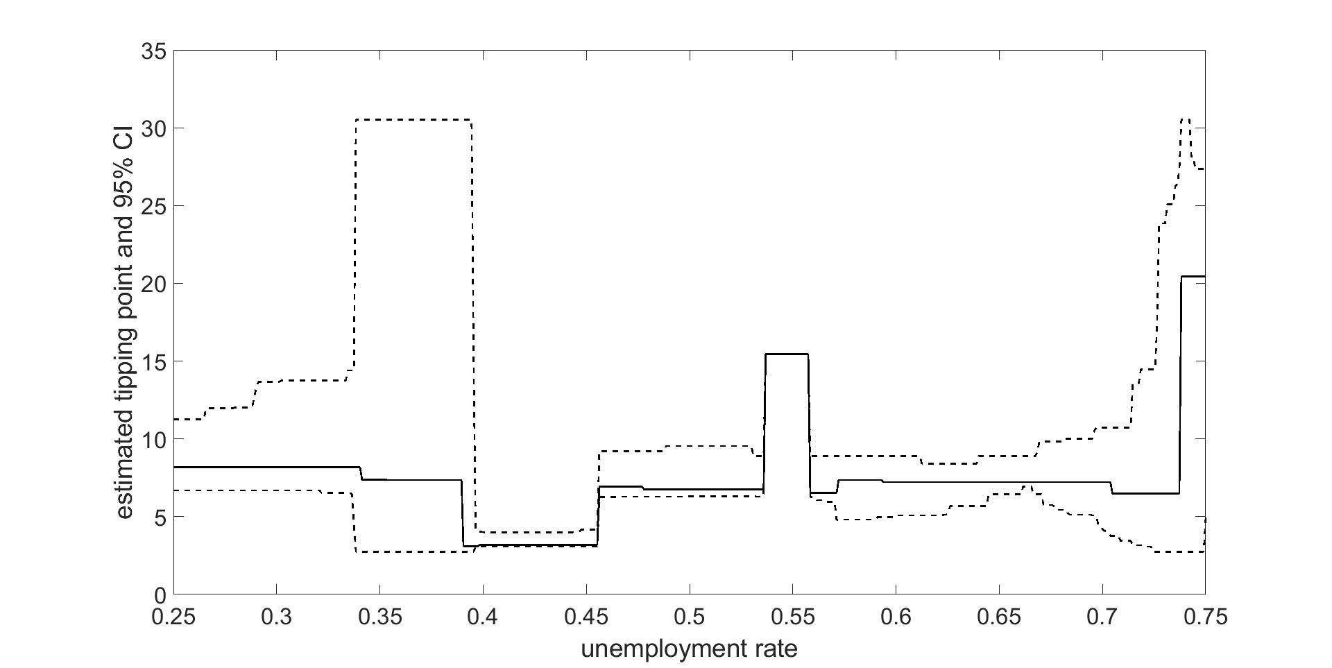
Panel B: Estimated tipping point function in Los Angeles 1980-90

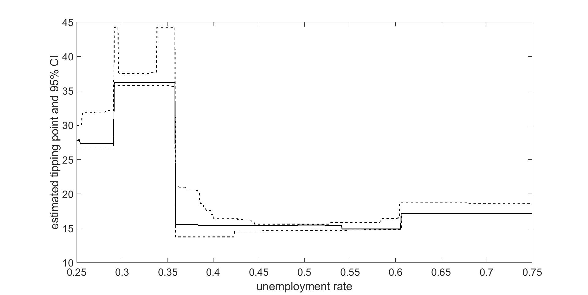
Panel C: Estimated tipping point function in New York City 1980-90

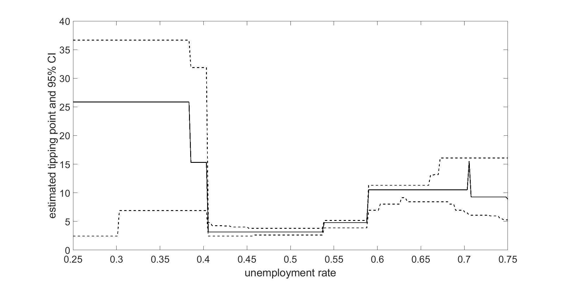
Note: The figure depicts the point estimate of the tipping points as a function of the unemployment rate, using the data in Chicago, Los Angeles, and New York City in 1980-1990. The vertical axis is the estimated tipping point in percentage, and the horizontal axis is the tract-level unemployment normalized into quantile level. Data are available from Card, Mas, and Rothstein (2008).

We use the data provided by Card, Mas, and Rothstein (2008) and estimate the tipping point function $\gamma_{0}(\cdot)$ over census tracts by the method introduced in Section 2. As in their work, we drop the tracts where the minority shares are above 60 percentage points and use five control variables as $x_{2i}$, including the logarithm of mean family income, the fractions of single-unit, vacant, and renter-occupied housing units, and the fraction of workers who use public transport to travel to work. The bandwidth is set as $b_{n}=cn^{-1/2}$ for some $c>0$, so that it satisfies the technical conditions in the previous sections, where the constant $c$ is chosen by the leave-one-out cross validation. In particular, we first construct the leave-one-out estimate, $\widehat{\gamma}_{-i}\left(s_{i}\right)$, of $\gamma_{0}\left(s_{i}\right)$ as in (4) without using the $i$th observation. Then, leaving the $i$th observation out, we construct $\widehat{\beta}_{-i}$ and $\widehat{\delta}_{-i}$ as in (6) and (7) with $\pi_{n}=\left(nb_{n}\right)^{-1/2}$ using the bandwidth $b_{n}$ chosen in the previous step. We choose the bandwidth that minimizes $\sum_{i\in\Lambda_{n}}(y_{i}-\widehat{\beta}_{1,-i}-\widehat{\delta}_{1,-i}\mathbf{1}\left[q_{i}\leq\widehat{\gamma}_{-i}(s_{i})\right]-x_{2i}^{\top}\widehat{\beta}_{2,-i})^{2}\mathbf{1}\left[s_{i}\in\mathcal{S}_{0}\right]$, where $\mathcal{S}_{0}$ again includes the middle 70% quantiles of $s_{i}$.

Figure 3 depicts the estimated tipping points and the 95% pointwise confidence intervals by inverting the likelihood ratio test statistic (16) in the years 1980-90 in Chicago, Los Angeles, and New York City, whose sample sizes are relatively large. For each city, the constant $c$ of the bandwidth $b_{n}=cn^{-1/2}$ chosen by the aforementioned cross validation is $3.20$, $4.87$, and $3.42$, respectively. We make the following comments. First, the estimates of the tipping points vary substantially in the unemployment rate within all three cities. Therefore, the standard constant tipping point model is insufficient to characterize the segregation fully. Second, the tipping points as functions of the unemployment rate do not exhibit the same pattern across cities, reinforcing the heterogeneous tipping points in the city-level as found in Card, Mas, and Rothstein (2008). Finally, the estimated tipping point $\widehat{\gamma}\left(s\right)$ as a function of $s$ can be discontinuous, which does not contrast with Assumption A-(vi), that is, the true function $\gamma_{0}\left(\cdot\right)$ is smooth. The discontinuity comes from the fact that $\widehat{\gamma}\left(s\right)$ is obtained by grid search and can only take values among the discrete points $\{q_{1},...,q_{n}\}$ in finite samples.

6.2 Metropolitan area determination

The second application is about determining the boundary of a metropolitan area, which is a fundamental question in urban economics. Recently, researchers propose to use nighttime light intensity obtained by satellite imagery to define metropolitan areas. The intuition is straightforward: metropolitan areas are bright at night while rural areas are dark.

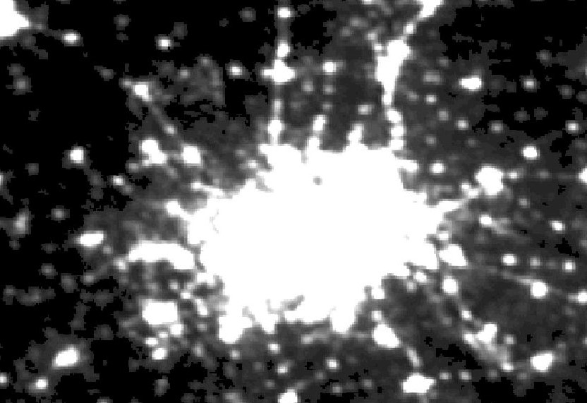
Figure 4: Nighttime light intensity in Dallas, Texas, in 2010

Note: The figure depicts the intensity of the stable nighttime light in Dallas, TX 2010. Data are available from https://www.ncei.noaa.gov/. 

Specifically, the National Oceanic and Atmospheric Administration (NOAA) collects satellite imagery of nighttime lights at approximately 1-kilometer resolution since 1992. NOAA further constructs several indices measuring the annual light intensity. Following the literature (e.g., Dingel, Miscio, and Davis (2019)), we choose the “average visible, stable lights” index that ranges from 0 (dark) to 63 (bright). For illustration, we focus on Dallas, Texas and use the data from the years 1995, 2000, 2005, and 2010. In each year, the data are recorded as a 240$\times$360 grid that covers the latitudes from 32^∘N to 34^∘N and the longitudes from 98.5^∘W to 95.5^∘W. The total sample size is 240$\times$360=86400 each year. These data are available at NOAA’s website and also provided on the authors’ website. Figure 4 depicts the intensity of the stable nighttime light of the Dallas area in 2010 as an example.

Let $y_{i}$ be the level of nighttime light intensity and $\left(q_{i},s_{i}\right)$ be the latitude and longitude of the $i$th pixel, which is normalized into the equally-spaced grids on $[0,1]^{2}$. To define the metropolitan area, existing literature in urban economics first chooses an ad hoc intensity threshold, say 95% quantile of $y_{i}$, and categorizes the $i$th pixel as a part of the metropolitan area if $y_{i}$ is larger than the threshold. See Dingel, Miscio, and Davis (2019), Vogel, Goldblatt, Hanson, and Khandelwal (2019), and references therein. In particular, on p.3 in Dingel, Miscio, and Davis (2019), they note that “[…] the choice of the light-intensity threshold, which governs the definitions of the resulting metropolitan areas, is not pinned down by economic theory or prior empirical research.” Our new approach can provide a data-driven guidance of choosing the intensity threshold from the econometric perspective.

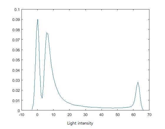
Figure 5: Kernel density estimate of nighttime light intensity, Dallas 2010

Note: The figure depicts the kernel density estimate of the strength of the stable nighttime light in Dallas, TX 2010. Data are available from https://www.ncei.noaa.gov/. 

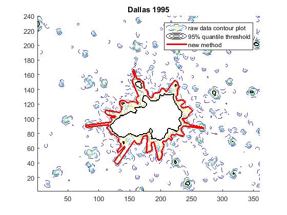
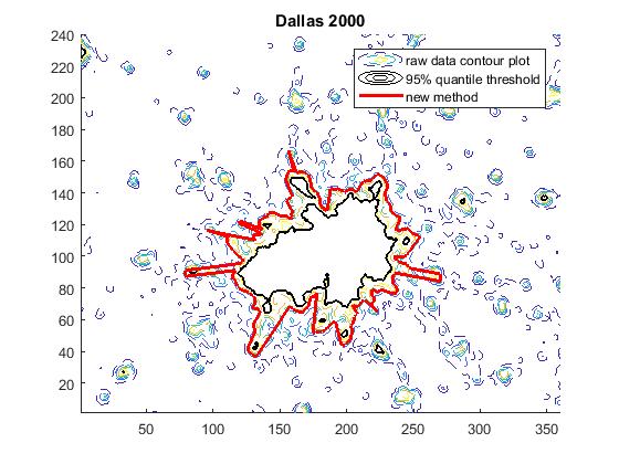
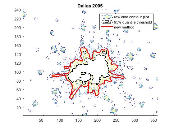
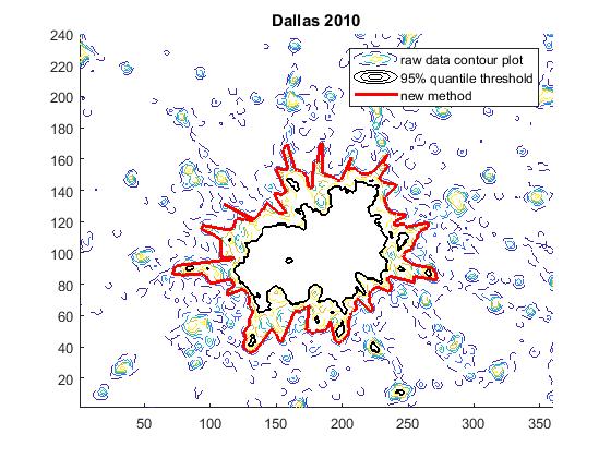
Figure 6: Metropolitan area determination in Dallas (color online)

Note: The figure depicts the city boundary determined by either the new method or by taking the 0.95 quantile of nighttime light strength as the threshold, using the satellite imagery data for Dallas, TX in the years 1995, 2000, 2005, and 2010. Data are available from https://www.ncei.noaa.gov/. 

To this end, we first examine whether the light intensity data exhibits a clear threshold pattern. We plot the kernel density estimates of $y_{i}$ in the year 2010 in Figure 5. The bandwidth is the standard rule-of-thumb one. The estimated density exhibits three peaks at around the intensity levels 0, 8, and 63. They respectively correspond to the rural area, small towns, and the central metropolitan area. It shows that the threshold model is appropriate in characterizing such a mean-shift pattern.

Now we implement the rotation and estimation method described in Section 4. In particular, we pick the center point in the bright middle area as the Dallas metropolitan center, which corresponds to the pixel point in the 181st column from the left and the 100th row from the bottom. Then for each $a^{\circ}$ over the 500 equally-spaced grid on $[0^{\circ},360^{\circ}]$, we rotate the data by $a^{\circ}$ degrees counterclockwise and estimate the model (21) with $x_{i}=1$. The bandwidth is chosen as $cn^{-1/2}$ with $c=1$. Other choices of $c$ lead to almost identical results, given the large sample size. Figure 6 presents the estimated metropolitan areas using our nonparametric approach (red) and the area determined by the ad hoc threshold of the 95% quantile of $y_{i}$ (black) in the years 1995, 2000, 2005, and 2010. It clearly shows the expansion of the Dallas metropolitan area over the 15 years of the sample period.

Several interesting findings are summarized as follows. First, the estimated boundary is highly nonlinear as a function of the angle. Therefore, any parametric threshold model could lead to a substantially misleading result. Second, our estimated area is larger than that determined by the ad hoc threshold, by 80.31%, 81.56%, 106.46%, and 102.09% in the years 1995, 2000, 2005, and 2010, respectively. In particular, our nonparametric estimates tend to include some suburban areas that exhibit strong light intensity and that are geographically close to the city center. For example, the very left stretch-out area in the estimated boundary corresponds to Fort Worth, which is 30 miles from downtown Dallas. Residents can easily commute by train or driving on the interstate highway 30. It is then reasonable to include Fort Worth as a part of the metropolitan Dallas area for economic analysis. Third, given the large sample size, the 95% confidence intervals of the boundary are too narrow to be distinguished from the estimates and therefore omitted from the figure. Such narrow intervals apparently exclude the boundary determined by the ad hoc method. Finally, the estimated value of $\beta_{0}+\delta_{0}$ is approximately $53$ in these sample periods, which corresponds to the 89% quantile of $y_{i}$ in the sample. This suggests that a more proper choice of the level of light intensity threshold is the 89% quantile of $y_{i}$, instead of the 95% quantile, if one needs to choose the light-intensity threshold to determine the Dallas metropolitan area.

7 Concluding Remarks

This paper proposes a novel approach to conduct sample splitting. In particular, we develop a nonparametric threshold regression model where two variables can jointly determine the unknown threshold boundary. Our approach can be easily generalized so that the sample splitting depends on more numbers of variables, though such an extension is subject to the curse of dimensionality, as usually observed in the kernel regression literature. The main interest is in identifying the threshold function that determines how to split the sample. Thus our model should be distinguished from the smoothed threshold regression model or the random coefficient regression model. It instead could be seen as an unsupervised learning tool for clustering.

This new approach is empirically relevant in broad areas studying sample splitting (e.g., segregation and group-formation) and heterogeneous effects over different subsamples. We illustrate some of them with the tipping point problem in social segregation and metropolitan area determination using satellite imagery datasets. Though we omit in this paper, we also estimate the economic border between Brooklyn and Queens boroughs in New York City using housing prices. The estimated border is substantially different from the existing administrative border, which was determined in 1931 and cannot reflect the dramatic city development. Interestingly, the estimated border coincides with the Jackson Robinson Parkway and the Long Island Railroad. This finding provides new evidence that local transportation corridors could increase community segregation (cf. Ananat (2011) and Heilmann (2018)).

We list some related works, which could motivate potential theoretical extensions. First, while we focus on the local constant estimation in this paper, one could consider the local linear estimation using the threshold indicator $\mathbf{1}\left[q_{i}\leq\gamma_{1}+\gamma_{2}(s_{i}-s)\right]$ in (3). Although grid search is very difficult in determining the two threshold parameters ($\gamma_{1}$ and $\gamma_{2}$), we could use the MCMC algorithm developed by Yu and Fan (2020) and the mixed integer optimization (MIO) algorithms developed by Lee, Liao, Seo, and Shin (2020). Besides the computational challenge, however, the asymptotic derivation is more involved since we need to consider higher-order expansions of the objective function. Second, while our nonparametric setup is on the threshold function $\gamma_{0}(\cdot)$, some recent literature studies the nonparametric regression model with a parametric threshold, such as $y_{i}=m_{1}(x_{i})+m_{2}(x_{i})\mathbf{1}[q_{i}\leq\gamma_{0}]+u_{i}$, where $m_{1}\left(\cdot\right)$ and $m_{2}\left(\cdot\right)$ are different nonparametric functions. See, for example, Henderson, Parmeter, and Su (2017), Chiou, Chen, and Chen (2018), Yu and Phillips (2018), Yu, Liao, and Phillips (2019), and Delgado and Hidalgo (2000).

Appendix A Appendix

Throughout the proof, we denote $K_{i}\left(s\right)=K\left((s_{i}-s)/b_{n}\right)$ and $\mathbf{1}_{i}\left(\gamma\right)=\mathbf{1}\left[q_{i}\leq\gamma\right]$. We let $C$ and its variants such as $C_{1}$ and $C_{1}^{\prime}$ stand for generic positive finite constants that may vary across lines. We also let $a_{n}=n^{1-2\epsilon}b_{n}$. All the additional lemmas in the proof assume the conditions in Assumptions ID and A hold. Omitted proofs for some lemmas are all collected in the supplementary material.

A.1 Proof of Theorem 1 (Identification)

Proof of Theorem 1

First, for any $\gamma(s)\in\Gamma$ with given $s\in\mathcal{S}$, we define an $L_{2}$-loss as

$$R(\beta,\delta,\gamma;s) = \mathbb{E}\left[\left.\left(y_{i}-x_{i}^{\top}\beta-x_{i}^{\top}\delta\mathbf{1}_{i}\left(\gamma(s_{i})\right)\right)^{2}\right|s_{i}=s\right]$$

$$-\mathbb{E}\left[\left.\left(y_{i}-x_{i}^{\top}\beta_{0}-x_{i}^{\top}\delta_{0}\mathbf{1}_{i}\left(\gamma_{0}(s_{i})\right)\right)^{2}\right|s_{i}=s\right]\text{.}$$

For any $\gamma\in\Gamma\equiv[\underline{\gamma},\overline{\gamma}]$, we have $\mathbb{E}[R(\beta,\delta,\gamma;s_{i})]\geq 0$ from Assumption ID-(i). Since

$$R(\beta,\delta,\gamma;s)=\left\{\begin{array}[]{ll}\mathbb{E}\left[\left.\left(x_{i}^{\top}((\beta+\delta)-\mathbf{(}\beta_{0}+\delta_{0}\mathbf{)}\right)^{2}\right|s_{i}=s\right]&\text{for }q_{i}\leq\min\{\gamma(s),\gamma_{0}(s)\}\text{;}\\ \mathbb{E}\left[\left.\left(x_{i}^{\top}\left(\beta-\beta_{0}\right)\right)^{2}\right|s_{i}=s\right]&\text{for }q_{i}>\max\{\gamma(s),\gamma_{0}(s)\}\text{,}\end{array}\right.$$

we have

$$\mathbb{E}\left[R(\beta,\delta,\gamma;s_{i})\right] \geq \left\|(\beta-\beta_{0})+\mathbf{(}\delta-\delta_{0}\mathbf{)}\right\|^{2}\mathbb{E}\left[||x_{i}x_{i}^{\top}||\mathbf{1}\left[q_{i}\leq\underline{\gamma}\right]\right]$$

$$+\left\|\beta-\beta_{0}\right\|^{2}\mathbb{E}\left[||x_{i}x_{i}^{\top}||\mathbf{1}\left[q_{i}>\overline{\gamma}\right]\right]$$

$$> 0$$

when $(\beta^{\top},\delta^{\top})^{\top}\neq(\beta_{0}^{\top},\delta_{0}^{\top})^{\top}$ from Assumption ID-(ii). Therefore, we have $\mathbb{E}\left[R(\beta,\delta,\gamma;s_{i})\right]=0$ only when $(\beta^{\top},\delta^{\top})^{\top}=(\beta_{0}^{\top},\delta_{0}^{\top})^{\top}$, which gives that $(\beta_{0}^{\top},\delta_{0}^{\top})^{\top}$ are identified as the unique minimizer of $\mathbb{E}[\left(y_{i}-x_{i}^{\top}\beta-x_{i}^{\top}\delta\mathbf{1}_{i}\left(\gamma\right)\right)^{2}]$ for any $\gamma\in\Gamma$.

Second, note that we have $R(\beta_{0},\delta_{0},\gamma;s)\geq 0$ for any $\gamma(s)\in\Gamma$ with given $s\in\mathcal{S}$ from Assumption ID-(i). For any $\gamma(s)\neq\gamma_{0}(s)$ at $s_{i}=s$ and $(\beta^{\top},\delta^{\top})^{\top}=(\beta_{0}^{\top},\delta_{0}^{\top})^{\top}$, however, we have

$$R(\beta_{0},\delta_{0},\gamma;s)$$

$$= \delta_{0}^{\top}\mathbb{E}\left[\left.x_{i}x_{i}^{\top}\left(\mathbf{1}_{i}\left(\gamma(s_{i})\right)-\mathbf{1}_{i}\left(\gamma_{0}(s_{i})\right)\right)^{2}\right|s_{i}=s\right]\delta_{0}$$

$$= \delta_{0}^{\top}\mathbb{E}\left[\left.x_{i}x_{i}^{\top}\mathbf{1}\left[\min\{\gamma(s_{i}),\gamma_{0}(s_{i})\}<q_{i}\leq\max\{\gamma(s_{i}),\gamma_{0}(s_{i})\}\right]\right|s_{i}=s\right]\delta_{0}$$

$$= \int_{\min\{\gamma(s),\gamma_{0}(s)\}}^{\max\{\gamma(s),\gamma_{0}(s)\}}\delta_{0}^{\top}\mathbb{E}\left[\left.x_{i}x_{i}^{\top}\right|q_{i}=q,s_{i}=s\right]\delta_{0}f(q|s)dq$$

$$\geq C(s)\mathbb{P}\left(\left.\min\{\gamma(s_{i}),\gamma_{0}(s_{i})\}<q_{i}\leq\max\{\gamma(s_{i}),\gamma_{0}(s_{i})\}\right|s_{i}=s\right)$$

$$> 0$$

from Assumptions ID-(i), (iii), and (iv), where $C(s)=\inf_{q\in\mathcal{Q}}\delta_{0}^{\top}\mathbb{E}[x_{i}x_{i}^{\top}|q_{i}=q,s_{i}=s]\delta_{0}>0$. Note that the last probability is strictly positive because we assume $f(q|s)>0$ for any $(q,s)\in\Gamma\times\mathcal{S}$ and $\gamma_{0}(s)$ is not located on the boundary of $\mathcal{Q}$ as $\varepsilon(s)<\mathbb{P}(q_{i}\leq\gamma_{0}(s_{i})|s_{i}=s)<1-\varepsilon(s)$ for some $\varepsilon(s)>0$. Therefore, $R(\beta_{0},\delta_{0},\gamma;s)=0$ only when $\gamma(s)=\gamma_{0}(s)$ since $R(\beta_{0},\delta_{0},\gamma;s)$ is continuous at $\gamma=\gamma_{0}(s)$ and $\gamma$ is in a compact support from Assumptions ID-(ii) and (iv). It gives that $\gamma_{0}(s)$ is identified as the unique minimizer of $\mathbb{E}[\left(y_{i}-x_{i}^{\top}\beta_{0}-x_{i}^{\top}\delta_{0}\mathbf{1}_{i}\left(\gamma(s_{i})\right)\right)^{2}|s_{i}=s]$ for each $s\in\mathcal{S}$. $\blacksquare$

A.2 Proof of Theorem 2 (Pointwise Convergence)

We first present a covariance inequality for strong mixing random field. Suppose $\Lambda_{1}$ and $\Lambda_{2}$ are finite subsets in $\Lambda_{n}$ with $\left|\Lambda_{1}\right|=k_{x},\left|\Lambda_{2}\right|=l_{x}$, and let $X_{1}$ and $X_{2}$ be random variables respectively measurable with respect to the $\sigma$-algebra’s generated by $\Lambda_{1}$ and $\Lambda_{2}$. If $\mathbb{E}\left[\left|X_{1}\right|^{p_{x}}\right]<\infty$ and $\mathbb{E}\left[\left|X_{2}\right|^{q_{x}}\right]<\infty$ with $1/p_{x}+1/q_{x}+1/r_{x}=1$ for some constants $p_{x},q_{x}>1$ and $r_{x}>0$, then

$$\left|Cov\left[X_{1},X_{2}\right]\right|<8\alpha_{k_{x},l_{x}}(\lambda(\Lambda_{1},\Lambda_{2}))^{1/r_{x}}\mathbb{E}\left[\left|X_{1}\right|^{p_{x}}\right]^{1/p_{x}}\mathbb{E}\left[\left|X_{2}\right|^{q_{x}}\right]^{1/q_{x}}$$ (A.1)

under Assumptions A-(i) and A-(iii). This covariance inequality is presented as Lemma 1 in the working paper version of Jenish and Prucha (2009). The proof is also available in Hall and Heyde (1980), p.277.

For a given $s\in\mathcal{S}_{0}$, we define

$$M_{n}(\gamma;s) = \frac{1}{nb_{n}}\mathop{\displaystyle\sum}_{i\in\Lambda_{n}}x_{i}x_{i}^{\top}\mathbf{1}_{i}(\gamma)K_{i}(s)$$

$$J_{n}(\gamma;s) = \frac{1}{\sqrt{nb_{n}}}\mathop{\displaystyle\sum}_{i\in\Lambda_{n}}x_{i}u_{i}\mathbf{1}_{i}(\gamma)K_{i}(s).$$

The following four lemmas give the asymptotic behavior of $M_{n}(\gamma;s)$ and $J_{n}(\gamma;s)$.

Lemma A.1 (Maximal inequality)

For any given $s\in\mathcal{S}_{0}$, any $\eta,\varpi>0$, and any $\gamma_{1}\in\Gamma$, there exists a constant $C^{\ast}$ such that

$$\mathbb{P}\left(\sup_{\gamma\in[\gamma_{1},\gamma_{1}+\varpi]}\left\|J_{n}\left(\gamma;s\right)-J_{n}\left(\gamma_{1};s\right)\right\|>\eta\right)\leq\frac{C^{\ast}\varpi^{2}}{\eta^{4}}$$

if $n$ is sufficiently large.

Proof of Lemma A.1

For expositional simplicity, we only present the case of scalar $x_{i}$. Let $\varpi$ be such that $\varpi\geq(nb_{n})^{-1}$ and $\overline{g}$ be an integer satisfying $nb_{n}\varpi/2\leq\overline{g}\leq nb_{n}\varpi$, which always exists since $nb_{n}\varpi\geq 1$. Consider a fine enough grid over $[\gamma_{1},\gamma_{1}+\varpi]$ such that $\gamma_{g}=\gamma_{1}+(g-1)\varpi/\overline{g}$ for $g=1,\ldots,\overline{g}+1$, where $\max_{1\leq g\leq\overline{g}}\left(\gamma_{g}-\gamma_{g-1}\right)\leq\varpi/\overline{g}$. We define $h_{ig}(s)=x_{i}u_{i}K_{i}\left(s\right)\mathbf{1}\left[\gamma_{g}<q_{i}\leq\gamma_{g+1}\right]$ and $H_{ng}(s)=(nb_{n})^{-1}\sum_{i\in\Lambda_{n}}|h_{ig}(s)|$ for $1\leq g\leq\overline{g}$. Then for any $\gamma\in\left[\gamma_{g},\gamma_{g+1}\right]$,

$$\left|J_{n}\left(\gamma;s\right)-J_{n}\left(\gamma_{g};s\right)\right| \leq \sqrt{nb_{n}}H_{ng}(s)$$

$$\leq \sqrt{nb_{n}}\left|H_{ng}(s)-\mathbb{E}\left[H_{ng}(s)\right]\right|+\sqrt{nb_{n}}\mathbb{E}\left[H_{ng}(s)\right]$$

and hence

$$\sup_{\gamma\in[\gamma_{1},\gamma_{1}+\varpi]}\left|J_{n}\left(\gamma;s\right)-J_{n}\left(\gamma_{1};s\right)\right|$$

$$\leq \max_{2\leq g\leq\overline{g}+1}\left|J_{n}\left(\gamma_{g};s\right)-J_{n}\left(\gamma_{1};s\right)\right|$$

$$+\max_{1\leq g\leq\overline{g}}\sqrt{nb_{n}}\left|H_{ng}(s)-\mathbb{E}\left[H_{ng}(s)\right]\right|+\max_{1\leq g\leq\overline{g}}\sqrt{nb_{n}}\mathbb{E}\left[H_{ng}(s)\right]$$

$$\equiv \Psi_{1}(s)+\Psi_{2}(s)+\Psi_{3}(s)\text{.}$$

We let $h_{i}(s)=x_{i}u_{i}K_{i}\left(s\right)\mathbf{1}\left[\gamma_{g}<q_{i}\leq\gamma_{k}\right]$ for any given $1\leq g<k\leq\overline{g}$ and for fixed $s$. First, for $\Psi_{1}(s)$, we have

$$\mathbb{E}\left[\left|J_{n}\left(\gamma_{g};s\right)-J_{n}\left(\gamma_{k};s\right)\right|^{4}\right]$$

$$= \frac{1}{n^{2}b_{n}^{2}}\mathop{\displaystyle\sum}_{i\in\Lambda_{n}}\mathbb{E}\left[h_{i}^{4}(s)\right]+\frac{1}{n^{2}b_{n}^{2}}\mathop{\displaystyle\sum}_{\begin{subarray}{c}i,j\in\Lambda_{n}\\ i\neq j\end{subarray}}\mathbb{E}\left[h_{i}^{2}(s)h_{j}^{2}(s)\right]+\frac{1}{n^{2}b_{n}^{2}}\mathop{\displaystyle\sum}_{\begin{subarray}{c}i,j\in\Lambda_{n}\\ i\neq j\end{subarray}}\mathbb{E}\left[h_{i}^{3}(s)h_{j}(s)\right]$$

$$+\frac{1}{n^{2}b_{n}^{2}}\mathop{\displaystyle\sum}_{\begin{subarray}{c}i,j,k,l\in\Lambda_{n}\\ i\neq j\neq k\neq l\end{subarray}}\mathbb{E}\left[h_{i}(s)h_{j}(s)h_{k}(s)h_{l}(s)\right]+\frac{1}{n^{2}b_{n}^{2}}\mathop{\displaystyle\sum}_{\begin{subarray}{c}i,j,k\in\Lambda_{n}\\ i\neq j\neq k\end{subarray}}\mathbb{E}\left[h_{i}^{2}(s)h_{j}(s)h_{k}(s)\right]$$

$$\equiv \Psi_{11}(s)+\Psi_{12}(s)+\Psi_{13}(s)+\Psi_{14}(s)+\Psi_{15}(s)\text{,}$$

where each term’s bound is obtained as follows.

For $\Psi_{11}(s)$, since $\mathbb{E}[|x_{i}u_{i}|^{4}|q_{i},s_{i}]\mathbf{1}[\gamma_{g}<q_{i}\leq\gamma_{k}]<C_{1}<\infty$ from Assumption A-(v), we have

$$\frac{1}{b_{n}}\mathbb{E}\left[h_{i}^{4}(s)\right] = \frac{1}{b_{n}}\iint\mathbb{E}\left[|x_{i}u_{i}|^{4}|q,v\right]1\left[\gamma_{g}<q\leq\gamma_{k}\right]K^{4}\left(\frac{v-s}{b_{n}}\right)f\left(q,v\right)dqdv$$

$$\leq \frac{C_{1}}{b_{n}}\iint K^{4}\left(\frac{v-s}{b_{n}}\right)f\left(q,v\right)dqdv$$

$$= C_{1}\iint K^{4}\left(t\right)f\left(q,s+b_{n}t\right)dqdt$$

$$= C_{1}(s)+O\left(b_{n}^{2}\right)$$

for some $C_{1}(s)<\infty$ for a given $s$ from Assumption A-(x), where we apply the change of variables $t=(v-s)/b_{n}$. Hence, $\Psi_{11}(s)=O(n^{-1}b_{n}^{-1})=o(1)$. For $\Psi_{12}(s)$, by the covariance inequality (A.1) with $p_{x}=2+\varphi$, $q_{x}=2+\varphi$, $r_{x}=(2+\varphi)/\varphi$, and $k_{x}=l_{x}=1$,

$$\frac{1}{n^{2}b_{n}^{2}}\mathop{\displaystyle\sum}_{\begin{subarray}{c}i,j\in\Lambda_{n}\\ i\neq j\end{subarray}}\left|Cov\left[h_{i}^{2}(s),h_{j}^{2}(s)\right]\right|$$

$$\leq \frac{C_{2}}{n^{2}b_{n}^{2}}\mathop{\displaystyle\sum}_{\begin{subarray}{c}i,j\in\Lambda_{n}\\ i\neq j\end{subarray}}\alpha_{1,1}(\lambda(i,j))^{\varphi/(2+\varphi)}\mathbb{E}\left[\left|h_{i}^{2}(s)\right|^{2+\varphi}\right]^{2/\left(2+\varphi\right)}$$

$$\leq \frac{C_{2}}{n^{2}b_{n}^{2}}\mathbb{E}\left[\left|h_{i}^{2}(s)\right|^{2+\varphi}\right]^{2/\left(2+\varphi\right)}\mathop{\displaystyle\sum}_{i\in\Lambda_{n}}\mathop{\displaystyle\sum}_{m=1}^{n-1}\mathop{\displaystyle\sum}_{\begin{subarray}{c}j\in\Lambda_{n}\\ \lambda(i,j)\in[m,m+1)\end{subarray}}\alpha_{1,1}\left(m\right)^{\varphi/(2+\varphi)}$$

$$\leq \frac{C_{2}^{\prime}}{n^{2}b_{n}^{2}}\mathbb{E}\left[\left|h_{i}^{2}(s)\right|^{2+\varphi}\right]^{2/\left(2+\varphi\right)}\mathop{\displaystyle\sum}_{i\in\Lambda_{n}}\mathop{\displaystyle\sum}_{m=1}^{\infty}m\alpha_{1,1}\left(m\right)^{\varphi/(2+\varphi)}$$

$$\leq \frac{C_{2}^{\prime\prime}}{n^{2}b_{n}^{(2+2\varphi)/(2+\varphi)}}\left(\frac{1}{b_{n}}\mathbb{E}\left[\left|h_{i}^{2}(s)\right|^{2+\varphi}\right]\right)^{2/\left(2+\varphi\right)}n\mathop{\displaystyle\sum}_{m=1}^{\infty}m\exp\left(-m\varphi/(2+\varphi)\right)$$

for some $\varphi>0$ and $C_{2},C_{2}^{\prime},C_{2}^{\prime\prime}<\infty$, where $b_{n}^{-1}\mathbb{E}[\left|h_{i}^{2}(s)\right|^{2+\varphi}]<\infty$ as in (A.2). Note that $\alpha_{1,1}(\lambda(i,j))\leq\alpha_{1,1}(m)$ for $\lambda(i,j)\in[m,m+1)$ and $|\{j\in\Lambda_{n}:\lambda(i,j)\in[m,m+1)\}|=O(m)$ for any given $i\in\Lambda_{n}$ as in Lemma A.1.(iii) of Jenish and Prucha (2009). Furthermore, by Assumptions A-(vii) and (x),

$$\frac{1}{b_{n}}\mathbb{E}\left[h_{i}^{2}(s)\right] = \iint V\left(q,t\right)1\left[\gamma_{g}<q\leq\gamma_{k}\right]K^{2}\left(t\right)f\left(q,s+tb_{n}\right)dqdt$$

$$= \iint V\left(q,t\right)1\left[\gamma_{g}<q\leq\gamma_{k}\right]K^{2}\left(t\right)f\left(q,s\right)dqdt+O\left(b_{n}^{2}\right)$$

$$\leq C_{3}\int 1\left[\gamma_{g}<q\leq\gamma_{k}\right]f\left(q,s\right)dq+O\left(b_{n}^{2}\right)$$

$$\leq C_{3}^{\prime}\left|\gamma_{k}-\gamma_{g}\right|+O\left(b_{n}^{2}\right)$$

for some $C_{3},C_{3}^{\prime}<\infty$, where the inequality is from the fact that $V\left(q,s\right)$ and $f\left(q,s\right)$ are uniformed bounded and $\int K^{2}\left(t\right)dt<\infty$. Thus, Assumptions A-(iii), (v), and (x) yield that

$$\Psi_{12}(s) \leq \frac{1}{n^{2}b_{n}^{2}}\mathop{\displaystyle\sum}_{\begin{subarray}{c}i,j\in\Lambda_{n}\\ i\neq j\end{subarray}}\left(\mathbb{E}\left[h_{i}^{2}(s)\right]\mathbb{E}\left[h_{j}^{2}(s)\right]+\left|Cov\left[h_{i}^{2}(s),h_{j}^{2}(s)\right]\right|\right)$$

$$\leq \left(\frac{1}{b_{n}}\mathbb{E}\left[h_{i}^{2}(s)\right]\right)^{2}$$

$$+\frac{C_{2}^{\prime}}{nb_{n}^{(2+2\varphi)/(2+\varphi)}}\left(\frac{1}{b_{n}}\mathbb{E}\left[\left|h_{i}^{2}(s)\right|^{2+\varphi}\right]\right)^{2/\left(2+\varphi\right)}\mathop{\displaystyle\sum}_{m=1}^{\infty}m\exp\left(-m\varphi/(2+\varphi)\right)$$

$$\leq C_{3}^{\prime\prime}\left(\gamma_{k}-\gamma_{g}\right)^{2}+O(n^{-1}b_{n}^{-(2+2\varphi)/(2+\varphi)})+O\left(b_{n}^{2}\right)$$

$$= C_{3}^{\prime\prime}\left(\gamma_{k}-\gamma_{g}\right)^{2}+o\left(1\right)$$

since $\mathop{\displaystyle\sum}_{m=1}^{\infty}m\exp\left(-m\varphi/(2+\varphi)\right)<\infty$ for $\varphi>0$ and $n^{-1}b_{n}^{-(2+2\varphi)/(2+\varphi)}\rightarrow 0$ from Assumption A-(ix). Since $\mathbb{E}\left[h_{i}(s)\right]=0$, using the same argument as (A.2) and (A.2), and the inequality (A.1) with $p_{x}=2\left(2+\varphi\right)/3$, $q_{x}=2\left(2+\varphi\right)$, $r_{x}=(2+\varphi)/\varphi$, and $k_{x}=l_{x}=1$, we can also show that

$$\Psi_{13}(s) \leq \frac{1}{n^{2}b_{n}^{2}}\mathop{\displaystyle\sum}_{\begin{subarray}{c}i,j\in\Lambda_{n}\\ i\neq j\end{subarray}}\left|Cov\left[h_{i}^{3}(s),h_{j}(s)\right]\right|$$

$$\leq \frac{C_{4}}{n^{2}b_{n}^{2}}\mathop{\displaystyle\sum}_{\begin{subarray}{c}i,j\in\Lambda_{n}\\ i\neq j\end{subarray}}\alpha_{1,1}(\lambda(i,j))^{\varphi/(2+\varphi)}\mathbb{E}\left[\left|h_{i}^{3}(s)\right|^{2(2+\varphi)/3}\right]^{3/\left(4+2\varphi\right)}\mathbb{E}\left[\left|h_{j}(s)\right|^{2(2+\varphi)}\right]^{1/\left(4+2\varphi\right)}$$

$$\leq \frac{C_{4}^{\prime}}{nb_{n}^{(2+2\varphi)/(2+\varphi)}}\left(\frac{1}{b_{n}}\mathbb{E}\left[\left|h_{i}^{2}(s)\right|^{(2+\varphi)}\right]\right)^{2/\left(2+\varphi\right)}\mathop{\displaystyle\sum}_{m=1}^{\infty}m\exp\left(-m\varphi/(2+\varphi)\right)$$

$$= O(n^{-1}b_{n}^{-(2+2\varphi)/(2+\varphi)})=o\left(1\right)\text{.}$$

For $\Psi_{14}(s)$, let $\mathcal{E}=\{(i,j,k,l):i\neq j\neq k\neq l$, $0<\lambda(i,j)\leq\lambda(i,k)\leq\lambda(i,l)$, and $\lambda(j,k)\leq\lambda(j,l)\}$. Then by stationarity,

$$\Psi_{14}(s) \leq \frac{4!}{n^{2}b_{n}^{2}}\mathop{\displaystyle\sum}_{i,j,k,l\in\Lambda_{n}\cap\mathcal{E}}\left|\mathbb{E}\left[h_{i}(s)h_{j}(s)h_{k}(s)h_{l}(s)\right]\right|$$

$$= \frac{2\cdot 4!}{n^{2}b_{n}^{2}}\mathop{\displaystyle\sum}_{\begin{subarray}{c}i,j,k,l\in\Lambda_{n}\cap\mathcal{E}\\ \lambda\left(i,j\right)\geq\max\{\lambda\left(j,k\right),\lambda\left(k,l\right)\}\end{subarray}}\left|Cov\left[h_{i}(s),\left\{h_{j}(s)h_{k}(s)h_{l}(s)\right\}\right]\right|$$

$$+\frac{4!}{n^{2}b_{n}^{2}}\mathop{\displaystyle\sum}_{\begin{subarray}{c}i,j,k,l\in\Lambda_{n}\cap\mathcal{E}\\ \lambda\left(j,k\right)\geq\max\{\lambda\left(i,j\right),\lambda\left(k,l\right)\}\end{subarray}}\left|Cov\left[\left\{h_{i}(s)h_{j}(s)\right\},\left\{h_{k}(s)h_{l}(s)\right\}\right]\right|$$

$$+\frac{4!}{n^{2}b_{n}^{2}}\mathop{\displaystyle\sum}_{\begin{subarray}{c}i,j,k,l\in\Lambda_{n}\cap\mathcal{E}\\ \lambda\left(j,k\right)\geq\max\{\lambda\left(i,j\right),\lambda\left(k,l\right)\}\end{subarray}}\left|\mathbb{E}\left[h_{i}(s)h_{j}(s)\right]\mathbb{E}\left[h_{k}(s)h_{l}(s)\right]\right|$$

$$\equiv \Psi_{14,1}(s)+\Psi_{14,2}(s)+\Psi_{14,3}(s)\text{.}$$

For $\Psi_{14,1}(s)$, the largest distance among all the pairs is $\lambda\left(i,j\right)$. Then by the covariance inequality (A.1) with $p_{x}=2\left(2+\varphi\right)/3$, $q_{x}=2\left(2+\varphi\right)$, $r_{x}=(2+\varphi)/\varphi$, $k_{x}=1$, and $l_{x}=3$,

$$\Psi_{14,1}(s)$$

$$\leq \frac{C_{5}}{n^{2}b_{n}^{(2+2\varphi)/(2+\varphi)}}\mathop{\displaystyle\sum}_{\begin{subarray}{c}i,j,k,l\in\Lambda_{n}\cap\mathcal{E}\\ \lambda\left(i,j\right)\geq\max\{\lambda\left(j,k\right),\lambda\left(k,l\right)\}\end{subarray}}\alpha_{1,3}(\lambda(i,j))^{\varphi/(2+\varphi)}\left(\frac{1}{b_{n}}\mathbb{E}\left[\left|h_{i}(s)\right|^{4+2\varphi}\right]\right)^{1/\left(4+2\varphi\right)}$$

$$\ \ \ \ \ \ \ \ \ \ \ \ \ \ \ \ \ \ \ \ \ \ \ \ \ \ \ \ \ \ \ \ \ \ \ \ \ \ \ \ \ \ \times\left(\frac{1}{b_{n}}\mathbb{E}\left[\left|h_{j}(s)h_{k}(s)h_{l}(s)\right|^{2\left(2+\varphi\right)/3}\right]\right)^{3/\left(4+2\varphi\right)}$$

$$\leq \frac{C_{5}^{\prime}(s)}{n^{2}b_{n}^{(2+2\varphi)/(2+\varphi)}}\mathop{\displaystyle\sum}_{\begin{subarray}{c}i,j,k,l\in\Lambda_{n}\cap\mathcal{E}\\ \lambda\left(i,j\right)\geq\max\{\lambda\left(j,k\right),\lambda\left(k,l\right)\}\end{subarray}}\alpha_{1,3}(\lambda(i,j))^{\varphi/(2+\varphi)}$$

$$\leq \frac{C_{5}^{\prime}(s)}{n^{2}b_{n}^{(2+2\varphi)/(2+\varphi)}}\mathop{\displaystyle\sum}_{i\in\Lambda_{n}}\mathop{\displaystyle\sum}_{m=1}^{n-1}\mathop{\displaystyle\sum}_{\begin{subarray}{c}j\in\Lambda_{n}\\ \lambda\left(i,j\right)\in[m,m+1)\end{subarray}}\mathop{\displaystyle\sum}_{\begin{subarray}{c}k\in\Lambda_{n}\\ \lambda\left(j,k\right)\leq m\end{subarray}}\mathop{\displaystyle\sum}_{\begin{subarray}{c}l\in\Lambda_{n}\\ \lambda\left(k,l\right)\leq m\end{subarray}}\alpha_{1,3}(m)^{\varphi/(2+\varphi)}$$

$$\leq \frac{C_{5}^{\prime\prime}(s)}{nb_{n}^{(2+2\varphi)/(2+\varphi)}}\mathop{\displaystyle\sum}_{m=1}^{\infty}m^{5}\exp\left(-m\varphi/(2+\varphi)\right)$$

$$= o(1)$$

since $|\{k\in\Lambda_{n}:\lambda\left(j,k\right)\leq m\}|=O(m^{2})$ for any given $j\in\Lambda_{n}$. For $\Psi_{14,2}(s)$, the largest distance among all the pairs is $\lambda\left(j,k\right)$. Similarly as above,

$$\Psi_{14,2}(s)$$

$$\leq \frac{C_{6}}{n^{2}b_{n}^{(2+2\varphi)/(2+\varphi)}}\mathop{\displaystyle\sum}_{\begin{subarray}{c}i,j,k,l\in\Lambda_{n}\cap\mathcal{E}\\ \lambda\left(j,k\right)\geq\max\{\lambda\left(i,j\right),\lambda\left(k,l\right)\}\end{subarray}}\alpha_{2,2}(\lambda(j,k))^{\varphi/(2+\varphi)}\left(\frac{1}{b_{n}}\mathbb{E}\left[\left|h_{i}(s)h_{j}(s)\right|^{2+\varphi}\right]^{1/\left(2+\varphi\right)}\right)$$

$$\ \ \ \ \ \ \ \ \ \ \ \ \ \ \ \ \ \ \ \ \ \ \ \ \ \ \ \ \ \ \ \ \ \ \ \ \ \ \ \ \ \ \times\left(\frac{1}{b_{n}}\mathbb{E}\left[\left|h_{k}(s)h_{l}(s)\right|^{2+\varphi}\right]^{1/\left(2+\varphi\right)}\right)$$

$$\leq \frac{C_{6}^{\prime}(s)}{n^{2}b_{n}^{(2+2\varphi)/(2+\varphi)}}\mathop{\displaystyle\sum}_{\begin{subarray}{c}i,j,k,l\in\Lambda_{n}\cap\mathcal{E}\\ \lambda\left(j,k\right)\geq\max\{\lambda\left(i,j\right),\lambda\left(k,l\right)\}\end{subarray}}\alpha_{2,2}(\lambda(j,k))^{\varphi/(2+\varphi)}$$

$$\leq \frac{C_{6}^{\prime}(s)}{n^{2}b_{n}^{(2+2\varphi)/(2+\varphi)}}\mathop{\displaystyle\sum}_{j\in\Lambda_{n}}\mathop{\displaystyle\sum}_{m=1}^{n}\mathop{\displaystyle\sum}_{\begin{subarray}{c}k\in\Lambda_{n}\\ \lambda\left(j,k\right)\in[m,m+1)\end{subarray}}\mathop{\displaystyle\sum}_{\begin{subarray}{c}i\in\Lambda_{n}\\ \lambda\left(i,j\right)\leq m\end{subarray}}\mathop{\displaystyle\sum}_{\begin{subarray}{c}l\in\Lambda_{n}\\ \lambda\left(k,l\right)\leq m\end{subarray}}\alpha_{2,2}\left(m\right)^{\varphi/(2+\varphi)}$$

$$\leq \frac{C_{6}^{\prime\prime}(s)}{nb_{n}^{(2+2\varphi)/(2+\varphi)}}\mathop{\displaystyle\sum}_{m=1}^{\infty}m^{5}\exp\left(-m\varphi/(2+\varphi)\right)$$

$$= o(1)\text{.}$$

For $\Psi_{14,3}(s)$, the largest distance among all the pairs is still $\lambda\left(j,k\right)$. We let a sequence of integers $\kappa_{n}=O\left(b_{n}^{-\ell}\right)$ for some $\ell>0$ such that $\kappa_{n}\rightarrow\infty$ and $\kappa_{n}^{2}b_{n}\rightarrow 0$ as $n\rightarrow\infty$. We decompose $\Psi_{14,3}(s)$ such that

$$\Psi_{14,3}(s) = \frac{C_{7}}{n^{2}b_{n}^{2}}\mathop{\displaystyle\sum}_{\begin{subarray}{c}i,j,k,l\in\Lambda_{n}\cap\mathcal{E}\\ \lambda\left(j,k\right)\geq\max\{\lambda\left(i,j\right),\lambda\left(k,l\right)\}\\ \lambda\left(i,j\right)\leq\kappa_{n},\lambda\left(k,l\right)\leq\kappa_{n}\end{subarray}}\left|\mathbb{E}\left[h_{i}(s)h_{j}(s)\right]\mathbb{E}\left[h_{k}(s)h_{l}(s)\right]\right|$$

$$+\frac{C_{7}}{n^{2}b_{n}^{2}}\mathop{\displaystyle\sum}_{\begin{subarray}{c}i,j,k,l\in\Lambda_{n}\cap\mathcal{E}\\ \lambda\left(j,k\right)\geq\max\{\lambda\left(i,j\right),\lambda\left(k,l\right)\}\\ \lambda\left(i,j\right)>\kappa_{n},\lambda\left(k,l\right)>\kappa_{n}\end{subarray}}\left|\mathbb{E}\left[h_{i}(s)h_{j}(s)\right]\mathbb{E}\left[h_{k}(s)h_{l}(s)\right]\right|$$

$$+\frac{2C_{7}}{n^{2}b_{n}^{2}}\mathop{\displaystyle\sum}_{\begin{subarray}{c}i,j,k,l\in\Lambda_{n}\cap\mathcal{E}\\ \lambda\left(j,k\right)\geq\max\{\lambda\left(i,j\right),\lambda\left(k,l\right)\}\\ \lambda\left(i,j\right)\leq\kappa_{n},\lambda\left(k,l\right)>\kappa_{n}\end{subarray}}\left|\mathbb{E}\left[h_{i}(s)h_{j}(s)\right]\mathbb{E}\left[h_{k}(s)h_{l}(s)\right]\right|$$

$$\equiv \Psi_{14,3}^{\prime}(s)+\Psi_{14,3}^{\prime\prime}(s)+\Psi_{14,3}^{\prime\prime\prime}(s)\text{.}$$

For $\Psi_{14,3}^{\prime}(s)$, note that

$$\frac{1}{b_{n}^{2}}\mathbb{E}\left[h_{i}(s)h_{j}(s)\right]$$

$$= \int_{\gamma_{g}}^{\gamma_{k}}\int_{\gamma_{g}}^{\gamma_{k}}\mathbb{E}\left[\left(x_{i}u_{i}\right)\left(x_{j}u_{j}\right)|q_{i},q_{j},s,s\right]f\left(q_{i},q_{j},s,s\right)dq_{i}dq_{j}+O\left(b_{n}^{2}\right)$$

$$= O\left(1\right)$$

from Assumptions A-(v) and (vii). Hence, from the fact that $|\{j\in\Lambda_{n}:\lambda\left(i,j\right)\leq\kappa_{n}\}|=O(\kappa_{n}^{2})$ for any fixed $i\in\Lambda_{n}$, we obtain

$$\Psi_{14,3}^{\prime}(s) \leq \frac{C_{7}}{n^{2}b_{n}^{2}}\mathop{\displaystyle\sum}_{\begin{subarray}{c}i,j\in\Lambda_{n}\\ 0<\lambda\left(i,j\right)\leq\kappa_{n}\end{subarray}}\left|\mathbb{E}\left[h_{i}(s)h_{j}(s)\right]\right|\mathop{\displaystyle\sum}_{\begin{subarray}{c}k,l\in\Lambda_{n}\\ 0<\lambda\left(k,l\right)\leq\kappa_{n}\end{subarray}}\left|\mathbb{E}\left[h_{k}(s)h_{l}(s)\right]\right|$$

$$\leq C_{7}^{\prime}(s)b_{n}^{2}\kappa_{n}^{4}=o(1)\text{,}$$

where the last line follows from the construction of $\kappa_{n}$.

For $\Psi_{14,3}^{\prime\prime}(s)$, since $\mathbb{E}\left[h_{i}(s)h_{j}(s)\right]=Cov\left[h_{i}(s),h_{j}(s)\right]$, the covariance inequality (A.1) yields

$$\Psi_{14,3}^{\prime\prime}(s)$$

$$\leq \frac{C_{7}}{n^{2}b_{n}^{2}}\mathop{\displaystyle\sum}_{\begin{subarray}{c}i,j\in\Lambda_{n}\\ \lambda\left(i,j\right)>\kappa_{n}\end{subarray}}\left|\mathbb{E}\left[h_{i}(s)h_{j}(s)\right]\right|\mathop{\displaystyle\sum}_{\begin{subarray}{c}k,l\in\Lambda_{n}\\ \lambda\left(k,l\right)>\kappa_{n}\end{subarray}}\left|\mathbb{E}\left[h_{k}(s)h_{l}(s)\right]\right|$$

$$\leq \frac{C_{7}^{\prime}}{n^{2}b_{n}^{2}}\left\{\mathop{\displaystyle\sum}_{\begin{subarray}{c}i,j\in\Lambda_{n}\\ \lambda\left(i,j\right)>\kappa_{n}\end{subarray}}\alpha_{1,1}\left(\lambda\left(i,j\right)\right)^{\varphi/(2+\varphi)}\mathbb{E}\left[\left|h_{i}(s)\right|^{2+\varphi}\right]^{1/\left(2+\varphi\right)}\mathbb{E}\left[\left|h_{j}(s)\right|^{2+\varphi}\right]^{1/\left(2+\varphi\right)}\right\}^{2}$$

$$= \frac{C_{7}^{\prime}}{b_{n}^{2\varphi/(2+\varphi)}}\left\{\mathbb{E}\left[\frac{1}{b_{n}}\left|h_{i}(s)\right|^{2+\varphi}\right]^{2/\left(2+\varphi\right)}\frac{1}{n}\mathop{\displaystyle\sum}_{\begin{subarray}{c}i,j\in\Lambda_{n}\\ \lambda\left(i,j\right)>\kappa_{n}\end{subarray}}\alpha_{1,1}\left(\lambda\left(i,j\right)\right)^{\varphi/(2+\varphi)}\right\}^{2}$$

$$\leq \frac{C_{7}^{\prime\prime}(s)}{b_{n}^{2\varphi/(2+\varphi)}}\left\{\frac{1}{n}\mathop{\displaystyle\sum}_{i\in\Lambda_{n}}\sum_{m=\kappa_{n}+1}^{n-1}\mathop{\displaystyle\sum}_{\begin{subarray}{c}j\in\Lambda_{n}\\ \lambda\left(i,j\right)\in[m,m+1)\end{subarray}}\alpha_{1,1}\left(m\right)^{\varphi/(2+\varphi)}\right\}^{2}$$

$$\leq \frac{C_{7}^{\prime\prime}(s)}{b_{n}^{2\varphi/(2+\varphi)}}\left\{\sum_{m=\kappa_{n}+1}^{\infty}m\exp\left(-m\varphi/(2+\varphi)\right)\right\}^{2}\text{.}$$

However, for some $c>0$, we have

$$\mathop{\displaystyle\sum}_{m=\kappa_{n}+1}^{\infty}m\exp\left(-cm\right)\leq\int_{\kappa_{n}}^{\infty}t\exp\left(-ct\right)dt=\frac{1}{c}\left(\kappa_{n}+\frac{1}{c}\right)\exp\left(-c\kappa_{n}\right)\text{.}$$

As we set $\kappa_{n}=O\left(b_{n}^{-\ell}\right)$ for some $\ell>0$, it follows that

$$\Psi_{14,3}^{\prime\prime}(s) = O\left(\frac{\kappa_{n}^{2}\exp\left(-(2\varphi/(2+\varphi))\kappa_{n}\right)}{b_{n}^{2\varphi/(2+\varphi)}}\right)$$

$$= O\left(\exp\left(-\frac{2\varphi}{2+\varphi}\times\frac{1}{b_{n}^{\ell}}\right)\times\frac{1}{b_{n}^{2(\varphi+\ell)/(2+\varphi)}}\right)=o\left(1\right)$$

since the exponential term decays faster for any $\ell,\varphi>0$. For $\Psi_{14,3}^{\prime\prime\prime}(s)$, by combining the arguments for bounding $\Psi_{14,3}^{\prime}(s)$ and $\Psi_{14,3}^{\prime\prime}(s)$, we obtain that

$$\Psi_{14,3}^{\prime\prime\prime}(s)\leq C_{7}^{\prime}(s)\left\{b_{n}\kappa_{n}^{2}\right\}\left\{b_{n}^{-\varphi/(2+\varphi)}\kappa_{n}\exp(-\kappa_{n}\varphi/(2+\varphi))\right\}=o(1)\text{.}$$

For $\Psi_{15}(s)$, we let $\mathcal{E}^{\prime}=\{(i,j,k):i\neq j\neq k$ and $0<\lambda(i,j)\leq\lambda(i,k)\}$ and decompose it into

$$\Psi_{15}(s) = \frac{2}{n^{2}b_{n}^{2}}\mathop{\displaystyle\sum}_{\begin{subarray}{c}i,j,k\in\Lambda_{n}\cap\mathcal{E}^{\prime}\\ \lambda\left(i,j\right)<\lambda(j,k)\end{subarray}}\mathbb{E}\left[h_{i}^{2}(s)h_{j}(s)h_{k}(s)\right]+\frac{2}{n^{2}b_{n}^{2}}\mathop{\displaystyle\sum}_{\begin{subarray}{c}i,j,k\in\Lambda_{n}\cap\mathcal{E}^{\prime}\\ \lambda\left(i,j\right)\geq\lambda(j,k)\end{subarray}}\mathbb{E}\left[h_{i}^{2}(s)h_{j}(s)h_{k}(s)\right]$$

$$\leq \frac{2}{n^{2}b_{n}^{2}}\mathop{\displaystyle\sum}_{\begin{subarray}{c}i,j,k\in\Lambda_{n}\cap\mathcal{E}^{\prime}\\ \lambda\left(i,j\right)<\lambda(j,k)\end{subarray}}\left|Cov\left[\{h_{i}^{2}(s)h_{j}(s)\},h_{k}(s)\right]\right|$$

$$+\frac{2}{n^{2}b_{n}^{2}}\mathop{\displaystyle\sum}_{\begin{subarray}{c}i,j,k\in\Lambda_{n}\cap\mathcal{E}^{\prime}\\ \lambda\left(i,j\right)\geq\lambda(j,k)\end{subarray}}\left|Cov\left[h_{i}^{2}(s),\{h_{j}(s)h_{k}(s)\}\right]\right|$$

$$+\frac{2}{n^{2}b_{n}^{2}}\mathop{\displaystyle\sum}_{\begin{subarray}{c}i,j,k\in\Lambda_{n}\cap\mathcal{E}^{\prime}\\ \lambda\left(i,j\right)\geq\lambda(j,k)\end{subarray}}\left|\mathbb{E}\left[h_{i}^{2}(s)\right]\mathbb{E}\left[h_{j}(s)h_{k}(s)\right]\right|$$

$$\equiv \Psi_{15,1}(s)+\Psi_{15,2}(s)+\Psi_{15,3}(s)\text{.}$$

Similarly as $\Psi_{14,1}(s)$,

$$\Psi_{15,1}(s)$$

$$\leq \frac{C_{8}}{n^{2}b_{n}^{2}}\mathop{\displaystyle\sum}_{\begin{subarray}{c}i,j,k\in\Lambda_{n}\cap\mathcal{E}^{\prime}\\ \lambda\left(i,j\right)<\lambda(j,k)\end{subarray}}\alpha_{2,1}\left(\lambda(j,k)\}\right)^{\varphi/(2+\varphi)}\mathbb{E}\left[\left|h_{i}^{2}(s)h_{j}(s)\right|^{2(2+\varphi)/3}\right]^{3/\left(4+2\varphi\right)}\mathbb{E}\left[\left|h_{k}(s)\right|^{2(2+\varphi)}\right]^{1/\left(4+2\varphi\right)}$$

$$\leq \frac{C_{8}^{\prime}}{n^{2}b_{n}^{(2+2\varphi)/(2+\varphi)}}\mathop{\displaystyle\sum}_{j\in\Lambda_{n}}\mathop{\displaystyle\sum}_{m=1}^{n-1}\mathop{\displaystyle\sum}_{\begin{subarray}{c}k\in\Lambda_{n}\\ \lambda\left(j,k\right)\in[m,m+1)\end{subarray}}\mathop{\displaystyle\sum}_{\begin{subarray}{c}i\in\Lambda_{n}\\ \lambda\left(i,j\right)\leq m\end{subarray}}\alpha_{2,1}\left(m\right)^{\varphi/(2+\varphi)}$$

$$\leq \frac{C_{8}^{\prime\prime}}{nb_{n}^{(2+2\varphi)/(2+\varphi)}}\mathop{\displaystyle\sum}_{m=1}^{\infty}m^{3}\exp\left(-m\varphi/(2+\varphi)\right)$$

$$= o\left(1\right)\text{,}$$

and the same argument implies that $\Psi_{15,2}(s)=o(1)$ as well. For $\Psi_{15,3}(s)$, we let a sequence of integers $\kappa_{n}^{\prime}=O\left(b_{n}^{-\ell^{\prime}}\right)$ for some $\ell^{\prime}>0$ such that $\kappa_{n}^{\prime}\rightarrow\infty$ and $(\kappa_{n}^{\prime})^{2}b_{n}\rightarrow 0$ as $n\rightarrow\infty$. Then, similarly as $\Psi_{14,3}(s)$, we decompose

$$\Psi_{15,3}(s)$$

$$= \frac{2}{n^{2}b_{n}^{2}}\mathop{\displaystyle\sum}_{\begin{subarray}{c}i,j,k\in\Lambda_{n}\cap\mathcal{E}^{\prime}\\ \lambda\left(i,j\right)\geq\lambda(j,k),0<\lambda\left(j,k\right)\leq\kappa_{n}^{\prime}\end{subarray}}\left|\mathbb{E}\left[h_{i}^{2}(s)\right]\mathbb{E}\left[h_{j}(s)h_{k}(s)\right]\right|$$

$$+\frac{2}{n^{2}b_{n}^{2}}\mathop{\displaystyle\sum}_{\begin{subarray}{c}i,j,k\in\Lambda_{n}\cap\mathcal{E}^{\prime}\\ \lambda\left(i,j\right)\geq\lambda(j,k),\lambda\left(j,k\right)>\kappa_{n}^{\prime}\end{subarray}}\left|\mathbb{E}\left[h_{i}^{2}(s)\right]\mathbb{E}\left[h_{j}(s)h_{k}(s)\right]\right|$$

$$\leq \frac{2}{nb_{n}}\mathop{\displaystyle\sum}_{i\in\Lambda_{n}}\left|\mathbb{E}\left[h_{i}^{2}(s)\right]\right|\left\{\frac{1}{nb_{n}}\mathop{\displaystyle\sum}_{\begin{subarray}{c}j,k\in\Lambda_{n}\\ 0<\lambda\left(j,k\right)\leq\kappa_{n}^{\prime}\end{subarray}}\left|\mathbb{E}\left[h_{j}(s)h_{k}(s)\right]\right|+\frac{1}{nb_{n}}\mathop{\displaystyle\sum}_{\begin{subarray}{c}j,k\in\Lambda_{n}\\ \lambda\left(j,k\right)>\kappa_{n}^{\prime}\end{subarray}}\left|\mathbb{E}\left[h_{j}(s)h_{k}(s)\right]\right|\right\}$$

$$= O\left(1\right)\left\{O\left((\kappa_{n}^{\prime})^{2}b_{n}\right)+O\left(\frac{\kappa_{n}^{\prime}\exp\left(-(\varphi/(2+\varphi))\kappa_{n}^{\prime}\right)}{b_{n}^{\varphi/(2+\varphi)}}\right)\right\}$$

$$= o\left(1\right)\text{.}$$

By combining all the results for $\Psi_{11}$ to $\Psi_{15}$, we thus have

$$\mathbb{E}\left[\left|J_{n}\left(\gamma_{g};s\right)-J_{n}\left(\gamma_{k};s\right)\right|^{4}\right]\leq C\left(\gamma_{k}-\gamma_{g}\right)^{2}+o\left(1\right)\leq C\left(\left|k-g\right|\varpi/\overline{g}\right)^{2}+o\left(1\right)$$

for some $C<\infty$, and Theorem 12.2 of Billingsley (1968) yields that

$$\mathbb{P}\left(\Psi_{1}(s)>\eta\right)=\mathbb{P}\left(\max_{2\leq g\leq\overline{g}+1}\left|J_{n}\left(\gamma_{g};s\right)-J_{n}\left(\gamma_{1};s\right)\right|>\eta\right)\leq\frac{C\varpi^{2}}{\eta^{4}}$$ (A.7)

for $\eta>0$.

Next, for $\Psi_{2}(s)$, a similar argument yields that

$$\mathbb{E}\left[\left(\sqrt{nb_{n}}\left|H_{ng}(s)-\mathbb{E}\left[H_{ng}(s)\right]\right|\right)^{4}\right]\leq C^{\prime}\varpi^{2}/\overline{g}^{2}$$

for some $C^{\prime}<\infty$, and hence by Markov’s inequality we have

$$\mathbb{P}\left(\max_{1\leq g\leq\overline{g}}\sqrt{nb_{n}}\left|H_{ng}(s)-\mathbb{E}\left[H_{ng}(s)\right]\right|>\eta\right)\leq\overline{g}\frac{C^{\prime}\varpi^{2}/\overline{g}^{2}}{\eta^{4}}\leq\frac{C^{\prime}\varpi^{2}}{\eta^{4}}$$ (A.8)

since $\overline{g}=O(nb_{n})$ by construction. Finally, to bound $\Psi_{3}(s)$, note that

$$\sqrt{nb_{n}}\mathbb{E}\left[H_{ng}(s)\right]\leq\sqrt{nb_{n}}C\varpi/\overline{g}\leq C^{\prime}/\sqrt{nb_{n}}$$ (A.9)

for some $C,C^{\prime}<\infty$, since $\varpi/\overline{g}=O((nb_{n})^{-1})$. So the proof is complete by combining (A.7), (A.8), and (A.9). $\blacksquare$

Lemma A.2

For any fixed $s\in\mathcal{S}_{0}$,

$$J_{n}\left(\gamma;s\right)\Rightarrow J\left(\gamma;s\right)\text{,}$$

where $J\left(\gamma;s\right)$ is a mean-zero Gaussian process indexed by $\gamma$ as $n\rightarrow\infty$.

Proof of Lemma A.2

For a fixed $\gamma$, the Theorem of Bolthausen (1982) implies that $J_{n}\left(\gamma;s\right)\rightarrow_{d}J\left(\gamma;s\right)$ as $n\rightarrow\infty$ under Assumption A-(iii). Because $\gamma$ is in the indicator function, such pointwise convergence in $\gamma$ can be generalized into any finite collection of $\gamma$ to yield the finite dimensional convergence in distribution. Then the weak convergence follows from Lemma A.1 above and Theorem 15.5 of Billingsley (1968). $\blacksquare$

Lemma A.3

$$\sup_{\left(\gamma,s\right)\in\Gamma\times\mathcal{S}_{0}}\left\|M_{n}\left(\gamma;s\right)-M\left(\gamma;s\right)\right\| \rightarrow_{p}0\text{,}$$

$$\sup_{\left(\gamma,s\right)\in\Gamma\times\mathcal{S}_{0}}(nb_{n})^{-1/2}\left\|J_{n}\left(\gamma;s\right)\right\| \rightarrow_{p}0$$

as $n\rightarrow\infty$, where

$$M\left(\gamma;s\right)=\int_{-\infty}^{\gamma}D(q,s)f\left(q,s\right)dq\text{.}$$ (A.10)

Proof of Lemma A.3

For expositional simplicity, we only present the case of scalar $x_{i}$. We prove the convergence of $M_{n}\left(\gamma;s\right)$. For $J_{n}\left(\gamma;s\right)$, since $\mathbb{E}\left[u_{i}x_{i}|q_{i},s_{i}\right]=0$, the proof is identical as $M_{n}\left(\gamma;s\right)$ and hence omitted.

By stationarity, Assumptions A-(vii), (x), and Taylor expansion, we have

$$\mathbb{E}\left[M_{n}\left(\gamma;s\right)\right] = \frac{1}{b_{n}}\iint\mathbb{E}[x_{i}^{2}|q,v]\mathbf{1}[q\leq\gamma]K\left(\frac{v-s}{b_{n}}\right)f\left(q,v\right)dqdv$$

$$= \iint D(q,s+b_{n}t)\mathbf{1}[q\leq\gamma]K\left(t\right)f\left(q,s+b_{n}t\right)dqdt$$

$$= M\left(\gamma;s\right)+b_{n}^{2}\int\widetilde{M}\left(q;s\right)\mathbf{1}[q\leq\gamma]dq\int t^{2}K\left(t\right)dt\text{,}$$

where $\widetilde{M}\left(q;s\right)=\dot{D}(q,s)\dot{f}\left(q,s\right)+(\ddot{D}(q,s)+\ddot{f}\left(q,s\right))/2$. We let $\dot{D}$ and $\dot{f}$ denote the partial derivatives, and $\ddot{D}$ and $\ddot{f}$ denote the second-order partial derivatives with respect to $s$. Since $\sup_{s\in\mathcal{S}_{0}}||\widetilde{M}\left(q;s\right)||<\infty$ for any $q$ from Assumption A-(vii), and $K\left(\cdot\right)$ is a second-order kernel, we have

$$\sup_{\left(\gamma,s\right)\in\Gamma\times\mathcal{S}_{0}}\left\|\mathbb{E}\left[M_{n}\left(\gamma;s\right)\right]-M\left(\gamma;s\right)\right\|=O_{p}\left(b_{n}^{2}\right)=o_{p}(1)\text{.}$$ (A.12)

Next, we let $\tau_{n}=(n\log n)^{1/(4+\varphi)}$ and $\varphi$ is given in Assumption A-(v). By Markov’s and Hölder’s inequalities, Assumption A-(v) gives $\mathbb{P}\left(x_{n}^{2}>\tau_{n}\right)\leq C\tau_{n}^{-(4+\varphi)}\mathbb{E}[|x_{n}^{2}|^{4+\varphi}]\leq C^{\prime}\left(n\log n\right)^{-1}$ for some $C,C^{\prime}<\infty$. Thus

$$\mathop{\displaystyle\sum}_{n\in\mathbb{Z}^{2}}\mathbb{P}\left(x_{n}^{2}>\tau_{n}\right)\leq C^{\prime}\mathop{\displaystyle\sum}_{n\in\mathbb{Z}^{2}}\left(n\log n\right)^{-1}<\infty\text{,}$$

which yields that $x_{n}^{2}\leq\tau_{n}$ almost surely for sufficiently large $n$ by the Borel-Cantelli lemma. Since $\tau_{n}\rightarrow\infty$ as $n\rightarrow\infty$, we have $x_{i}^{2}\leq\tau_{n}$ for any $i\in\Lambda_{n}$ and hence

$$\sup_{\left(\gamma,s\right)\in\Gamma\times\mathcal{S}_{0}}\left\|M_{n}(\gamma;s)-M_{n}^{\tau}(\gamma;s)\right\|=0\text{ \ and }\sup_{\left(\gamma,s\right)\in\Gamma\times\mathcal{S}_{0}}\left\|\mathbb{E}\left[M_{n}(\gamma;s)\right]-\mathbb{E}\left[M_{n}^{\tau}(\gamma;s)\right]\right\|=0$$

almost surely for sufficiently large $n$, where

$$M_{n}^{\tau}(\gamma;s)=\frac{1}{nb_{n}}\sum_{i\in\Lambda_{n}}x_{i}^{2}\mathbf{1}_{i}(\gamma)K_{i}(s)\mathbf{1}\left\{x_{i}^{2}\leq\tau_{n}\right\}\text{.}$$ (A.13)

It follows that

$$\sup_{\left(\gamma,s\right)\in\Gamma\times\mathcal{S}_{0}}\left\|M_{n}(\gamma;s)-\mathbb{E}\left[M_{n}(\gamma;s)\right]\right\| \leq \sup_{\left(\gamma,s\right)\in\Gamma\times\mathcal{S}_{0}}\left\|M_{n}(\gamma;s)-M_{n}^{\tau}(\gamma;s)\right\|$$

$$+\sup_{\left(\gamma,s\right)\in\Gamma\times\mathcal{S}_{0}}\left\|M_{n}^{\tau}(\gamma;s)-\mathbb{E}\left[M_{n}^{\tau}(\gamma;s)\right]\right\|$$

$$+\sup_{\left(\gamma,s\right)\in\Gamma\times\mathcal{S}_{0}}\left\|\mathbb{E}\left[M_{n}(\gamma;s)\right]-\mathbb{E}\left[M_{n}^{\tau}(\gamma;s)\right]\right\|$$

and we establish $\sup_{\left(\gamma,s\right)\in\Gamma\times\mathcal{S}_{0}}\left\|M_{n}(\gamma;s)-\mathbb{E}\left[M_{n}(\gamma;s)\right]\right\|=o_{p}(1)$ if the second term in (A.2) is $o_{p}(1)$. Then we conclude $\sup_{\left(\gamma,s\right)\in\Gamma\times\mathcal{S}_{0}}\left\|M_{n}\left(\gamma;s\right)-M\left(\gamma;s\right)\right\|\rightarrow_{p}0$ as desired by combining (A.12) and (A.2).

To this end, we let $m_{n}$ be an integer such that $m_{n}=O(\tau_{n}(n/(b_{n}^{3}\log n))^{1/2})$ and we cover the compact $\Gamma\times\mathcal{S}_{0}$ by small $m_{n}^{2}$ squares centered at $\left(\gamma_{k_{1}},s_{k_{2}}\right)$, which are defined as $\mathcal{I}_{k}=\{\left(\gamma^{\prime},s^{\prime}\right):\left|\gamma^{\prime}-\gamma_{k_{1}}\right|\leq C/m_{n}$ and $\left|s^{\prime}-s_{k_{2}}\right|\leq C/m_{n}\}$ for some $C<\infty$. Note that $\tau_{n}\left(n^{1-2\epsilon}b_{n}/\log n\right)^{1/2}\left(n^{2\epsilon}/b_{n}^{4}\right)^{1/2}\rightarrow\infty$ as $n\rightarrow\infty$ from Assumption A-(xi), hence $m_{n}\rightarrow\infty$. We then have

$$\sup_{\left(\gamma,s\right)\in\Gamma\times\mathcal{S}_{0}}\left\|M_{n}^{\tau}(\gamma;s)-\mathbb{E}\left[M_{n}^{\tau}(\gamma;s)\right]\right\| \leq \max_{\begin{subarray}{c}1\leq k_{1}\leq m_{n}\\ 1\leq k_{2}\leq m_{n}\end{subarray}}\sup_{\left(\gamma,s\right)\in\mathcal{I}_{k}}\left\|M_{n}^{\tau}(\gamma;s)-\mathbb{E}\left[M_{n}^{\tau}(\gamma;s)\right]\right\|$$

$$\leq \max_{\begin{subarray}{c}1\leq k_{1}\leq m_{n}\\ 1\leq k_{2}\leq m_{n}\end{subarray}}\sup_{\left(\gamma,s\right)\in\mathcal{I}_{k}}\left\|M_{n}^{\tau}(\gamma;s)-M_{n}^{\tau}(\gamma_{k_{1}};s_{k_{2}})\right\|$$

$$+\max_{\begin{subarray}{c}1\leq k_{1}\leq m_{n}\\ 1\leq k_{2}\leq m_{n}\end{subarray}}\sup_{\left(\gamma,s\right)\in\mathcal{I}_{k}}\left\|\mathbb{E}\left[M_{n}^{\tau}(\gamma;s)\right]-\mathbb{E}\left[M_{n}^{\tau}(\gamma_{k_{1}};s_{k_{2}})\right]\right\|$$

$$+\max_{\begin{subarray}{c}1\leq k_{1}\leq m_{n}\\ 1\leq k_{2}\leq m_{n}\end{subarray}}\left\|M_{n}^{\tau}(\gamma_{k_{1}};s_{k_{2}})-\mathbb{E}\left[M_{n}^{\tau}(\gamma_{k_{1}};s_{k_{2}})\right]\right\|$$

$$\equiv \Psi_{M1}+\Psi_{M2}+\Psi_{M3}\text{.}$$

We first decompose $M_{n}^{\tau}(\gamma;s)-M_{n}^{\tau}(\gamma_{k_{1}};s_{k_{2}})\leq M_{1n}^{\tau}(\gamma,\gamma_{k_{1}};s,s_{k_{2}})+M_{2n}^{\tau}(\gamma,\gamma_{k_{1}};s,s_{k_{2}})$, where

$$M_{1n}^{\tau}(\gamma,\gamma_{k_{1}};s) = \frac{1}{nb_{n}}\mathop{\displaystyle\sum}_{i\in\Lambda_{n}}x_{i}^{2}\left|\mathbf{1}\left[q_{i}\leq\gamma\right]-\mathbf{1}\left[q_{i}\leq\gamma_{k_{1}}\right]\right|K_{i}(s_{k_{2}})\mathbf{1}\left[x_{i}^{2}\leq\tau_{n}\right]\text{,}$$

$$M_{2n}^{\tau}(\gamma;s,s_{k_{2}}) = \frac{1}{nb_{n}}\mathop{\displaystyle\sum}_{i\in\Lambda_{n}}x_{i}^{2}\mathbf{1}\left[q_{i}\leq\gamma\right]\left|K_{i}(s)-K_{i}(s_{k_{2}})\right|\mathbf{1}\left[x_{i}^{2}\leq\tau_{n}\right]\text{.}$$

Without loss of generality, we can suppose $\gamma>\gamma_{k_{1}}$ in $M_{1n}^{\tau}(\gamma,\gamma_{k_{1}};s)$. Since $K_{i}(\cdot)$ is bounded from Assumption A-(x) and we only consider $x_{i}^{2}\leq\tau_{n}$, for any $\gamma$ such that $\left|\gamma-\gamma_{k_{1}}\right|\leq C/m_{n}$,

$$\left\|M_{1n}^{\tau}(\gamma,\gamma_{k_{1}};s)\right\| \leq C_{1}\frac{\tau_{n}}{nb_{n}}\mathop{\displaystyle\sum}_{i\in\Lambda_{n}}\mathbf{1}\left[\gamma_{k_{1}}<q_{i}\leq\gamma\right]$$

$$= C_{1}\tau_{n}b_{n}^{-1}\mathbb{P}\left(\gamma_{k_{1}}<q_{i}\leq\gamma\right)\text{ \ almost surely}$$

$$\leq C_{1}^{\prime}\tau_{n}b_{n}^{-1}m_{n}^{-1}$$

$$= C_{1}^{\prime\prime}\left(\frac{b_{n}\log n}{n}\right)^{1/2}=O_{a.s.}\left(\left(\frac{\log n}{nb_{n}}\right)^{1/2}\right)$$

for some $C_{1},C_{1}^{\prime},C_{1}^{\prime\prime}<\infty$, where the second equality is by the uniform almost sure law of large numbers for random fields (e.g., Jenish and Prucha (2009), Theorem 2). This bound holds uniformly in $\left(\gamma,s\right)\in\mathcal{I}_{k}$ and $k_{1},k_{2}\in\{1,\ldots,m_{n}\}$. Similarly, since $K(\cdot)$ is Lipschitz from Assumption A-(x),

$$\left\|M_{2n}^{\tau}(\gamma;s,s_{k_{2}})\right\| \leq \frac{\tau_{n}}{nb_{n}}\mathop{\displaystyle\sum}_{i\in\Lambda_{n}}\left|K_{i}(s)-K_{i}(s_{k_{2}})\right|$$

$$\leq C_{2}\frac{\tau_{n}}{b_{n}^{2}}\left|s-s_{k_{2}}\right|\leq\frac{C_{2}^{\prime}\tau_{n}}{b_{n}^{2}m_{n}}=O_{a.s.}\left(\left(\frac{\log n}{nb_{n}}\right)^{1/2}\right)$$

for some $C_{2},C_{2}^{\prime}<\infty$, uniformly in $\gamma$, $s$, $k_{1}$ and $k_{2}$. It follows that

$$\left\|M_{n}^{\tau}(\gamma;s)-M_{n}^{\tau}(\gamma_{k_{1}};s_{k_{2}})\right\|=O_{a.s.}(\left(\log n/(nb_{n})\right)^{1/2})$$

uniformly in $\gamma$, $s$, $k_{1}$ and $k_{2}$, and hence we can readily verify that both $\Psi_{M1}$ and $\Psi_{M2}$ are $O_{a.s.}((\log n/(nb_{n}))^{1/2})$. For $\Psi_{M3}$, we follow the same argument for bounding the $Q_{3n}^{\ast}$ term on pp.794-796 of Carbon, Francq, and Tran (2007). In particular, for any $k_{1}\in\{1,\ldots,m_{n}\}$, $\max_{1\leq k_{2}\leq m_{n}}||M_{n}^{\tau}(\gamma_{k_{1}};s_{k_{2}})-\mathbb{E}\left[M_{n}^{\tau}(\gamma_{k_{1}};s_{k_{2}})\right]||\leq C_{3}\left(\log n/(nb_{n})\right)^{1/2}$ almost surely for some $C_{3}<\infty$. Note that $\gamma_{k_{1}}$ shows up in the indicator function $\mathbf{1}\left[q_{i}\leq\gamma_{k_{1}}\right]$ only, which is uniformly bounded by 1. The bound is hence uniform over all $k_{1}\in\{1,\ldots,m_{n}\}$ and $\Psi_{M3}=O_{a.s.}((\log n/(nb_{n}))^{1/2})$ as well. Combining the bounds for $\Psi_{M1},\Psi_{M2}$, and $\Psi_{M3}$, we have $\sup_{\left(\gamma,s\right)\in\Gamma\times\mathcal{S}_{0}}\left\|M_{n}^{\tau}(\gamma;s)-\mathbb{E}\left[M_{n}^{\tau}(\gamma;s)\right]\right\|=o_{a.s.}(1)$ and hence complete the proof because $\log n/(nb_{n})\rightarrow 0$ from Assumption A-(ix). $\blacksquare$

Lemma A.4

Uniformly over $s\in\mathcal{S}_{0}$,

$$\Delta M_{n}\left(s\right)\equiv\frac{1}{nb_{n}}\mathop{\displaystyle\sum}_{i\in\Lambda_{n}}x_{i}x_{i}^{\top}\left\{\mathbf{1}_{i}\left(\gamma_{0}\left(s_{i}\right)\right)-\mathbf{1}_{i}\left(\gamma_{0}\left(s\right)\right)\right\}K_{i}\left(s\right)=O_{a.s.}\left(b_{n}\right)\text{.}$$ (A.17)

Proof of Lemma A.4

See the supplementary material. $\blacksquare$

Lemma A.5

For a given $s\in\mathcal{S}_{0}$, $\widehat{\gamma}(s)\rightarrow_{p}\gamma_{0}(s)$ as $n\rightarrow\infty$.

Proof of Lemma A.5

For given $s\in\mathcal{S}_{0}$, we let $\widetilde{y}_{i}(s)=K_{i}(s)^{1/2}y_{i}$, $\widetilde{x}_{i}(s)=K_{i}(s)^{1/2}x_{i}$, $\widetilde{u}_{i}(s)=K_{i}(s)^{1/2}u_{i}$, $\widetilde{x}_{i}(\gamma;s)=K_{i}(s)^{1/2}x_{i}\mathbf{1}_{i}\left(\gamma\right)$, and $\widetilde{x}_{i}(\gamma_{0}(s_{i});s)=K_{i}(s)^{1/2}x_{i}\mathbf{1}_{i}\left(\gamma_{0}(s_{i})\right)$. We denote $\widetilde{y}(s)$, $\widetilde{X}(s)$, $\widetilde{u}(s)$, $\widetilde{X}(\gamma;s)$, and $\widetilde{X}(\gamma_{0}(s_{i});s)$ as their corresponding matrices of $n$-stacks. Then $\widehat{\theta}(\gamma;s)=(\widehat{\beta}(\gamma;s)^{\top},\widehat{\delta}(\gamma;s)^{\top})^{\top}$ in (2) is given as

$$\widehat{\theta}(\gamma;s)=(\widetilde{Z}(\gamma;s)^{\top}\widetilde{Z}(\gamma;s))^{-1}\widetilde{Z}(\gamma;s)^{\top}\widetilde{y}(s)\text{,}$$ (A.18)

where $\widetilde{Z}(\gamma;s)=[\widetilde{X}(s),\widetilde{X}(\gamma;s)]$. Therefore, since $\widetilde{y}(s)=\widetilde{X}(s)\beta_{0}+\widetilde{X}(\gamma_{0}(s_{i});s)\delta_{0}+\widetilde{u}(s)$ and $\widetilde{X}(s)$ lies in the space spanned by $\widetilde{Z}(\gamma;s)$, we have

$$Q_{n}\left(\gamma;s\right)-\widetilde{u}(s)^{\top}\widetilde{u}(s) = \widetilde{y}(s)^{\top}\left(I_{n}-P_{\widetilde{Z}}(\gamma;s)\right)\widetilde{y}(s)-\widetilde{u}(s)^{\top}\widetilde{u}(s)$$

$$= -\widetilde{u}(s)^{\top}P_{\widetilde{Z}}(\gamma;s)\widetilde{u}(s)+2\delta_{0}^{\top}\widetilde{X}(\gamma_{0}(s_{i});s)^{\top}\left(I_{n}-P_{\widetilde{Z}}(\gamma;s)\right)\widetilde{u}(s)$$

$$+\delta_{0}^{\top}\widetilde{X}(\gamma_{0}(s_{i});s)^{\top}\left(I_{n}-P_{\widetilde{Z}}(\gamma;s)\right)\widetilde{X}(\gamma_{0}(s_{i});s)\delta_{0}\text{,}$$

where $P_{\widetilde{Z}}(\gamma;s)=\widetilde{Z}(\gamma;s)(\widetilde{Z}(\gamma;s)^{\top}\widetilde{Z}(\gamma;s))^{-1}\widetilde{Z}(\gamma;s)^{\top}$ and $I_{n}$ is the identity matrix of rank $n$. Note that $P_{\widetilde{Z}}(\gamma;s)$ is the same as the projection onto $[\widetilde{X}(s)-\widetilde{X}(\gamma;s),\widetilde{X}(\gamma;s)]$, where $\widetilde{X}(\gamma;s)^{\top}(\widetilde{X}(s)-\widetilde{X}(\gamma;s))=0$. Furthermore, for $\gamma\geq\gamma_{0}(s_{i})$, $\widetilde{x}_{i}(\gamma_{0}(s_{i});s)^{\top}(\widetilde{x}_{i}(s)-\widetilde{x}_{i}(\gamma;s))=0$ and hence $\widetilde{X}(\gamma_{0}(s_{i});s)^{\top}\widetilde{X}(\gamma;s)=\widetilde{X}(\gamma_{0}(s_{i});s)^{\top}\widetilde{X}(\gamma_{0}(s_{i});s)$. Since we can rewrite

$$M_{n}(\gamma;s) = \frac{1}{nb_{n}}\mathop{\displaystyle\sum}_{i\in\Lambda_{n}}\widetilde{x}_{i}(\gamma;s)\widetilde{x}_{i}(\gamma;s)^{\top}\text{ \ and}$$

$$J_{n}(\gamma;s) = \frac{1}{\sqrt{nb_{n}}}\mathop{\displaystyle\sum}_{i\in\Lambda_{n}}\widetilde{x}_{i}(\gamma;s)\widetilde{u}_{i}(s)\text{,}$$

Lemma A.3 yields that

$$\widetilde{Z}(\gamma;s)^{\top}\widetilde{u}(s) = [\widetilde{X}(s)^{\top}\widetilde{u}(s),\widetilde{X}(\gamma;s)^{\top}\widetilde{u}(s)]=O_{p}\left((nb_{n})^{1/2}\right)$$

$$\widetilde{Z}(\gamma;s)^{\top}\widetilde{X}(\gamma_{0}(s_{i});s) = [\widetilde{X}(s)^{\top}\widetilde{X}(\gamma_{0}(s_{i});s),\widetilde{X}(\gamma;s)^{\top}\widetilde{X}(\gamma_{0}(s_{i});s)]$$

$$= [\widetilde{X}(s)^{\top}\widetilde{X}(\gamma_{0}(s_{i});s),\widetilde{X}(\gamma_{0}(s_{i});s)^{\top}\widetilde{X}(\gamma_{0}(s_{i});s)]=O_{p}\left(nb_{n}\right)$$

for given $s$. It follows that

$$\Upsilon_{n}\left(\gamma;s\right) \equiv \frac{1}{a_{n}}\left(Q_{n}\left(\gamma;s\right)-\widetilde{u}(s)^{\top}\widetilde{u}(s)\right)$$

$$= O_{p}\left(\frac{1}{a_{n}}\right)+O_{p}\left(\frac{1}{a_{n}^{1/2}}\right)+\frac{1}{nb_{n}}c_{0}^{\top}\widetilde{X}(\gamma_{0}(s_{i});s)^{\top}\left(I_{n}-P_{\widetilde{Z}}(\gamma;s)\right)\widetilde{X}(\gamma_{0}(s_{i});s)c_{0}$$

$$= \frac{1}{nb_{n}}c_{0}^{\top}\widetilde{X}(\gamma_{0}(s_{i});s)^{\top}\left(I-P_{\widetilde{Z}}(\gamma;s)\right)\widetilde{X}(\gamma_{0}(s_{i});s)c_{0}+o_{p}(1)$$

for $a_{n}=n^{1-2\epsilon}b_{n}\rightarrow\infty$ as $n\rightarrow\infty$. Moreover, we have

$$M_{n}\left(\gamma_{0}(s_{i});s\right) = \frac{1}{nb_{n}}\mathop{\displaystyle\sum}_{i\in\Lambda_{n}}\widetilde{x}_{i}(\gamma_{0}(s_{i});s)\widetilde{x}_{i}(\gamma_{0}(s_{i});s)^{\top}$$

$$= M_{n}\left(\gamma_{0}(s);s\right)+\Delta M_{n}\left(s\right)$$

$$= M_{n}\left(\gamma_{0}(s);s\right)+o_{a.s.}\left(1\right)$$

from Lemma A.4, where $\Delta M_{n}\left(s\right)$ is defined in (A.17). It follows that

$$\frac{1}{nb_{n}}c_{0}^{\top}\widetilde{X}(\gamma_{0}(s_{i});s)^{\top}\left(I_{n}-P_{\widetilde{Z}}(\gamma;s)\right)\widetilde{X}(\gamma_{0}(s_{i});s)c_{0}$$ (A.21)

$$\rightarrow_{p}c_{0}^{\top}M(\gamma_{0}(s);s)c_{0}-c_{0}^{\top}M(\gamma_{0}(s);s)^{\top}M(\gamma;s)^{-1}M(\gamma_{0}(s);s)c_{0}\equiv\Upsilon_{0}(\gamma;s)<\infty$$

uniformly over $\gamma\in\Gamma\cap[\gamma_{0}(s),\infty)$ as $n\rightarrow\infty$, from Lemma A.3 and Assumptions ID-(ii) and A-(viii). However,

$$\partial\Upsilon_{0}(\gamma;s)/\partial\gamma=c_{0}^{\top}M(\gamma_{0}(s);s)^{\top}M(\gamma;s)^{-1}D(\gamma,s)f(\gamma,s)M(\gamma;s)^{-1}M(\gamma_{0}(s);s)c_{0}\geq 0$$

and

$$\partial\Upsilon_{0}(\gamma_{0}(s);s)/\partial\gamma=c_{0}^{\top}D(\gamma_{0}(s),s)f(\gamma_{0}(s),s)c_{0}>0$$ (A.22)

from Assumption A-(viii), which implies that $\Upsilon_{0}(\gamma;s)$ is continuous, non-decreasing, and uniquely minimized at $\gamma_{0}(s)$ given $s\in\mathcal{S}_{0}$.

We can symmetrically show that, uniformly over $\gamma\in\Gamma\cap(-\infty,\gamma_{0}(s)]$, $\Upsilon_{0}(\gamma;s)$ in (A.21) is continuous, non-increasing, and uniquely minimized at $\gamma_{0}(s)$ as well. Therefore, given $s\in\mathcal{S}_{0}$, $\sup_{\gamma\in\Gamma}|\Upsilon_{n}(\gamma;s)-\Upsilon_{0}(\gamma;s)|=o_{p}(1)$; $\Upsilon_{0}(\gamma;s)$ is continuous and uniquely minimized at $\gamma_{0}(s)$. Since $\Gamma$ is compact and $\widehat{\gamma}(s)$ is the minimizer of $\Upsilon_{n}(\gamma;s)$, the pointwise consistency follows as Theorem 2.1 of Newey and McFadden (1994). $\blacksquare$

We let $\phi_{1n}=a_{n}^{-1}$, where $a_{n}=n^{1-2\epsilon}b_{n}$ and $\epsilon$ is given in Assumption A-(ii). For a given $s\in\mathcal{S}_{0}$ and any $\gamma:\mathcal{S}_{0}\mapsto\Gamma$, we define

$$T_{n}\left(\gamma;s\right) = \frac{1}{nb_{n}}\mathop{\displaystyle\sum}_{i\in\Lambda_{n}}\left(c_{0}^{\top}x_{i}\right)^{2}\left|\mathbf{1}_{i}\left(\gamma\left(s\right)\right)-\mathbf{1}_{i}\left(\gamma_{0}\left(s\right)\right)\right|K_{i}\left(s\right)\text{,}$$ (A.23)

$$\overline{T}_{n}(\gamma,s) = \frac{1}{nb_{n}}\mathop{\displaystyle\sum}_{i\in\Lambda_{n}}\left\|x_{i}\right\|^{2}\left|\mathbf{1}_{i}\left(\gamma\left(s\right)\right)-\mathbf{1}_{i}\left(\gamma_{0}\left(s\right)\right)\right|K_{i}\left(s\right)\text{,}$$ (A.24)

$$L_{nj}\left(\gamma;s\right) = \frac{1}{\sqrt{nb_{n}}}\mathop{\displaystyle\sum}_{i\in\Lambda_{n}}x_{ij}u_{i}\left\{\mathbf{1}_{i}\left(\gamma\left(s\right)\right)-\mathbf{1}_{i}\left(\gamma_{0}\left(s\right)\right)\right\}K_{i}\left(s\right)$$ (A.25)

for $j=1,\ldots,\dim(x)$, where $x_{ij}$ denotes the $j$th element of $x_{i}$.

Lemma A.6

For a given $s\in\mathcal{S}_{0}$, for any $\gamma\left(\cdot\right):\mathcal{S}_{0}\mapsto\Gamma$, $\eta(s)>0$, and $\varepsilon(s)>0$, there exist constants $0<C_{T}(s),C_{\overline{T}}(s),\overline{C}(s),\overline{r}(s)<\infty$ such that if $n$ is sufficiently large and $n^{1-2\epsilon}b_{n}^{2}\rightarrow\varrho<\infty$,

$$\mathbb{P}\left(\inf_{\overline{r}(s)\phi_{1n}<\left|\gamma(s)-\gamma_{0}\left(s\right)\right|<\overline{C}(s)}\frac{T_{n}\left(\gamma;s\right)}{\left|\gamma\left(s\right)-\gamma_{0}\left(s\right)\right|}<C_{T}(1-\eta(s))\right) \leq \varepsilon(s)\text{,}$$ (A.26)

$$\mathbb{P}\left(\sup_{\overline{r}(s)\phi_{1n}<\left|\gamma(s)-\gamma_{0}\left(s\right)\right|<\overline{C}(s)}\frac{\overline{T}_{n}\left(\gamma;s\right)}{\left|\gamma\left(s\right)-\gamma_{0}\left(s\right)\right|}>C_{\overline{T}}(1+\eta(s))\right) \leq \varepsilon(s)\text{,}$$ (A.27)

$$\mathbb{P}\left(\sup_{\overline{r}(s)\phi_{1n}<\left|\gamma(s)-\gamma_{0}\left(s\right)\right|<\overline{C}(s)}\frac{\left|L_{nj}\left(\gamma;s\right)\right|}{\sqrt{a_{n}}\left|\gamma\left(s\right)-\gamma_{0}\left(s\right)\right|}>\eta(s)\right) \leq \varepsilon(s)$$ (A.28)

for $j=1,\ldots,\dim(x)$.

Proof of Lemma A.6

See the supplementary material. $\blacksquare$

For a given $s\in\mathcal{S}_{0}$, we let $\widehat{\theta}(\widehat{\gamma}(s))=(\widehat{\beta}(\widehat{\gamma}(s))^{\top},\widehat{\delta}(\widehat{\gamma}(s))^{\top})^{\top}$ and $\theta_{0}=(\beta_{0}^{\top},\delta_{0}^{\top})^{\top}$.

Lemma A.7

For a given $s\in\mathcal{S}_{0}$, $n^{\epsilon}(\widehat{\theta}(\widehat{\gamma}(s))-\theta_{0})=o_{p}(1)$.

Proof of Lemma A.7

See the supplementary material. $\blacksquare$

Proof of Theorem 2

The consistency is proved in Lemma A.5 above. For given $s\in\mathcal{S}_{0}$, we let

$$Q_{n}^{\ast}(\gamma(s);s) = Q_{n}(\widehat{\beta}\left(\widehat{\gamma}\left(s\right)\right),\widehat{\delta}\left(\widehat{\gamma}\left(s\right)\right),\gamma(s);s)$$

$$= \mathop{\displaystyle\sum}_{i\in\Lambda_{n}}\left\{y_{i}-x_{i}^{\top}\widehat{\beta}\left(\widehat{\gamma}\left(s\right)\right)-x_{i}^{\top}\widehat{\delta}\left(\widehat{\gamma}\left(s\right)\right)\mathbf{1}_{i}(\gamma(s))\right\}^{2}K_{i}\left(s\right)$$

for any $\gamma(\cdot)$, where $Q_{n}(\beta,\delta,\gamma;s)$ is the sum of squared errors function in (3). Consider $\gamma(s)$ such that $\gamma\left(s\right)\in\left[\gamma_{0}\left(s\right)+\overline{r}(s)\phi_{1n},\gamma_{0}\left(s\right)+\overline{C}(s)\right]$ for some $0<\overline{r}(s),\overline{C}(s)<\infty$ that are chosen in Lemma A.6. We let $\Delta_{i}(\gamma;s)=\mathbf{1}_{i}\left(\gamma\left(s\right)\right)-\mathbf{1}_{i}\left(\gamma_{0}\left(s\right)\right)$; $\widehat{c}_{j}(\widehat{\gamma}\left(s\right))$ and $c_{0j}$ be the $j$th element of $\widehat{c}(\widehat{\gamma}\left(s\right))\in\mathbb{\mathbb{R}}^{\dim(x)}$ and $c_{0}\in\mathbb{R}^{\dim(x)}$, respectively. Then, since $y_{i}=\beta_{0}^{\top}x_{i}+\delta_{0}^{\top}x_{i}1_{i}\left(\gamma_{0}\left(s_{i}\right)\right)+u_{i}$,

$$Q_{n}^{\ast}(\gamma(s);s)-Q_{n}^{\ast}(\gamma_{0}(s);s)$$ (A.32)

$$= \mathop{\displaystyle\sum}_{i\in\Lambda_{n}}\left(\widehat{\delta}\left(\widehat{\gamma}\left(s\right)\right)^{\top}x_{i}\right)^{2}\Delta_{i}(\gamma;s)K_{i}\left(s\right)$$

$$-2\mathop{\displaystyle\sum}_{i\in\Lambda_{n}}\left(y_{i}-\widehat{\beta}\left(\widehat{\gamma}\left(s\right)\right)^{\top}x_{i}-\widehat{\delta}\left(\widehat{\gamma}\left(s\right)\right)^{\top}x_{i}\mathbf{1}_{i}\left(\gamma_{0}\left(s\right)\right)\right)\left(\widehat{\delta}\left(\widehat{\gamma}\left(s\right)\right)^{\top}x_{i}\right)\Delta_{i}(\gamma;s)K_{i}\left(s\right)$$

$$= \mathop{\displaystyle\sum}_{i\in\Lambda_{n}}\left(\delta_{0}^{\top}x_{i}\right)^{2}\Delta_{i}(\gamma;s)K_{i}\left(s\right)+\mathop{\displaystyle\sum}_{i\in\Lambda_{n}}\left\{\left(\widehat{\delta}\left(\widehat{\gamma}\left(s\right)\right)^{\top}x_{i}\right)^{2}-\left(\delta_{0}^{\top}x_{i}\right)^{2}\right\}\Delta_{i}(\gamma;s)K_{i}\left(s\right)$$

$$-2\mathop{\displaystyle\sum}_{i\in\Lambda_{n}}\delta_{0}^{\top}x_{i}u_{i}\Delta_{i}(\gamma;s)K_{i}\left(s\right)-2\mathop{\displaystyle\sum}_{i\in\Lambda_{n}}\left(\widehat{\delta}\left(\widehat{\gamma}\left(s\right)\right)-\delta_{0}\right)^{\top}x_{i}u_{i}\Delta_{i}(\gamma;s)K_{i}\left(s\right)$$

$$-2\mathop{\displaystyle\sum}_{i\in\Lambda_{n}}\left(\widehat{\beta}\left(\widehat{\gamma}\left(s\right)\right)-\beta_{0}\right)^{\top}x_{i}x_{i}^{\top}\widehat{\delta}\left(\widehat{\gamma}\left(s\right)\right)\Delta_{i}(\gamma;s)K_{i}\left(s\right)$$

$$-2\mathop{\displaystyle\sum}_{i\in\Lambda_{n}}\delta_{0}^{\top}x_{i}x_{i}^{\top}\delta_{0}\left\{\mathbf{1}_{i}\left(\gamma_{0}\left(s_{i}\right)\right)-\mathbf{1}_{i}\left(\gamma_{0}\left(s\right)\right)\right\}\Delta_{i}(\gamma;s)K_{i}\left(s\right)$$

$$-2\mathop{\displaystyle\sum}_{i\in\Lambda_{n}}\delta_{0}^{\top}x_{i}x_{i}^{\top}\left(\widehat{\delta}\left(\widehat{\gamma}\left(s\right)\right)-\delta_{0}\right)\left\{\mathbf{1}_{i}\left(\gamma_{0}\left(s_{i}\right)\right)-\mathbf{1}_{i}\left(\gamma_{0}\left(s\right)\right)\right\}\Delta_{i}(\gamma;s)K_{i}\left(s\right)$$

$$-2\mathop{\displaystyle\sum}_{i\in\Lambda_{n}}\left(\widehat{\delta}\left(\widehat{\gamma}\left(s\right)\right)-\delta_{0}\right)^{\top}x_{i}x_{i}^{\top}\widehat{\delta}\left(\widehat{\gamma}\left(s\right)\right)\mathbf{1}_{i}\left(\gamma_{0}\left(s\right)\right)\Delta_{i}(\gamma;s)K_{i}\left(s\right)\text{,}$$

where the absolute values of the last two terms in lines (A.32) and (A.32) are bounded by

$$2\left|\mathop{\displaystyle\sum}_{i\in\Lambda_{n}}\delta_{0}^{\top}x_{i}x_{i}^{\top}\left(\widehat{\delta}\left(\widehat{\gamma}\left(s\right)\right)-\delta_{0}\right)\left|\Delta_{i}(\gamma;s)\right|K_{i}\left(s\right)\right|\text{ \ and}$$

$$2\left|\mathop{\displaystyle\sum}_{i\in\Lambda_{n}}\left(\widehat{\delta}\left(\widehat{\gamma}\left(s\right)\right)-\delta_{0}\right)^{\top}x_{i}x_{i}^{\top}\widehat{\delta}\left(\widehat{\gamma}\left(s\right)\right)\left|\Delta_{i}(\gamma;s)\right|K_{i}\left(s\right)\right|\text{,}$$

respectively, since $\left|\mathbf{1}_{i}\left(\gamma_{0}\left(s\right)\right)\right|\leq 1$ and $\left|\mathbf{1}_{i}\left(\gamma_{0}\left(s_{i}\right)\right)-\mathbf{1}_{i}\left(\gamma_{0}\left(s\right)\right)\right|\leq 1$. Moreover, for the term in line (A.32), we have

$$\frac{1}{a_{n}}\mathop{\displaystyle\sum}_{i\in\Lambda_{n}}\delta_{0}^{\top}x_{i}x_{i}^{\top}\delta_{0}\left\{\mathbf{1}_{i}\left(\gamma_{0}\left(s_{i}\right)\right)-\mathbf{1}_{i}\left(\gamma_{0}\left(s\right)\right)\right\}\Delta_{i}(\gamma;s)K_{i}\left(s\right)$$ (A.33)

$$\leq \frac{1}{a_{n}}\mathop{\displaystyle\sum}_{i\in\Lambda_{n}}\delta_{0}^{\top}x_{i}x_{i}^{\top}\delta_{0}\left|\mathbf{1}_{i}\left(\gamma_{0}\left(s_{i}\right)\right)-\mathbf{1}_{i}\left(\gamma_{0}\left(s\right)\right)\right|K_{i}\left(s\right)=C_{n}^{\ast}(s)b_{n}$$

for some $C_{n}^{\ast}(s)=O_{a.s.}(1)$ as in (A.2).

For any vector $v=(v_{1},\ldots,v_{\dim(v)})^{\top}$, we let $\left\|v\right\|_{\infty}=\max_{1\leq j\leq\dim(x)}|v_{j}|$. From Lemma A.7, we also let a sufficiently small $\kappa_{n}(s)$ such that $n^{\epsilon}||\widehat{\theta}(\widehat{\gamma}(s))-\theta_{0}||\leq\kappa_{n}(s)$ and $\kappa_{n}(s)\rightarrow 0$ as $n\rightarrow\infty$ for any $s$. Then, $\left\|\widehat{c}\left(\widehat{\gamma}\left(s\right)\right)-c_{0}\right\|\leq\kappa_{n}(s)$, $\left\|\widehat{c}(\widehat{\gamma}\left(s\right))\right\|\leq\left\|c_{0}\right\|+\kappa_{n}(s)$, and $\left\|\widehat{c}\left(\widehat{\gamma}\left(s\right)\right)+c_{0}\right\|\leq 2\left\|c_{0}\right\|+\kappa_{n}(s)$. In addition, given Lemma A.6, there exist $0<C(s),\overline{C}(s),\overline{r}(s),\eta(s),\varepsilon(s)<\infty$ such that

$$\mathbb{P}\left(\inf_{\overline{r}(s)\phi_{1n}<\left|\gamma\left(s\right)-\gamma_{0}\left(s\right)\right|<\overline{C}(s)}\frac{T_{n}\left(\gamma;s\right)}{\left|\gamma\left(s\right)-\gamma_{0}\left(s\right)\right|}<C(s)\left(1-\eta(s)\right)\right) \leq \frac{\varepsilon(s)}{3}\text{,}$$

$$\mathbb{P}\left(\sup_{\overline{r}(s)\phi_{1n}<\left|\gamma\left(s\right)-\gamma_{0}\left(s\right)\right|<\overline{C}(s)}\frac{\overline{T}_{n}\left(\gamma;s\right)}{\left|\gamma\left(s\right)-\gamma_{0}\left(s\right)\right|}>C_{\overline{T}}(1+\eta(s))\right) \leq \frac{\varepsilon(s)}{3}\text{,}$$

$$\mathbb{P}\left(\sup_{\overline{r}(s)\phi_{1n}<\left|\gamma\left(s\right)-\gamma_{0}\left(s\right)\right|<\overline{C}(s)}\frac{2\dim(x)\left\|c_{0}\right\|_{\infty}\left\|L_{n}\left(\gamma;s\right)\right\|_{\infty}}{\sqrt{a_{n}}\left|\gamma\left(s\right)-\gamma_{0}\left(s\right)\right|}>\eta(s)\right) \leq \frac{\varepsilon(s)}{3}$$

for $\left\|c_{0}\right\|_{\infty}<\infty$. For $\gamma\left(s\right)\in\left[\gamma_{0}\left(s\right)+\overline{r}(s)\phi_{1n},\gamma_{0}\left(s\right)+\overline{C}(s)\right]$, we also have

$$\mathbb{P}\left(\sup_{\overline{r}(s)\phi_{1n}<\left|\gamma(s)-\gamma_{0}\left(s\right)\right|<\overline{C}(s)}\frac{2C_{n}^{\ast}(s)b_{n}}{\left|\gamma\left(s\right)-\gamma_{0}(s)\right|}>\eta(s)\right)\leq\frac{\varepsilon(s)}{3}$$

by choosing $\overline{r}(s)$ large enough, since

$$\sup_{\overline{r}(s)\phi_{1n}<\left|\gamma(s)-\gamma_{0}\left(s\right)\right|<\overline{C}(s)}\frac{C_{n}^{\ast}(s)b_{n}}{\gamma\left(s\right)-\gamma_{0}(s)}\leq\frac{C_{n}^{\ast}(s)b_{n}}{\overline{r}(s)\phi_{1n}}=a_{n}b_{n}\frac{C_{n}^{\ast}(s)}{\overline{r}(s)}<\infty$$

almost surely provided $n^{1-2\epsilon}b_{n}^{2}\rightarrow\varrho<\infty$.

It follows that, with probability approaching to one,

$$\frac{Q_{n}^{\ast}(\gamma(s);s)-Q_{n}^{\ast}(\gamma_{0}(s);s)}{a_{n}(\gamma(s)-\gamma_{0}(s))}$$

$$\geq \frac{T_{n}\left(\gamma;s\right)}{\gamma(s)-\gamma_{0}(s)}-\left\|\widehat{c}\left(\widehat{\gamma}\left(s\right)\right)-c_{0}\right\|\left\|\widehat{c}\left(\widehat{\gamma}\left(s\right)\right)+c_{0}\right\|\frac{\overline{T}_{n}(\gamma,s)}{\gamma(s)-\gamma_{0}(s)}$$

$$-2\dim(x)\left\|c_{0}\right\|_{\infty}\frac{\left\|L_{n}\left(\gamma;s\right)\right\|_{\infty}}{\sqrt{a_{n}}(\gamma(s)-\gamma_{0}(s))}-2\dim(x)\left\|\widehat{c}(\widehat{\gamma}\left(s\right))-c_{0}\right\|_{\infty}\frac{\left\|L_{n}\left(\gamma;s\right)\right\|_{\infty}}{\sqrt{a_{n}}\left(\gamma(s)-\gamma_{0}(s)\right)}$$

$$-2\left\|n^{\epsilon}(\widehat{\beta}\left(\widehat{\gamma}\left(s\right)\right)-\beta_{0})\right\|\left\|\widehat{c}(\widehat{\gamma}\left(s\right))\right\|\frac{\overline{T}_{n}(\gamma,s)}{\gamma(s)-\gamma_{0}(s)}$$

$$-2\frac{C_{n}^{\ast}(s)b_{n}}{\gamma(s)-\gamma_{0}(s)}$$

$$-2\left\|c_{0}\right\|\left\|\widehat{c}\left(\widehat{\gamma}\left(s\right)\right)-c_{0}\right\|\frac{\overline{T}_{n}(\gamma,s)}{\gamma(s)-\gamma_{0}(s)}$$

$$-2\left\|n^{\epsilon}(\widehat{\delta}\left(\widehat{\gamma}\left(s\right)\right)-\delta_{0})\right\|\left\|\widehat{c}(\widehat{\gamma}\left(s\right))\right\|\frac{\overline{T}_{n}(\gamma,s)}{\gamma(s)-\gamma_{0}(s)}$$

$$\geq C_{T}\left(s\right)\left(1-\eta\left(s\right)\right)-\kappa_{n}(s)\left\{2||c_{0}||+\kappa_{n}(s)\right\}C_{\overline{T}}\left(s\right)\left(1+\eta\left(s\right)\right)$$

$$-2\dim(x)\left\|c_{0}\right\|_{\infty}\eta\left(s\right)-2\dim(x)\kappa_{n}(s)\eta\left(s\right)$$

$$-2\kappa_{n}(s)\left\{||c_{0}||+\kappa_{n}(s)\right\}C_{\overline{T}}\left(s\right)\left(1+\eta\left(s\right)\right)$$

$$-2\eta\left(s\right)$$

$$-2\left\|c_{0}\right\|\kappa_{n}(s)C_{\overline{T}}\left(s\right)\left(1+\eta\left(s\right)\right)$$

$$-2\kappa_{n}(s)\left\{||c_{0}||+\kappa_{n}(s)\right\}C_{\overline{T}}\left(s\right)\left(1+\eta\left(s\right)\right)$$

$$> 0$$

by choosing sufficiently small $\kappa_{n}(s)$ and $\eta(s)$.

Since we suppose $a_{n}(\gamma(s)-\gamma_{0}(s))>0$, it implies that, for any $\varepsilon(s)\in(0,1)$ and $\eta(s)>0$,

$$\mathbb{P}\left(\inf_{\overline{r}(s)\phi_{1n}<\left|\gamma(s)-\gamma_{0}\left(s\right)\right|<\overline{C}(s)}\left\{Q_{n}^{\ast}(\gamma(s);s)-Q_{n}^{\ast}(\gamma_{0}(s);s)\right\}>\eta(s)\right)\geq 1-\varepsilon(s)\text{,}$$

which yields $\mathbb{P}\left(Q_{n}^{\ast}(\gamma(s);s)-Q_{n}^{\ast}(\gamma_{0}(s);s)>0\right)\rightarrow 1$ as $n\rightarrow\infty$ for given $s\in\mathcal{S}_{0}$. We similarly show the same result when $\gamma\left(s\right)\in\left[\gamma_{0}\left(s\right)-\overline{C}(s),\gamma_{0}\left(s\right)-\overline{r}(s)\phi_{1n}\right]$. Therefore, because $Q_{n}^{\ast}(\widehat{\gamma}(s);s)-Q_{n}^{\ast}(\gamma_{0}(s);s)\leq 0$ for any $s\in\mathcal{S}_{0}$ by construction, it should hold that $|\widehat{\gamma}\left(s\right)-\gamma_{0}\left(s\right)|\leq\overline{r}(s)\phi_{1n}$ with probability approaching to one; or for any $\varepsilon(s)>0$ and $s\in\mathcal{S}_{0}$, there exists $\overline{r}(s)>0$ such that

$$\mathbb{P}\left(a_{n}|\widehat{\gamma}\left(s\right)-\gamma_{0}\left(s\right)|>\overline{r}(s)\right)<\varepsilon(s)$$

for sufficiently large $n$, since $\phi_{1n}=a_{n}^{-1}$. $\blacksquare$

A.3 Proof of Theorem 3 and Corollary 1 (Asymptotic Distribution)

For a given $s\in\mathcal{S}_{0}$, we let $\gamma_{n}\left(s\right)=\gamma_{0}\left(s\right)+r/a_{n}$ with some $|r|<\infty$, where $a_{n}=n^{1-2\epsilon}b_{n}$ and $\epsilon$ is given in Assumption A-(ii). We define

$$A_{n}^{\ast}\left(r,s\right) = \mathop{\displaystyle\sum}_{i\in\Lambda_{n}}\left(\delta_{0}^{\top}x_{i}\right)^{2}\left|\mathbf{1}_{i}\left(\gamma_{n}\left(s\right)\right)-\mathbf{1}_{i}\left(\gamma_{0}\left(s\right)\right)\right|K_{i}\left(s\right)\text{,}$$

$$B_{n}^{\ast}\left(r,s\right) = \mathop{\displaystyle\sum}_{i\in\Lambda_{n}}\delta_{0}^{\top}x_{i}u_{i}\left\{\mathbf{1}_{i}\left(\gamma_{n}\left(s\right)\right)-\mathbf{1}_{i}\left(\gamma_{0}\left(s\right)\right)\right\}K_{i}\left(s\right)\text{.}$$

Lemma A.8

Suppose $n^{1-2\epsilon}b_{n}^{2}\rightarrow\varrho<\infty$. Then, for fixed $s\in\mathcal{S}_{0}$, uniformly over $r$ in any compact set,

$$A_{n}^{\ast}\left(r,s\right)\rightarrow_{p}\left|r\right|c_{0}^{\top}D\left(\gamma_{0}\left(s\right),s\right)c_{0}f\left(\gamma_{0}\left(s\right),s\right)$$

and

$$B_{n}^{\ast}\left(r,s\right)\Rightarrow W\left(r\right)\sqrt{c_{0}^{\top}V\left(\gamma_{0}\left(s\right),s\right)c_{0}f\left(\gamma_{0}\left(s\right),s\right)\kappa_{2}}$$

as $n\rightarrow\infty$, where $\kappa_{2}=\int K^{2}(v)dv$ and $W\left(r\right)$ is the two-sided Brownian Motion defined in (12).

Proof of Lemma A.8

First, for $A_{n}^{\ast}\left(r,s\right)$, we consider the case with $r>0$. We let $\Delta_{i}(\gamma_{n};s)=\mathbf{1}_{i}\left(\gamma_{n}\left(s\right)\right)-\mathbf{1}_{i}\left(\gamma_{0}\left(s\right)\right)$, $h_{i}(r,s)=\left(c_{0}^{\top}x_{i}\right)^{2}\Delta_{i}(\gamma_{n};s)K_{i}\left(s\right)$, and recall that $\delta_{0}=c_{0}n^{-\epsilon}=c_{0}(a_{n}/\left(nb_{n}\right))^{1/2}$. By change of variables and Taylor expansion, Assumptions A-(v), (viii), and (x) imply that

$$\mathbb{E}\left[A_{n}^{\ast}\left(r,s\right)\right] = \frac{a_{n}}{nb_{n}}\mathop{\displaystyle\sum}_{i\in\Lambda_{n}}\mathbb{E}\left[h_{i}(r,s)\right]$$

$$= a_{n}\iint_{\gamma_{0}\left(s\right)}^{\gamma_{0}\left(s\right)+r/a_{n}}\mathbb{E}\left[\left(c_{0}^{\top}x_{i}\right)^{2}|q,s+b_{n}t\right]K\left(t\right)f\left(q,s+b_{n}t\right)dqdt$$

$$= rc_{0}^{\top}D\left(\gamma_{0}\left(s\right),s\right)c_{0}f\left(\gamma_{0}\left(s\right),s\right)+O\left(\frac{1}{a_{n}}+b_{n}^{2}\right)\text{,}$$

where the third equality holds under Assumption A-(vi). Next, we have

$$Var\left[A_{n}^{\ast}\left(r,s\right)\right] = \frac{a_{n}^{2}}{n^{2}b_{n}^{2}}Var\left[\mathop{\displaystyle\sum}_{i\in\Lambda_{n}}h_{i}(r,s)\right]$$

$$= \frac{a_{n}^{2}}{nb_{n}^{2}}Var\left[h_{i}(r,s)\right]+\frac{a_{n}^{2}}{n^{2}b_{n}^{2}}\mathop{\displaystyle\sum}_{\begin{subarray}{c}i,j\in\Lambda_{n}\\ i\neq j\end{subarray}}Cov\left[h_{i}(r,s),h_{j}(r,s)\right]$$

$$\equiv \Psi_{A1}(r,s)+\Psi_{A2}(r,s)\text{.}$$

Taylor expansion and Assumptions A-(vii), (viii), and (x) lead to

$$\Psi_{A1}(r,s) = \frac{a_{n}}{nb_{n}}\left(\frac{a_{n}}{b_{n}}\mathbb{E}\left[\left(c_{0}^{\top}x_{i}\right)^{4}\Delta_{i}(\gamma_{n};s)K_{i}^{2}\left(s\right)\right]\right)-\frac{1}{n}\left(\frac{a_{n}}{b_{n}}\mathbb{E}\left[\left(c_{0}^{\top}x_{i}\right)^{2}\Delta_{i}(\gamma_{n};s)K_{i}\left(s\right)\right]\right)^{2}$$

$$= O\left(\frac{a_{n}}{nb_{n}}+\frac{1}{n}\right)=O\left(n^{-2\epsilon}+\frac{1}{n}\right)$$

since $\Delta_{i}(\gamma_{n};s)^{2}=\Delta_{i}(\gamma_{n};s)$ for $r>0$, where each moment term is bounded as in (A.3). For $\Psi_{A2}$, we define a sequence of integers $\kappa_{n}=O\left(n^{\ell}\right)$ for some $\ell>0$ such that $\kappa_{n}\rightarrow\infty$ and $\kappa_{n}^{2}/n\rightarrow 0$, and decompose

$$\Psi_{A2}(r,s) = \frac{a_{n}^{2}}{n^{2}b_{n}^{2}}\mathop{\displaystyle\sum}_{\begin{subarray}{c}i,j\in\Lambda_{n}\\ 0<\lambda\left(i,j\right)\leq\kappa_{n}\end{subarray}}Cov\left[h_{i}(r,s),h_{j}(r,s)\right]+\frac{a_{n}^{2}}{n^{2}b_{n}^{2}}\mathop{\displaystyle\sum}_{\begin{subarray}{c}i,j\in\Lambda_{n}\\ \lambda\left(i,j\right)>\kappa_{n}\end{subarray}}Cov\left[h_{i}(r,s),h_{j}(r,s)\right]$$

$$= \Psi_{A2}^{\prime}(r,s)+\Psi_{A2}^{\prime\prime}(r,s)\text{.}$$

Then, since

$$Cov\left[\frac{a_{n}}{b_{n}}h_{i}(r,s),\frac{a_{n}}{b_{n}}h_{j}(r,s)\right]$$

$$\leq r^{2}\mathbb{E}\left[\left(c_{0}^{\top}x_{i}\right)^{2}\left(c_{0}^{\top}x_{j}\right)^{2}|\gamma_{0}\left(s\right),\gamma_{0}\left(s\right),s,s\right]f\left(\gamma_{0}\left(s\right),\gamma_{0}\left(s\right),s,s\right)+o\left(1\right)$$

using a similar argument as in (A.2) and (A.3), similarly as the proof of $\Psi_{14,3}^{\prime}(s)$ in Lemma A.1, we have

$$\Psi_{A2}^{\prime}(r,s)\leq Cr^{2}\kappa_{n}^{2}/n=o\left(1\right)$$

for some $C<\infty$. Furthermore, by the covariance inequality (A.1) and Assumption A-(iii), we have

$$\left|\Psi_{A2}^{\prime\prime}(r,s)\right| \leq \frac{C^{\prime}}{n^{2}}\left(\frac{a_{n}}{b_{n}}\right)^{\frac{2+2\varphi}{2+\varphi}}\mathop{\displaystyle\sum}_{\begin{subarray}{c}i,j\in\Lambda_{n}\\ \lambda\left(i,j\right)>\kappa_{n}\end{subarray}}\alpha_{1,1}\left(\lambda\left(i,j\right)\right)^{\varphi/(2+\varphi)}\mathbb{E}\left[\frac{a_{n}}{b_{n}}\left|h_{i}(r,s)\right|^{2+\varphi}\right]^{2/\left(2+\varphi\right)}$$

$$\leq \frac{C^{\prime\prime}}{n}\left(\frac{a_{n}}{b_{n}}\right)^{\frac{2+2\varphi}{2+\varphi}}\mathop{\displaystyle\sum}_{i\in\Lambda_{n}}\sum_{m=\kappa_{n}+1}^{n-1}\mathop{\displaystyle\sum}_{\begin{subarray}{c}j\in\Lambda_{n}\\ \lambda\left(i,j\right)\in[m,m+1)\end{subarray}}\alpha_{1,1}\left(m\right)^{\varphi/(2+\varphi)}$$

$$\leq \frac{C^{\prime\prime}}{n}\left(\frac{a_{n}}{b_{n}}\right)^{\frac{2+2\varphi}{2+\varphi}}\sum_{m=\kappa_{n}+1}^{\infty}m\exp\left(-m\varphi/(2+\varphi)\right)$$

$$= O\left(n^{(\left(1-2\epsilon\right)(2+2\varphi)/(2+\varphi))-1}\kappa_{n}\exp(-\kappa_{n}\varphi/(2+\varphi))\right)$$

$$= o\left(1\right)\text{,}$$

similarly as the proof of $\Psi_{14,3}^{\prime\prime}(s)$ in Lemma A.1, because $\mathbb{E}[\left(a_{n}/b_{n}\right)|h_{i}(r,s)|^{2+\varphi}]$ is bounded as in (A.3) and we set $\kappa_{n}$ such that $\kappa_{n}=O(n^{\ell})$ for $\ell>0$. Hence, the pointwise convergence of $A_{n}^{\ast}\left(r,s\right)$ is obtained. Furthermore, since $A_{n}^{\ast}(r,s)$ is monotonically increasing in $r$ and the limit function $rc_{0}^{\top}D\left(\gamma_{0}\left(s\right),s\right)c_{0}f\left(\gamma_{0}\left(s\right),s\right)$ is continuous in $r$, the convergence holds uniformly on any compact set. Symmetrically, we can show that $\mathbb{E}\left[A_{n}^{\ast}\left(r,s\right)\right]=-rc_{0}^{\top}D\left(\gamma_{0}\left(s\right),s\right)c_{0}f\left(\gamma_{0}\left(s\right),s\right)+O\left(a_{n}^{-1}+b_{n}^{2}\right)$ when $r<0$. The uniform convergence also holds in this case using the same argument as above, which completes the proof for $A_{n}^{\ast}\left(r,s\right)$.

Next, for $B_{n}^{\ast}\left(r,s\right)$, Assumption ID-(i) leads to $\mathbb{E}\left[B_{n}^{\ast}\left(r,s\right)\right]=0$. We let $\widetilde{h}_{i}(r,s)=c_{0}^{\top}x_{i}u_{i}\Delta_{i}(\gamma_{n};s)K_{i}\left(s\right)$ and write

$$Var[B_{n}^{\ast}\left(r,s\right)] = \frac{a_{n}}{b_{n}}Var[\widetilde{h}_{i}(r,s)]+\frac{a_{n}}{nb_{n}}\mathop{\displaystyle\sum}_{\begin{subarray}{c}i,j\in\Lambda_{n}\\ i\neq j\end{subarray}}Cov[\widetilde{h}_{i}(r,s),\widetilde{h}_{j}(r,s)]$$

$$\equiv \Psi_{B1}(r,s)+\Psi_{B2}(r,s)\text{.}$$

As in (A.3), we have

$$\Psi_{B1}(r,s)=\left|r\right|c_{0}^{\top}V\left(\gamma_{0}\left(s\right),s\right)c_{0}f\left(\gamma_{0}(s),s\right)\int K^{2}(v)dv+O\left(\frac{1}{a_{n}}+b_{n}^{2}\right)\text{,}$$

which is nonsingular for $|r|>0$ from Assumption A-(viii). For $\Psi_{B2}(r,s)$, we define a sequence of integers $\kappa_{n}^{\prime}=O\left(n^{\ell^{\prime}}\right)$ for some $\ell^{\prime}>0$ such that $\kappa_{n}^{\prime}\rightarrow\infty$ and $(\kappa_{n}^{\prime})^{2}/n^{1-2\epsilon}\rightarrow 0$, and decompose

$$\Psi_{B2}(r,s) = \frac{a_{n}}{nb_{n}}\mathop{\displaystyle\sum}_{\begin{subarray}{c}i,j\in\Lambda_{n}\\ 0<\lambda\left(i,j\right)\leq\kappa_{n}\end{subarray}}Cov[\widetilde{h}_{i}(r,s),\widetilde{h}_{j}(r,s)]+\frac{a_{n}}{nb_{n}}\mathop{\displaystyle\sum}_{\begin{subarray}{c}i,j\in\Lambda_{n}\\ \lambda\left(i,j\right)>\kappa_{n}\end{subarray}}Cov[\widetilde{h}_{i}(r,s),\widetilde{h}_{j}(r,s)]$$

$$\equiv \Psi_{B2}^{\prime}(r,s)+\Psi_{B2}^{\prime\prime}(r,s)\text{.}$$

Then similarly as $\Psi_{A2}^{\prime}$ and $\Psi_{A2}^{\prime\prime}$ above, we have

$$\left|\Psi_{B2}^{\prime}(r,s)\right| \leq Cr^{2}(\kappa_{n}^{\prime})^{2}\times\frac{b_{n}}{a_{n}}=O\left(\frac{(\kappa_{n}^{\prime})^{2}}{n^{1-2\epsilon}}\right)=o(1)\text{,}$$

$$\left|\Psi_{B2}^{\prime\prime}(r,s)\right| \leq C^{\prime}\left(\frac{a_{n}}{b_{n}}\right)^{\varphi/(2+\varphi)}\sum_{m=\kappa_{n}+1}^{\infty}m\exp\left(-m\varphi/(2+\varphi)\right)$$

$$= C^{\prime}n^{\left(1-2\epsilon\right)\varphi/(2+\varphi)}\kappa_{n}^{\prime}\exp(-\kappa_{n}^{\prime}\varphi/(2+\varphi))=o(1)$$

for some $C,C^{\prime}<\infty$. By combining these results, we have

$$Var[B_{n}^{\ast}\left(r,s\right)]=\left|r\right|c_{0}^{\top}V\left(\gamma_{0}\left(s\right),s\right)c_{0}f\left(\gamma_{0}(s),s\right)\kappa_{2}+o\left(1\right)$$

with $\kappa_{2}=\int K^{2}(v)dv$, and by the CLT for stationary and mixing random field (e.g., Bolthausen (1982) and Jenish and Prucha (2009)), we have

$$B_{n}^{\ast}\left(r,s\right)\Rightarrow W\left(r\right)\sqrt{c_{0}^{\top}V\left(\gamma_{0}\left(s\right),s\right)c_{0}f\left(\gamma_{0}\left(s\right),s\right)\kappa_{2}}$$

as $n\rightarrow\infty$, where $W\left(r\right)$ is the two-sided Brownian Motion defined in (12). This pointwise convergence in $r$ can be extended to any finite-dimensional convergence in $r$ by the fact that for any $r_{1}<r_{2}$, $Cov\left[B_{n}^{\ast}\left(r_{1},s\right),B_{n}^{\ast}\left(r_{2},s\right)\right]=Var\left[B_{n}^{\ast}\left(r_{1},s\right)\right]+o\left(1\right)$, which is because $\left(\mathbf{1}_{i}\left(\gamma_{0}+r_{2}/a_{n}\right)-\mathbf{1}_{i}\left(\gamma_{0}+r_{1}/a_{n}\right)\right)\mathbf{1}_{i}\left(\gamma_{0}+r_{1}/a_{n}\right)=0$. The tightness follows from a similar argument as $J_{n}(\gamma;s)$ in Lemma A.1 and the desired result follows by Theorem 15.5 in Billingsley (1968). $\blacksquare$

For a given $s\in\mathcal{S}_{0}$, we let $\widehat{\theta}\left(\gamma_{0}\left(s\right)\right)=(\widehat{\beta}\left(\gamma_{0}\left(s\right)\right)^{\top},\widehat{\delta}\left(\gamma_{0}\left(s\right)\right)^{\top})^{\top}$. Recall that $\theta_{0}=(\beta_{0}^{\top},\delta_{0}^{\top})^{\top}$ and $\widehat{\theta}\left(\widehat{\gamma}\left(s\right)\right)=(\widehat{\beta}\left(\widehat{\gamma}\left(s\right)\right)^{\top},\widehat{\delta}\left(\widehat{\gamma}\left(s\right)\right)^{\top})^{\top}$.

Lemma A.9

For a given $s\in\mathcal{S}_{0}$, $\sqrt{nb_{n}}(\widehat{\theta}\left(\widehat{\gamma}\left(s\right)\right)-\theta_{0})=O_{p}(1)$ and $\sqrt{nb_{n}}(\widehat{\theta}\left(\widehat{\gamma}\left(s\right)\right)-\widehat{\theta}\left(\gamma_{0}\left(s\right)\right))=o_{p}(1)$, if $n^{1-2\epsilon}b_{n}^{2}\rightarrow\varrho<\infty$ as $n\rightarrow\infty$.

Proof of Lemma A.9

See the supplementary material. $\blacksquare$

Proof of Theorem 3

From Theorem 2, we define a random variable $r^{\ast}(s)$ such that

$$r^{\ast}(s)=a_{n}(\widehat{\gamma}\left(s\right)-\gamma_{0}\left(s\right))=\arg\max_{r\in\mathbb{R}}\left\{Q_{n}^{\ast}(\gamma_{0}(s);s)-Q_{n}^{\ast}\left(\gamma_{0}(s)+\frac{r}{a_{n}};s\right)\right\}\text{,}$$

where $Q_{n}^{\ast}(\gamma(s);s)$ is defined in (A.2). We let $\Delta_{i}(s)=\mathbf{1}_{i}\left(\gamma_{0}\left(s\right)+r/a_{n}\right)-\mathbf{1}_{i}\left(\gamma_{0}\left(s\right)\right)$. We then have

$$\Delta Q_{n}^{\ast}(r;s)$$

$$= Q_{n}^{\ast}(\gamma_{0}(s);s)-Q_{n}^{\ast}\left(\gamma_{0}(s)+\frac{r}{a_{n}};s\right)$$

$$= -\mathop{\displaystyle\sum}_{i\in\Lambda_{n}}\left(\widehat{\delta}\left(\widehat{\gamma}\left(s\right)\right)^{\top}x_{i}\right)^{2}\left|\Delta_{i}(s)\right|K_{i}\left(s\right)$$

$$+2\mathop{\displaystyle\sum}_{i\in\Lambda_{n}}\left(y_{i}-\widehat{\beta}\left(\widehat{\gamma}\left(s\right)\right)^{\top}x_{i}-\widehat{\delta}\left(\widehat{\gamma}\left(s\right)\right)^{\top}x_{i}\mathbf{1}_{i}\left(\gamma_{0}\left(s\right)\right)\right)\left(\widehat{\delta}\left(\widehat{\gamma}\left(s\right)\right)^{\top}x_{i}\right)\Delta_{i}(s)K_{i}\left(s\right)$$

$$\equiv -A_{n}(r;s)+2B_{n}(r;s)\text{.}$$

For $A_{n}(r;s)$, Lemmas A.8 and A.9 yield

$$A_{n}(r;s)=A_{n}^{\ast}\left(r,s\right)+o_{p}\left(1\right)$$ (A.38)

since $\widehat{\delta}\left(\widehat{\gamma}\left(s\right)\right)-\delta_{0}=O_{p}((nb_{n})^{-1/2})$. Similarly, for $B_{n}(r;s)$, since $y_{i}=\beta_{0}^{\top}x_{i}+\delta_{0}^{\top}x_{i}1_{i}\left(\gamma_{0}(s_{i})\right)+u_{i}$, $\widehat{\delta}\left(\widehat{\gamma}\left(s\right)\right)-\delta_{0}=O_{p}((nb_{n})^{-1/2})$, and $\widehat{\beta}\left(\widehat{\gamma}\left(s\right)\right)-\beta_{0}=O_{p}((nb_{n})^{-1/2})$, we have

$$B_{n}(r;s)$$

$$= \mathop{\displaystyle\sum}_{i\in\Lambda_{n}}\left(u_{i}+\delta_{0}^{\top}x_{i}\left\{\mathbf{1}_{i}\left(\gamma_{0}\left(s_{i}\right)\right)-\mathbf{1}_{i}\left(\gamma_{0}\left(s\right)\right)\right\}-\left(\widehat{\beta}\left(\widehat{\gamma}\left(s\right)\right)-\beta_{0}\right)^{\top}x_{i}\right.$$

$$\left.\ \ \ \ \ \ \ \ -\left(\widehat{\delta}\left(\widehat{\gamma}\left(s\right)\right)-\delta_{0}\right)^{\top}x_{i}\mathbf{1}_{i}\left(\gamma_{0}\left(s\right)\right)\right)\widehat{\delta}\left(\widehat{\gamma}\left(s\right)\right)^{\top}x_{i}\Delta_{i}(s)K_{i}\left(s\right)$$

$$= \mathop{\displaystyle\sum}_{i\in\Lambda_{n}}u_{i}\widehat{\delta}\left(\widehat{\gamma}\left(s\right)\right)^{\top}x_{i}\Delta_{i}(s)K_{i}\left(s\right)$$

$$+\mathop{\displaystyle\sum}_{i\in\Lambda_{n}}\delta_{0}^{\top}x_{i}\left\{\mathbf{1}_{i}\left(\gamma_{0}\left(s_{i}\right)\right)-\mathbf{1}_{i}\left(\gamma_{0}\left(s\right)\right)\right\}\widehat{\delta}\left(\widehat{\gamma}\left(s\right)\right)^{\top}x_{i}\Delta_{i}(s)K_{i}\left(s\right)$$

$$-\mathop{\displaystyle\sum}_{i\in\Lambda_{n}}\left\{\left(\widehat{\beta}\left(\widehat{\gamma}\left(s\right)\right)-\beta_{0}\right)^{\top}x_{i}+\left(\widehat{\delta}\left(\widehat{\gamma}\left(s\right)\right)-\delta_{0}\right)^{\top}x_{i}\mathbf{1}_{i}\left(\gamma_{0}\left(s\right)\right)\right\}\widehat{\delta}\left(\widehat{\gamma}\left(s\right)\right)^{\top}x_{i}\Delta_{i}(s)K_{i}\left(s\right)$$

$$= \mathop{\displaystyle\sum}_{i\in\Lambda_{n}}u_{i}\delta_{0}^{\top}x_{i}\Delta_{i}(s)K_{i}\left(s\right)+\mathop{\displaystyle\sum}_{i\in\Lambda_{n}}\delta_{0}^{\top}x_{i}\left\{\mathbf{1}_{i}\left(\gamma_{0}\left(s_{i}\right)\right)-\mathbf{1}_{i}\left(\gamma_{0}\left(s\right)\right)\right\}\delta_{0}^{\top}x_{i}\Delta_{i}(s)K_{i}\left(s\right)+o_{p}(1)$$

$$= B_{n}^{\ast}\left(r,s\right)+B_{n}^{\ast\ast}(r,s)+o_{p}\left(1\right)\text{,}$$

where we let

$$B_{n}^{\ast\ast}(r,s)\equiv\mathop{\displaystyle\sum}_{i\in\Lambda_{n}}\delta_{0}^{\top}x_{i}\left\{\mathbf{1}_{i}\left(\gamma_{0}\left(s_{i}\right)\right)-\mathbf{1}_{i}\left(\gamma_{0}\left(s\right)\right)\right\}\delta_{0}^{\top}x_{i}\Delta_{i}(s)K_{i}\left(s\right)\text{.}$$

In Lemma A.10 below, we show that, if $n^{1-2\epsilon}b_{n}^{2}\rightarrow\varrho\in(0,\infty)$,

$$B_{n}^{\ast\ast}(r,s) \rightarrow_{p}\left|r\right|c_{0}^{\top}D\left(\gamma_{0}\left(s\right),s\right)c_{0}f\left(\gamma_{0}\left(s\right),s\right)\left\{\frac{1}{2}-\mathcal{K}_{0}\left(r,\varrho;s\right)\right\}$$

$$\ \ \ \ \ \ \ +\varrho c_{0}^{\top}D\left(\gamma_{0}\left(s\right),s\right)c_{0}f\left(\gamma_{0}\left(s\right),s\right)\left|\dot{\gamma}_{0}(s)\right|\mathcal{K}_{1}\left(r,\varrho;s\right)$$

as $n\rightarrow\infty$, where $\dot{\gamma}_{0}\left(\cdot\right)$ is the first derivative of $\gamma_{0}(\cdot)$ and $\mathcal{K}_{j}\left(r,\varrho;s\right)=\int_{0}^{|r|/(\varrho|\dot{\gamma}_{0}(s)|)}t^{j}K\left(t\right)dt$ for $j=0,1$.

From Lemma A.8, it follows that

$$\Delta Q_{n}^{\ast}(r;s) = -A_{n}^{\ast}\left(r,s\right)+2B_{n}^{\ast\ast}(r,s)+2B_{n}^{\ast}\left(r,s\right)$$

$$\Rightarrow -\left|r\right|c_{0}^{\top}D\left(\gamma_{0}\left(s\right),s\right)c_{0}f\left(\gamma_{0}\left(s\right),s\right)$$

$$+\left|r\right|c_{0}^{\top}D\left(\gamma_{0}\left(s\right),s\right)c_{0}f\left(\gamma_{0}\left(s\right),s\right)\left\{1-2\mathcal{K}_{0}\left(r,\varrho;s\right)\right\}$$

$$+2\varrho c_{0}^{\top}D\left(\gamma_{0}\left(s\right),s\right)c_{0}f\left(\gamma_{0}\left(s\right),s\right)\left|\dot{\gamma}_{0}(s)\right|\mathcal{K}_{1}\left(r,\varrho;s\right)$$

$$+2W\left(r\right)\sqrt{c_{0}^{\top}V\left(\gamma_{0}\left(s\right),s\right)c_{0}f\left(\gamma_{0}\left(s\right),s\right)\kappa_{2}}$$

$$= -2\left|r\right|\ell_{D}(s)\mathcal{K}_{0}\left(r,\varrho;s\right)+2\varrho\ell_{D}(s)\left|\dot{\gamma}_{0}(s)\right|\mathcal{K}_{1}\left(r,\varrho;s\right)$$

$$+2W\left(r\right)\sqrt{\ell_{V}(s)}\text{,}$$

where

$$\ell_{D}(s) = c_{0}^{\top}D\left(\gamma_{0}\left(s\right),s\right)c_{0}f\left(\gamma_{0}\left(s\right),s\right)\text{,}$$

$$\ell_{V}(s) = c_{0}^{\top}V\left(\gamma_{0}\left(s\right),s\right)c_{0}f\left(\gamma_{0}\left(s\right),s\right)\kappa_{2}\text{.}$$

However, if we let $\xi(s)=\ell_{V}(s)/\ell_{D}^{2}(s)>0$ and $r=\xi(s)\nu$, we have

$$\arg\max_{r\in\mathbb{R}}\left(2W\left(r\right)\sqrt{\ell_{V}(s)}-2\left|r\right|\ell_{D}(s)\mathcal{K}_{0}\left(r,\varrho;s\right)+2\varrho\ell_{D}(s)\left|\dot{\gamma}_{0}(s)\right|\mathcal{K}_{1}\left(r,\varrho;s\right)\right)$$

$$= \xi(s)\arg\max_{\nu\in\mathbb{R}}\left(W\left(\xi(s)\nu\right)\sqrt{\ell_{V}(s)}-\left|\xi(s)\nu\right|\ell_{D}(s)\mathcal{K}_{0}\left(\xi(s)\nu,\varrho;s\right)+\varrho\ell_{D}(s)\left|\dot{\gamma}_{0}(s)\right|\mathcal{K}_{1}\left(\xi(s)\nu,\varrho;s\right)\right)$$

$$= \xi(s)\arg\max_{\nu\in\mathbb{R}}\left(W\left(\nu\right)\frac{\ell_{V}(s)}{\ell_{D}(s)}-\left|\nu\right|\frac{\ell_{V}(s)}{\ell_{D}(s)}\mathcal{K}_{0}\left(\xi(s)\nu,\varrho;s\right)+\varrho\frac{\ell_{V}(s)}{\ell_{D}(s)}\cdot\frac{\left|\dot{\gamma}_{0}(s)\right|}{\xi(s)}\mathcal{K}_{1}\left(\xi(s)\nu,\varrho;s\right)\right)$$

$$= \xi(s)\arg\max_{\nu\in\mathbb{R}}\left(W\left(\nu\right)-\left|\nu\right|\mathcal{K}_{0}\left(\xi(s)\nu,\varrho;s\right)+\varrho\frac{\left|\dot{\gamma}_{0}(s)\right|}{\xi(s)}\mathcal{K}_{1}\left(\xi(s)\nu,\varrho;s\right)\right)$$

similar to the proof of Theorem 1 in Hansen (2000). By Theorem 2.7 of Kim and Pollard (1990), it follows that (rewriting $\nu$ as $r$)

$$n^{1-2\epsilon}b_{n}\left(\widehat{\gamma}\left(s\right)-\gamma_{0}\left(s\right)\right)\rightarrow_{d}\xi\left(s\right)\arg\max_{r\in\mathbb{R}}\left(W\left(r\right)-\left|r\right|\psi_{0}\left(r,\varrho;s\right)+\varrho\frac{\left|\dot{\gamma}_{0}(s)\right|}{\xi(s)}\psi_{1}\left(r,\varrho;s\right)\right)$$

as $n\rightarrow\infty$, where

$$\psi_{j}\left(r,\varrho;s\right)=\int_{0}^{|r|\xi(s)/\left(\varrho|\dot{\gamma}_{0}(s)|\right)}t^{j}K\left(t\right)dt$$

for $j=0,1$. Finally, letting

$$\mu\left(r,\varrho;s\right)=-\left|r\right|\psi_{0}\left(r,\varrho;s\right)+\varrho\frac{\left|\dot{\gamma}_{0}(s)\right|}{\xi(s)}\psi_{1}\left(r,\varrho;s\right)\text{,}$$ (A.41)

$\mathbb{E}\left[\arg\max_{r\in\mathbb{R}}\left(W\left(r\right)+\mu\left(r,\varrho;s\right)\right)\right]=0$ follows from Lemmas A.11 and A.12 below. $\blacksquare$

Lemma A.10

For a given $s\in\mathcal{S}_{0}$, let $r$ be the same term used in Lemma A.8. If $n^{1-2\epsilon}b_{n}^{2}\rightarrow\varrho\in(0,\infty)$, uniformly over $r$ in any compact set,

$$B_{n}^{\ast\ast}(r,s) \equiv\mathop{\displaystyle\sum}_{i\in\Lambda_{n}}\delta_{0}^{\top}x_{i}\left\{\mathbf{1}_{i}\left(\gamma_{0}\left(s_{i}\right)\right)-\mathbf{1}_{i}\left(\gamma_{0}\left(s\right)\right)\right\}\delta_{0}^{\top}x_{i}\Delta_{i}(s)K_{i}\left(s\right)$$

$$\rightarrow_{p}\left|r\right|c_{0}^{\top}D\left(\gamma_{0}\left(s\right),s\right)c_{0}f\left(\gamma_{0}\left(s\right),s\right)\left\{\frac{1}{2}-\mathcal{K}_{0}\left(r,\varrho;s\right)\right\}$$

$$\ \ \ \ \ +\varrho c_{0}^{\top}D\left(\gamma_{0}\left(s\right),s\right)c_{0}f\left(\gamma_{0}\left(s\right),s\right)\left|\dot{\gamma}_{0}(s)\right|\mathcal{K}_{1}\left(r,\varrho;s\right)$$

as $n\rightarrow\infty$, where $\dot{\gamma}_{0}\left(\cdot\right)$ is the first derivatives of $\gamma_{0}(\cdot)$ and

$$\mathcal{K}_{j}\left(r,\varrho;s\right)=\int_{0}^{|r|/\left(\varrho|\dot{\gamma}_{0}(s)|\right)}t^{j}K\left(t\right)dt$$

for $j=0,1$.

Proof of Lemma A.10

See the supplementary material. $\blacksquare$

Lemma A.11

Let $\tau=\arg\max_{r\in\mathbb{R}}\left(W(r)+\mu(r)\right)$, where $W(r)$ is a two-sided Brownian motion in (12) and $\mu(r)$ is a continuous and symmetric function satisfying: $\mu(0)=0$, $\mu(-r)=\mu(r)$, $\mu(r)/r^{1/2+\varepsilon}$ is monotonically decreasing to $-\infty$ on $[\underline{r},\infty)$ for some $\underline{r}>0$ and $\varepsilon>0$. Then, $\mathbb{E}[\tau]=0$.

Proof of Lemma A.11

See the supplementary material. $\blacksquare$

Lemma A.12

For any given $\varrho<\infty$ and $s\in\mathcal{S}_{0}$, $\mu\left(r,\varrho;s\right)$ in (A.41) satisfies conditions in Lemma A.11.

Proof of Lemma A.12

See the supplementary material. $\blacksquare$

Proof of Corollary 1

Under $H_{0}:\gamma_{0}\left(s\right)=\gamma_{\ast}\left(s\right)$, we write

$$LR_{n}(s)=\frac{1}{nb_{n}}\mathop{\displaystyle\sum}_{i\in\Lambda_{n}}K\left(\frac{s_{i}-s}{b_{n}}\right)\times\frac{\left\{Q_{n}\left(\gamma_{\ast}\left(s\right),s\right)-Q_{n}\left(\widehat{\gamma}\left(s\right),s\right)\right\}}{(nb_{n})^{-1}Q_{n}\left(\widehat{\gamma}\left(s\right),s\right)}\text{.}$$

From (A.2) and (A.21), we have

$$\frac{1}{nb_{n}}Q_{n}\left(\widehat{\gamma}\left(s\right),s\right)=\frac{1}{nb_{n}}\mathop{\displaystyle\sum}_{i\in\Lambda_{n}}u_{i}^{2}K_{i}\left(s\right)+o_{p}(1)\rightarrow_{p}\mathbb{E}\left[u_{i}^{2}|s_{i}=s\right]f_{s}\left(s\right)$$

as $n\rightarrow\infty$, where $f_{s}\left(s\right)$ is the marginal density of $s_{i}$. In addition, from Theorem 3 and Lemmas A.3 and A.9, we have

$$Q_{n}\left(\gamma_{0}\left(s\right),s\right)-Q_{n}\left(\widehat{\gamma}\left(s\right),s\right)$$

$$= Q_{n}^{\ast}\left(\gamma_{0}\left(s\right),s\right)-Q_{n}^{\ast}\left(\widehat{\gamma}\left(s\right),s\right)$$

$$+\left(\widehat{\theta}\left(\widehat{\gamma}\left(s\right)\right)-\widehat{\theta}\left(\gamma_{0}\left(s\right)\right)\right)^{\top}\widetilde{Z}(\gamma_{0}(s);s)\widetilde{Z}(\gamma_{0}(s);s)^{\top}\left(\widehat{\theta}\left(\widehat{\gamma}\left(s\right)\right)-\widehat{\theta}\left(\gamma_{0}\left(s\right)\right)\right)$$

$$= Q_{n}^{\ast}\left(\gamma_{0}\left(s\right),s\right)-Q_{n}^{\ast}\left(\widehat{\gamma}\left(s\right),s\right)+o_{p}(1)\text{,}$$

where $\widetilde{Z}(\gamma;s)$ is defined in Lemma A.5. Similar to Theorem 2 of Hansen (2000), the rest of the proof follows from the change of variables and the continuous mapping theorem because the limiting expression in (A.3) and $(nb_{n})^{-1}\sum_{i\in\Lambda_{n}}K_{i}\left(s\right)\rightarrow_{p}f_{s}\left(s\right)$ by the standard result of the kernel density estimator. $\blacksquare$

A.4 Proof of Theorem 4 (Uniform Convergence)

We let $\phi_{2n}=\log n/a_{n}$, where $a_{n}=n^{1-2\epsilon}b_{n}$ and $\epsilon$ is given in Assumption A-(ii). We also define $\mathcal{G}_{n}(\mathcal{S}_{0};\Gamma)$ as a class of cadlag and piecewise constant functions $\mathcal{S}_{0}\mapsto\Gamma$ with at most $n$ discontinuity points. Recall that $T_{n}\left(\gamma;s\right)$, $\overline{T}_{n}\left(\gamma;s\right)$, and $L_{nj}\left(\gamma;s\right)$ are defined in (A.23), (A.24), and (A.25), respectively; $\sup_{s\in\mathcal{S}_{0}}\left|\gamma\left(s\right)-\gamma_{0}\left(s\right)\right|$ is bounded since $\gamma\left(s\right)\in\Gamma$, a compact set, for any $s\in\mathcal{S}_{0}$.

Lemma A.13

There exist constants $C^{\ast}$ and $\bar{C}^{\ast}$ such that for any $\gamma\left(\cdot\right)\in\mathcal{G}_{n}(\mathcal{S}_{0};\Gamma)$

$$\sup_{s\in\mathcal{S}_{0}}\left|T_{n}\left(\gamma;s\right)-\mathbb{E}\left[T_{n}\left(\gamma;s\right)\right]\right| \leq C^{\ast}\left(\sup_{s\in\mathcal{S}_{0}}\left|\gamma\left(s\right)-\gamma_{0}\left(s\right)\right|\frac{\log n}{nb_{n}}\right)^{1/2}$$

$$\sup_{s\in\mathcal{S}_{0}}\left|\overline{T}_{n}\left(\gamma;s\right)-\mathbb{E}\left[\overline{T}_{n}\left(\gamma;s\right)\right]\right| \leq \bar{C}^{\ast}\left(\sup_{s\in\mathcal{S}_{0}}\left|\gamma\left(s\right)-\gamma_{0}\left(s\right)\right|\frac{\log n}{nb_{n}}\right)^{1/2}$$

almost surely if $n^{1-2\epsilon}b_{n}^{2}\rightarrow\varrho<\infty$.

Proof of Lemma A.13

See the supplementary material. $\blacksquare$

Lemma A.14

There exists some constant $C_{L}$ such that for any $\gamma\left(\cdot\right)\in\mathcal{G}_{n}(\mathcal{S}_{0};\Gamma)$ and any $j=1,\ldots,\dim(x)$

$$\sup_{s\in\mathcal{S}_{0}}\left|L_{nj}\left(\gamma;s\right)\right|=C_{L}\left(\sup_{s\in\mathcal{S}_{0}}\left|\gamma\left(s\right)-\gamma_{0}\left(s\right)\right|\log n\right)^{1/2}$$

almost surely if $n^{1-2\epsilon}b_{n}^{2}\rightarrow\varrho<\infty$.

Proof of Lemma A.14

See the supplementary material. $\blacksquare$

Lemma A.15

For any $\gamma\left(\cdot\right)\in\mathcal{G}_{n}(\mathcal{S}_{0};\Gamma)$, $\eta>0$, and $\varepsilon>0$, there exist constants $\overline{C}$, $\overline{r}$, $C_{T}$, and $C_{\overline{T}}$ such that if $n^{1-2\epsilon}b_{n}^{2}\rightarrow\varrho<\infty$ and $n$ is sufficiently large,

$$\mathbb{P}\left(\inf_{\overline{r}\phi_{2n}<\sup_{s\in\mathcal{S}_{0}}\left|\gamma\left(s\right)-\gamma_{0}\left(s\right)\right|<\overline{C}}\frac{\sup_{s\in\mathcal{S}_{0}}T_{n}\left(\gamma;s\right)}{\sup_{s\in\mathcal{S}_{0}}\left|\gamma\left(s\right)-\gamma_{0}\left(s\right)\right|}<C_{T}(1-\eta)\right) \leq \varepsilon\text{,}$$ (A.42)

$$\mathbb{P}\left(\sup_{\overline{r}\phi_{2n}<\sup_{s\in\mathcal{S}_{0}}\left|\gamma\left(s\right)-\gamma_{0}\left(s\right)\right|<\overline{C}}\frac{\sup_{s\in\mathcal{S}_{0}}\overline{T}_{n}\left(\gamma;s\right)}{\sup_{s\in\mathcal{S}_{0}}\left|\gamma\left(s\right)-\gamma_{0}\left(s\right)\right|}>C_{\overline{T}}(1+\eta)\right) \leq \varepsilon\text{,}$$ (A.43)

and for $j=1,\ldots,\dim(x)$

$$\mathbb{P}\left(\sup_{\overline{r}\phi_{2n}<\sup_{s\in\mathcal{S}_{0}}\left|\gamma\left(s\right)-\gamma_{0}\left(s\right)\right|<\overline{C}}\frac{\sup_{s\in\mathcal{S}_{0}}\left|L_{nj}\left(\gamma;s\right)\right|}{\sqrt{a_{n}}\sup_{s\in\mathcal{S}_{0}}\left|\gamma\left(s\right)-\gamma_{0}\left(s\right)\right|}>\eta\right)\leq\varepsilon\text{.}$$ (A.44)

Proof of Lemma A.15

See the supplementary material. $\blacksquare$

Lemma A.16

$n^{\epsilon}\sup_{s\in\mathcal{S}_{0}}||\widehat{\theta}(\widehat{\gamma}(s))-\theta_{0}||=o_{p}(1)$.

Proof of Lemma A.16

See the supplementary material. $\blacksquare$

Proof of Theorem 4

Note that $\widehat{\gamma}(\cdot)$ belongs to $\mathcal{G}_{n}(\mathcal{S}_{0};\Gamma)$. For $Q_{n}^{\ast}(\cdot;\cdot)$ defined in (A.2), since $\sup_{s\in\mathcal{S}_{0}}\left(Q_{n}^{\ast}(\widehat{\gamma}(s);s)-Q_{n}^{\ast}(\gamma_{0}(s);s)\right)\leq 0$ by construction, it suffices to show that as $n\rightarrow\infty$,

$$\mathbb{P}\left(\sup_{s\in\mathcal{S}_{0}}\left\{Q_{n}^{\ast}(\gamma(s);s)-Q_{n}^{\ast}(\gamma_{0}(s);s)\right\}>0\right)\rightarrow 1$$

for any $\gamma\left(\cdot\right)\in\mathcal{G}_{n}(\mathcal{S}_{0};\Gamma)$ such that $\sup_{s\in\mathcal{S}_{0}}\left|\gamma\left(s\right)-\gamma_{0}\left(s\right)\right|>\overline{r}\phi_{2n}$ where $\overline{r}$ is chosen in Lemma A.15.

To this end, consider $\gamma\left(\cdot\right)$ such that $\overline{r}\phi_{2n}\leq\sup_{s\in\mathcal{S}_{0}}\left|\gamma\left(s\right)-\gamma_{0}\left(s\right)\right|\leq\overline{C}$ for some $0<\overline{r},\overline{C}<\infty$. Then, similarly as (A.2) and using Lemmas A.15 and A.16, we have

$$\frac{Q_{n}^{\ast}(\gamma(s);s)-Q_{n}^{\ast}(\gamma_{0}(s);s)}{a_{n}\sup_{s\in\mathcal{S}_{0}}\left|\gamma(s)-\gamma_{0}(s)\right|}$$

$$\geq \frac{T_{n}\left(\gamma;s\right)}{\sup_{s\in\mathcal{S}_{0}}\left|\gamma(s)-\gamma_{0}(s)\right|}-\frac{2\dim(x)\left\|c_{0}\right\|_{\infty}\left\|L_{n}\left(\gamma;s\right)\right\|_{\infty}}{\sqrt{a_{n}}\sup_{s\in\mathcal{S}_{0}}\left|\gamma(s)-\gamma_{0}(s)\right|}-\frac{2C_{n}^{\ast}(s)b_{n}}{\sup_{s\in\mathcal{S}_{0}}\left|\gamma(s)-\gamma_{0}(s)\right|}+o_{p}(1)$$

$$> 0$$

for sufficiently large $n$ and small $\eta(s)$, where all the notations are the same as in (A.2). Note that the $C_{n}^{\ast}(s)$ term in (A.33) satisfies $\sup_{s\in\mathcal{S}_{0}}C_{n}^{\ast}\left(s\right)=O_{a.s.}(1)$ from A.4, and

$$\sup_{\overline{r}\phi_{2n}<\left|\gamma\left(s\right)-\gamma_{0}\left(s\right)\right|<\overline{C}}\frac{\sup_{s\in\mathcal{S}_{0}}C_{n}^{\ast}\left(s\right)b_{n}}{\sup_{s\in\mathcal{S}_{0}}\left|\gamma(s)-\gamma_{0}(s)\right|} < \frac{\sup_{s\in\mathcal{S}_{0}}C_{n}^{\ast}(s)b_{n}}{\overline{r}\phi_{2n}}$$

$$= \frac{\sup_{s\in\mathcal{S}_{0}}C_{n}^{\ast}(s)}{\overline{r}}\left(\frac{a_{n}b_{n}}{\log n}\right)$$

$$= o_{a.s.}(1)$$

given $a_{n}b_{n}\rightarrow\varrho<\infty$. Thus, we have

$$\mathbb{P}\left(\sup_{\overline{r}\phi_{2n}<\left|\gamma\left(s\right)-\gamma_{0}\left(s\right)\right|<\overline{C}}\frac{2\sup_{s\in\mathcal{S}_{0}}C^{\ast}(s)b_{n}}{\sup_{s\in\mathcal{S}_{0}}\left|\gamma\left(s\right)-\gamma_{0}\left(s\right)\right|}>\eta\right)\leq\frac{\varepsilon}{3}$$

when $n$ is sufficiently large. Therefore, for any $\varepsilon\in(0,1)$ and $\eta>0$,

$$\mathbb{P}\left(\inf_{\overline{r}\phi_{2n}<\sup_{s\in\mathcal{S}_{0}}\left|\gamma\left(s\right)-\gamma_{0}\left(s\right)\right|<\overline{C}}\sup_{s\in\mathcal{S}_{0}}\left\{Q_{n}^{\ast}(\gamma(s);s)-Q_{n}^{\ast}(\gamma_{0}(s);s)\right\}>\eta\right)\geq 1-\varepsilon\text{,}$$

which completes the proof by the same argument as Theorem 2. $\blacksquare$

A.5 Proof of Theorem 5 (Asymptotic Normality of $\widehat{\theta}$)

Proof of Theorem 5

We let $\mathbf{1}_{\mathcal{S}_{0}}=\mathbf{1}[s_{i}\in\mathcal{S}_{0}]$ and consider a sequence of positive constants $\pi_{n}\rightarrow 0$ as $n\rightarrow\infty$. Then,

$$\sqrt{n}\left(\widehat{\beta}-\beta_{0}\right) = \left(\frac{1}{n}\mathop{\displaystyle\sum}_{i\in\Lambda_{n}}x_{i}x_{i}^{\top}\mathbf{1}\left[q_{i}>\widehat{\gamma}\left(s_{i}\right)+\pi_{n}\right]\mathbf{1}_{\mathcal{S}_{0}}\right)^{-1}$$ (A.45)

$$\times\left\{\frac{1}{\sqrt{n}}\mathop{\displaystyle\sum}_{i\in\Lambda_{n}}x_{i}u_{i}\mathbf{1}\left[q_{i}>\gamma_{0}\left(s_{i}\right)+\pi_{n}\right]\mathbf{1}_{\mathcal{S}_{0}}\right.$$

$$\ \ \ +\frac{1}{\sqrt{n}}\mathop{\displaystyle\sum}_{i\in\Lambda_{n}}x_{i}u_{i}\left\{\mathbf{1}\left[q_{i}>\widehat{\gamma}\left(s_{i}\right)+\pi_{n}\right]-\mathbf{1}\left[q_{i}>\gamma_{0}\left(s_{i}\right)+\pi_{n}\right]\right\}\mathbf{1}_{\mathcal{S}_{0}}$$

$$\ \ \ \left.+\frac{1}{\sqrt{n}}\mathop{\displaystyle\sum}_{i\in\Lambda_{n}}x_{i}x_{i}^{\top}\delta_{0}\mathbf{1}\left[q_{i}\leq\gamma_{0}\left(s_{i}\right)\right]\mathbf{1}\left[q_{i}>\widehat{\gamma}\left(s_{i}\right)+\pi_{n}\right]\mathbf{1}_{\mathcal{S}_{0}}\right\}$$

$$\equiv \Xi_{\beta 0}^{-1}\left\{\Xi_{\beta 1}+\Xi_{\beta 2}+\Xi_{\beta 3}\right\}$$

and

$$\sqrt{n}\left(\widehat{\delta}^{\ast}-\delta_{0}^{\ast}\right) = \left(\frac{1}{n}\mathop{\displaystyle\sum}_{i\in\Lambda_{n}}x_{i}x_{i}^{\top}\mathbf{1}\left[q_{i}<\widehat{\gamma}\left(s_{i}\right)-\pi_{n}\right]\mathbf{1}_{\mathcal{S}_{0}}\right)^{-1}$$ (A.46)

$$\times\left\{\frac{1}{\sqrt{n}}\mathop{\displaystyle\sum}_{i\in\Lambda_{n}}x_{i}u_{i}\mathbf{1}\left[q_{i}<\gamma_{0}\left(s_{i}\right)-\pi_{n}\right]\mathbf{1}_{\mathcal{S}_{0}}\right.$$

$$\ \ \ +\frac{1}{\sqrt{n}}\mathop{\displaystyle\sum}_{i\in\Lambda_{n}}x_{i}u_{i}\left\{\mathbf{1}\left[q_{i}<\widehat{\gamma}\left(s_{i}\right)-\pi_{n}\right]-\mathbf{1}\left[q_{i}<\gamma_{0}\left(s_{i}\right)-\pi_{n}\right]\right\}\mathbf{1}_{\mathcal{S}_{0}}$$

$$\ \ \ \left.+\frac{1}{\sqrt{n}}\mathop{\displaystyle\sum}_{i\in\Lambda_{n}}x_{i}x_{i}^{\top}\delta_{0}^{\ast}\mathbf{1}\left[q_{i}>\gamma_{0}\left(s_{i}\right)\right]\mathbf{1}\left[q_{i}<\widehat{\gamma}\left(s_{i}\right)-\pi_{n}\right]\mathbf{1}_{\mathcal{S}_{0}}\right\}$$

$$\equiv \Xi_{\delta 0}^{-1}\left\{\Xi_{\delta 1}+\Xi_{\delta 2}+\Xi_{\delta 3}\right\}\text{,}$$

where $\Xi_{\beta 2}$, $\Xi_{\beta 3}$, $\Xi_{\delta 2}$, and $\Xi_{\delta 3}$ are all $o_{p}(1)$ from Lemma A.17 below, provided $\phi_{2n}/\pi_{n}\rightarrow 0$ as $n\rightarrow\infty$. Therefore,

$$\sqrt{n}\left(\widehat{\theta}^{\ast}-\theta_{0}^{\ast}\right)=\left(\begin{array}[]{cc}\Xi_{\beta 0}&0\\ 0&\Xi_{\delta 0}\end{array}\right)^{-1}\left(\begin{array}[]{c}\Xi_{\beta 1}\\ \Xi_{\delta 1}\end{array}\right)+o_{p}\left(1\right)$$

and the desired result follows once we establish that

$$\Xi_{\beta 0}\rightarrow_{p}\mathbb{E}\left[x_{i}x_{i}^{\top}\mathbf{1}\left[q_{i}>\gamma_{0}\left(s_{i}\right)\right]\mathbf{1}_{\mathcal{S}_{0}}\right]\text{,}$$ (A.47)

$$\Xi_{\delta 0}\rightarrow_{p}\mathbb{E}\left[x_{i}x_{i}^{\top}\mathbf{1}\left[q_{i}<\gamma_{0}\left(s_{i}\right)\right]\mathbf{1}_{\mathcal{S}_{0}}\right]\text{,}$$ (A.48)

and

$$\left(\begin{array}[]{c}\Xi_{\beta 1}\\ \Xi_{\delta 1}\end{array}\right)\rightarrow_{d}\mathcal{N}\left(0,\lim_{n\rightarrow\infty}\frac{1}{n}Var\left[\left(\begin{array}[]{c}\sum_{i\in\Lambda_{n}}x_{i}u_{i}\mathbf{1}\left[q_{i}>\gamma_{0}\left(s_{i}\right)\right]\mathbf{1}_{\mathcal{S}_{0}}\\ \sum_{i\in\Lambda_{n}}x_{i}u_{i}\mathbf{1}\left[q_{i}<\gamma_{0}\left(s_{i}\right)\right]\mathbf{1}_{\mathcal{S}_{0}}\end{array}\right)\right]\right)$$ (A.49)

as $n\rightarrow\infty$.

First, by Assumptions A-(v) and (ix), (A.47) can be readily verified since we have

$$\frac{1}{n}\mathop{\displaystyle\sum}_{i\in\Lambda_{n}}x_{i}x_{i}^{\top}\mathbf{1}\left[q_{i}>\widehat{\gamma}\left(s_{i}\right)+\pi_{n}\right]\mathbf{1}_{\mathcal{S}_{0}}$$

$$= \frac{1}{n}\mathop{\displaystyle\sum}_{i\in\Lambda_{n}}x_{i}x_{i}^{\top}\mathbf{1}\left[q_{i}>\gamma_{0}\left(s_{i}\right)+\pi_{n}\right]\mathbf{1}_{\mathcal{S}_{0}}$$

$$+\frac{1}{n}\mathop{\displaystyle\sum}_{i\in\Lambda_{n}}x_{i}x_{i}^{\top}\left\{\mathbf{1}\left[q_{i}>\widehat{\gamma}\left(s_{i}\right)+\pi_{n}\right]-\mathbf{1}\left[q_{i}>\gamma_{0}\left(s_{i}\right)+\pi_{n}\right]\right\}\mathbf{1}_{\mathcal{S}_{0}}$$

$$= \frac{1}{n}\mathop{\displaystyle\sum}_{i\in\Lambda_{n}}x_{i}x_{i}^{\top}\mathbf{1}\left[q_{i}>\gamma_{0}\left(s_{i}\right)+\pi_{n}\right]\mathbf{1}_{\mathcal{S}_{0}}+O_{p}\left(\phi_{2n}\right)$$

with $\pi_{n}\rightarrow 0$ as $n\rightarrow\infty$. More precisely, given Theorem 4, we consider $\widehat{\gamma}\left(s\right)$ in a neighborhood of $\gamma_{0}\left(s\right)$ with uniform distance at most $\overline{r}\phi_{2n}$ for some large enough constant $\overline{r}$. We define a non-random function $\widetilde{\gamma}\left(s\right)=\gamma_{0}\left(s\right)+\overline{r}\phi_{2n}$. Then, on the event $E_{n}^{\ast}=\{\sup_{s\in\mathcal{S}_{0}}\left|\widehat{\gamma}\left(s\right)-\gamma_{0}\left(s\right)\right|\leq\overline{r}\phi_{2n}\}$,

$$\mathbb{E}\left[x_{i}x_{i}^{\top}\left\{\mathbf{1}\left[q_{i}>\widehat{\gamma}\left(s_{i}\right)+\pi_{n}\right]-\mathbf{1}\left[q_{i}>\gamma_{0}\left(s_{i}\right)+\pi_{n}\right]\right\}\mathbf{1}_{\mathcal{S}_{0}}\right]$$

$$\leq \mathbb{E}\left[x_{i}x_{i}^{\top}\left\{\mathbf{1}\left[q_{i}>\widetilde{\gamma}\left(s_{i}\right)+\pi_{n}\right]-\mathbf{1}\left[q_{i}>\gamma_{0}\left(s_{i}\right)+\pi_{n}\right]\right\}\mathbf{1}_{\mathcal{S}_{0}}\right]$$

$$= \int_{\mathcal{S}_{0}}\int_{\gamma_{0}\left(v\right)+\pi_{n}}^{\widetilde{\gamma}\left(v\right)+\pi_{n}}D\left(q,v\right)f\left(q,v\right)dqdv$$

$$= \int_{\mathcal{S}_{0}}\left\{D\left(\gamma_{0}\left(v\right),v\right)f\left(\gamma_{0}\left(v\right),v\right)\left(\widetilde{\gamma}\left(v\right)-\gamma_{0}\left(v\right)\right)+o_{p}\left(\phi_{2n}\right)\right\}dv$$

$$\leq \overline{r}\phi_{2n}\int D\left(\gamma_{0}\left(v\right),v\right)f\left(\gamma_{0}\left(v\right),v\right)dv$$

$$= O_{p}\left(\phi_{2n}\right)=o_{p}\left(1\right)$$

from Theorem 4, Assumptions A-(v), (vii), and (ix). (A.48) can be verified symmetrically. Using a similar argument, since $\mathbb{E}\left[x_{i}u_{i}\mathbf{1}\left[q_{i}>\gamma_{0}\left(s_{i}\right)\right]\mathbf{1}_{\mathcal{S}_{0}}\right]=\mathbb{E}\left[x_{i}u_{i}\mathbf{1}\left[q_{i}<\gamma_{0}\left(s_{i}\right)\right]\mathbf{1}_{\mathcal{S}_{0}}\right]=0$ from Assumption ID-(i), the asymptotic normality in (A.49) follows by the Theorem of Bolthausen (1982) under Assumption A-(iii), which completes the proof. $\blacksquare$

Lemma A.17

When $\phi_{2n}\rightarrow 0$ as $n\rightarrow\infty$, if we let $\pi_{n}>0$ such that $\pi_{n}\rightarrow 0$ and $\phi_{2n}/\pi_{n}\rightarrow 0$ as $n\rightarrow\infty$, then it holds that $\Xi_{\beta 2}$, $\Xi_{\beta 3}$, $\Xi_{\delta 2}$, and $\Xi_{\delta 3}$ in (A.45) and (A.46) are all $o_{p}(1)$.

Proof of Lemma A.17

See the supplementary material. $\blacksquare$

This supplementary material contains omitted proofs of some technical lemmas.

Proof of Lemma A.4

For expositional simplicity, we only present the case of scalar $x_{i}$. Similarly as (A.2), we have

$$\mathbb{E}\left[\Delta M_{n}\left(s\right)\right]$$

$$= \iint\mathcal{D}(q,s+b_{n}t)\left\{\mathbf{1}\left[q<\gamma_{0}\left(s+b_{n}t\right)\right]-\mathbf{1}\left[q<\gamma_{0}\left(s\right)\right]\right\}K(t)dqdt$$

$$= \int_{\mathcal{T}^{+}(s)}\int_{\gamma_{0}\left(s\right)}^{\gamma_{0}\left(s+b_{n}t\right)}\mathcal{D}(q,s+b_{n}t)K(t)dqdt+\int_{\mathcal{T}^{-}(s)}\int_{\gamma_{0}\left(s+b_{n}t\right)}^{\gamma_{0}\left(s\right)}\mathcal{D}(q,s+b_{n}t)K(t)dqdt$$

$$\equiv \Psi_{M}^{+}(s)+\Psi_{M}^{-}(s)\text{,}$$

where $\mathcal{D}(q,s+b_{n}t)=D(q,s+b_{n}t)f(q,s+b_{n}t)$ and we denote $\mathcal{T}^{+}(s)=\{t:\gamma_{0}(s)\leq\gamma_{0}\left(s+b_{n}t\right)\}$ and $\mathcal{T}^{-}(s)=\{t:\gamma_{0}(s)>\gamma_{0}\left(s+b_{n}t\right)\}$. We consider three cases of $\dot{\gamma}_{0}(s)=\partial\gamma_{0}\left(s\right)/\partial s>0$, $\dot{\gamma}_{0}(s)<0$, and $\dot{\gamma}_{0}(s)=0$ separately, which are well-defined from Assumption A-(vi).

First, we suppose $\dot{\gamma}_{0}(s)>0$. We choose a positive sequence $t_{n}\rightarrow\infty$ such that $t_{n}b_{n}\rightarrow 0$ as $n\rightarrow\infty$. It follows that for any fixed $\varepsilon>0$, $t_{n}b_{n}\leq\varepsilon$ if $n$ is sufficiently large and hence $\mathcal{T}^{+}(s)\cap\{t:\left|t\right|\leq t_{n}\}$ becomes $\left[0,t_{n}\right]$ since $\dot{\gamma}_{0}\left(\cdot\right)$ is continuous. The mean value theorem gives

$$\Psi_{M}^{+}(s)$$

$$= \int_{0}^{t_{n}}\int_{\gamma_{0}\left(s\right)}^{\gamma_{0}\left(s+b_{n}t\right)}\mathcal{D}(q,s+b_{n}t)K(t)dqdt+\int_{\left|t\right|>t_{n}}\int_{\gamma_{0}\left(s\right)}^{\gamma_{0}\left(s+b_{n}t\right)}\mathcal{D}(q,s+b_{n}t)K(t)dqdt$$

$$\leq \left\{b_{n}\mathcal{D}(\gamma_{0}\left(s\right),s)\dot{\gamma}_{0}\left(s\right)\int_{0}^{t_{n}}tK(t)dt+O(b_{n}^{2})\right\}+O\left(b_{n}\right)\int_{t_{n}}^{\infty}tK(t)dt$$

$$= b_{n}\mathcal{D}(\gamma_{0}\left(s\right),s)\dot{\gamma}_{0}\left(s\right)\int_{0}^{\infty}tK(t)dt+O(b_{n}^{2})\text{,}$$

where $\mathcal{D}(q,s+b_{n}t)<\infty$ and $\dot{\gamma}_{0}\left(s\right)<\infty$ from Assumptions A-(vi) and (vii). Note that Assumption A-(x) implies $K\left(t\right)t^{-(2+\eta)}\rightarrow 0$ for some $\eta>0$ as $t\rightarrow\infty$ and hence $\int_{t_{n}}^{\infty}tK(t)dt\rightarrow 0$ as $t_{n}\rightarrow\infty$. Similarly,

$$\Psi_{M}^{-}(s) = \int_{-t_{n}}^{0}\int_{\gamma_{0}\left(s+b_{n}t\right)}^{\gamma_{0}\left(s\right)}\mathcal{D}(q,s+b_{n}t)K(t)dqdt+o(b_{n})$$

$$= -\mathcal{D}(\gamma_{0}\left(s\right),s)\dot{\gamma}_{0}\left(s\right)b_{n}\int_{-\infty}^{0}tK(t)dt+O(b_{n}^{2})\text{,}$$

which yields $\mathbb{E}\left[\Delta M_{n}\left(s\right)\right]=\mathcal{D}(\gamma_{0}\left(s\right),s)\dot{\gamma}_{0}\left(s\right)b_{n}+O(b_{n}^{2})$. When $\dot{\gamma}_{0}(s)<0$, we can symmetrically show that $\mathbb{E}\left[\Delta M_{n}\left(s\right)\right]=-\mathcal{D}(\gamma_{0}\left(s\right),s)\dot{\gamma}_{0}\left(s\right)b_{n}+O(b_{n}^{2})$.

Second, we suppose $\dot{\gamma}_{0}(s)=0$ and $s$ is the local maximizer. Then, $\mathcal{T}^{+}(s)\cap\{t:\left|t\right|\leq t_{n}\}$ becomes empty and hence

$$\Psi_{M}^{+}(s)=0+\int_{\left|t\right|>t_{n}}\int_{\gamma_{0}\left(s\right)}^{\gamma_{0}\left(s+b_{n}t\right)}\mathcal{D}(q,s+b_{n}t)K(t)dqdt=o(b_{n})\text{.}$$

However, $\mathcal{T}^{-}(s)\cap\{t:\left|t\right|\leq t_{n}\}$ becomes $\{t:\left|t\right|\leq t_{n}\}$ in this case and hence

$$\Psi_{M}^{-}(s) = \int_{-\infty}^{\infty}\int_{\gamma_{0}\left(s+b_{n}t\right)}^{\gamma_{0}\left(s\right)}\mathcal{D}(q,s+b_{n}t)K(t)dqdt$$

$$= -\mathcal{D}(\gamma_{0}\left(s\right),s)\dot{\gamma}_{0}\left(s\right)b_{n}\int_{-\infty}^{\infty}tK(t)dt+O(b_{n}^{2})=O(b_{n}^{2})$$

since $\int_{-\infty}^{\infty}tK(t)dt=0$. When $\dot{\gamma}_{0}(s)=0$ and $s$ is the local minimizer, we can similarly show that

$$\Psi_{M}^{+}(s) = \int_{-\infty}^{\infty}\int_{\gamma_{0}\left(s\right)}^{\gamma_{0}\left(s+b_{n}t\right)}\mathcal{D}(q,s+b_{n}t)K(t)dqdt$$

$$= \mathcal{D}(\gamma_{0}\left(s\right),s)\dot{\gamma}_{0}\left(s\right)b_{n}\int_{-\infty}^{\infty}tK(t)dt+O(b_{n}^{2})=O(b_{n}^{2})$$

but $\Psi_{M}^{-}(s)=o(b_{n})$. By combining these results, we have $\mathbb{E}\left[\Delta M_{n}\left(s\right)\right]=\mathcal{D}(\gamma_{0}\left(s\right),s)|\dot{\gamma}_{0}\left(s\right)|b_{n}+O(b_{n}^{2})$ for a given $s\in\mathcal{S}_{0}$, and hence

$$\sup_{s\in\mathcal{S}_{0}}\mathbb{E}\left[\Delta M_{n}\left(s\right)\right]=O(b_{n})$$

since $\sup_{s\in\mathcal{S}_{0}}\mathcal{D}(\gamma_{0}\left(s\right),s)|\dot{\gamma}_{0}\left(s\right)|<\infty$ from Assumptions A-(vi) and (vii).

The desired uniform convergence result then follows if $\sup_{s\in\mathcal{S}_{0}}||\Delta M_{n}\left(s\right)-\mathbb{E}\left[\Delta M_{n}\left(s\right)\right]||=o(b_{n})$ almost surely, which can be shown as Theorem 2.2 in Carbon, Francq, and Tran (2007) (see also Section 3 in Tran (1990) and Section 5 in Carbon, Tran, and Wu (1997)). Similarly as the proof of (A.2) in Lemma A.3, we let $\tau_{n}=\left(n\log n\right)^{1/\left(4+\varphi\right)}$ and define

$$\Delta M_{n}^{\tau}(s)=\frac{1}{nb_{n}}\sum_{i\in\Lambda_{n}}x_{i}^{2}\Delta_{i}(s_{i},s)K_{i}(s)\mathbf{1}_{\tau_{n}}$$

as in (A.13), where $\Delta_{i}(s_{i},s)=\mathbf{1}_{i}\left(\gamma_{0}\left(s_{i}\right)\right)-\mathbf{1}_{i}\left(\gamma_{0}\left(s\right)\right)$ and $\mathbf{1}_{\tau_{n}}=\mathbf{1}\left\{x_{i}^{2}\leq\tau_{n}\right\}$. We also let $m_{n}$ be an integer such that $m_{n}=O(\tau_{n}n^{1-2\epsilon}/b_{n}^{2})$ and we cover the compact $\mathcal{S}_{0}$ by small $m_{n}$ intervals centered at $s_{k}$, which are defined as $\mathcal{I}_{k}=\{s^{\prime}:\left|s^{\prime}-s_{k}\right|\leq C/m_{n}\}$ for some $C<\infty$. Then,

$$\sup_{s\in\mathcal{S}_{0}}\left\|\Delta M_{n}^{\tau}(s)-\mathbb{E}\left[M\Delta_{n}^{\tau}(s)\right]\right\| \leq \max_{1\leq k\leq m_{n}}\sup_{s\in\mathcal{I}_{k}}\left\|\Delta M_{n}^{\tau}(s)-\Delta M_{n}^{\tau}(s_{k})\right\|$$ (B.4)

$$+\max_{1\leq k\leq m_{n}}\sup_{s\in\mathcal{I}_{k}}\left\|\mathbb{E}\left[\Delta M_{n}^{\tau}(s)\right]-\mathbb{E}\left[\Delta M_{n}^{\tau}(s_{k})\right]\right\|$$

$$+\max_{1\leq k\leq m_{n}}\left\|\Delta M_{n}^{\tau}(s_{k})-\mathbb{E}\left[\Delta M_{n}^{\tau}(s_{k})\right]\right\|$$

$$\equiv \Psi_{\Delta M1}+\Psi_{\Delta M2}+\Psi_{\Delta M3}\text{.}$$

However,

$$\left\|\Delta M_{n}^{\tau}(s)-\Delta M_{n}^{\tau}(s_{k})\right\| \leq \frac{1}{nb_{n}}\mathop{\displaystyle\sum}_{i\in\Lambda_{n}}x_{i}^{2}\left|\Delta_{i}(s_{i},s)-\Delta_{i}(s_{i},s_{k})\right|K_{i}(s_{k})\mathbf{1}_{\tau_{n}}$$

$$+\frac{1}{nb_{n}}\mathop{\displaystyle\sum}_{i\in\Lambda_{n}}x_{i}^{2}\left|\Delta_{i}(s_{i},s)\right|\left|K_{i}(s)-K_{i}(s_{k})\right|\mathbf{1}_{\tau_{n}}$$

$$= \frac{1}{nb_{n}}\mathop{\displaystyle\sum}_{i\in\Lambda_{n}}x_{i}^{2}\left|\mathbf{1}_{i}\left(\gamma_{0}\left(s_{k}\right)\right)-\mathbf{1}_{i}\left(\gamma_{0}\left(s\right)\right)\right|K_{i}(s_{k})\mathbf{1}_{\tau_{n}}$$

$$+\frac{1}{nb_{n}}\mathop{\displaystyle\sum}_{i\in\Lambda_{n}}x_{i}^{2}\left|\mathbf{1}_{i}\left(\gamma_{0}\left(s_{i}\right)\right)-\mathbf{1}_{i}\left(\gamma_{0}\left(s\right)\right)\right|\left|K_{i}(s)-K_{i}(s_{k})\right|\mathbf{1}_{\tau_{n}}$$

$$= O_{a.s.}\left(\frac{\tau_{n}}{b_{n}^{2}m_{n}}\right)=O_{a.s.}\left(\frac{1}{n^{1-2\epsilon}}\right)$$

as in (A.2) and (A.2), and hence $\Psi_{\Delta M1}=\Psi_{\Delta M2}=o_{a.s.}(b_{n})$ as $n^{1-2\epsilon}b_{n}\rightarrow\infty$. We also have $\Psi_{\Delta M3}=o_{a.s.}(b_{n})$ as proved below, which completes the proof. $\blacksquare$

Proof of $\Psi_{\Delta M3}=o_{a.s.}(b_{n})$:

We let

$$Z_{i}^{\tau}(s)=(nb_{n})^{-1}\left\{(c_{0}^{\top}x_{i})^{2}\Delta_{i}(s_{i},s)K_{i}\left(s\right)\mathbf{1}_{\tau_{n}}-\mathbb{E}[(c_{0}^{\top}x_{i})^{2}\Delta_{i}(s_{i},s)K_{i}\left(s\right)\mathbf{1}_{\tau_{n}}]\right\}$$

and apply the blocking technique as in Carbon, Francq, and Tran (2007), p.788. For $i=(i_{1},i_{2})\in\Lambda_{n}\subset\mathbb{R}^{2}$, let $n_{1}$ and $n_{2}$ are the numbers of grids in two dimensions, then $\left|\Lambda_{n}\right|=n=n_{1}n_{2}$. Without loss of generality, we assume $n_{\ell}=2wr_{\ell}$ for $\ell=1,2$, where $w$ and $r_{\ell}$ are constants to be specified later. For $j=(j_{1},j_{2})$, define

$$U^{[1]}(j;s) = \mathop{\displaystyle\sum}_{i_{1}=2j_{1}w+1}^{(2j_{1}+1)w}\mathop{\displaystyle\sum}_{i_{2}=2j_{2}w+1}^{(2j_{2}+1)w}Z_{i}^{\tau}(s)\text{,}$$ (B.5)

$$U^{[2]}(j;s) = \mathop{\displaystyle\sum}_{i_{1}=2j_{1}w+1}^{(2j_{1}+1)w}\mathop{\displaystyle\sum}_{i_{2}=(2j_{2}+1)w+1}^{2(j_{2}+1)w}Z_{i}^{\tau}(s)\text{,}$$

$$U^{[3]}(j;s) = \mathop{\displaystyle\sum}_{i_{1}=\left(2j_{1}+1\right)w+1}^{2(j_{1}+1)w}\mathop{\displaystyle\sum}_{i_{2}=2j_{2}w+1}^{\left(2j_{2}+1\right)w}Z_{i}^{\tau}(s)\text{,}$$

$$U^{[4]}(j;s) = \mathop{\displaystyle\sum}_{i_{1}=\left(2j_{1}+1\right)w+1}^{2(j_{1}+1)w}\mathop{\displaystyle\sum}_{i_{2}=(2j_{2}+1)w+1}^{2\left(j_{2}+1\right)w}Z_{i}^{\tau}(s)\text{,}$$

and define four blocks as

$$\mathcal{B}^{[h]}(s)=\mathop{\displaystyle\sum}_{j_{1}=0}^{r_{1}-1}\mathop{\displaystyle\sum}_{j_{2}=0}^{r_{2}-1}U^{[h]}(j;s)\text{ \ for }h=1,2,3,4,$$

so that $\sum_{i\in\Lambda_{n}}Z_{i}^{\tau}(s)=\sum_{h=1}^{4}\mathcal{B}^{[h]}(s)$ and $\Psi_{\Delta M3}=\max_{1\leq k\leq m_{n}}\left|\sum_{h=1}^{4}\mathcal{B}^{[h]}(s_{k})\right|$. Since these four blocks have the same number of summands, it suffices to show $\max_{1\leq k\leq m_{n}}\left|\mathcal{B}^{[1]}(s_{k})\right|=o_{a.s.}(b_{n})$. To this end, we show that for some $\varepsilon_{n}=o(b_{n})$,

$$\mathbb{P}\left(\max_{1\leq k\leq m_{n}}\left|\mathcal{B}^{[1]}(s_{k})\right|>\varepsilon_{n}\right) \leq \mathop{\displaystyle\sum}_{k=1}^{m_{n}}\mathbb{P}\left(\left|\mathcal{B}^{[1]}(s_{k})\right|>\varepsilon_{n}\right)$$

$$\leq m_{n}\sup_{s\in\mathcal{S}_{0}}\mathbb{P}\left(\left|\mathcal{B}^{[1]}(s)\right|>\varepsilon_{n}\right)$$

$$= O(n^{-c})$$

for some $c>1$ and hence $\sum_{n=1}^{\infty}\mathbb{P}\left(\max_{1\leq k\leq m_{n}}\left|\mathcal{B}^{[1]}(s_{k})\right|>\varepsilon_{n}\right)<\infty$. Then the almost sure convergence is obtained by the Borel-Cantelli lemma.

For any $s\in\mathcal{S}_{0}$, $\mathcal{B}^{[1]}(s)$ is the sum of $r=r_{1}r_{2}=n/\left(2w^{2}\right)$ of $U^{[1]}(j;s)$’s. In addition, $U^{[1]}(j;s)$ is measurable with the $\sigma$-field generated by $Z_{i}^{\tau}(s)$ with $i$ belonging to the set

$$\{i=(i_{1},i_{2}):2j_{\ell}w+1\leq i_{\ell}\leq(2j_{\ell}+1)w\text{ for }\ell=1,2\}\text{.}$$

These sets are separated by a distance of at least $w$. We enumerate the random variables $U^{[1]}(j;s)$ and the corresponding $\sigma$-fields with which they are measurable in an arbitrary manner, and refer to those $U^{[1]}(j;s)$’s as $U_{1}(s),U_{2}(s),\ldots,U_{r}(s)$. By the uniform almost sure law of large numbers in random fields (e.g., Theorem 2 in Jenish and Prucha (2009)) and the fact that $\mathbb{E}\left[K_{i}\left(s\right)b_{n}^{-1}\right]\leq C$, we have that for any $t=1,\ldots,r$ and $s\in\mathcal{S}_{0}$,

$$\left|U_{t}(s)\right| \leq \frac{Cw^{2}\tau_{n}}{n}\left(\frac{1}{w^{2}b_{n}}\mathop{\displaystyle\sum}_{i_{1}=2j_{1}w+1}^{(2j_{1}+1)w}\mathop{\displaystyle\sum}_{i_{2}=2j_{2}w+1}^{(2j_{2}+1)w}\left|\Delta_{i}(\gamma;s)\right|K_{i}\left(s\right)\right)$$

$$\leq \frac{Cw^{2}\tau_{n}}{n}\left(\frac{1}{w^{2}}\mathop{\displaystyle\sum}_{i_{1}=2j_{1}w+1}^{(2j_{1}+1)w}\mathop{\displaystyle\sum}_{i_{2}=2j_{2}w+1}^{(2j_{2}+1)w}K_{i}\left(s\right)b_{n}^{-1}\right)$$

$$= \frac{C^{\prime}w^{2}\tau_{n}}{n}$$

almost surely from (B.5), for some $C,C^{\prime}<\infty$, where the last equality is obtained similarly as (Proof of Lemma A.4). From Lemma 3.6 in Carbon, Francq, and Tran (2007), we can approximate $\{U_{t}(s)\}_{t=1}^{r}$ by another sequence of random variables $\{U_{t}^{\ast}(s)\}_{t=1}^{r}$ that satisfies (i) elements of $\{U_{t}^{\ast}(s)\}_{t=1}^{r}$ are independent, (ii) $U_{t}^{\ast}(s)$ has the same distribution as $U_{t}(s)$ for all $t=1,\ldots,r$, and (iii)

$$\mathop{\displaystyle\sum}_{t=1}^{r}\mathbb{E}\left[\left|U_{t}^{\ast}(s)-U_{t}(s)\right|\right]\leq rC^{\prime\prime}n^{-1}w^{2}\tau_{n}\alpha_{w^{2},w^{2}}(w)$$ (B.8)

for some $C^{\prime\prime}<\infty$. Recall that $\alpha_{w^{2},w^{2}}(w)$ is the $\alpha$-mixing coefficient defined in (8). Then, it follows that

$$\mathbb{P}\left(\mathcal{B}^{[1]}(s)>\varepsilon_{n}\right)\leq\mathbb{P}\left(\mathop{\displaystyle\sum}_{t=1}^{r}\left|U_{t}^{\ast}(s)-U_{t}(s)\right|>\varepsilon_{n}\right)+\mathbb{P}\left(\left|\mathop{\displaystyle\sum}_{t=1}^{r}U_{t}^{\ast}(s)\right|>\varepsilon_{n}\right)$$ (B.9)

for any given $s\in\mathcal{S}_{0}$, and hence in view of (Proof of $\Psi_{\Delta M3}=o_{a.s.}(b_{n})$:) and (B.9)

$$\mathbb{P}\left(\max_{1\leq k\leq m_{n}}\left|\mathcal{B}^{[1]}(s_{k})\right|>\varepsilon_{n}\right) \leq m_{n}\sup_{s\in\mathcal{S}_{0}}\mathbb{P}\left(\mathop{\displaystyle\sum}_{t=1}^{r}\left|U_{t}^{\ast}(s)-U_{t}(s)\right|>\varepsilon_{n}\right)$$ (B.10)

$$+m_{n}\sup_{s\in\mathcal{S}_{0}}\mathbb{P}\left(\left|\mathop{\displaystyle\sum}_{t=1}^{r}U_{t}^{\ast}(s)\right|>\varepsilon_{n}\right)$$

$$\equiv P_{U1}+P_{U2}\text{.}$$

First, we let $\varepsilon_{n}=O((\log n/n)^{1/2})$. By Markov’s inequality, (B.8), and Assumption A-(iii), we have

$$P_{U1}\leq m_{n}\frac{rC^{\prime\prime}n^{-1}w^{2}\tau_{n}\alpha_{w^{2},w^{2}}(w)}{\varepsilon_{n}}\leq C_{1}n^{\kappa_{1}}(\log n)^{\kappa_{2}}\times\frac{\exp(-C_{1}^{\prime}n^{\kappa_{3}})}{\left(n^{1-2\epsilon}b_{n}\right)^{2}}$$

for some $\kappa_{1},\kappa_{2},\kappa_{3}>0$ and $C_{1},C_{1}^{\prime}<\infty$. Recall that we chose $m_{n}=O(\tau_{n}n^{1-2\epsilon}/b_{n}^{2})$, $n=4w^{2}r$, and $\tau_{n}=\left(n\log n\right)^{1/\left(4+\varphi\right)}$. Hence $P_{U1}=O(\exp(-n^{\kappa_{3}}))\rightarrow 0$ as $n\rightarrow\infty$, since the second term in the last inequality diminishes faster than the polynomial order.

Second, we now choose an integer $w$ such that

$$w = \left(n/\left(C_{w}\tau_{n}\lambda_{n}\right)\right)^{1/2}\text{,}$$

$$\lambda_{n} = (n\log n)^{1/2}$$

for some large positive constant $C_{w}$. Note that, substituting $\lambda_{n}$ and $\tau_{n}$ into $w$ gives

$$w=O\left(\left[\frac{n^{\frac{1}{2}-\frac{1}{4+\varphi}}}{\left(\log n\right)^{\frac{1}{4+\varphi}+\frac{1}{2}}}\right]^{1/2}\right)\text{,}$$

which diverges as $n\rightarrow\infty$ for $\varphi>0$. Since $U_{t}^{\ast}(s)$ has the same distribution as $U_{t}(s)$, $\left|U_{t}^{\ast}(s)\right|$ is also uniformly bounded by $C^{\prime}n^{-1}\tau_{n}w^{2}$ almost surely for all $t=1,\ldots,r$ from (Proof of $\Psi_{\Delta M3}=o_{a.s.}(b_{n})$:). Therefore, $\left|\lambda_{n}U_{t}^{\ast}(s)\right|\leq 1/2$ for all $t$ if $C_{w}$ is chosen to be large enough. Using the inequality $\exp(v)\leq 1+v+v^{2}$ for $\left|v\right|\leq 1/2$, we have $\exp(\lambda_{n}U_{t}^{\ast}(s))\leq 1+\lambda_{n}U_{t}^{\ast}(s)+\lambda_{n}^{2}U_{t}^{\ast}(s)^{2}$. Hence

$$\mathbb{E}[\exp(\lambda_{n}U_{t}^{\ast}(s))]\leq 1+\lambda_{n}^{2}\mathbb{E}\left[U_{t}^{\ast}(s)^{2}\right]\leq\exp\left(\lambda_{n}^{2}\mathbb{E}\left[U_{t}^{\ast}(s)^{2}\right]\right)$$ (B.11)

since $\mathbb{E}\left[U_{t}^{\ast}(s)\right]=0$ and $1+v\leq\exp(v)$ for $v\geq 0$. Using the fact that $\mathbb{P}(X>c)\leq\mathbb{E}[\exp(Xa)]/\exp(ac)$ for any random variable $X$ and nonrandom constants $a$ and $c$, and that $\{U_{t}^{\ast}(s)\}_{t=1}^{r}$ are independent, we have

$$\mathbb{P}\left(\left|\mathop{\displaystyle\sum}_{t=1}^{r}U_{t}^{\ast}(s)\right|>\varepsilon_{n}\right)$$ (B.12)

$$= \mathbb{P}\left(\mathop{\displaystyle\sum}_{t=1}^{r}\lambda_{n}U_{t}^{\ast}(s)>\lambda_{n}\varepsilon_{n}\right)+\mathbb{P}\left(-\mathop{\displaystyle\sum}_{t=1}^{r}\lambda_{n}U_{t}^{\ast}(s)>\lambda_{n}\varepsilon_{n}\right)$$

$$\leq \frac{\mathbb{E}\left[\exp\left(\lambda_{n}\mathop{\displaystyle\sum}_{t=1}^{r}U_{t}^{\ast}(s)\right)\right]+\mathbb{E}\left[\exp\left(-\lambda_{n}\mathop{\displaystyle\sum}_{t=1}^{r}U_{t}^{\ast}(s)\right)\right]}{\exp(\lambda_{n}\varepsilon_{n})}$$

$$\leq 2\exp(-\lambda_{n}\varepsilon_{n})\exp\left(\lambda_{n}^{2}\mathop{\displaystyle\sum}_{t=1}^{r}\mathbb{E}\left[U_{t}^{\ast}(s)^{2}\right]\right)$$

by (B.11). However, using the same argument as in (Proof of Lemma A.4) above, we can show that

$$\mathbb{E}\left[U_{t}^{\ast}(s)^{2}\right]\leq\mathop{\displaystyle\sum}_{\begin{subarray}{c}1\leq i_{1}\leq w\\ 1\leq i_{2}\leq w\end{subarray}}\mathbb{E}\left[Z_{i}^{\tau}(s)^{2}\right]+\mathop{\displaystyle\sum}_{\begin{subarray}{c}i\neq j\\ 1\leq i_{1},i_{2}\leq w\\ 1\leq j_{1},j_{2}\leq w\end{subarray}}Cov\left[Z_{i}^{\tau}(s),Z_{j}^{\tau}(s)\right]\leq\frac{C_{2}w^{2}}{n^{2}}$$

for some $C_{2}<\infty$, which does not depend on $s$ given Assumptions A-(v) and (x). It follows that (B.12) satisfies

$$\sup_{s\in\mathcal{S}_{0}}\mathbb{P}\left(\left|\mathop{\displaystyle\sum}_{t=1}^{r}U_{t}^{\ast}\right|>\varepsilon_{n}\right) \leq 2\exp\left(-\lambda_{n}\varepsilon_{n}+\frac{C_{2}\lambda_{n}^{2}rw^{2}}{n^{2}}\right)$$

$$= 2\exp\left(-\lambda_{n}\varepsilon_{n}+C_{2}\lambda_{n}^{2}n^{-1}\right)\text{.}$$

We choose $\varepsilon_{n}=C^{\ast}\lambda_{n}^{-1}\log n=C^{\ast}(\log n/n)^{1/2}$ for some $C^{\ast}>0$ and have

$$-\lambda_{n}\varepsilon_{n}+C_{2}\lambda_{n}^{2}n^{-1}=-C^{\ast}\log n+C_{2}\log n=-\left(C^{\ast}-C_{2}\right)\log n\text{.}$$

Therefore, in view of (Proof of $\Psi_{\Delta M3}=o_{a.s.}(b_{n})$:), we have

$$m_{n}\sup_{s\in\mathcal{S}_{0}}\mathbb{P}\left(\left|\mathop{\displaystyle\sum}_{t=1}^{r}U_{t}^{\ast}\right|>C^{\ast}\sqrt{\frac{\log n}{n}}\right)\leq\frac{2m_{n}}{n^{C^{\ast}-C_{2}}}=\frac{C_{3}(\log n)^{\kappa_{4}}}{n^{\kappa_{5}}(n^{1-2\epsilon}b_{n})^{2}}$$

for some $C_{3}<\infty$, $\kappa_{4}>0$, and $\kappa_{5}>1$ by choosing $C^{\ast}$ sufficiently large. Since $n^{1-2\epsilon}b_{n}\rightarrow\infty$, we have $P_{U2}=O(n^{-\kappa_{5}})\rightarrow 0$ as $n\rightarrow\infty$. Therefore, the desired result follows since $\varepsilon_{n}=O((\log n/n)^{1/2})=o(b_{n})$ from Assumption A-(ix) and $P_{U1}+P_{U2}=O(n^{-c})$ for some $c>1$. $\blacksquare$

Proof of Lemma A.6

For a given $s\in\mathcal{S}_{0}$, we first show (A.26). We consider the case with $\gamma(s)>\gamma_{0}(s)$, and the other direction can be shown symmetrically. Since $c_{0}^{\top}D(\cdot,s)c_{0}f\left(\cdot,s\right)$ is continuous at $\gamma_{0}(s)$ and $c_{0}^{\top}D(\gamma_{0}(s),s)c_{0}f\left(\gamma_{0}(s),s\right)>0$ from Assumptions A-(vii) and (viii), there exists a sufficiently small $\overline{C}(s)>0$ such that

$$\underline{\ell}_{D}(s)=\inf_{\left|\gamma(s)-\gamma_{0}\left(s\right)\right|<\overline{C}(s)}c_{0}^{\top}D(\gamma(s),s)c_{0}f\left(\gamma(s),s\right)>0\text{.}$$ (B.14)

By the mean value expansion and the fact that $T_{n}\left(\gamma;s\right)=c_{0}^{\top}(M_{n}\left(\gamma(s);s\right)-M_{n}\left(\gamma_{0}(s);s\right))c_{0}$, we have

$$\mathbb{E}\left[T_{n}\left(\gamma;s\right)\right] = \int\int_{\gamma_{0}(s)}^{\gamma(s)}\mathbb{E}\left[\left(c_{0}^{\top}x_{i}\right)^{2}|q,s+b_{n}t\right]f(q,s+b_{n}t)K\left(t\right)dqdt$$

$$= \left(\gamma(s)-\gamma_{0}(s)\right)c_{0}^{\top}D(\widetilde{\gamma}(s),s)c_{0}f\left(\widetilde{\gamma}(s),s\right)$$

for some $\widetilde{\gamma}(s)\in(\gamma_{0}(s),\gamma(s))$, which yields

$$\mathbb{E}\left[T_{n}\left(\gamma;s\right)\right]\geq\left(\gamma\left(s\right)-\gamma_{0}\left(s\right)\right)\underline{\ell}_{D}(s)\text{.}$$ (B.15)

Furthermore, if we let $\Delta_{i}(\gamma;s)=\mathbf{1}_{i}\left(\gamma\left(s\right)\right)-\mathbf{1}_{i}\left(\gamma_{0}\left(s\right)\right)$ and $Z_{n,i}(s)=\left(c_{0}^{\top}x_{i}\right)^{2}\Delta_{i}(\gamma;s)K_{i}\left(s\right)-\mathbb{E}[\left(c_{0}^{\top}x_{i}\right)^{2}\Delta_{i}(\gamma;s)K_{i}\left(s\right)]$, using a similar argument as (A.2), we have

$$\mathbb{E}\left[\left(T_{n}\left(\gamma;s\right)-\mathbb{E}\left[T_{n}\left(\gamma;s\right)\right]\right)^{2}\right]$$

$$= \frac{1}{n^{2}b_{n}^{2}}\mathop{\displaystyle\sum}_{i\in\Lambda_{n}}\mathbb{E}\left[Z_{n,i}^{2}(s)\right]+\frac{1}{n^{2}b_{n}^{2}}\mathop{\displaystyle\sum}_{i,j\in\Lambda_{n},i\neq j}Cov[Z_{n,i}(s),Z_{n,j}(s)]$$

$$\leq \frac{C_{1}\left(s\right)}{nb_{n}}\left(\gamma\left(s\right)-\gamma_{0}\left(s\right)\right)$$

for some $C_{1}(s)<\infty$.

We suppose $n$ is large enough so that $\overline{r}(s)\phi_{1n}\leq\overline{C}(s)$. Similarly as Lemma A.7 in Hansen (2000), we set $\gamma_{g}$ for $g=1,2,...,\overline{g}+1$ such that, for any $s\in\mathcal{S}_{0}$, $\gamma_{g}\left(s\right)=\gamma_{0}\left(s\right)+2^{g-1}\overline{r}(s)\phi_{1n}$, where $\overline{g}$ is an integer satisfying $\gamma_{\overline{g}}\left(s\right)-\gamma_{0}\left(s\right)=2^{\overline{g}-1}\overline{r}(s)\phi_{1n}\leq\overline{C}(s)$ and $\gamma_{\overline{g}+1}\left(s\right)-\gamma_{0}\left(s\right)>\overline{C}(s)$. Then Markov’s inequality and (Proof of Lemma A.6) yield that for any fixed $\eta(s)>0$,

$$\mathbb{P}\left(\max_{1\leq g\leq\overline{g}}\left|\frac{T_{n}\left(\gamma_{g};s\right)}{\mathbb{E}\left[T_{n}\left(\gamma_{g};s\right)\right]}-1\right|>\eta(s)\right)$$

$$\leq \mathbb{P}\left(\max_{1\leq g\leq\overline{g}}\left|\frac{T_{n}\left(\gamma_{g};s\right)-\mathbb{E}\left[T_{n}\left(\gamma_{g};s\right)\right]}{\mathbb{E}\left[T_{n}\left(\gamma_{g};s\right)\right]}\right|>\eta(s)\right)$$

$$\leq \frac{1}{\eta^{2}(s)}\mathop{\displaystyle\sum}_{g=1}^{\overline{g}}\frac{\mathbb{E}\left[\left(T_{n}\left(\gamma_{g};s\right)-\mathbb{E}\left[T_{n}\left(\gamma_{g};s\right)\right]\right)^{2}\right]}{\left|\mathbb{E}\left[T_{n}\left(\gamma_{g};s\right)\right]\right|^{2}}$$

$$\leq \frac{1}{\eta^{2}(s)}\mathop{\displaystyle\sum}_{g=1}^{\overline{g}}\frac{C_{1}\left(s\right)\left(nb_{n}\right)^{-1}\left(\gamma\left(s\right)-\gamma_{0}\left(s\right)\right)}{\left|\left(\gamma\left(s\right)-\gamma_{0}\left(s\right)\right)\underline{\ell}_{D}(s)\right|^{2}}$$

$$\leq \frac{1}{\eta^{2}(s)}\mathop{\displaystyle\sum}_{g=1}^{\overline{g}}\frac{C_{1}\left(s\right)\left(nb_{n}\right)^{-1}}{2^{g-1}\overline{r}(s)\phi_{1n}\underline{\ell}_{D}^{2}(s)}$$

$$\leq \frac{C_{1}\left(s\right)}{\eta^{2}(s)\overline{r}(s)\underline{\ell}_{D}^{2}(s)}\mathop{\displaystyle\sum}_{g=1}^{\infty}\frac{1}{2^{g-1}}\times\frac{1}{n^{2\epsilon}}$$

$$\leq \varepsilon(s)$$

for any $\varepsilon(s)>0$. From eq. (33) of Hansen (2000), for any $\gamma\left(s\right)$ such that $\overline{r}(s)\phi_{1n}\leq\gamma\left(s\right)-\gamma_{0}\left(s\right)\leq\overline{C}(s)$, there exists some $g^{\ast}$ satisfying $\gamma_{g^{\ast}}\left(s\right)-\gamma_{0}\left(s\right)<\gamma\left(s\right)-\gamma_{0}\left(s\right)<\gamma_{g^{\ast}+1}\left(s\right)-\gamma_{0}\left(s\right)$, and then

$$\frac{T_{n}\left(\gamma;s\right)}{\left|\gamma\left(s\right)-\gamma_{0}\left(s\right)\right|} \geq \frac{T_{n}\left(\gamma_{g^{\ast}};s\right)}{\mathbb{E}\left[T_{n}\left(\gamma_{g^{\ast}};s\right)\right]}\times\frac{\mathbb{E}\left[T_{n}\left(\gamma_{g^{\ast}};s\right)\right]}{\left|\gamma_{g^{\ast}+1}\left(s\right)-\gamma_{0}\left(s\right)\right|}$$

$$\geq \left\{1-\max_{1\leq g\leq\overline{g}}\left|\frac{T_{n}\left(\gamma_{g};s\right)}{\mathbb{E}\left[T_{n}\left(\gamma_{g};s\right)\right]}-1\right|\right\}\frac{\mathbb{E}\left[T_{n}\left(\gamma_{g^{\ast}};s\right)\right]}{\left|\gamma_{g^{\ast}+1}\left(s\right)-\gamma_{0}\left(s\right)\right|}$$

$$\geq \left(1-\eta\left(s\right)\right)\frac{\left|\gamma_{g^{\ast}}\left(s\right)-\gamma_{0}\left(s\right)\right|\underline{\ell}_{D}(s)}{\left|\gamma_{g^{\ast}+1}\left(s\right)-\gamma_{0}\left(s\right)\right|}$$

from (B.15), where $|\gamma_{g^{\ast}}\left(s\right)-\gamma_{0}\left(s\right)|/|\gamma_{g^{\ast}+1}\left(s\right)-\gamma_{0}\left(s\right)|\underline{\ell}_{D}(s)$ is some finite non-zero constant by construction. Hence, in view of (Proof of Lemma A.6), we can find $C_{T}(s)<\infty$ such that

$$\mathbb{P}\left(\inf_{\overline{r}(s)\phi_{1n}<\left|\gamma(s)-\gamma_{0}\left(s\right)\right|<\overline{C}(s)}\frac{T_{n}\left(\gamma;s\right)}{\left|\gamma(s)-\gamma_{0}\left(s\right)\right|}<C_{T}(s)(1-\eta(s))\right)\leq\varepsilon(s)\text{.}$$

The proof for (A.27) is similar to that for (A.26) and hence omitted.

We next show (A.28). Without loss of generality we assume $x_{i}$ is a scalar, and so is $L_{n}(\gamma;s)$. Similarly as (Proof of Lemma A.6), we have

$$\mathbb{E}\left[\left|L_{n}\left(\gamma;s\right)\right|^{2}\right]\leq C_{2}\left(s\right)\left|\gamma(s)-\gamma_{0}(s)\right|$$ (B.19)

for some $C_{2}(s)<\infty$. By defining $\gamma_{g}$ in the same way as above, Markov’s inequality and (B.19) yields that for any fixed $\eta(s)>0$,

$$\mathbb{P}\left(\max_{1\leq g\leq\overline{g}}\frac{\left|L_{n}\left(\gamma_{g};s\right)\right|}{\sqrt{a_{n}}\left(\gamma_{g}\left(s\right)-\gamma_{0}\left(s\right)\right)}>\frac{\eta(s)}{4}\right)$$

$$\leq \frac{16}{\eta^{2}(s)}\mathop{\displaystyle\sum}_{g=1}^{\infty}\frac{\mathbb{E}\left[L_{n}\left(\gamma_{g},s\right)^{2}\right]}{a_{n}\left|\gamma_{g}\left(s\right)-\gamma_{0}\left(s\right)\right|^{2}}$$

$$\leq \frac{16}{\eta^{2}(s)}\mathop{\displaystyle\sum}_{g=1}^{\infty}\frac{C_{2}\left(s\right)}{a_{n}\left|\gamma_{g}\left(s\right)-\gamma_{0}\left(s\right)\right|}$$

$$\leq \frac{16C_{2}\left(s\right)}{\eta^{2}(s)\overline{r}(s)}\mathop{\displaystyle\sum}_{g=1}^{\infty}\frac{1}{2^{g-1}}$$

since $a_{n}=\phi_{1n}^{-1}$. This probability is arbitrarily close to zero if $\overline{r}(s)$ is chosen large enough. It is worth to note that (Proof of Lemma A.6) provides the maximal (or sharp) rate of $\phi_{1n}$ as $a_{n}^{-1}$ because we need $a_{n}\left|\gamma_{g}\left(s\right)-\gamma_{0}\left(s\right)\right|=O(\phi_{1n}a_{n})=O(1)$ as $n\rightarrow\infty$. This $\phi_{1n}a_{n}=O(1)$ condition also satisfies (Proof of Lemma A.6).

Similarly, from Lemma A.1, we have

$$\mathbb{P}\left(\max_{1\leq g\leq\overline{g}}\sup_{\gamma_{g}(s)\leq\gamma(s)\leq\gamma_{g+1}(s)}\frac{\left|L_{n}\left(\gamma;s\right)-L_{n}\left(\gamma_{g};s\right)\right|}{\sqrt{a_{n}}\left(\gamma_{g}(s)-\gamma_{0}\left(s\right)\right)}>\frac{\eta\left(s\right)}{4}\right)$$

$$\leq \mathop{\displaystyle\sum}_{g=1}^{\bar{g}}\mathbb{P}\left(\sup_{\gamma_{g}(s)\leq\gamma(s)\leq\gamma_{g+1}(s)}\left|L_{n}\left(\gamma;s\right)-L_{n}\left(\gamma_{g};s\right)\right|>\sqrt{a_{n}}\left(\gamma_{g}\left(s\right)-\gamma_{0}\left(s\right)\right)\frac{\eta\left(s\right)}{4}\right)$$

$$\leq \mathop{\displaystyle\sum}_{g=1}^{\infty}\frac{C_{3}\left(s\right)\left|\gamma_{g+1}(s)-\gamma_{g}(s)\right|^{2}}{\eta^{4}\left(s\right)a_{n}^{2}\left|\gamma_{g}\left(s\right)-\gamma_{0}\left(s\right)\right|^{4}}$$

$$\leq \frac{C_{3}^{\prime}\left(s\right)}{\eta^{4}\left(s\right)\overline{r}(s)^{2}}$$

for some $C_{3}(s),C_{3}^{\prime}(s)<\infty$, where $\gamma_{g}\left(s\right)=\gamma_{0}\left(s\right)+2^{g-1}\overline{r}(s)\phi_{1n}$. This probability is also arbitrarily close to zero if $\overline{r}(s)$ is chosen large enough. Since

$$\sup_{\overline{r}(s)\phi_{1n}<\left|\gamma(s)-\gamma_{0}\left(s\right)\right|<\overline{C}(s)}\frac{\left|L_{n}\left(\gamma;s\right)\right|}{\sqrt{a_{n}}\left(\gamma(s)-\gamma_{0}\left(s\right)\right)}$$

$$\leq 2\max_{1\leq g\leq\overline{g}}\frac{\left|L_{n}\left(\gamma_{g};s\right)\right|}{\sqrt{a_{n}}\left(\gamma_{g}\left(s\right)-\gamma_{0}\left(s\right)\right)}$$

$$+2\max_{1\leq g\leq\overline{g}}\sup_{\gamma_{g}(s)\leq\gamma(s)\leq\gamma_{g+1}(s)}\frac{\left|L_{n}\left(\gamma;s\right)-L_{n}\left(\gamma_{g};s\right)\right|}{\sqrt{a_{n}}\left(\gamma_{g}(s)-\gamma_{0}\left(s\right)\right)}\text{,}$$

(Proof of Lemma A.6) and (Proof of Lemma A.6) yield

$$\mathbb{P}\left(\sup_{\overline{r}(s)\phi_{1n}<\left|\gamma(s)-\gamma_{0}\left(s\right)\right|<\overline{C}(s)}\frac{\left|L_{n}\left(\gamma;s\right)\right|}{\sqrt{a_{n}}\left(\gamma(s)-\gamma_{0}\left(s\right)\right)}>\eta\left(s\right)\right)$$

$$\leq \mathbb{P}\left(2\max_{1\leq g\leq\overline{g}}\frac{\left|L_{n}\left(\gamma_{g};s\right)\right|}{\sqrt{a_{n}}\left(\gamma_{g}\left(s\right)-\gamma_{0}\left(s\right)\right)}>\frac{\eta\left(s\right)}{2}\right)$$

$$+\mathbb{P}\left(2\max_{1\leq g\leq\overline{g}}\sup_{\gamma_{g}(s)\leq\gamma(s)\leq\gamma_{g+1}(s)}\frac{\left|L_{n}\left(\gamma;s\right)-L_{n}\left(\gamma_{g};s\right)\right|}{\sqrt{a_{n}}\left(\gamma_{g}(s)-\gamma_{0}\left(s\right)\right)}>\frac{\eta\left(s\right)}{2}\right)$$

$$\leq \varepsilon(s)$$

for any $\varepsilon(s)>0$ if we pick $\overline{r}(s)$ sufficiently large. $\blacksquare$

Proof of Lemma A.7

Using the same notations in Lemma A.5, (A.18) yields

$$n^{\epsilon}\left(\widehat{\theta}(\widehat{\gamma}(s))-\theta_{0}\right)$$

$$= \left\{\frac{1}{nb_{n}}\widetilde{Z}(\widehat{\gamma}(s);s)^{\top}\widetilde{Z}(\widehat{\gamma}(s);s)\right\}^{-1}$$

$$\times\left\{\frac{n^{\epsilon}}{nb_{n}}\widetilde{Z}(\widehat{\gamma}(s);s)^{\top}\widetilde{u}(s)-\frac{n^{\epsilon}}{nb_{n}}\widetilde{Z}(\widehat{\gamma}(s);s)^{\top}\left(\widetilde{Z}(\widehat{\gamma}(s);s)-\widetilde{Z}(\gamma_{0}(s_{i});s)\right)\theta_{0}\right\}$$

$$\equiv \Theta_{A1}^{-1}(s)\left\{\Theta_{A2}(s)-\Theta_{A3}(s)\right\}\text{.}$$

We let $M(s)\equiv\int_{-\infty}^{\infty}D(q,s)f\left(q,s\right)dq<\infty$. For the denominator $\Theta_{A1}(s)$, we have

$$\Theta_{A1}(s) =\left(\begin{array}[]{cc}(nb_{n})^{-1}\sum_{i\in\Lambda_{n}}x_{i}x_{i}^{\top}K_{i}(s)&M_{n}\left(\widehat{\gamma}(s);s\right)\\ M_{n}\left(\widehat{\gamma}(s);s\right)&M_{n}\left(\widehat{\gamma}(s);s\right)\end{array}\right)$$ (B.26)

$$\rightarrow_{p}\left(\begin{array}[]{cc}M(s)&M\left(\gamma_{0}(s);s\right)\\ M\left(\gamma_{0}(s);s\right)&M\left(\gamma_{0}(s);s\right)\end{array}\right)\text{,}$$ (B.29)

where $M\left(\gamma;s\right)<\infty$ is defined in (A.10), which is continuously differentiable in $\gamma$. Note that $|M_{n}\left(\widehat{\gamma}(s);s\right)-M\left(\gamma_{0}(s);s\right)|\leq|M_{n}\left(\widehat{\gamma}(s);s\right)-M\left(\widehat{\gamma}(s);s\right)|+|M\left(\widehat{\gamma}(s);s\right)-M\left(\gamma_{0}(s);s\right)|=o_{p}(1)$ from Lemma A.3 and the pointwise consistency of $\widehat{\gamma}(s)$ in Lemma A.5. In addition, $(nb_{n})^{-1}\mathop{\displaystyle\sum}_{i\in\Lambda_{n}}x_{i}x_{i}^{\top}K_{i}\left(s\right)\rightarrow_{p}M(s)$ from the standard kernel estimation result. Note that the probability limit of $\Theta_{A1}(s)$ is positive definite since both $M(s)$ and $M\left(\gamma_{0}(s);s\right)$ are positive definite and

$$M(s)-M\left(\gamma_{0}(s);s\right)=\int_{\gamma_{0}(s)}^{\infty}D(q,s)f\left(q,s\right)dq>0$$

for any $\gamma_{0}(s)\in\Gamma$ from Assumption A-(viii).

For the numerator part $\Theta_{A2}(s)$, we have $\Theta_{A2}(s)=O_{p}(a_{n}^{-1/2})=o_{p}(1)$ because

$$\frac{1}{\sqrt{nb_{n}}}\widetilde{Z}(\widehat{\gamma}(s);s)^{\top}\widetilde{u}(s)=\left(\begin{array}[]{c}(nb_{n})^{-1/2}\sum_{i\in\Lambda_{n}}x_{i}u_{i}K_{i}(s)\\ J_{n}\left(\widehat{\gamma}(s);s\right)\end{array}\right)=O_{p}\left(1\right)$$ (B.30)

from Lemma A.3 and the pointwise consistency of $\widehat{\gamma}(s)$ in Lemma A.5. Note that the standard kernel estimation result gives $(nb_{n})^{-1/2}\sum_{i\in\Lambda_{n}}x_{i}u_{i}K_{i}\left(s\right)=O_{p}(1)$. Moreover, we have

$$\Theta_{A3}(s)=\left(\begin{array}[]{c}(nb_{n})^{-1}\sum_{i\in\Lambda_{n}}x_{i}x_{i}^{\top}c_{0}\left\{\mathbf{1}_{i}\left(\widehat{\gamma}(s)\right)-\mathbf{1}_{i}\left(\gamma_{0}\left(s_{i}\right)\right)\right\}K_{i}\left(s\right)\\ (nb_{n})^{-1}\sum_{i\in\Lambda_{n}}x_{i}x_{i}^{\top}c_{0}\mathbf{1}_{i}\left(\widehat{\gamma}(s)\right)\left\{\mathbf{1}_{i}\left(\widehat{\gamma}(s)\right)-\mathbf{1}_{i}\left(\gamma_{0}\left(s_{i}\right)\right)\right\}K_{i}\left(s\right)\end{array}\right)$$ (B.31)

and

$$\frac{1}{nb_{n}}\mathop{\displaystyle\sum}_{i\in\Lambda_{n}}c_{0}^{\top}x_{i}x_{i}^{\top}\left\{\mathbf{1}_{i}\left(\widehat{\gamma}(s)\right)-\mathbf{1}_{i}\left(\gamma_{0}\left(s_{i}\right)\right)\right\}K_{i}\left(s\right)$$

$$\leq \left\|c_{0}\right\|\left\|M_{n}\left(\widehat{\gamma}(s);s\right)-M_{n}\left(\gamma_{0}(s_{i});s\right)\right\|$$

$$\leq \left\|c_{0}\right\|\left\{\left\|M_{n}\left(\widehat{\gamma}(s);s\right)-M_{n}\left(\gamma_{0}(s);s\right)\right\|+O_{p}(b_{n})\right\}$$

$$= o_{p}(1)\text{,}$$

where the second inequality is from (A.2) and the last equality is because $M_{n}\left(\gamma;s\right)\rightarrow_{p}M\left(\gamma;s\right)$ from Lemma A.3, which is continuous in $\gamma$ and $\widehat{\gamma}(s)\rightarrow_{p}\gamma_{0}(s)$ in Lemma A.5. Since

$$\frac{1}{nb_{n}}\mathop{\displaystyle\sum}_{i\in\Lambda_{n}}x_{i}x_{i}^{\top}c_{0}\mathbf{1}_{i}\left(\widehat{\gamma}(s)\right)\left\{\mathbf{1}_{i}\left(\widehat{\gamma}(s)\right)-\mathbf{1}_{i}\left(\gamma_{0}\left(s_{i}\right)\right)\right\}K_{i}\left(s\right)$$

$$\leq \left\|c_{0}\right\|\left\|M_{n}\left(\widehat{\gamma}(s);s\right)-M_{n}\left(\gamma_{0}(s_{i});s\right)\right\|=o_{p}(1)$$

from (Proof of Lemma A.7), we have $\Theta_{A3}(s)=o_{p}(1)$ as well, which completes the proof. $\blacksquare$

Proof of Lemma A.9

For the first result, using the same notations in Lemma A.5, we write

$$\sqrt{nb_{n}}\left(\widehat{\theta}\left(\widehat{\gamma}\left(s\right)\right)-\theta_{0}\right)$$

$$= \left\{\frac{1}{nb_{n}}\widetilde{Z}(\widehat{\gamma}(s);s)^{\top}\widetilde{Z}(\widehat{\gamma}(s);s)\right\}^{-1}$$

$$\times\left\{\frac{1}{\sqrt{nb_{n}}}\widetilde{Z}(\widehat{\gamma}(s);s)^{\top}\widetilde{u}(s)-\frac{1}{\sqrt{nb_{n}}}\widetilde{Z}(\widehat{\gamma}(s);s)^{\top}\left(\widetilde{Z}(\widehat{\gamma}(s);s)-\widetilde{Z}(\gamma_{0}(s_{i});s)\right)\theta_{0}\right\}$$

$$\equiv \Theta_{B1}^{-1}(s)\left\{\Theta_{B2}(s)-\Theta_{B3}(s)\right\}$$

similarly as (Proof of Lemma A.7). For the denominator, since $\Theta_{B1}(s)=\Theta_{A1}(s)$ in (Proof of Lemma A.7), then $\Theta_{B1}^{-1}(s)=O_{p}(1)$ from (B.26). For the numerator, we first have $\Theta_{B2}(s)=O_{p}(1)$ from (B.30). For $\Theta_{B3}(s)$, similarly as (B.31),

$$\Theta_{B3}(s)=\left(\begin{array}[]{l}a_{n}^{-1/2}\sum_{i\in\Lambda_{n}}n^{-\epsilon}x_{i}x_{i}^{\top}\delta_{0}\left\{\mathbf{1}_{i}\left(\widehat{\gamma}(s)\right)-\mathbf{1}_{i}\left(\gamma_{0}\left(s_{i}\right)\right)\right\}K_{i}\left(s\right)\\ a_{n}^{-1/2}\sum_{i\in\Lambda_{n}}n^{-\epsilon}x_{i}x_{i}^{\top}\delta_{0}\mathbf{1}_{i}\left(\widehat{\gamma}(s)\right)\left\{\mathbf{1}_{i}\left(\widehat{\gamma}(s)\right)-\mathbf{1}_{i}\left(\gamma_{0}\left(s_{i}\right)\right)\right\}K_{i}\left(s\right)\end{array}\right)\text{.}$$

However, since $\widehat{\gamma}(s)=\gamma_{0}(s)+r(s)\phi_{1n}$ for some $r(s)$ bounded in probability from Theorem 2, similarly as (A.3), we have

$$\mathbb{E}\left[\mathop{\displaystyle\sum}_{i\in\Lambda_{n}}n^{-\epsilon}\delta_{0}^{\top}x_{i}x_{i}^{\top}\left\{\mathbf{1}_{i}\left(\widehat{\gamma}(s)\right)-\mathbf{1}_{i}\left(\gamma_{0}\left(s_{i}\right)\right)\right\}K_{i}\left(s\right)\right]$$

$$\leq a_{n}\left|\iint_{\min\{\gamma_{0}\left(s+b_{n}t\right),\gamma_{0}\left(s\right)+r(s)\phi_{1n}\}}^{\max\{\gamma_{0}\left(s+b_{n}t\right),\gamma_{0}\left(s\right)+r(s)\phi_{1n}\}}\mathbb{E}\left[x_{i}x_{i}^{\top}c_{0}|q,s+b_{n}t\right]K\left(t\right)f\left(q,s+b_{n}t\right)dqdt\right|$$

$$\leq a_{n}\left|\iint_{\min\{\gamma_{0}\left(s\right)+r(s)\phi_{1n},\gamma_{0}(s)\}}^{\max\{\gamma_{0}\left(s\right)+r(s)\phi_{1n},\gamma_{0}(s)\}}\mathbb{E}\left[x_{i}x_{i}^{\top}c_{0}|q,s+b_{n}t\right]K\left(t\right)f\left(q,s+b_{n}t\right)dqdt\right|$$

$$+a_{n}\left|\iint_{\min\{\gamma_{0}\left(s+b_{n}t\right),\gamma_{0}(s)\}}^{\max\{\gamma_{0}\left(s+b_{n}t\right),\gamma_{0}(s)\}}\mathbb{E}\left[x_{i}x_{i}^{\top}c_{0}|q,s+b_{n}t\right]K\left(t\right)f\left(q,s+b_{n}t\right)dqdt\right|$$

$$= a_{n}\phi_{1n}\left|r(s)\right|\left|D\left(\gamma_{0}\left(s\right),s\right)c_{0}\right|f\left(\gamma_{0}\left(s\right),s\right)+O(a_{n}b_{n})$$

$$= O(1)$$

as $a_{n}\phi_{1n}=1$ and $a_{n}b_{n}=n^{1-2\epsilon}b_{n}^{2}\rightarrow\varrho<\infty$. We also have

$$Var\left[\mathop{\displaystyle\sum}_{i\in\Lambda_{n}}n^{-\epsilon}x_{i}x_{i}^{\top}\delta_{0}\left\{\mathbf{1}_{i}\left(\widehat{\gamma}(s)\right)-\mathbf{1}_{i}\left(\gamma_{0}\left(s_{i}\right)\right)\right\}K_{i}\left(s\right)\right]=O(n^{-2\epsilon})=o(1),$$

similarly as (A.3). Therefore, from the same reason as (Proof of Lemma A.7), we have $\Theta_{B3}(s)=O_{p}(a_{n}^{-1/2})=o_{p}(1)$, which completes the proof.

For the second result, given the same derivation for $\Theta_{B1}^{-1}(s)$ and $\Theta_{B3}(s)$ above, it suffices to show that

$$\frac{1}{\sqrt{nb_{n}}}\widetilde{Z}(\widehat{\gamma}(s);s)^{\top}\widetilde{u}(s)-\frac{1}{\sqrt{nb_{n}}}\widetilde{Z}(\gamma_{0}(s);s)^{\top}\widetilde{u}(s)=o_{p}(1)\text{,}$$

which is implied by Lemma A.1. $\blacksquare$

Proof of Lemma A.10

First, we consider the case with $r>0$. For a fixed $s\in\mathcal{S}_{0}$, we have

$$\left\{\mathbf{1}[q\leq\gamma_{0}\left(s\right)+r/a_{n}]-\mathbf{1}[q\leq\gamma_{0}\left(s\right)]\right\}\left\{\mathbf{1}[q\leq\gamma_{0}\left(s+b_{n}t\right)]-\mathbf{1}[q\leq\gamma_{0}\left(s\right)]\right\}$$

$$= \left\{\begin{array}[]{ll}\mathbf{1}\left[\gamma_{0}\left(s\right)<q\leq\gamma_{0}\left(s+b_{n}t\right)\right]&\text{if }\gamma_{0}\left(s+b_{n}t\right)\leq\gamma_{0}\left(s\right)+r/a_{n}\text{,}\\ \mathbf{1}\left[\gamma_{0}\left(s\right)<q\leq\gamma_{0}\left(s\right)+r/a_{n}\right]&\text{otherwise.}\end{array}\right.$$

Denote $\mathcal{D}_{c_{0}}(q,s)=c_{0}^{\top}D(q,s)c_{0}f\left(q,s\right)$. Then

$$\mathbb{E}\left[B_{n}^{\ast\ast}(r,s)\right]$$

$$= a_{n}\iint c_{0}^{\top}D(q,s+b_{n}t)c_{0}\left\{\mathbf{1}[q\leq\gamma_{0}\left(s\right)+r/a_{n}]-\mathbf{1}[q\leq\gamma_{0}\left(s\right)]\right\}$$

$$\ \ \ \ \ \ \ \ \ \ \ \ \ \ \ \ \times\left\{\mathbf{1}[q\leq\gamma_{0}\left(s+b_{n}t\right)]-\mathbf{1}[q\leq\gamma_{0}\left(s\right)]\right\}K\left(t\right)f\left(q,s+b_{n}t\right)dqdt$$

$$= a_{n}\int_{\mathcal{T}_{1}^{\ast}(r;s)}\int_{\gamma_{0}(s)}^{\gamma_{0}(s+b_{n}t)}\mathcal{D}_{c_{0}}(q,s+b_{n}t)K\left(t\right)dqdt$$

$$+a_{n}\int_{\mathcal{T}_{2}^{\ast}(r;s)}\int_{\gamma_{0}(s)}^{\gamma_{0}(s)+r/a_{n}}\mathcal{D}_{c_{0}}(q,s+b_{n}t)K\left(t\right)dqdt$$

$$\equiv B_{n1}^{\ast\ast}(r,s)+B_{n2}^{\ast\ast}(r,s)\text{,}$$

where

$$\mathcal{T}_{1}^{\ast}(r;s) = \left\{t:\gamma_{0}\left(s\right)<\gamma_{0}\left(s+b_{n}t\right)\right\}\cap\left\{t:\gamma_{0}\left(s+b_{n}t\right)\leq\gamma_{0}\left(s\right)+r/a_{n}\right\}\text{,}$$

$$\mathcal{T}_{2}^{\ast}(r;s) = \left\{t:\gamma_{0}\left(s\right)<\gamma_{0}\left(s+b_{n}t\right)\right\}\cap\left\{t:\gamma_{0}\left(s\right)+r/a_{n}<\gamma_{0}\left(s+b_{n}t\right)\right\}\text{.}$$

Note that $\gamma_{0}\left(s\right)<\gamma_{0}\left(s\right)+r/a_{n}$ always holds for $r>0$. Similarly as in the proof of Lemma A.4, we let a positive sequence $t_{n}\rightarrow\infty$ such that $t_{n}b_{n}\rightarrow 0$ as $n\rightarrow\infty$. Since $\int_{t_{n}}^{\infty}tK(t)dt\rightarrow 0$ by Assumption A-(x) with $t_{n}\rightarrow\infty$, both $\mathcal{T}_{1}^{\ast}(r;s)\cap\{t:\left|t\right|>t_{n}\}$ and $\mathcal{T}_{2}^{\ast}(r;s)\cap\{t:\left|t\right|>t_{n}\}$ becomes negligible as $t_{n}\rightarrow\infty$ using the same argument in (Proof of Lemma A.4). It follows that

$$B_{n1}^{\ast\ast}(r,s) = a_{n}\int_{\mathcal{T}_{1}(r;s)}\int_{\gamma_{0}(s)}^{\gamma_{0}(s+b_{n}t)}\mathcal{D}_{c_{0}}(q,s+b_{n}t)K\left(t\right)dqdt+o\left(a_{n}b_{n}\right)\text{,}$$

$$B_{n2}^{\ast\ast}(r,s) = a_{n}\int_{\mathcal{T}_{2}(r;s)}\int_{\gamma_{0}(s)}^{\gamma_{0}(s)+r/a_{n}}\mathcal{D}_{c_{0}}(q,s+b_{n}t)K\left(t\right)dqdt+o\left(a_{n}b_{n}\right)\text{,}$$

where

$$\mathcal{T}_{1}(r;s) = \mathcal{T}_{1}^{\ast}(r;s)\cap\{t:\left|t\right|\leq t_{n}\}\text{,}$$

$$\mathcal{T}_{2}(r;s) = \mathcal{T}_{2}^{\ast}(r;s)\cap\{t:\left|t\right|\leq t_{n}\}\text{.}$$

Recall that $a_{n}b_{n}=n^{1-2\epsilon}b_{n}^{2}\rightarrow\varrho<\infty$ and hence $o\left(a_{n}b_{n}\right)=o(1)$. We consider three cases of $\dot{\gamma}_{0}(s)>0$, $\dot{\gamma}_{0}(s)<0$, and $\dot{\gamma}_{0}(s)=0$ separately.

First, we suppose $\dot{\gamma}_{0}(s)>0$. For any fixed $\varepsilon>0$, it holds $t_{n}b_{n}\leq\varepsilon$ if $n$ is sufficiently large. Therefore, for both $\mathcal{T}_{1}(r;s)$ and $\mathcal{T}_{2}(r;s)$, $\gamma_{0}\left(s\right)<\gamma_{0}\left(s+b_{n}t\right)$ requires that $t>0$ for sufficiently large $n$. Furthermore, $\gamma_{0}\left(s+b_{n}t\right)<\gamma_{0}\left(s\right)+r/a_{n}$ implies that $t<r/\left(a_{n}b_{n}\dot{\gamma}_{0}(\widetilde{s})\right)$ for some $\widetilde{s}\in\left[s,s+b_{n}t\right]$, where $0<r/\left(a_{n}b_{n}\dot{\gamma}_{0}(\widetilde{s})\right)<\infty$. Therefore, $\mathcal{T}_{1}(r;s)=\{t:t>0$ and $t<r/\left(a_{n}b_{n}\dot{\gamma}_{0}(\widetilde{s})\right)\}$ for sufficiently large $n$. It follows that, by Taylor expansion,

$$B_{n1}^{\ast\ast}(r,s) = a_{n}\int_{0}^{r/\left(a_{n}b_{n}\dot{\gamma}_{0}(\widetilde{s})\right)}\int_{\gamma_{0}(s)}^{\gamma_{0}(s+b_{n}t)}\mathcal{D}_{c_{0}}(q,s+b_{n}t)K\left(t\right)dqdt$$

$$= a_{n}b_{n}\mathcal{D}_{c_{0}}(\gamma_{0}(s),s)\dot{\gamma}_{0}(s)\int_{0}^{r/\left(a_{n}b_{n}\dot{\gamma}_{0}(\widetilde{s})\right)}tK\left(t\right)dt+a_{n}b_{n}O\left(b_{n}\right)$$

$$= \varrho\mathcal{D}_{c_{0}}(\gamma_{0}(s),s)\dot{\gamma}_{0}(s)\mathcal{K}_{1}\left(r,\varrho;s\right)+o(1)$$

for sufficiently large $n$, since $a_{n}b_{n}=n^{1-2\epsilon}b_{n}^{2}\rightarrow\varrho<\infty$ and $\widetilde{s}\rightarrow s$ as $n\rightarrow\infty$. Similarly, since $\gamma_{0}\left(s\right)+r/a_{n}<\gamma_{0}\left(s+b_{n}t\right)$ implies $t>r/\left(a_{n}b_{n}\dot{\gamma}_{0}(\widetilde{s})\right)$ for some $\widetilde{s}\in\left[s,s+b_{n}t\right]$, we have $\mathcal{T}_{2}(r;s)=\{t:t>0$ and $t>r/\left(a_{n}b_{n}\dot{\gamma}_{0}(\widetilde{s})\right)\}$. Hence,

$$B_{n2}^{\ast\ast}(r,s) = a_{n}\int_{r/(a_{n}b_{n}\dot{\gamma}_{0}(\widetilde{s}))}^{t_{n}}\int_{\gamma_{0}(s)}^{\gamma_{0}(s)+r/a_{n}}\mathcal{D}_{c_{0}}(q,s+b_{n}t)K\left(t\right)dqdt$$

$$= r\mathcal{D}_{c_{0}}(\gamma_{0}(s),s)\int_{r/\left(a_{n}b_{n}\dot{\gamma}_{0}(\widetilde{s})\right)}^{t_{n}}K\left(t\right)dt+O(b_{n})$$

$$= r\mathcal{D}_{c_{0}}(\gamma_{0}(s),s)\left\{\frac{1}{2}-\mathcal{K}_{0}\left(r,\varrho;s\right)\right\}+o(1)$$

for sufficiently large $n$. Recall that $\left|\mathcal{K}_{0}\left(r,\varrho;s\right)\right|\leq 1/2$ and $\left|\mathcal{K}_{1}\left(r,\varrho;s\right)\right|\leq 1/2$.

When $\dot{\gamma}_{0}(s)<0$, $-\infty<r/\left(a_{n}b_{n}\dot{\gamma}_{0}(s)\right)<0$ and we can similarly derive

$$B_{n1}^{\ast\ast}(r,s) = a_{n}\int_{r/\left(a_{n}b_{n}\dot{\gamma}_{0}(\widetilde{s})\right)}^{0}\int_{\gamma_{0}(s)}^{\gamma_{0}(s+b_{n}t)}\mathcal{D}_{c_{0}}(q,s+b_{n}t)K\left(t\right)dqdt$$

$$= -\varrho\mathcal{D}_{c_{0}}(\gamma_{0}(s),s)\dot{\gamma}_{0}(s)\mathcal{K}_{1}\left(r,\varrho;s\right)+o\left(1\right)\text{,}$$

$$B_{n2}^{\ast\ast}(r,s) = a_{n}\int_{-t_{n}}^{r/\left(a_{n}b_{n}\dot{\gamma}_{0}(\widetilde{s})\right)}\int_{\gamma_{0}(s)}^{\gamma_{0}(s)+r/a_{n}}\mathcal{D}_{c_{0}}(q,s+b_{n}t)K\left(t\right)dqdt$$

$$= r\mathcal{D}_{c_{0}}(\gamma_{0}(s),s)\left\{\frac{1}{2}-\mathcal{K}_{0}\left(r,\varrho;s\right)\right\}+o\left(1\right)\text{.}$$

When $\dot{\gamma}_{0}(s)=0$, it suffices to consider $\gamma_{0}(s)$ as the local minimum, so that $\dot{\gamma}_{0}(t)\leq 0$ for $t\in[s-\varepsilon,s]$ and $\dot{\gamma}_{0}(t)\geq 0$ for $t\in[s,s+\varepsilon]$ for some small $\varepsilon$. In this case, based on the same argument as (Proof of Lemma A.4),

$$\mathcal{T}_{1}(r;s) = \{t:\gamma_{0}\left(s+b_{n}t\right)\leq\gamma_{0}\left(s\right)+r/a_{n}\}\cap\{t:\left|t\right|\leq t_{n}\}\text{,}$$

$$\mathcal{T}_{2}(r;s) = \{t:\gamma_{0}\left(s\right)+r/a_{n}<\gamma_{0}\left(s+b_{n}t\right)\}\cap\{t:\left|t\right|\leq t_{n}\}\text{.}$$

Therefore, for sufficiently large $n$,

$$B_{n1}^{\ast\ast}(r,s) = a_{n}\int_{0}^{t_{n}}\int_{\gamma_{0}(s)}^{\gamma_{0}(s+b_{n}t)}\mathcal{D}_{c_{0}}(q,s+b_{n}t)K\left(t\right)dqdt$$

$$= -\varrho\mathcal{D}_{c_{0}}(\gamma_{0}(s),s)\dot{\gamma}_{0}(s)\int_{0}^{\infty}tK\left(t\right)dt+o\left(1\right)=o\left(1\right)\text{,}$$

$$B_{n2}^{\ast\ast}(r,s) = a_{n}\int_{-t_{n}}^{r/\left(a_{n}b_{n}\dot{\gamma}_{0}(\widetilde{s})\right)}\int_{\gamma_{0}(s)}^{\gamma_{0}(s)+r/a_{n}}\mathcal{D}_{c_{0}}(q,s+b_{n}t)K\left(t\right)dqdt$$

$$= r\mathcal{D}_{c_{0}}(\gamma_{0}(s),s)\left\{\frac{1}{2}-\mathcal{K}_{0}\left(r,\varrho;s\right)\right\}+o\left(1\right)=o\left(1\right)$$

since $\mathcal{K}_{0}\left(r,\varrho;s\right)=1/2$ when $\dot{\gamma}_{0}(s)=0$.

By combining all three cases and the symmetric argument for $r<0$, we have

$$\mathbb{E}\left[B_{n}^{\ast\ast}(r,s)\right]=\left|r\right|\mathcal{D}_{c_{0}}(\gamma_{0}(s),s)\left\{\frac{1}{2}-\mathcal{K}_{0}\left(r,\varrho;s\right)\right\}+\varrho\mathcal{D}_{c_{0}}(\gamma_{0}(s),s)\left|\dot{\gamma}_{0}(s)\right|\mathcal{K}_{1}\left(r,\varrho;s\right)+o\left(1\right)\text{.}$$

Furthermore, since $\left|B_{n}^{\ast\ast}(r,s)\right|\leq\sum_{i\in\Lambda_{n}}(\delta_{0}^{\top}x_{i})^{2}\left|\mathbf{1}_{i}\left(\gamma_{0}\left(s\right)+r/a_{n}\right)-\mathbf{1}_{i}\left(\gamma_{0}\left(s\right)\right)\right|K_{i}\left(s\right)$, we have $Var\left[B_{n}^{\ast\ast}(r,s)\right]=O(n^{-2\epsilon})=o(1)$ from (A.3), which establishes the pointwise convergence for each $r$. The tightness follows from a similar argument as in Lemma A.1 and the desired result follows by Theorem 15.5 in Billingsley (1968). $\blacksquare$

Proof of Lemma A.11

Define $W_{\mu}(r)=W(r)+\mu(r)$, $\tau^{+}=\arg\max_{r\in\mathbb{R}^{+}}W_{\mu}(r)$, and $\tau^{-}=\arg\max_{r\in\mathbb{R}^{-}}W_{\mu}(r)$. The process $W_{\mu}(\cdot)$ is a Gaussian process, and hence Lemma 2.6 of Kim and Pollard (1990) implies that $\tau^{+}$ and $\tau^{-}$ are unique almost surely. Recall that we define $W(r)=W_{1}(-r)1[r<0]+W_{2}(r)1[r>0]$, where $W_{1}(\cdot)$ and $W_{2}(\cdot)$ are two independent standard Wiener processes defined on $\mathbb{R}^{+}$. We claim that

$$\mathbb{E}[\tau^{+}]=-\mathbb{E}[\tau^{-}]<\infty\text{,}$$ (B.35)

which gives the desired result.

The equality in (B.35) follows directly from the symmetry (i.e., $\mathbb{P}(\tau^{+}\leq t)=\mathbb{P}(\tau^{-}\geq-t)$ for any $t>0$) and the fact that $W_{1}$ is independent of $W_{2}$. Now, we focus on $r>0$ and show that $\mathbb{E}[\tau^{+}]<\infty$. First, for any $r>0$,

$$\mathbb{P}\left(W_{\mu}(r)\geq 0\right)=\mathbb{P}\left(W_{2}(r)\geq-\mu(r)\right)=\mathbb{P}\left(\frac{W_{2}(r)}{\sqrt{r}}\geq-\frac{\mu(r)}{\sqrt{r}}\right)=1-\Phi\left(-\frac{\mu(r)}{\sqrt{r}}\right)\text{,}$$

where $\Phi(\cdot)$ denotes the standard normal distribution function. Since the sample path of $W_{\mu}(\cdot)$ is continuous, for some $\underline{r}>0$, we then have

$$\mathbb{E}[\tau^{+}] = \int_{0}^{\infty}\left\{1-\mathbb{P}\left(\tau^{+}\leq r\right)\right\}dr$$ (B.36)

$$= \int_{0}^{\underline{r}}\mathbb{P}\left(\tau^{+}>r\right)dr+\int_{\underline{r}}^{\infty}\mathbb{P}\left(\tau^{+}>r\right)dr$$

$$\leq C_{1}+\int_{\underline{r}}^{\infty}\mathbb{P}\left(W_{\mu}(\tau^{+})\geq 0\text{ {and} }\tau^{+}>r\right)dr$$

$$\leq C_{1}+\int_{\underline{r}}^{\infty}\mathbb{P}\left(W_{\mu}(r)\geq 0\right)dr$$

$$= C_{1}+\int_{\underline{r}}^{\infty}\left(1-\Phi\left(-\frac{\mu(r)}{\sqrt{r}}\right)\right)dr$$

for some $C_{1}<\infty$, where the first inequality is because $W_{\mu}(\tau^{+})=\max_{r\in\mathbb{R}^{+}}W_{\mu}(r)\geq 0$ given $W_{\mu}(0)=0$, and the second inequality is because $\mathbb{P}\left(W_{\mu}(r)\geq 0\right)$ is monotonically decreasing to zero on $[\underline{r},\infty)$ by assumption. The second term in (B.36) can be bounded as follows. Using the change of variables $t=r^{\varepsilon}$, integral by parts, and the condition that $r^{-(1/2+\varepsilon)}\mu(r)$ monotonically decreases to $-\infty$ on $[\underline{r},\infty)$ for some $\varepsilon>0$, we have

$$\int_{\underline{r}}^{\infty}\left(1-\Phi\left(-\frac{\mu(r)}{\sqrt{r}}\right)\right)dr \leq C_{2}\int_{\underline{r}}^{\infty}\left(1-\Phi\left(r^{\varepsilon}\right)\right)dr$$

$$= C_{3}\int_{\underline{r}^{1/\varepsilon}}^{\infty}\left(1-\Phi\left(t\right)\right)dt^{1/\varepsilon}$$

$$= C_{4}+C_{5}\int_{\underline{r}^{1/\varepsilon}}^{\infty}t^{1/\varepsilon}\phi(t)dt<\infty$$

for some $C_{j}<\infty$ for $j=2,3,4,5$, where $\phi(\cdot)$ denotes the standard normal density function and we use $\lim_{t\rightarrow\infty}t^{1/\varepsilon}\left(1-\Phi\left(t\right)\right)=0$. The same result can be obtained for $r<0$ symmetrically, which completes the proof. $\blacksquare$

Proof of Lemma A.12

For given $(\varrho,s)$, we simply denote $\mu(r)=\mu\left(r,\varrho;s\right)$. Then, for the kernel functions satisfying Assumption A-(x), it is readily verified that $\mu(0)=0$, $\mu(r)$ is continuous in $r$, and $\mu(r)$ is symmetric about zero. To check the monotonically decreasing condition, for $r>0$, we write

$$\mu(r)=-r\int_{0}^{rC_{1}}K(t)dt+C_{2}\int_{0}^{rC_{1}}tK(t)dt\text{,}$$

where $C_{1}$ and $C_{2}$ are some positive constants depending on $(\varrho,\left|\dot{\gamma}_{0}(s)\right|,\xi(s))$ from (A.41). We consider the two possible cases.

First, if $K(\cdot)$ has a bounded support, say $[-\underline{r},\underline{r}]$ for some $0<\underline{r}<\infty$, then $\mu(r)=-rC_{3}+C_{4}$ for $r>\underline{r}$ and some $0<C_{3},C_{4}<\infty$. Thus, $\mu(r)r^{-(1/2+\varepsilon)}$ is monotonically decreasing to $-\infty$ on $[\underline{r},\infty)$ for any $\varepsilon\in(0,1/2)$.

Second, if $K(\cdot)$ has an unbounded support,

$$\mu(r)r^{-((1/2)+\varepsilon)}=-r^{1/2-\varepsilon}\int_{0}^{rC_{1}}K(t)dt+r^{-(1/2+\varepsilon)}C_{2}\int_{0}^{rC_{1}}tK(t)dt,$$

which goes to $-\infty$ as $r\rightarrow\infty$ since $\int_{0}^{rC_{1}}tK(t)dt\leq\int_{0}^{\infty}tK(t)dt<\infty$ and $\int_{0}^{rC_{1}}K(t)dt>0$. We can verify the monotonicity since

$$\frac{\partial}{\partial r}\left\{\mu(r)r^{-((1/2)+\varepsilon)}\right\} = -\left(\frac{1}{2}-\varepsilon\right)r^{-\left(1/2+\varepsilon\right)}\int_{0}^{rC_{1}}K(t)dt-r^{1/2-\varepsilon}C_{1}K(C_{1}r)$$

$$-\left(\frac{1}{2}+\varepsilon\right)r^{-\left(3/2+\varepsilon\right)}C_{2}\int_{0}^{rC_{1}}tK(t)dt+r^{1/2-\varepsilon}C_{1}^{2}C_{2}K(C_{1}r)$$

$$= -r^{-\left(1/2+\varepsilon\right)}\left\{\left(\frac{1}{2}-\varepsilon\right)\int_{0}^{rC_{1}}K(t)dt+rK(C_{1}r)\left(C_{1}-C_{1}^{2}C_{2}\right)\right\}$$

$$-\left(\frac{1}{2}+\varepsilon\right)r^{-3/2-\varepsilon}C_{2}\int_{0}^{rC_{1}}tK(t)dt$$

by the Leibniz integral rule. For $r>\underline{r}$ for some large enough $\underline{r}$ and $\varepsilon\in\left(0,1/2\right)$, this derivative is strictly negative because $(1/2-\varepsilon)\int_{0}^{rC_{1}}K(t)dt>0$ and $\lim_{r\rightarrow\infty}rK(r)=0$, which proves $\mu(r)r^{-((1/2)+\varepsilon)}$ is monotonically decreasing on $[\underline{r},\infty)$. The case with $r<0$ follows symmetrically. $\blacksquare$

Proof of Lemma A.13

We only prove the first results for $T_{n}\left(\gamma;s\right)$ because the proof for $\overline{T}_{n}\left(\gamma;s\right)$ is identical. We define

$$\phi_{3n}=\left\|\gamma-\gamma_{0}\right\|_{\infty}\frac{\log n}{nb_{n}}\text{,}$$

where $\left\|\gamma-\gamma_{0}\right\|_{\infty}=\sup_{s\in\mathcal{S}_{0}}\left|\gamma\left(s\right)-\gamma_{0}\left(s\right)\right|$, which is bounded since $\gamma\left(s\right)\in\Gamma$, a compact set, for any $s$. In addition, when $\left\|\gamma-\gamma_{0}\right\|_{\infty}=0$, $T_{n}\left(\gamma;s\right)=0$ and hence the result trivially holds. So we suppose $\left\|\gamma-\gamma_{0}\right\|_{\infty}>0$ without loss of generality. Similar to the proof of Lemma A.3, we let $\tau_{n}=(n\log n)^{1/(4+\varphi)}$ with $\varphi\$given in Assumption A-(v) and

$$T_{n}^{\tau}(\gamma,s)=\frac{1}{nb_{n}}\mathop{\displaystyle\sum}_{i\in\Lambda_{n}}\left(c_{0}^{\top}x_{i}\right)^{2}\left|\Delta_{i}(\gamma;s)\right|K_{i}\left(s\right)\mathbf{1}_{\tau_{n}}\text{,}$$ (B.37)

where $\Delta_{i}(\gamma;s)=\mathbf{1}_{i}\left(\gamma\left(s\right)\right)-\mathbf{1}_{i}\left(\gamma_{0}\left(s\right)\right)$ and $\mathbf{1}_{\tau_{n}}=\mathbf{1}[\left(c_{0}^{\top}x_{i}\right)^{2}\leq\tau_{n}]$. The triangular inequality gives that

$$\sup_{s\in\mathcal{S}_{0}}\left|T_{n}\left(\gamma;s\right)-\mathbb{E}\left[T_{n}\left(\gamma;s\right)\right]\right| \leq \sup_{s\in\mathcal{S}_{0}}\left|T_{n}^{\tau}\left(\gamma;s\right)-T_{n}(\gamma;s)\right|$$

$$+\sup_{s\in\mathcal{S}_{0}}\left|\mathbb{E}\left[T_{n}^{\tau}\left(\gamma;s\right)\right]-\mathbb{E}\left[T_{n}\left(\gamma;s\right)\right]\right|$$

$$+\sup_{s\in\mathcal{S}_{0}}\left|T_{n}^{\tau}\left(\gamma;s\right)-\mathbb{E}\left[T_{n}^{\tau}\left(\gamma;s\right)\right]\right|$$

$$\equiv P_{T1}+P_{T2}+P_{T3}\text{,}$$

and we bound each of the three terms as follows.

First, we show $P_{T1}=0$ almost surely if $n$ is sufficiently large. By Markov’s and Hölder’s inequalities,

$$\mathbb{P}\left(\left(c_{0}^{\top}x_{i}\right)^{2}\left|\Delta_{i}(\gamma;s)\right|>\tau_{n}\right)\leq C\tau_{n}^{-(4+\varphi)}\mathbb{E}\left[\left\|x_{i}^{2}\right\|^{4+\varphi}\right]\leq C^{\prime}\left(n\log n\right)^{-1}$$

for some $C,C^{\prime}<\infty$ from Assumption A-(v) and the fact that $\left|\Delta_{i}(\gamma;s)\right|\leq 1$. Then, as in the proof of Lemma A.3, the Borel-Cantelli lemma implies that $\left(c_{0}^{\top}x_{n}\right)^{2}\left|\Delta_{n}(\gamma;s)\right|\leq\tau_{n}$ almost surely for sufficiently large $n$. Since $\tau_{n}\rightarrow\infty$, we have $\left(c_{0}^{\top}x_{i}\right)^{2}\left|\Delta_{i}(\gamma;s)\right|\leq\tau_{n}$ almost surely for all $i\in\Lambda_{n}$ with sufficiently large $n$. The desired results hence follows.

Second, we show $P_{T2}\leq C^{\ast}\phi_{3n}^{1/2}$ almost surely for some $C^{\ast}<\infty$ if $n$ is sufficiently large. For any $s\in\mathcal{S}_{0}$,

$$\left|\mathbb{E}\left[T_{n}^{\tau}\left(\gamma;s\right)\right]-\mathbb{E}\left[T_{n}\left(\gamma;s\right)\right]\right|$$

$$\leq b_{n}^{-1}\mathbb{E}\left[\left|\left(c_{0}^{\top}x_{i}\right)^{2}\mathbf{1}\left[\min\{\gamma_{0}(s),\gamma(s)\}<q_{i}\leq\max\{\gamma_{0}(s),\gamma(s)\}\right]K_{i}\left(s\right)\left(1-\mathbf{1}_{\tau_{n}}\right)\right|\right]$$

$$\leq \int\int_{\min\{\gamma_{0}(s),\gamma(s)\}}^{\max\{\gamma_{0}(s),\gamma(s)\}}\mathbb{E}\left[\left(c_{0}^{\top}x_{i}\right)^{2}\left(1-\mathbf{1}_{\tau_{n}}\right)|q,s+b_{n}t\right]f(q,s+b_{n}t)K(t)dqdt$$

$$\leq \tau_{n}^{-(3+\varphi)}\int\int_{\min\{\gamma_{0}(s),\gamma(s)\}}^{\max\{\gamma_{0}(s),\gamma(s)\}}\mathbb{E}\left[\left(c_{0}^{\top}x_{i}\right)^{2(4+\varphi)}|q,s+b_{n}t\right]f(q,s+b_{n}t)K(t)dqdt$$

$$\leq C\tau_{n}^{-(3+\varphi)}\left\|\gamma-\gamma_{0}\right\|_{\infty}$$

for some $C<\infty$, where $\mathbb{E}[\left(c_{0}^{\top}x_{i}\right)^{2(4+\varphi)}|q,s]f(q,s)\$is uniformly bounded over $\left(q,s\right)$ by Assumptions A-(v) and (vii); and we use the inequality

$$\int_{\left|a\right|>\tau_{n}}af_{A}\left(a\right)da\leq\tau_{n}^{-(3+\varphi)}\int_{\left|a\right|>\tau_{n}}\left|a\right|^{4+\varphi}f_{A}\left(a\right)da\leq\tau_{n}^{-(3+\varphi)}\mathbb{E}\left[A^{4+\varphi}\right]$$

for a generic random variable $A$. Hence, the desired result follows since

$$\frac{\tau_{n}^{-(3+\varphi)}\left\|\gamma-\gamma_{0}\right\|_{\infty}}{\phi_{3n}^{1/2}}=\left\|\gamma-\gamma_{0}\right\|_{\infty}^{1/2}\frac{b_{n}^{1/2}}{n^{\frac{3+\varphi}{4+\varphi}-\frac{1}{2}}\left(\log n\right)^{\frac{3+\varphi}{4+\varphi}+\frac{1}{2}}}=o\left(1\right)\text{,}$$

where $\left\|\gamma-\gamma_{0}\right\|_{\infty}$ is bounded.

Finally, we show $P_{T3}\leq C^{\ast}\phi_{3n}^{1/2}$ almost surely for some $C^{\ast}<\infty$ if $n$ is sufficiently large, which follows similarly as the proof of Lemma A.4. To this end, we partition the compact $\mathcal{S}_{0}$ into $m_{n}$-number of intervals $\mathcal{I}_{k}=[s_{k},s_{k+1})$ for $k=1,\ldots,m_{n}$. We choose the integer $m_{n}>n$ such that $\left|s_{k+1}-s_{k}\right|\leq C/m_{n}=C^{\prime}b_{n}^{2}\tau_{n}^{-1}\phi_{3n}^{1/2}$ for all $k$ and for some $C,C^{\prime}<\infty$. In addition, since we let $\gamma(\cdot)$ be a cadlag and piecewise constant function with at most $n$ discontinuity points, which is less than $m_{n}$, Theorem 28.2 in Davidson (1994) entails that we can choose these finite partitions such that

$$\sup_{s\in\mathcal{I}_{k}}\left|\gamma(s)-\gamma(s_{k})\right|=0$$ (B.40)

for each $k$. Then we have

$$\sup_{s\in\mathcal{S}_{0}}\left|T_{n}^{\tau}\left(\gamma;s\right)-\mathbb{E}\left[T_{n}^{\tau}\left(\gamma;s\right)\right]\right| \leq \max_{1\leq k\leq m_{n}}\sup_{s\in\mathcal{I}_{k}}\left|T_{n}^{\tau}\left(\gamma;s\right)-T_{n}^{\tau}\left(\gamma;s_{k}\right)\right|$$

$$+\max_{1\leq k\leq m_{n}}\sup_{s\in\mathcal{I}_{k}}\left|\mathbb{E}\left[T_{n}^{\tau}\left(\gamma;s\right)\right]-\mathbb{E}\left[T_{n}^{\tau}\left(\gamma;s_{k}\right)\right]\right|$$

$$+\max_{1\leq k\leq m_{n}}\left|T_{n}^{\tau}\left(\gamma;s_{k}\right)-\mathbb{E}\left[T_{n}^{\tau}\left(\gamma;s_{k}\right)\right]\right|$$

$$\equiv \Psi_{T1}+\Psi_{T2}+\Psi_{T3}\text{.}$$

Below we show $\Psi_{T1}$, $\Psi_{T2}$, and $\Psi_{T3}$ are all $O_{a.s.}(\phi_{3n}^{1/2})$.

Part 1: $\Psi_{T1}$ and $\Psi_{T2}$ are both $O_{a.s.}(\phi_{3n}^{1/2})$. Similarly as $\Psi_{M1}$ term in Lemma A.3, we first decompose $T_{n}^{\tau}\left(\gamma;s\right)-T_{n}^{\tau}\left(\gamma;s_{k}\right)\leq T_{1n}^{\tau}\left(\gamma;s,s_{k}\right)+T_{2n}^{\tau}\left(\gamma;s,s_{k}\right)$, where

$$T_{1n}^{\tau}\left(\gamma;s,s_{k}\right) = \frac{1}{nb_{n}}\mathop{\displaystyle\sum}_{i\in\Lambda_{n}}\left(c_{0}^{\top}x_{i}\right)^{2}\left|\Delta_{i}(\gamma;s)-\Delta_{i}(\gamma;s_{k})\right|K_{i}\left(s_{k}\right)\mathbf{1}_{\tau_{n}}\text{,}$$

$$T_{2n}^{\tau}\left(\gamma;s,s_{k}\right) = \frac{1}{nb_{n}}\mathop{\displaystyle\sum}_{i\in\Lambda_{n}}\left(c_{0}^{\top}x_{i}\right)^{2}\left|\Delta_{i}(\gamma;s)\right|\left|K_{i}\left(s\right)-K_{i}\left(s_{k}\right)\right|\mathbf{1}_{\tau_{n}}\text{.}$$

Without loss of generality, we can suppose $\gamma(s)>\gamma(s_{k})$ and $\gamma_{0}(s)>\gamma_{0}(s_{k})$ in $T_{1n}^{\tau}\left(\gamma;s,s_{k}\right)$. Since $K_{i}(\cdot)$ is bounded from Assumption A-(x) and we only consider $x_{i}^{2}\leq\tau_{n}$,

$$\left|T_{1n}^{\tau}\left(\gamma;s,s_{k}\right)\right| \leq \frac{1}{nb_{n}}\mathop{\displaystyle\sum}_{i\in\Lambda_{n}}\left(c_{0}^{\top}x_{i}\right)^{2}\mathbf{1}\left[\gamma_{0}(s)<q_{i}\leq\gamma_{0}(s_{k})\right]K_{i}\left(s_{k}\right)\mathbf{1}_{\tau_{n}}$$

$$+\frac{1}{nb_{n}}\mathop{\displaystyle\sum}_{i\in\Lambda_{n}}\left(c_{0}^{\top}x_{i}\right)^{2}\mathbf{1}\left[\gamma(s)<q_{i}\leq\gamma(s_{k})\right]K_{i}\left(s_{k}\right)\mathbf{1}_{\tau_{n}}$$

$$\leq \frac{C_{1}\tau_{n}}{b_{n}}\mathbb{P}\left(\gamma_{0}(s)<q_{i}\leq\gamma_{0}(s_{k})\right)+\frac{C_{1}\tau_{n}}{b_{n}}\mathbb{P}\left(\gamma(s)<q_{i}\leq\gamma(s_{k})\right)\text{ \ almost surely}$$

$$\leq C_{1}^{\prime}\tau_{n}b_{n}^{-1}\sup_{s\in\mathcal{I}_{k}}\left|s-s_{k}\right|+0$$

$$\leq C_{1}^{\prime}\tau_{n}b_{n}^{-1}m_{n}^{-1}$$

$$= C_{1}^{\prime\prime}b_{n}\phi_{3n}^{1/2}$$

for $C_{1},C_{1}^{\prime},C_{1}^{\prime\prime}<\infty$, where the second second equality is by the uniform almost sure law of large numbers for random fields (e.g., Jenish and Prucha (2009), Theorem 2); the third inequality is since $\gamma_{0}(\cdot)$ is continuously differentiable, $q_{i}$ is continuous, and (B.40). Hence, $T_{1n}^{\tau}\left(\gamma;s,s_{k}\right)=O_{a.s.}(\phi_{3n}^{1/2})$, which holds uniformly in $s\in\mathcal{I}_{k}$ and $k\in\{1,\ldots,m_{n}\}$. Similarly, since $K(\cdot)$ is Lipschitz from Assumption A-(x) and $\left|\Delta_{i}(\gamma;s)\right|\leq 1$,

$$\left|T_{2n}^{\tau}\left(\gamma;s,s_{k}\right)\right| \leq \frac{\tau_{n}}{nb_{n}}\mathop{\displaystyle\sum}_{i\in\Lambda_{n}}\left|K_{i}(s)-K_{i}(s_{k_{2}})\right|$$

$$\leq C_{2}\frac{\tau_{n}}{b_{n}^{2}}\left|s-s_{k_{2}}\right|\leq\frac{C_{2}^{\prime}\tau_{n}}{b_{n}^{2}m_{n}}=O_{a.s.}\left(\phi_{3n}^{1/2}\right)$$

for some $C_{2},C_{2}^{\prime}<\infty$, uniformly in $s$ and $k$. Hence, $\Psi_{T1}=O_{a.s.}(\phi_{3n}^{1/2})$ and we can readily verify that $\Psi_{T2}=O_{a.s.}(\phi_{3n}^{1/2})$ similarly.

Part 2: $\Psi_{T3}=O_{a.s.}(\phi_{3n}^{1/2})$. We let

$$Z_{i}^{\tau}(s)=(nb_{n})^{-1}\left\{(c_{0}^{\top}x_{i})^{2}\Delta_{i}(\gamma;s)K_{i}\left(s\right)\mathbf{1}_{\tau_{n}}-\mathbb{E}[(c_{0}^{\top}x_{i})^{2}\Delta_{i}(\gamma;s)K_{i}\left(s\right)\mathbf{1}_{\tau_{n}}]\right\}$$

and apply the similar proof as $\Psi_{\Delta M3}$ in Lemma A.4 above. In particular, construct the block $\mathcal{B}^{[1]}(s_{k})$ in the same fashion as (Proof of $\Psi_{\Delta M3}=o_{a.s.}(b_{n})$:). Then, it suffices to show $\max_{1\leq k\leq m_{n}}\left|\mathcal{B}^{[1]}(s_{k})\right|=O_{a.s.}(\phi_{3n}^{1/2})$ as $n\rightarrow\infty$. Using the same notations as in Lemma A.4, by the uniform almost sure law of large numbers for random fields, we have that for any $t=1,\ldots,r$ and $s\in\mathcal{S}_{0}$,

$$\left|U_{t}(s)\right|\leq\frac{C_{3}w^{2}\tau_{n}}{nb_{n}}\left(\frac{1}{w^{2}}\mathop{\displaystyle\sum}_{i_{1}=2j_{1}w+1}^{(2j_{1}+1)w}\mathop{\displaystyle\sum}_{i_{2}=2j_{2}w+1}^{(2j_{2}+1)w}\left|\Delta_{i}(\gamma;s)\right|\right)\leq\frac{C_{3}w^{2}\tau_{n}\left\|\gamma-\gamma_{0}\right\|_{\infty}}{nb_{n}}$$ (B.42)

almost surely from (B.5), for some $C_{3}<\infty$. We also approximate $\{U_{t}(s)\}_{t=1}^{r}$ by a version of independent random variables $\{U_{t}^{\ast}(s)\}_{t=1}^{r}$ that satisfies

$$\mathop{\displaystyle\sum}_{t=1}^{r}\mathbb{E}\left[\left|U_{t}^{\ast}(s)-U_{t}(s)\right|\right]\leq rC_{3}\left(nb_{n}\right)^{-1}w^{2}\tau_{n}\left\|\gamma-\gamma_{0}\right\|_{\infty}\alpha_{w^{2},w^{2}}(w)\text{.}$$ (B.43)

Then, similar to (B.10), for some positive $C^{\ast}<\infty$,

$$\mathbb{P}\left(\max_{1\leq k\leq m_{n}}\left|\mathcal{B}^{[1]}(s_{k})\right|>C^{\ast}\phi_{3n}^{1/2}\right) \leq m_{n}\sup_{s\in\mathcal{S}_{0}}\mathbb{P}\left(\mathop{\displaystyle\sum}_{t=1}^{r}\left|U_{t}^{\ast}(s)-U_{t}(s)\right|>C^{\ast}\phi_{3n}^{1/2}\right)$$

$$+m_{n}\sup_{s\in\mathcal{S}_{0}}\mathbb{P}\left(\left|\mathop{\displaystyle\sum}_{t=1}^{r}U_{t}^{\ast}(s)\right|>C^{\ast}\phi_{3n}^{1/2}\right)$$

$$\equiv \widetilde{P}_{U1}+\widetilde{P}_{U2}\text{.}$$

For $\widetilde{P}_{U1}$,

$$\widetilde{P}_{U1} \leq m_{n}\frac{rC_{3}\left(nb_{n}\right)^{-1}w^{2}\tau_{n}\left\|\gamma-\gamma_{0}\right\|_{\infty}\alpha_{w^{2},w^{2}}(w)}{C^{\ast}\phi_{3n}^{1/2}}$$

$$\leq C_{3}^{\prime}\frac{\tau_{n}^{2}}{b_{n}^{3}\phi_{3n}}\left\|\gamma-\gamma_{0}\right\|_{\infty}\exp(-C_{3}^{\prime\prime}w)$$

$$\leq \frac{C_{3}^{\prime\prime\prime}n^{\kappa_{1}}(\log n)^{\kappa_{2}}\exp(-C_{3}^{\prime\prime\prime\prime}n^{\kappa_{3}})}{(n^{1-2\epsilon}b_{n})^{2}}$$

for some $\kappa_{1},\kappa_{2},\kappa_{3}>0$ and $C_{3}^{\prime},C_{3}^{\prime\prime},C_{3}^{\prime\prime\prime},C_{3}^{\prime\prime\prime\prime}<\infty$. Hence $\widetilde{P}_{U1}=O(\exp(-n^{\kappa_{3}}))\rightarrow 0$ as $n\rightarrow\infty$. Recall that we chose $m_{n}=O(\tau_{n}/(b_{n}^{2}\phi_{3n}^{1/2}))$, $n=4w^{2}r$, and $\tau_{n}=\left(n\log n\right)^{1/\left(4+\varphi\right)}$.

For $\widetilde{P}_{U2}$, using the same argument as (A.2) in Lemma A.1, we can show that

$$\mathbb{E}\left[U_{t}^{\ast}(s)^{2}\right]=\mathop{\displaystyle\sum}_{\begin{subarray}{c}1\leq i_{1}\leq w\\ 1\leq i_{2}\leq w\end{subarray}}\mathbb{E}\left[Z_{i}^{\tau}(s)^{2}\right]+\mathop{\displaystyle\sum}_{\begin{subarray}{c}i\neq j\\ 1\leq i_{1},i_{2}\leq w\\ 1\leq j_{1},j_{2}\leq w\end{subarray}}Cov\left[Z_{i}^{\tau}(s),Z_{j}^{\tau}(s)\right]\leq\frac{C_{4}w^{2}}{n^{2}b_{n}}\left\|\gamma-\gamma_{0}\right\|_{\infty}$$

for some $C_{4}<\infty$, which does not depend on $s$ given Assumptions A-(v) and (x). We now choose an integer $w$ such that

$$w = \left(nb_{n}/\left(C_{w}\tau_{n}\lambda_{n}\right)\right)^{1/2}\text{,}$$

$$\lambda_{n} = (nb_{n}\log n)^{1/2}$$

for some large positive constant $C_{w}$. Note that, substituting $\lambda_{n}$ and $\tau_{n}$ into $w$ gives

$$w=O\left(\left[\frac{n^{\frac{1}{4}-\frac{1}{4+\varphi}}}{\left(\log n\right)^{\frac{3}{4}+\frac{1}{4+\varphi}}}\times\left(\frac{nb_{n}^{2}}{\log n}\right)^{1/4}\right]^{1/2}\right)\text{,}$$

which diverges as $n\rightarrow\infty$ for $\varphi>0$ and from Assumption A-(ix). From (B.42), we have $|\lambda_{n}U_{t}^{\ast}(s)/\left\|\gamma-\gamma_{0}\right\|_{\infty}^{1/2}|<1/2$ by choosing $C_{w}$ large enough, and hence

$$\sup_{s\in\mathcal{S}_{0}}\mathbb{P}\left(\left|\mathop{\displaystyle\sum}_{t=1}^{r}U_{t}^{\ast}(s)\right|>C^{\ast}\phi_{3n}^{1/2}\right) = \sup_{s\in\mathcal{S}_{0}}\mathbb{P}\left(\left|\mathop{\displaystyle\sum}_{t=1}^{r}\frac{\lambda_{n}U_{t}^{\ast}(s)}{\left\|\gamma-\gamma_{0}\right\|_{\infty}^{1/2}}\right|>C^{\ast}\left(\frac{\log n}{nb_{n}}\right)^{1/2}\right)$$

$$\leq 2\exp\left(-C^{\ast}\lambda_{n}\left(\frac{\log n}{nb_{n}}\right)^{1/2}+\frac{C_{4}\lambda_{n}^{2}rw^{2}}{n^{2}b_{n}}\right)$$

$$= 2\exp\left(-C^{\ast}\lambda_{n}\left(\frac{\log n}{nb_{n}}\right)^{1/2}+C_{4}\lambda_{n}^{2}(nb_{n})^{-1}\right)$$

$$= 2\exp\left(-C^{\ast}\log n+C_{4}^{\prime}\log n\right)$$

for some $C_{4},C_{4}^{\prime}<\infty$ as in (B.12) and (Proof of $\Psi_{\Delta M3}=o_{a.s.}(b_{n})$:). It follows that

$$m_{n}\sup_{s\in\mathcal{S}_{0}}\mathbb{P}\left(\left|\mathop{\displaystyle\sum}_{t=1}^{r}U_{t}^{\ast}(s)\right|>C^{\ast}\phi_{3n}^{1/2}\right)\leq\frac{2m_{n}}{n^{C^{\ast}-C_{4}^{\prime}}}=\frac{C_{5}(\log n)^{\kappa_{4}}}{n^{\kappa_{5}}(n^{1-2\epsilon}b_{n})^{3/2}}$$

for some $C_{5}<\infty$, $\kappa_{4}>0$, and $\kappa_{5}>1$ by choosing $C^{\ast}$ sufficiently large. Therefore, $\widetilde{P}_{U2}=O(n^{-\kappa_{5}})\rightarrow 0$ as $n\rightarrow\infty$. Since $\widetilde{P}_{U1}+\widetilde{P}_{U2}=O(n^{-c})$ for some $c>1$, we have $\sum_{n=1}^{\infty}\mathbb{P}(\max_{1\leq k\leq m_{n}}\left|\mathcal{B}^{[1]}(s_{k})\right|>C^{\ast}\phi_{3n}^{1/2})<\infty$ and hence we obtain the desired result by the Borel-Cantelli lemma. $\blacksquare$

Proof of Lemma A.14

Since the proof is similar to that in Lemma A.13, we only highlight the different parts. Without loss of generality we assume $x_{i}$ is a scalar, so as $L_{n}(\gamma;s)$. As in (B.37), we let

$$L_{n}^{\tau}\left(\gamma;s\right)=\frac{1}{\sqrt{nb_{n}}}\mathop{\displaystyle\sum}_{i\in\Lambda_{n}}x_{i}u_{i}\Delta_{i}(\gamma;s)K_{i}\left(s\right)\mathbf{1}_{\tau_{n}}\text{,}$$

where $\Delta_{i}(\gamma;s)=\mathbf{1}_{i}\left(\gamma\left(s\right)\right)-\mathbf{1}_{i}\left(\gamma_{0}\left(s\right)\right)$ and $\mathbf{1}_{\tau_{n}}=\mathbf{1}[|x_{i}u_{i}|\leq\tau_{n}]$ with $\tau_{n}=\left(n\log n\right)^{1/(4+\varphi)}$. Since $\mathbb{E}[L_{n}^{\tau}(\gamma,s)]=0$, we write

$$\sup_{s\in\mathcal{S}_{0}}\left|L_{n}\left(\gamma;s\right)\right|$$

$$\leq \sup_{s\in\mathcal{S}_{0}}\left|L_{n}^{\tau}\left(\gamma;s\right)-L_{n}(\gamma;s)\right|+\sup_{s\in\mathcal{S}_{0}}\left|L_{n}^{\tau}\left(\gamma;s\right)\right|$$

$$\equiv P_{L1}+P_{L2}\text{.}$$

Using the same argument as $P_{T1}$ in the proof of Lemma A.13, we have

$$\mathbb{P}\left(\left|x_{i}u_{i}\right|\left|\Delta_{i}(\gamma;s)\right|>\tau_{n}\right)\leq C\tau_{n}^{-(4+\varphi)}\mathbb{E}\left[\left\|x_{i}u_{i}\right\|^{4+\varphi}\right]\leq C^{\prime}\left(n\log n\right)^{-1}$$

for some $C,C^{\prime}<\infty$. Then the Borel-Cantelli lemma implies that $\left|x_{i}u_{i}\right|\left|\Delta_{n}(\gamma;s)\right|\leq\tau_{n}$ almost surely for sufficiently large $n$. Since $\tau_{n}\rightarrow\infty$, we have $\left|x_{i}u_{i}\right|\left|\Delta_{i}(\gamma;s)\right|\leq\tau_{n}$ almost surely for all $i\in\Lambda_{n}$ with sufficiently large $n$, which yields $P_{L1}=0$ almost surely for a sufficiently large $n$.

For $P_{L2}$, we let $\widetilde{\phi}_{3n}=\left\|\gamma-\gamma_{0}\right\|_{\infty}\log n$ and write

$$\sup_{s\in\mathcal{S}_{0}}\left|L_{n}^{\tau}\left(\gamma;s\right)\right| \leq \max_{1\leq k\leq m_{n}}\sup_{s\in\mathcal{I}_{k}}\left|L_{n}^{\tau}\left(\gamma;s\right)-L_{n}^{\tau}\left(\gamma;s_{k}\right)\right|+\max_{1\leq k\leq m_{n}}\left|L_{n}^{\tau}\left(\gamma;s_{k}\right)\right|$$

$$\equiv \Psi_{L1}+\Psi_{L2}\text{,}$$

for some integer $m_{n}=O(\tau_{n}/(b_{n}^{2}\widetilde{\phi}_{3n}^{1/2}))$. We let $Z_{i}^{\tau}(s)=(nb_{n})^{-1/2}x_{i}u_{i}\Delta_{i}(\gamma;s)K_{i}\left(s\right)\mathbf{1}_{\tau_{n}}$, and we choose $w=(\left(nb_{n}\right)/\left(C_{w}\tau_{n}\lambda_{n}\right))^{1/2}$ for some large positive constant $C_{w}$ and $\lambda_{n}=(\log n)^{1/2}$. Then, the rest of the proof follows identically as $P_{T3}$ in the proof of Lemma A.13. $\blacksquare$

Proof of Lemma A.15

We first show (A.42). Similarly as the proof of Lemma A.6, we consider the case with $\gamma(s)>\gamma_{0}(s)$, and the other direction can be shown symmetrically. We suppose $n$ is large enough so that $\overline{r}\phi_{2n}\leq\overline{C}$ for some $\overline{r},\overline{C}\in(0,\infty)$ and $\sup_{s\in\mathcal{S}_{0}}\left(\gamma\left(s\right)-\gamma_{0}\left(s\right)\right)\in\left[\overline{r}\phi_{2n},\overline{C}\right]$. We also let

$$\underline{\ell}=\inf_{s\in\mathcal{S}_{0}}\underline{\ell}_{D}(s)>0$$

where $\underline{\ell}_{D}(s)$ is defined in (B.14). Then, from (B.15), we have

$$\sup_{s\in\mathcal{S}_{0}}\mathbb{E}\left[T_{n}\left(\gamma;s\right)\right]\geq\underline{\ell}\sup_{s\in\mathcal{S}_{0}}\left(\gamma\left(s\right)-\gamma_{0}\left(s\right)\right)\text{.}$$ (B.44)

For any $\varepsilon>0$ and for any $\gamma\left(\cdot\right)$ such that $\sup_{s\in\mathcal{S}_{0}}\left(\gamma\left(s\right)-\gamma_{0}\left(s\right)\right)\in\left[\overline{r}\phi_{2n},\overline{C}\right]$, Lemma A.13 and (B.44) implies that with probability approaching to one

$$\frac{\sup_{s\in\mathcal{S}_{0}}T_{n}\left(\gamma;s\right)}{\sup_{s\in\mathcal{S}_{0}}\left|\gamma\left(s\right)-\gamma_{0}\left(s\right)\right|}$$

$$\geq \frac{\sup_{s\in\mathcal{S}_{0}}\mathbb{E}\left[T_{n}\left(\gamma;s\right)\right]-\sup_{s\in\mathcal{S}_{0}}\left|T_{n}\left(\gamma;s\right)-\mathbb{E}\left[T_{n}\left(\gamma;s\right)\right]\right|}{\sup_{s\in\mathcal{S}_{0}}\left|\gamma\left(s\right)-\gamma_{0}\left(s\right)\right|}$$

$$\geq \frac{\sup_{s\in\mathcal{S}_{0}}\mathbb{E}\left[T_{n}\left(\gamma;s\right)\right]}{\sup_{s\in\mathcal{S}_{0}}\left|\gamma\left(s\right)-\gamma_{0}\left(s\right)\right|}-\frac{\left(\sup_{s\in\mathcal{S}_{0}}\left|\gamma\left(s\right)-\gamma_{0}\left(s\right)\right|(\log n/n)\right)^{1/2}}{\sup_{s\in\mathcal{S}_{0}}\left|\gamma\left(s\right)-\gamma_{0}\left(s\right)\right|}$$

$$\geq \underline{\ell}-\frac{(\log n/n)^{1/2}}{\overline{r}\phi_{2n}^{1/2}}\geq\underline{\ell}-\overline{r}^{-1}n^{-\epsilon}\text{.}$$

Since $\underline{\ell}>0$ and $\overline{r}^{-1}n^{-\epsilon}\rightarrow 0$ as $n\rightarrow\infty$, we thus can find $C_{T}<\infty$ such that

$$\mathbb{P}\left(\inf_{\overline{r}\phi_{2n}<\sup_{s\in\mathcal{S}_{0}}\left|\gamma\left(s\right)-\gamma_{0}\left(s\right)\right|<\overline{C}}\frac{\sup_{s\in\mathcal{S}_{0}}T_{n}\left(\gamma;s\right)}{\sup_{s\in\mathcal{S}_{0}}\left|\gamma\left(s\right)-\gamma_{0}\left(s\right)\right|}<C_{T}(1-\eta)\right)\leq\varepsilon\text{.}$$

for any $\varepsilon,\eta>0$. The proof for (A.43) is similar and hence omitted.

For (A.44), without loss of generality we assume $x_{i}$ is a scalar, and so is $L_{n}(\gamma;s)$. We set $\gamma_{g}$ for $g=1,2,...,\overline{g}+1$ such that, for any $s\in\mathcal{S}_{0}$, $\gamma_{g}\left(s\right)=\gamma_{0}\left(s\right)+2^{g-1}\overline{r}\phi_{2n}$, where $\overline{g}$ is an integer satisfying $\sup_{s\in\mathcal{S}_{0}}(\gamma_{\overline{g}}\left(s\right)-\gamma_{0}\left(s\right))=2^{\overline{g}-1}\overline{r}\phi_{2n}\leq\overline{C}$ and $\sup_{s\in\mathcal{S}_{0}}(\gamma_{\overline{g}+1}\left(s\right)-\gamma_{0}\left(s\right))>\overline{C}$. Then Lemma A.14 yield that for any $\eta>0$,

$$\mathbb{P}\left(\max_{1\leq g\leq\overline{g}}\frac{\sup_{s\in\mathcal{S}_{0}}\left|L_{n}\left(\gamma_{g};s\right)\right|}{\sqrt{a_{n}}\sup_{s\in\mathcal{S}_{0}}\left(\gamma_{g}\left(s\right)-\gamma_{0}\left(s\right)\right)}>\frac{\eta}{4}\right)$$

$$\leq \mathop{\displaystyle\sum}_{g=1}^{\overline{g}}\mathbb{P}\left(\frac{\sup_{s\in\mathcal{S}_{0}}\left|L_{n}\left(\gamma_{g};s\right)\right|}{\sqrt{a_{n}}\sup_{s\in\mathcal{S}_{0}}\left(\gamma_{g}\left(s\right)-\gamma_{0}\left(s\right)\right)}>\frac{\eta}{4}\right)$$

$$\leq \frac{4}{\eta}\mathop{\displaystyle\sum}_{g=1}^{\overline{g}}\frac{C_{L}\left(\phi_{2n}\log n\right)^{1/2}}{\sqrt{a_{n}}2^{g-1}\overline{r}\phi_{2n}}$$

$$\leq \frac{C_{L}^{\prime}}{\eta\overline{r}}\mathop{\displaystyle\sum}_{g=1}^{\infty}\frac{1}{2^{(g-1)}}$$

for some $C_{L},C_{L}^{\prime}<\infty$. This probability is arbitrarily close to zero if $\overline{r}$ is chosen large enough. Following a similar discussion after (Proof of Lemma A.6), this result also provides the maximal (or sharp) rate of $\phi_{2n}$ as $\log n/a_{n}$ because we need $(\log n/a_{n})/\phi_{2n}=O(1)$ but $\phi_{2n}\rightarrow 0$ as $\log n/a_{n}\rightarrow 0$ with $n\rightarrow\infty$. For a given $g$, we define $\Gamma_{g}$ as the collection of $\gamma\left(s\right)$ satisfying $\overline{r}2^{g-1}\phi_{2n}<\sup_{s\in\mathcal{S}_{0}}\left|\gamma\left(s\right)-\gamma_{0}\left(s\right)\right|<\overline{r}2^{g}\phi_{2n}$. By a similar argument as (Proof of Lemma A.15), we have

$$\mathbb{P}\left(\max_{1\leq g\leq\overline{g}}\sup_{\gamma\in\Gamma_{g}}\frac{\sup_{s\in\mathcal{S}_{0}}\left|L_{n}\left(\gamma;s\right)-L_{n}\left(\gamma_{g};s\right)\right|}{\sqrt{a_{n}}\sup_{s\in\mathcal{S}_{0}}\left(\gamma_{g}(s)-\gamma_{0}\left(s\right)\right)}>\frac{\eta}{4}\right)\leq\frac{C_{L}^{\prime\prime}}{\eta\bar{r}}$$ (B.46)

for some $C_{L}^{\prime\prime}<\infty$, which is arbitrarily close to zero if $\overline{r}$ is chosen large enough. From (Proof of Lemma A.6), and by combining (Proof of Lemma A.15) and (B.46), we thus have

$$\mathbb{P}\left(\sup_{\overline{r}\phi_{2n}<\sup_{s\in\mathcal{S}_{0}}\left|\gamma\left(s\right)-\gamma_{0}\left(s\right)\right|<\overline{C}}\frac{\sup_{s\in\mathcal{S}_{0}}\left|L_{n}\left(\gamma;s\right)\right|}{\sqrt{a_{n}}\sup_{s\in\mathcal{S}_{0}}\left(\gamma\left(s\right)-\gamma_{0}\left(s\right)\right)}>\eta\right)$$

$$\leq \mathbb{P}\left(2\max_{1\leq g\leq\overline{g}}\frac{\sup_{s\in\mathcal{S}_{0}}\left|L_{n}\left(\gamma_{g};s\right)\right|}{\sqrt{a_{n}}\sup_{s\in\mathcal{S}_{0}}\left(\gamma_{g}\left(s\right)-\gamma_{0}\left(s\right)\right)}>\frac{\eta}{2}\right)$$

$$+\mathbb{P}\left(2\max_{1\leq g\leq\overline{g}}\sup_{\gamma\in\Gamma_{g}}\frac{\sup_{s\in\mathcal{S}_{0}}\left|L_{n}\left(\gamma;s\right)-L_{n}\left(\gamma_{g};s\right)\right|}{\sqrt{a_{n}}\sup_{s\in\mathcal{S}_{0}}\left(\gamma_{g}(s)-\gamma_{0}\left(s\right)\right)}>\frac{\eta}{2}\right)$$

$$\leq \varepsilon$$

for any $\varepsilon,\eta>0$ if $\overline{r}$ is chosen sufficiently large. $\blacksquare$

Proof of Lemma A.16

Given Lemma A.3 and the uniform convergence of the standard kernel estimators, the desired result can be obtained similarly as the proof of Lemma A.7, provided that we have $\sup_{s\in\mathcal{S}_{0}}\left|\widehat{\gamma}(s)-\gamma_{0}(s)\right|\rightarrow_{p}0$ as $n\rightarrow\infty$. To this end, recall that $\widehat{\gamma}(s)$ is the minimizer of $\Upsilon_{n}(\gamma;s)$ in (A.2) and $\gamma_{0}(s)$ is the minimizer of $\Upsilon_{0}(\gamma;s)$ in (A.21) for any given $s\in\mathcal{S}_{0}$. See Lemma A.5 for the definitions of $\Upsilon_{n}(\gamma;s)$ and $\Upsilon_{0}(\gamma;s)$.

Suppose $\widehat{\gamma}(s)$ is not uniformly consistent, implying that there exist $\eta>0$ and $\varepsilon>0$ such that for any $N\in\mathbb{N}$, there exists $n>N$ satisfying

$$\mathbb{P}\left(\sup_{s\in\mathcal{S}_{0}}\left|\widehat{\gamma}(s)-\gamma_{0}(s)\right|>\eta\right)$$

$$= \mathbb{P}\left(\sup_{s\in\mathcal{S}_{0}}\left(\widehat{\gamma}(s)-\gamma_{0}(s)\right)>\eta\right)+\mathbb{P}\left(\sup_{s\in\mathcal{S}_{0}}\left(\widehat{\gamma}(s)-\gamma_{0}(s)\right)<-\eta\right)>\varepsilon$$

or simply

$$\mathbb{P}\left(\sup_{s\in\mathcal{S}_{0}}\left(\widehat{\gamma}(s)-\gamma_{0}(s)\right)>\eta\right)>\varepsilon$$ (B.47)

without loss of generality. From (A.22), we can define $C\in(0,\infty)$ such that

$$\inf_{s\in\mathcal{S}_{0}}\frac{\partial\Upsilon_{0}(\gamma_{0}(s);s)}{\partial\gamma}>C>0\text{,}$$

and hence the mean value theorem yields

$$\Upsilon_{0}(\widehat{\gamma}(s),s)-\Upsilon_{0}(\gamma_{0}(s),s) = \frac{\partial\Upsilon_{0}(\widetilde{\gamma}(s),s)}{\partial\gamma}\left(\widehat{\gamma}\left(s\right)-\gamma_{0}(s)\right)$$

$$> C\left(\widehat{\gamma}\left(s\right)-\gamma_{0}(s)\right)$$

for sufficiently large $n$, where $\widetilde{\gamma}(s)$ is between $\widehat{\gamma}(s)$ and $\gamma_{0}(s)$. Therefore,

$$\mathbb{P}\left(\sup_{s\in\mathcal{S}_{0}}\left\{\Upsilon_{0}(\widehat{\gamma}(s),s)-\Upsilon_{0}(\gamma_{0}(s),s)\right\}>C\eta\right)$$

$$> \mathbb{P}\left(\inf_{s\in\mathcal{S}_{0}}\frac{\partial\Upsilon_{0}(\gamma_{0}(s);s)}{\partial\gamma}\sup_{s\in\mathcal{S}_{0}}\left(\widehat{\gamma}(s)-\gamma_{0}(s)\right)>C\eta\right)$$

$$= \mathbb{P}\left(\sup_{s\in\mathcal{S}_{0}}\left(\widehat{\gamma}(s)-\gamma_{0}(s)\right)>\eta\right)>\varepsilon$$

from (B.47).

However, by construction, $\Upsilon_{n}(\widehat{\gamma}(s),s)-\Upsilon_{n}(\gamma_{0}(s),s)\leq 0$ for every $s\in\mathcal{S}_{0}$, which implies

$$\sup_{s\in\mathcal{S}_{0}}\left\{\Upsilon_{n}(\widehat{\gamma}(s),s)-\Upsilon_{n}(\gamma_{0}(s),s)\right\}\leq 0\text{ \ almost surely.}$$ (B.49)

Furthermore, using the triangular inequality and the uniform convergence result in Lemma A.3, we can verify that

$$\sup_{\left(r,s\right)\in\Gamma\times\mathcal{S}_{0}}\left|\Upsilon_{n}(r,s)-\Upsilon_{0}(r,s)\right|\rightarrow_{p}0$$ (B.50)

as $n\rightarrow\infty$ from the proof of Lemma A.5. From (B.49) and (B.50), we thus have

$$\mathbb{P}\left(\sup_{s\in\mathcal{S}_{0}}\left\{\Upsilon_{0}(\widehat{\gamma}(s),s)-\Upsilon_{0}(\gamma_{0}(s),s)\right\}>C\eta\right)$$

$$\leq \mathbb{P}\left(\sup_{s\in\mathcal{S}_{0}}\left\{\Upsilon_{0}(\widehat{\gamma}(s),s)-\Upsilon_{n}(\widehat{\gamma}(s),s)\right\}>C\eta/3\right)$$

$$+\mathbb{P}\left(\sup_{s\in\mathcal{S}_{0}}\left\{\Upsilon_{n}(\widehat{\gamma}(s),s)-\Upsilon_{n}(\gamma_{0}(s),s)\right\}>C\eta/3\right)$$

$$+\mathbb{P}\left(\sup_{s\in\mathcal{S}_{0}}\left\{\Upsilon_{n}(\gamma_{0}(s),s)-\Upsilon_{0}(\gamma_{0}(s),s)\right\}>C\eta/3\right)$$

$$\leq (\varepsilon^{\ast}/3)+(\varepsilon^{\ast}/3)+(\varepsilon^{\ast}/3)=\varepsilon^{\ast}$$

for any $\varepsilon^{\ast}>0$ if $n$ is sufficiently large. It contradicts to (Proof of Lemma A.16) by choosing $\varepsilon^{\ast}\leq\varepsilon$, hence the uniform consistency should hold. $\blacksquare$

Proof of Lemma A.17

We prove $\Xi_{\beta 2}=o_{p}(1)$ and $\Xi_{\beta 3}=o_{p}(1)$. The results for $\Xi_{\delta 2}$ and $\Xi_{\delta 3}$ can be shown symmetrically. For expositional simplicity, we present the case of scalar $x_{i}$.

For $\Xi_{\beta 2}$: Note that $\widehat{\gamma}(\cdot)$ belongs to $\mathcal{G}_{n}(\mathcal{S}_{0};\Gamma)$. We define intervals $\mathcal{I}_{k}$ for $k=1,\ldots,n$, which are centered at the discontinuity points of $\widehat{\gamma}(s)$ with length $\ell_{n}$ such that $\ell_{n}\rightarrow 0$ as $n\rightarrow\infty$. Without loss of generality, we choose $\ell_{n}=O(n^{-3})$. Then, we can interpolate on each $\mathcal{I}_{k}$ and define $\widetilde{\gamma}(s)$ as a smooth version of $\widehat{\gamma}(s)$, which satisfies

$$\mathbb{P}\left(\sup_{s\in\mathcal{S}_{0}}\left|\widehat{\gamma}\left(s\right)-\widetilde{\gamma}\left(s\right)\right|>\varepsilon\right)\leq\mathbb{P}\left(\max_{1\leq k\leq n}\sup_{s\in\mathcal{I}_{k}}\left|\widehat{\gamma}\left(s\right)-\widetilde{\gamma}\left(s\right)\right|>\varepsilon\right)\leq\varepsilon$$ (B.51)

for any $\varepsilon>0$, if $n$ is sufficiently large. Since $\sup_{s\mathcal{\in S}_{0}}\left|\widehat{\gamma}\left(s\right)-\gamma_{0}(s)\right|=o_{p}(1)$ in the proof of Lemma A.16, we have

$$\sup_{s\in\mathcal{S}_{0}}\left|\widetilde{\gamma}\left(s\right)-\gamma_{0}\left(s\right)\right|\leq\sup_{s\in\mathcal{S}_{0}}\left|\widehat{\gamma}\left(s\right)-\widetilde{\gamma}\left(s\right)\right|+\sup_{s\in\mathcal{S}_{0}}\left|\widehat{\gamma}\left(s\right)-\gamma_{0}\left(s\right)\right|=o_{p}(1)$$ (B.52)

from (B.51).

Now we define

$$G_{n}(\gamma)=\frac{1}{\sqrt{n}}\mathop{\displaystyle\sum}_{i\in\Lambda_{n}}x_{i}u_{i}\mathbf{1}\left[q_{i}>\gamma(s_{i})+\pi_{n}\right]\mathbf{1}_{\mathcal{S}_{0}}\text{,}$$

and then

$$\Xi_{\beta 2} = G_{n}(\widehat{\gamma})-G_{n}(\gamma_{0})$$

$$= \left\{G_{n}(\widehat{\gamma})-G_{n}(\widetilde{\gamma})\right\}+\left\{G_{n}(\widetilde{\gamma})-G_{n}(\gamma_{0})\right\}$$

$$\equiv \Psi_{G1}+\Psi_{G2}\text{.}$$

First, for $\Psi_{G1}$, let $\Delta_{i}^{\pi}(\widehat{\gamma},\widetilde{\gamma})=\mathbf{1}\left[q_{i}>\widehat{\gamma}(s_{i})+\pi_{n}\right]-\mathbf{1}\left[q_{i}>\widetilde{\gamma}(s_{i})+\pi_{n}\right]$. By construction, $|\Delta_{i}^{\pi}(\widehat{\gamma},\widetilde{\gamma})|\leq\mathbf{1[}s_{i}\in\mathcal{I}_{k}$ for some $k]$. Therefore, by the Cauchy-Schwarz inequality and Assumptions A-(v) and A-(viii),

$$\mathbb{E}\left[\left|\Psi_{G1}\right|\right] \leq n^{1/2}\mathbb{E}\left[\left|x_{i}u_{i}\right|\left|\Delta_{i}^{\pi}(\widehat{\gamma},\widetilde{\gamma})\right|\mathbf{1}_{\mathcal{S}_{0}}\right]$$

$$\leq n^{1/2}\mathbb{E}\left[(x_{i}u_{i})^{2}\right]^{1/2}\mathbb{E}\left[\left(\mathbf{1[}s_{i}\in\mathcal{I}_{k}\text{ for some }k]\mathbf{1}_{\mathcal{S}_{0}}\right)^{2}\right]^{1/2}$$

$$\leq C_{1}n^{1/2}\left(\mathbb{P}\left[s_{i}\in\mathcal{I}_{k}\cap\mathcal{S}_{0}\text{ for some }k\right]\right)^{1/2}$$

$$\leq C_{1}^{\prime}n^{1/2}n^{-3/2}=o(1)$$

for some $C_{1},C_{1}^{\prime}<\infty$. Hence, $\Psi_{G1}=o_{p}(1)$.

Second, for $\Psi_{G2}$, we let $\mathbf{1}_{\tau}=\mathbf{1}[\left|x_{i}u_{i}\right|\leq\tau]$ for some $\tau<\infty$. Then, for any $\varepsilon^{\prime}>0$ and $\gamma:\mathcal{S}_{0}\mapsto\Gamma$,

$$\mathbb{P}\left(\frac{1}{\sqrt{n}}\mathop{\displaystyle\sum}_{i\in\Lambda_{n}}x_{i}u_{i}\mathbf{1}\left[q_{i}>\gamma(s_{i})+\pi_{n}\right]\left(1-\mathbf{1}_{\tau}\right)\mathbf{1}_{\mathcal{S}_{0}}>\varepsilon^{\prime}\right)$$

$$\leq \varepsilon^{-2}\frac{1}{n}\mathbb{E}\left[\left(\mathop{\displaystyle\sum}_{i\in\Lambda_{n}}x_{i}u_{i}\mathbf{1}\left[q_{i}>\gamma(s_{i})+\pi_{n}\right]\left(1-\mathbf{1}_{\tau}\right)\mathbf{1}_{\mathcal{S}_{0}}\right)^{2}\right]$$

$$\leq C\varepsilon^{-2}\mathbb{E}\left[\left(x_{i}u_{i}\right)^{2}\mathbf{1}\left[\left|x_{i}u_{i}\right|>\tau\right]\right]$$

$$\leq C\varepsilon^{-2}\mathbb{E}\left[\left(x_{i}u_{i}\right)^{4}\right]^{1/2}\left(\mathbb{P}\left[\left|x_{i}u_{i}\right|>\tau\right]\right)^{1/2}$$

$$\leq C\varepsilon^{-2}\tau^{-2}\mathbb{E}\left[\left(x_{i}u_{i}\right)^{4}\right]$$

for some $C<\infty$, where we apply the Markov’s and the Cauchy-Schwarz inequalities. From Assumption A-(v), by choosing $\tau$ sufficiently large, this probability can be arbitrarily small. Hence,

$$G_{n}(\gamma)=\frac{1}{\sqrt{n}}\mathop{\displaystyle\sum}_{i\in\Lambda_{n}}x_{i}u_{i}\mathbf{1}\left[q_{i}>\gamma(s_{i})+\pi_{n}\right]\mathbf{1}_{\tau}\mathbf{1}_{\mathcal{S}_{0}}+o_{p}(1)$$

for sufficiently large $n$ and we simply consider $\left|x_{i}u_{i}\right|\leq\tau$ almost surely in what follows.

We let $\mathcal{F}^{\ast}$ be the class of functions $\{xu\mathbf{1}\left[q>\gamma(s)+\pi_{n}\right]$ for $\gamma\in\mathcal{C}^{2}[\mathcal{S}_{0}]\}$, where $\mathcal{C}^{2}[\mathcal{S}_{0}]$ denotes the family of twice-continuously differentiable functions defined on $\mathcal{S}_{0}$. Using Theorem 2.5.6 in der Vaart and Wellner (1996), we establish that $\mathcal{F}^{\ast}$ is P-Donsker, which requires three elements: an entropy bound, a maximal inequality, and the chaining argument. For the entropy bound, by Corollaries 2.7.2 and 2.7.3 in der Vaart and Wellner (1996) (with their $r=d=1$ and $\alpha=2$), $\mathcal{F}^{\ast}$ has the same bracketing number (up to a constant) as that for the collection of subgraphs of $\mathcal{C}^{2}[\mathcal{S}_{0}]$, so that $\log N_{[]}\left(\varepsilon,\mathcal{F}^{\ast},||\cdot||_{\infty}\right)\leq C\varepsilon^{-1/2}$, where $||\cdot||_{\infty}$ denotes the uniform norm. For the maximal inequality, since we consider $\left|xu\right|\leq\tau$, Corollary 3.3 in Valenzuela-Domíguez, Krebs, and Franke (2017) gives the Bernstein inequality for spatial lattice processes with exponentially decaying $\alpha$-mixing coefficients. This satisfies the conditions in Lemma 2.2.10 in der Vaart and Wellner (1996), which implies that for any finite collection of functions $\gamma_{1},\ldots,\gamma_{m}\in\mathcal{C}^{2}[\mathcal{S}_{0}]$,

$$\mathbb{E}\left[\max_{1\leq k\leq m}G_{n}(\gamma_{k})\right]\leq C^{\prime}\left(\log(1+m)+\sqrt{\log(1+m)}\right)$$ (B.53)

for $C^{\prime}<\infty$. For the chaining argument, the same analysis in der Vaart and Wellner (1996), pp.131-132 applies with the following two changes: their envelope function $F$ is $\left|xu\right|$, which satisfies $\mathbb{E}\left[F^{2}\right]<\infty$; and their inequality (2.5.5) is implied by (B.53) with $m=\log N_{[]}\left(\varepsilon,\mathcal{F}^{\ast},||\cdot||_{\infty}\right)$. Note that the spatial dependence only shows up in deriving the maximal inequality but not the entropy or the chaining argument.

Since Donsker implies stochastic equicontinuity, it follows that $G_{n}(\cdot)$ satisfies, for every positive $\eta_{n}\rightarrow 0$,

$$\sup_{\sup_{s\in\mathcal{S}_{0}}\left|\gamma(s)-\gamma^{\prime}(s)\right|\leq\eta_{n}}\left|G_{n}(\gamma)-G_{n}(\gamma^{\prime})\right|\rightarrow_{p}0$$

as $n\rightarrow\infty$. Therefore, $\Psi_{G2}=o_{p}(1)$ since $\sup_{s\in\mathcal{S}_{0}}\left|\widetilde{\gamma}(s)-\gamma_{0}(s)\right|=o_{p}(1)$ from (B.52).

For $\Xi_{\beta 3}$: On the event $E_{n}^{\ast}$ that $\sup_{s\in\mathcal{S}_{0}}\left|\widehat{\gamma}(s)-\gamma_{0}(s)\right|\leq\phi_{2n}$, we have

$$\mathbb{E}\left[\left|\Xi_{\beta 3}\right|\right] = \frac{1}{\sqrt{n}}\mathop{\displaystyle\sum}_{i\in\Lambda_{n}}\mathbb{E}\left[\left|x_{i}^{2}\delta_{0}\right|\mathbf{1}\left[q_{i}\leq\gamma_{0}(s_{i})\right]\mathbf{1}\left[q_{i}>\widehat{\gamma}(s_{i})+\pi_{n}\right]\mathbf{1}_{\mathcal{S}_{0}}\right]$$

$$\leq n^{1/2-\epsilon}C\mathbb{E}\left[\mathbf{1}\left[q_{i}\leq\gamma_{0}(s_{i})\right]\mathbf{1}\left[q_{i}>\widehat{\gamma}(s_{i})+\pi_{n}\right]\mathbf{1}_{\mathcal{S}_{0}}\right]$$

$$\leq n^{1/2-\epsilon}C\mathbb{E}\left[\mathbf{1}\left[q_{i}\leq\gamma_{0}(s_{i})\right]\mathbf{1}\left[q_{i}>\gamma_{0}(s_{i})-\phi_{2n}+\pi_{n}\right]\mathbf{1}_{\mathcal{S}_{0}}\right]$$

$$= n^{1/2-\epsilon}C\int_{\mathcal{S}_{0}}\int_{\mathcal{I}(q;s)}f(q,s)dqds$$

for some $0<C<\infty$, where $\mathcal{I}(q;s)=\{q:q\leq\gamma_{0}(s)$ and $q>\gamma_{0}(s)-\phi_{2n}+\pi_{n}\}$. Since we define $\pi_{n}>0$ such that $\phi_{2n}/\pi_{n}\rightarrow 0$, it holds that $\pi_{n}-\phi_{2n}>0$ for sufficiently large $n$. Therefore, $\mathcal{I}(q;s)$ becomes empty for all $s$ when $n$ is sufficiently large. The desired result follows from Markov’s inequality and the fact that $\mathbb{P}\left(E_{n}^{\ast}\right)>1-\varepsilon$ for any $\varepsilon>0$. $\blacksquare$

References

Berbee, H. (1987): ”Convergence Rates in the Strong Law for Bounded Mixing Sequences”, Probability Theory and Related Fields, 74, 255-270

Carbon, M., L. T. Tran, and B. Wu (1997): ”Kernel Density Estimation for Random Fields”, Statistics and Probability Letters, 36, 115-125

Carbon, M., C. Francq, and L. T. Tran (2007): ”Kernel Regression Estimation for Random Fields,” Journal of Statistical Planning and Inference, 137, 778-798

Davidson, J. (1994): ”Stochastic Limit Theory”, Oxford University Press

Hansen, B. E. (2000): ”Sample Splitting and Threshold Estimation,” Econometrica, 68, 575–603.

Jenish, N. and I. R. Prucha (2009): ”Central Limit Theorems and Uniform Laws of Large Numbers for Arrays of Random Fields,” Journal of Econometrics, 150, 86-98.

Rio, E. (1995): ”The Functional Law of the Iterated Logarithm for Stationary Strongly Mixing Sequences,” Annals of Probability, 23(3), 1188-1203.

Tran, L. T. (1990): ”Kernel Density Estimation on Random Fields,” Journal of Multivariate Analysis, 34, 37-53.

Valenzuela-Domínguez, E., J. T. N. Krebs, and J. E. Franke (2017): A Bernstein Inequality for Spatial Lattice Processes, Working Paper

van der Vaart, A. W. and J. A. Wellner (1996): ”Weak Convergence and Empirical Processes with Applications to Statistics,” Springer

References

- (1)
- Ananat (2011) Ananat, E. O. (2011): “The Wrong Side(s) of the Tracks: The Causal Effects of Racial Segregation on Urban Poverty and Inequality,” American Economic Journal: Applied Economics, 3(2), 34–66.
- Andrews (1994) Andrews, D. W. K. (1994): “Asymptotics for Semiparametric Econometric Models via Stochastic Equicontinuity,” Econometrica, 62(1), 43–72.
- Bai (1997) Bai, J. (1997): “Estimation of a Change Point in Multiple Regressions,” Review of Economics and Statistics, 79, 551–563.
- Bai and Perron (1998) Bai, J., and P. Perron (1998): “Estimating and Testing Linear Models with Multiple Structural Changes,” Econometrica, 66, 47–78.
- Bhattacharya and Brockwell (1976) Bhattacharya, P. K., and P. J. Brockwell (1976): “The Minimum of an Additive Process with Applications to Signal Estimation and Storage Theory,” Z. Wahrsch. Verw. Gebiete,, 37, 51–75.
- Billingsley (1968) Billingsley, P. (1968): Convergence of Probability Measure. Wiley, New York.
- Bolthausen (1982) Bolthausen, E. (1982): “On the Central Limit Theorem for Stationary Mixing Random Fields,” The Annuals of Probability, 10(4), 1047–1050.
- Caner and Hansen (2004) Caner, M., and B. E. Hansen (2004): “Instrumental Variable Estimation of a Threshold Model,” Econometric Theory, 20, 813–843.
- Carbon, Francq, and Tran (2007) Carbon, M., C. Francq, and L. T. Tran (2007): “Kernel Regression Estimation for Random Fields,” Journal of Statistical Planning and Inference, 137(3), 778–798.
- Card, Mas, and Rothstein (2008) Card, D., A. Mas, and J. Rothstein (2008): “Tipping and the Dynamics of Segregation,” Quarterly Journal of Economics, 123(1), 177–218.
- Chan (1993) Chan, K. S. (1993): “Consistency and Limiting Distribution of the Least Squares Estimator of a Threshold Autoregressive Model,” Annals of Statistics, 21, 520–533.
- Chiou, Chen, and Chen (2018) Chiou, Y., M. Chen, and J. Chen (2018): “Nonparametric Regression with Multiple Thresholds: Estimation and Inference,” Journal of Econometrics, 206, 472–514.
- Conley (1999) Conley, T. G. (1999): “GMM Estimation with Cross Sectional Dependence,” Journal of Econometrics, 92, 1–45.
- Conley and Molinari (2007) Conley, T. G., and F. Molinari (2007): “Spatial Correlation Robust Inference with Errors in Location or Distance,” Journal of Econometrics, 140(1), 76–96.
- Darity and Mason (1998) Darity, W. A., and P. L. Mason (1998): “Evidence on Discrimination in Employment: Codes of Color, Codes of Gender,” Journal of Economic Perspectives, 12(2), 63–90.
- Delgado and Hidalgo (2000) Delgado, M. A., and J. Hidalgo (2000): “Nonparametric Inference on Structural Break,” Journal of Econometrics, 96(1), 113–144.
- Dingel, Miscio, and Davis (2019) Dingel, J. I., A. Miscio, and D. R. Davis (2019): “Cities, Lights, and Skills in Developing Economics,” Journal of Urban Economics, forthcoming.
- Hall and Heyde (1980) Hall, P., and C. C. Heyde (1980): Martingale Limit Theory and its Applications. Academic Press, New York.
- Hansen (2000) Hansen, B. E. (2000): “Sample Splitting and Threshold Estimation,” Econometrica, 68, 575–603.
- Heilmann (2018) Heilmann, K. (2018): “Transit Access and Neighborhood Segregation. Evidence from the Dallas Light Rail System,” Regional Science and Urban Economics, 73, 237–250.
- Henderson, Parmeter, and Su (2017) Henderson, D. J., C. F. Parmeter, and L. Su (2017): “Nonparametric Threshold Regression: Estimation and Inference,” Working Paper.
- Henderson, Storeygard, and Weil (2012) Henderson, J. V., A. Storeygard, and D. N. Weil (2012): “Measuring Economic Growth from Outer Space,” American Economic Review, 102(2), 994–1028.
- Hidalgo, Lee, and Seo (2019) Hidalgo, J., J. Lee, and M. H. Seo (2019): “Robust Inference for Threshold Regression Models,” Journal of Econometrics, 210, 291–309.
- Jenish and Prucha (2009) Jenish, N., and I. R. Prucha (2009): “Central Limit Theorems and Uniform Laws of Large Numbers for Arrays of Random Fields,” Journal of Econometrics, 150, 86–98.
- Kim and Pollard (1990) Kim, J., and D. Pollard (1990): “Cube Root Asymptotics,” Annals of Statistics, 18, 191–219.
- Lee, Liao, Seo, and Shin (2020) Lee, S., Y. Liao, M. H. Seo, and Y. Shin (2020): “Factor-driven Two-regime Regression,” Annuals of Statistics, forthcoming.
- Lee, Seo, and Shin (2011) Lee, S., M. H. Seo, and Y. Shin (2011): “Testing for Threshold Effects in Regression Models,” Journal of the American Statistical Association, 106(493), 220–231.
- Li and Ling (2012) Li, D., and S. Ling (2012): “On the Least Squares Estimation of Multiple-Regime Threshold Autoregressive Models,” Journal of Econometrics, 167, 240–253.
- Newey and McFadden (1994) Newey, W. K., and D. McFadden (1994): Large Sample Estimation and Hypothesis Testing. volume 4 of Handbook of Econometricschap. 36, pp. 2111–2245. Elsevier.
- Rozenfeld, Rybski, Gabaix, and Makse (2011) Rozenfeld, H. D., D. Rybski, X. Gabaix, and H. A. Makse (2011): “The Area and Population of Cities: New Insights from a Different Perspective on Cities,” American Economic Review, 101(5), 2205–25.
- Schelling (1971) Schelling, T. C. (1971): “Dynamic Models of Segregation,” Journal of Mathematical Sociology, 1(2), 143–186.
- Seo and Linton (2007) Seo, M. H., and O. Linton (2007): “A Smooth Least Squares Estimator for Threshold Regression Models,” Journal of Econometrics, 141(2), 704–735.
- Tong (1983) Tong, H. (1983): Threshold Models in Nonlinear Time Series Analysis (Lecture Notes in Statistics No. 21). New York: Springer-Verlag.
- Vogel, Goldblatt, Hanson, and Khandelwal (2019) Vogel, K. B., R. Goldblatt, G. Hanson, and A. K. Khandelwal (2019): “Detecting Urban Markets with Satellite Imagery: An Application to India,” Journal of Urban Economics, forthcoming.
- Yu (2012) Yu, P. (2012): “Likelihood Estimation and Inference in Threshold Regression,” Journal of Econometrics, 167, 274–294.
- Yu and Fan (2020) Yu, P., and X. Fan (2020): “Threshold Regression with a Threshold Boundary,” Journal of Business & Economic Statistics, forthcoming.
- Yu, Liao, and Phillips (2019) Yu, P., Q. Liao, and P. Phillips (2019): “Inferences and Specification Testing in Threshold Regression with Endogeneity,” Working Paper.
- Yu and Phillips (2018) Yu, P., and P. Phillips (2018): “Threshold Regression with Endogeneity,” Journal of Econometrics, 203, 50–68.
Supplementary Material for “Threshold Regression with Nonparametric Sample Splitting”
By Yoonseok Lee and Yulong Wang
January 2021