A General Optimization Framework for Dynamic Time Warping

Abstract

The goal of dynamic time warping is to transform or warp time in order to approximately align two signals together. We pose the choice of warping function as an optimization problem with several terms in the objective. The first term measures the misalignment of the time-warped signals. Two additional regularization terms penalize the cumulative warping and the instantaneous rate of time warping; constraints on the warping can be imposed by assigning the value $+\infty$ to the regularization terms. Different choices of the three objective terms yield different time warping functions that trade off signal fit or alignment and properties of the warping function. The optimization problem we formulate is a classical optimal control problem, with initial and terminal constraints, and a state dimension of one. We describe an effective general method that minimizes the objective by discretizing the values of the original and warped time, and using standard dynamic programming to compute the (globally) optimal warping function with the discretized values. Iterated refinement of this scheme yields a high accuracy warping function in just a few iterations. Our method is implemented as an open source Python package GDTW.

1 Background

The goal of dynamic time warping (DTW) is to find a time warping function that transforms, or warps, time in order to approximately align two signals together [1]. At the same time, we prefer that the time warping be as gentle as possible, in some sense, or we require that it satisfy some requirements.

DTW is a versatile tool used in many scientific fields, including biology, economics, signal processing, finance, and robotics. It can be used to measure a realistic distance between two signals, usually by taking the distance between them after one is time-warped. In another case, the distance can be the minimum amount of warping needed to align one signal to the other with some level of fidelity. Time warping can be used to develop a simple model of a signal, or to improve a predictor; as a simple example, a suitable time warping can lead to a signal being well fit by an auto-regressive or other model. It can be employed in any machine-learning application that relies on signals, such as PCA, clustering, regression, logistic regression, or multi-class classification. (We return to this topic in §7.)

Almost all DTW methods are based on the original DTW algorithm [1], which uses dynamic programming to compute a time warping path that minimizes misalignments in the time-warped signals while satisfying monotonicity, boundary, and continuity constraints. The monotonicity constraint ensures that the path represents a monotone increasing function of time. The boundary constraint enforces that the warping path beings with the origin point of both signals and ends with their terminal points. The continuity constraint restricts transitions in the path to adjacent points in time.

Despite its popularity, DTW has a longstanding problem with producing sharp irregularities in the time warp function that cause many time points of one signal to be erroneously mapped onto a single point, or “singularity,” in the other signal. Most of the literature on reducing the occurrence of singularities falls into two camps: preprocessing the input signals, and variations on continuity constraints. Preprocessing techniques rely on transformations of the input signals, which make them smoother or emphasize features or landmarks, to indirectly influence the smoothness of the warping function. Notable approaches use combinations of first and second derivatives [2, 3, 4], square-root velocity functions [5], adaptive down-sampling [6], and ensembles of features including wavelet transforms, derivatives, and several others [7]. Variations of the continuity constraints relax the restriction on transitions in the path, which allows smoother warping paths to be chosen. Instead of only restricting transitions to one of three neighboring points in time, as in the original DTW algorithm, these variations expand the set of allowable points to those specified by a “step pattern,” of which there are many, including symmetric or asymmetric, types I-IV, and sub-types a-d [1, 8, 9, 10]. While preprocessing and step patterns may result in smoother warping functions, they are ad-hoc techniques that often require hand-selection for different types of input signals.

We propose to handle these issues entirely within an optimization framework in continuous time. Here we pose DTW as an optimization problem with several penalty terms in the objective. The basic term in our objective penalizes misalignments in the time-warped signals, while two additional terms penalize (and constrain) the time warping function. One of these terms penalizes the cumulative warping, which limits over-fitting similar to “ridge” or “lasso” regularization [11, 12]. The other term penalizes the instantaneous rate of time warping, which produces smoother warping functions, an idea that previously proposed in [13, 14, 15, 16].

Our formulation offers almost complete freedom in choosing the functions used to compare the sequences, and to penalize the warping function. We include constraints on the fit and warping functions by allowing these functions to take on the value $+\infty$. Traditional penalty functions include the square or absolute value. Less traditional but useful ones include for example the fraction of time the two signals are within some threshold distance, or a minimum or maximum on the cumulative warping function. The choice of these functions, and how much they are scaled with respect to each other, gives a very wide range of choices for potential time warpings.

Our continuous time formulation allows for non-uniformly sampled signals, which allows us to use simple out-of-sample validation techniques to help guide the choice of time warping penalties; in particular, we can determine whether a time warp is ‘over-fit’. Our handling of missing data in the input signals is useful in itself since real-world data often have missing entries. To the best of our knowledge, we are the first use of out-of-sample validation for performing model selection in DTW.

We develop a single, efficient algorithm that solves our formulation, independent of the particular choices of the penalty functions. Our algorithm uses dynamic programming to exactly solve a discretized version of the problem with linear time complexity, coupled with iterative refinement at higher and higher resolutions. Our discretized formulation can be thought of as generalizing the Itakura parallelogram [8]; the iterated refinement scheme is similar in nature to FastDTW [17]. We offer our implementation as open source C++ code with an intuitive Python package called GDTW that runs 50x faster than other methods on standard problem sizes.

We describe several extensions and variations of our method. In one extension, we extend our optimization framework to find a time-warped center of or template for a set of signals; in a further extension, we cluster a set of signals into groups, each of which is time-warped into one of a set of templates or prototypes.

2 Dynamic time warping

Signals.

A (vector-valued) signal $f$ is a function $f:[a,b]\to{\mbox{\bf R}}^{d}$, with argument time. A signal can be specified or described in many ways, for example a formula, or via a sequence of samples along with a method for interpolating the signal values in between samples. For example we can describe a signal as taking values $s_{1},\ldots,s_{N}\in{\mbox{\bf R}}^{d}$, at points (times) $a\leq t_{1}<t_{2}<\cdots<t_{N}\leq b$, with linear interpolation in between these values and a constant extension outside the first and last values:

$$f(t)=\left\{\begin{array}[]{ll}s_{1}&a\leq t<t_{1}\\ \frac{t_{i+1}-t}{t_{i+1}-t_{i}}s_{i}+\frac{t-t_{i}}{t_{i+1}-t_{i}}s_{i+1}&t_{i}\leq t<t_{i+1},\quad i=1,\ldots,N-1,\\ s_{N}&t_{N}<t\leq b,\end{array}\right.$$

For simplicity, we will consider signals on the time interval $[0,1]$.

Time warp function.

Suppose $\phi:[0,1]\to[0,1]$ is increasing, with $\phi(0)=0$ and $\phi(1)=1$. We refer to $\phi$ as the time warp function, and $\tau=\phi(t)$ as the warped time associated with real or original time $t$. When $\phi(t)=t$ for all $t$, the warped time is the same as the original time. In general we can think of

$$\tau-t=\phi(t)-t$$

as the amount of cumulative warping at time $t$, and

$$\frac{d\tau}{dt}(\tau-t)=\phi^{\prime}(t)-1$$

as the instantaneous rate of time warping at time $t$. These are both zero when $\phi(t)=t$ for all $t$.

Time-warped signal.

If $x$ is a signal, we refer to the signal $\tilde{x}=x\circ\phi$, i.e.,

$$\tilde{x}(t)=x(\tau)=x(\phi(t)),$$

as the time-warped signal, or the time-warped version of the signal $x$.

Dynamic time warping.

Suppose we are given two signals $x$ and $y$. Roughly speaking, the dynamic time warping problem is to find a warping function $\phi$ so that $\tilde{x}=x\circ\phi\approx y$. In other words, we wish to warp time so that the time-warped version of the first signal is close to the second one. We refer to the signal $y$ as the target, since the goal is warp $x$ to match, or align with, the target.

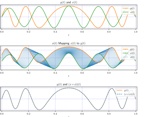
Figure 1: Top. $x$ and $y$. Middle. $\phi$. Bottom. $\tilde{x}$ and $y$.

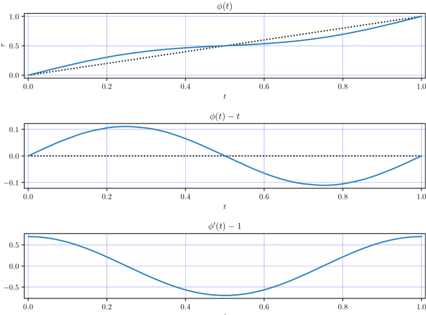
Figure 2: Top. $\phi(t)$. Middle. $\phi(t)-t$. Bottom. $\phi^{\prime}(t)-1$.

Example.

An example is shown in figure 1. The top plot shows a scalar signal $x$ and target signal $y$, and the bottom plot shows the time-warped signal $\tilde{x}=x\circ\phi$ and $y$. The middle plot shows the correspondence between $x$ and $y$ associated with the warping function $\phi$. Figure 2 shows the time warping function; the next plot is the cumulative warp, and the next is the instantaneous rate of time warping.

3 Optimization formulation

We will formulate the dynamic time warping problem as an optimization problem, where the time warp function $\phi$ is the (infinite-dimensional) optimization variable to be chosen. Our formulation is very similar to those used in machine learning, where a fitting function is chosen to minimize an objective that includes a loss function that measures the error in fitting the given data, and regularization terms that penalize the complexity of the fitting function [18].

Loss functional.

Let $L:{\mbox{\bf R}}^{d}\to{\mbox{\bf R}}$ be a vector penalty function. We define the loss associated with a time warp function $\phi$, on the two signals $x$ and $y$, as

$$\mathcal{L}(\phi)=\int_{0}^{1}L(x(\phi(t))-y(t)){\hskip 1.0ptdt},$$ (1)

the average value of the penalty function of the difference between the time-warped first signal and the second signal. The smaller $\mathcal{L}(\phi)$ is, the better we consider $\tilde{x}=x\circ\phi$ to approximate $y$.

Simple choices of the penalty include $L(u)=\|u\|_{2}^{2}$ or $L(u)=\|u\|_{1}$. The corresponding losses are the mean-square deviation and mean-absolute deviation, respectively. One useful variation is the Huber penalty [19, 20],

$$L(u)=\left\{\begin{array}[]{ll}\|u\|_{2}^{2}&\|u\|_{2}\leq M\\ 2M\|u\|_{2}-M^{2}&\|u\|_{2}>M,\end{array}\right.$$

where $M>0$ is a parameter. The Huber penalty coincides with the least squares penalty for small $u$, but grows more slowly for $u$ large, and so is less sensitive to outliers. Many other choices are possible, for example

$$L(u)=\left\{\begin{array}[]{ll}0&\|u\|\leq\epsilon\\ 1&\mbox{otherwise},\end{array}\right.$$

where $\epsilon$ is a positive parameter. The associated loss $\mathcal{L}(\phi)$ is the fraction of time the time-warped signal is farther than $\epsilon$ from the second signal (measured by the norm $\|\cdot\|$).

The choice of penalty function $L$ (and therefore loss functional $\mathcal{L}$) will influence the warping found, and should be chosen to capture the notion of approximation appropriate for the given application.

Cumulative warp regularization functional.

We express our desired qualities for or requirements on the time warp function using a regularization functional for the cumulative warp,

$$\mathcal{R}^{\mathrm{cum}}(\phi)=\int_{0}^{1}R^{\mathrm{cum}}(\phi(t)-t){\hskip 1.0ptdt},$$ (2)

where $R^{\mathrm{cum}}:{\mbox{\bf R}}\to{\mbox{\bf R}}\cup\{\infty\}$ is a penalty function on the cumulative warp. The function $R^{\mathrm{cum}}$ can take on the value $+\infty$, which allows us to encode constraints on $\phi$. While we do not require it, we typically have $R^{\mathrm{cum}}(0)=0$, i.e., there is no cumulative regularization cost when the warped time and true time are the same.

Instantaneous warp regularization functional.

The regularization functional for the instantaneous warp is

$$\mathcal{R}^{\mathrm{inst}}(\phi)=\int_{0}^{1}R^{\mathrm{inst}}(\phi^{\prime}(t)-1){\hskip 1.0ptdt},$$ (3)

where $R^{\mathrm{inst}}:{\mbox{\bf R}}\to{\mbox{\bf R}}\cup\{\infty\}$ is the penalty function on the instantaneous rate of time warping. Like the function $R^{\mathrm{cum}}$, $R^{\mathrm{inst}}$ can take on the value $+\infty$, which allows us to encode constraints on $\phi^{\prime}$. By assigning $R^{\mathrm{inst}}(u)=+\infty$ for $u<s^{\mathrm{min}}$, for example, we require that $\phi^{\prime}(t)\geq s^{\mathrm{min}}$ for all $t$. We will assume that this is the case for some positive $s^{\mathrm{min}}$, which ensures that $\phi$ is invertible. While we do not require it, we typically have $R^{\mathrm{inst}}(0)=0$, i.e., there is no instantaneous regularization cost when the instantaneous rate of time warping is one.

As a simple example, we might choose

$$R^{\mathrm{cum}}(u)=u^{2},\qquad R^{\mathrm{inst}}(u)=\left\{\begin{array}[]{ll}u^{2}&s^{\mathrm{min}}\leq u\leq s^{\mathrm{max}}\\ \infty&\mbox{otherwise},\end{array}\right.$$

i.e., a quadratic penalty on cumulative warping, and a square penalty on instantaneous warping, plus the constraint that the slope of $\phi$ must be between $s^{\mathrm{min}}$ and $s^{\mathrm{max}}$. A very wide variety of penalties can be used to express our wishes and requirements on the warping function.

Dynamic time warping via regularized loss minimization.

We propose to choose $\phi$ by solving the optimization problem

$$\begin{array}[]{ll}\mbox{minimize}&f(\phi)=\mathcal{L}(\phi)+\lambda^{\mathrm{cum}}\mathcal{R}^{\mathrm{cum}}(\phi)+\lambda^{\mathrm{inst}}\mathcal{R}^{\mathrm{inst}}(\phi)\\ \mbox{subject to}&\phi(0)=0,\quad\phi(1)=1,\end{array}$$ (4)

where $\lambda^{\mathrm{cum}}$ and $\lambda^{\mathrm{inst}}$ are positive hyper-parameters used to vary the relative weight of the three terms. The variable in this optimization problem is the time warp function $\phi$.

Optimal control formulation.

The problem (4) is an infinite-dimensional, and generally non-convex, optimization problem. Such problems are generally impractical to solve exactly, but we will see that this particular problem can be efficiently and practically solved.

It can be formulated as a classical continuous-time optimal control problem [21], with scalar state $\phi(t)$ and action or input $u(t)=\phi^{\prime}(t)$:

$$\begin{array}[]{ll}\mbox{minimize}&\int_{0}^{1}\left(\ell(\phi(t),u(t),t)+\lambda^{\mathrm{inst}}R^{\mathrm{inst}}(u(t))\right){\hskip 1.0ptdt}\\ \mbox{subject to}&\phi(0)=0,\quad\phi(1)=1,\quad\phi^{\prime}(t)=u(t),\quad 0\leq t\leq 1,\end{array}$$ (5)

where $\ell$ is the state-action cost function

$$\ell(u,v,t)=L(x(u)-y(t))+\lambda^{\mathrm{cum}}R^{\mathrm{cum}}(u).$$

There are many classical methods for numerically solving the optimal control problem (5), but these generally make strong assumptions about the loss and regularization functionals (such as smoothness), and do not solve the problem globally. We will instead solve (5) by brute force dynamic programming, which is practical since the state has dimension one, and so can be discretized.

Lasso and ridge regularization.

Before describing how we solve the optimal control problem (5), we mention two types of regularization that are widely used in machine learning, and what types of warping functions typically result when using them. They correspond to $R^{\mathrm{cum}}$ and $R^{\mathrm{inst}}$ being either $u^{2}$ (quadratic, ridge, or Tikhonov regularization [11, 22]) or $|u|$ (absolute value, $\ell_{1}$ regularization, or Lasso [23, p564] [12])

With $R^{\mathrm{cum}}(u)=u^{2}$, the regularization discourages large deviations between $\tau$ and $t$, but the not the rate at which $\tau$ changes with $t$. With $R^{\mathrm{inst}}(u)=u^{2}$, the regularization discourages large instantaneous warping rates. The larger $\lambda^{\mathrm{cum}}$ is, the less $\tau$ deviates from $t$; the larger $\lambda^{\mathrm{inst}}$ is, the more smooth the time warping function $\phi$ is.

Using absolute value regularization is more interesting. It is well known in machine learning that using absolute value or $\ell_{1}$ regularization leads to solutions with an argument of the absolute value that is sparse, that is, often zero [20]. When $R^{\mathrm{cum}}$ is the absolute value, we can expect many times when $\tau=t$, that is, the warped time and true time are the same. When $R^{\mathrm{inst}}$ is the absolute value, we can expect many times when $\phi^{\prime}(t)=1$, that is, the instantaneous rate of time warping is zero. Typically these regions grow larger as we increase the hyper-parameters $\lambda^{\mathrm{cum}}$ and $\lambda^{\mathrm{inst}}$.

Discretized time formulation.

To solve the problem (4) we discretize time with the $N$ values

$$0=t_{1}<t_{2}<\cdots<t_{N}=1.$$

We will assume that $\phi$ is piecewise linear with knot points at $t_{1},\ldots,t_{N}$; to describe it we only need to specify the warp values $\tau_{i}=\phi(t_{i})$ for $i=1,\ldots,N$, which we express as a vector $\tau\in{\mbox{\bf R}}^{N}$. We assume that the points $t_{i}$ are closely enough spaced that the restriction to piecewise linear form is acceptable. The values $t_{i}$ could be taken as the values at which the signal $y$ is sampled (if it is given by samples), or just the default linear spacing, $t_{i}=(i-1)/(N-1)$. The constraints $\phi(0)=0$ and $\phi(1)=1$ are expressed as $\tau_{1}=0$ and $\tau_{N}=1$.

Using a simple Riemann approximation of the integrals and the approximation

$$\phi^{\prime}(t_{i})=\frac{\phi(t_{i+1})-\phi(t_{i})}{t_{i+1}-t_{i}}=\frac{\tau_{i+1}-\tau_{i}}{t_{i+1}-t_{i}},\quad i=1,\ldots,N-1,$$

we obtain the discretized objective

$$\hat{f}(\tau)=\sum_{i=1}^{N-1}(t_{i+1}-t_{i})\left(L(x(\tau_{i})-y(t_{i}))+\lambda^{\mathrm{cum}}R^{\mathrm{cum}}(\tau_{i}-t_{i})+\lambda^{\mathrm{inst}}R^{\mathrm{inst}}\left(\frac{\tau_{i+1}-\tau_{i}}{t_{i+1}-t_{i}}\right)\right).$$ (6)

The discretized problem is to choose the vector $\tau\in{\mbox{\bf R}}^{N}$ that minimizes $\hat{f}(\tau)$, subject to $\tau_{1}=0$, $\tau_{N}=1$. We call this vector $\tau^{\star}$, with which we can construct an approximation to function $\phi$ using piecewise-linear interpolation. The only approximation here is the discretization; we can use standard techniques based on bounds on derivatives of the functions involved to bound the deviation between the continuous-time objective $f(\phi)$ and its discretized approximation $\hat{f}(\tau)$.

4 Dynamic programming with refinement

In this section we describe a simple method to minimize $\hat{f}(\tau)$ subject to $\tau_{1}=0$ and $\tau_{N}=1$, i.e., to solve the optimal control problem (5) to obtain $\tau^{*}$. We first discretize the possible values of $\tau_{i}$, whereupon the problem can be expressed as a shortest path problem on a graph, and then efficiently and globally solved using standard dynamic programming techniques. To reduce the error associated with the discretization of the values of $\tau_{i}$, we choose a new discretization with the same number of values, but in a reduced range (and therefore, more finely spaced values) around the previously found values. This refinement converges in a few steps to a highly accurate solution of the discretized problem. Subject only to the reasonable assumption that the discretization of the original time and warped time are sufficiently fine, this method finds the global solution.

4.1 Dynamic programming

We now discretize the values that $\tau_{i}$ is allowed to take:

$$\tau_{i}\in\mathcal{T}_{i}=\{\tau_{i1},\ldots,\tau_{iM}\},\quad i=1,\ldots,N.$$

One choice for these discretized values is linear spacing between given lower and upper bounds on $\tau_{i}$, $0\leq l_{i}\leq u_{i}\leq 1$:

$$\tau_{ij}=l_{i}+\frac{j-1}{M-1}(u_{i}-l_{i}),\quad j=1,\ldots,M,\quad i=1,\ldots,N.$$

Here $M$ is the number of values that we use to discretize each value of $\tau_{i}$ (which we take to be the same for each $i$, for simplicity). We will assume that $0\in\mathcal{T}_{1}$ and $1\in\mathcal{T}_{N}$, so the constraints $\tau_{1}=0$ and $\tau_{N}=1$ are feasible.

The bounds can be chosen as

$$l_{i}=\max\{s^{\mathrm{min}}t_{i},1-s^{\mathrm{max}}(1-t_{i})\},\quad u_{i}=\min\{s^{\mathrm{max}}t_{i},1-s^{\mathrm{min}}(1-t_{i})\},\quad i=1,\ldots,N,$$ (7)

where $s^{\mathrm{min}}$ and $s^{\mathrm{max}}$ are the given minimum and maximum allowed values of $\phi^{\prime}$. This is illustrated in figure 3, where the nodes of $\mathcal{T}$ are drawn at position $(t_{i},\tau_{ij})$, for $N=30,M=20$ and various values of $s^{\mathrm{min}}$ and $s^{\mathrm{max}}$. Note that since $\frac{N}{M}$ is the minimum slope, $M$ should be chosen to satisfy $M<\frac{N}{s^{\mathrm{max}}}$, a consideration that is automated in the provided software.

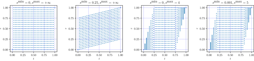
Figure 3: Left. Unconstrained grid. Left center. Effect of introducing $s^{\mathrm{min}}$. Right center. Effect of $s^{\mathrm{max}}$. Right. Typical parameters that work well for our method.

The objective (6) splits into a sum of terms that are functions of $\tau_{i}$, and terms that are functions of $\tau_{i+1}-\tau_{i}$. (These correspond to the separable state-action loss function terms in the optimal control problem associated with $\phi(t)$ and $\phi^{\prime}(t)$, respectively.) The problem is then globally solved by standard methods of dynamic programming [24], using the methods we now describe.

We form a graph with $MN$ nodes, associated with the values $\tau_{ij}$, $i=1,\ldots,N$ and $j=1,\ldots,M$. (Note that $i$ indexes the discretized values of $t$, and $j$ indexes the discretized values of $\tau$.) Each node $\tau_{ij}$ with $i<N$ has $M$ outgoing edges that terminate at the nodes of the form $\tau_{i+1,k}$ for $k=1,\ldots,M$. The total number of edges is therefore $(N-1)M^{2}$. This is illustrated in figure 3 for $M=25$ and $N=100$, where the nodes are shown at the location $(t_{i},\tau_{ij})$. (In practice $M$ and $N$ would be considerably larger.)

At each node $\tau_{ij}$ we associate the node cost

$$L(x(\tau_{ij})-y(t_{i}))+\lambda^{\mathrm{cum}}R^{\mathrm{cum}}(\tau_{ij})$$

and on the edge from $\tau_{ij}$ to $\tau_{i+1,k}$ we associate the edge cost

$$\lambda^{\mathrm{inst}}R^{\mathrm{inst}}\left(\frac{\tau_{i+1,k}-\tau_{ij}}{t_{i+1}-t_{i}}\right).$$

With these node and edge costs, the objective $\hat{f}(\tau)$ is the total cost of a path starting at node $\tau_{11}=0$ and ending at $\tau_{NM}=1$. (Infeasible paths, for examples ones for which $\tau_{i+1,k}<\tau_{i,j}$, have cost $+\infty$.) Our problem is therefore to find the shortest weighted path through a graph, which is readily done by dynamic programming.

The computational cost of dynamic programming is order $NM^{2}$ flops (not counting the evaluation of the loss and regularization terms). With current hardware, it is entirely practical for $M=N=1000$ or even (much) larger. The path found is the globally optimal one, i.e., $\tau^{*}$ minimizes $\hat{f}(\tau)$, subject to the discretization constraints on the values of $\tau_{i}$.

4.2 Iterative refinement

After solving the problem above by dynamic programming, we can reduce the error induced by discretizing the values of $\tau_{i}$ by updating $l_{i}$ and $u_{i}$. We shrink them both toward the current value of $\tau^{*}_{i}$, thereby reducing the gap between adjacent discretized values and reducing the discretization error. One simple method for updating the bounds is to reduce the range $u_{i}-l_{i}$ by a fixed fraction $\eta$, say $1/2$ or $1/8$.

To do this we set

$$l_{i}^{(q+1)}=\max\{\tau^{*(q)}_{i}-\eta\frac{u_{i}^{(q)}-l_{i}^{(q)}}{2},l_{i}^{(0)}\},\qquad u_{i}^{(q+1)}=\min\{\tau^{*(q)}_{i}+\eta\frac{u_{i}^{(q)}-l_{i}^{(q)}}{2},u_{i}^{(0)}\}$$

in iteration $q+1$, where the superscripts in parentheses above indicate the iteration. Using the same data as figure 2, figure 4 shows the iterative refinement of $\tau^{*}$. Here, nodes of $\mathcal{T}$ are plotted at position $(t_{i},\tau_{ij})$, as it is iteratively refined around $\tau^{*}_{i}$.

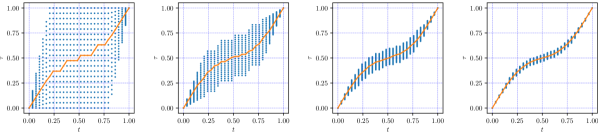
Figure 4: Left to right. Iterative refinement of $\tau^{*}$ for iterations $q=0,1,2,3$, with $\tau^{*}$ colored orange.

4.3 Implementation

GDTW package.

The algorithm described above has been implemented as the open source Python package GDTW, with the dynamic programming portion written in C++ for improved efficiency. The node costs are computed and stored in an $M\times N$ array, and the edge costs are computed on the fly and stored in an $M\times M\times N$ array. For multiple iterations on group-level alignments (see §7), multi-threading is used to distribute the program onto worker threads.

Performance.

We give an example of the performance attained by GDTW using real-world signals described in §5, which are uniformly sampled with $N=1000$. Although it has no effect on method performance, we take square loss, square cumulative warp regularization, and square instantaneous warp regularization. We take $M=100$.

The computations are carried on a 4 core MacBook. To compute the node costs requires 0.0055 seconds, and to compute the shortest path requires 0.0832 seconds. With refinement factor $\eta=.15$, only three iterations are needed before no significant improvement is obtained, and the result is essentially the same with other choices for the algorithm parameters $N$, $M$, and $\eta$. Over 10 trials, our method only took an average of 0.25 seconds, a 50x speedup over FastDTW, which took an average of 14.1 seconds to compute using a radius of 50, which is equivalent to $M=100$. All of the data and example code necessary to reproduce these results are available in the GDTW repository. Also available are supplementary materials that contain step-by-step instructions and demonstrations on how to reproduce these results.

4.4 Validation

To test the generalization ability of a specific time warping model, parameterized by $L,\lambda^{\mathrm{cum}},R^{\mathrm{cum}},\lambda^{\mathrm{inst}},$ and $R^{\mathrm{inst}}$, we use out-of-sample validation by randomly partitioning $N$ discretized time values $0=t_{1},\ldots,t_{N}=1$ into two sorted ordered sets that contain the boundaries, $t^{\mathrm{train}}\cup\{0,1\}$ and $t^{\mathrm{test}}\cup\{0,1\}$. Using only the time points in $t^{\mathrm{train}}$, we obtain our time warping function $\phi$ by minimizing our discretized objective (6). (Recall that our method does not require signals to be sampled at regular intervals, and so will work with the irregularly spaced time points in $t^{\mathrm{train}}$.)

We compute two loss values: a training error

$$\ell^{\mathrm{train}}=\sum_{i=1}^{|t^{\mathrm{train}}|-1}(t^{\mathrm{train}}_{i+1}-t^{\mathrm{train}}_{i})\left(L(x(\phi(t^{\mathrm{train}}_{i}))-y(t^{\mathrm{train}}_{i}))\right),$$

and a test error

$$\ell^{\mathrm{test}}=\sum_{i=1}^{|t^{\mathrm{test}}|-1}(t^{\mathrm{test}}_{i+1}-t^{\mathrm{test}}_{i})\left(L(x(\phi(t^{\mathrm{test}}_{i}))-y(t^{\mathrm{test}}_{i}))\right).$$

Figure 5 shows $\ell^{\mathrm{test}}$ over a grid of values of $\lambda^{\mathrm{cum}}$ and $\lambda^{\mathrm{inst}}$, for a partition where $t^{\mathrm{train}}$ and $t^{\mathrm{test}}$ each contain $~{}50\%$ of the time points. In this example, we use the signals shown figure 1.

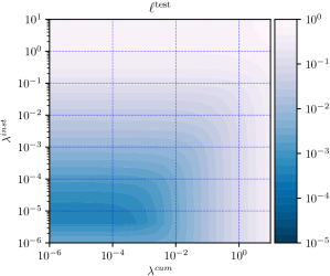
Figure 5: Test loss.

Ground truth estimation.

When a ground truth warping function, $\phi^{\mathrm{true}}$, is available, we can score how well our $\phi$ approximates $\phi^{\mathrm{true}}$ by computing the following errors:

$$\epsilon^{\mathrm{train}}=\sum_{i=1}^{|t^{\mathrm{train}}|-1}(t^{\mathrm{train}}_{i+1}-t^{\mathrm{train}}_{i})\left(L(\phi^{\mathrm{true}}(t^{\mathrm{train}}_{i})-\phi(t^{\mathrm{train}}_{i}))\right),$$

and

$$\epsilon^{\mathrm{test}}=\sum_{i=1}^{|t^{\mathrm{test}}|-1}(t^{\mathrm{test}}_{i+1}-t^{\mathrm{test}}_{i})\left(L(\phi^{\mathrm{true}}(t^{\mathrm{test}}_{i})-\phi(t^{\mathrm{test}}_{i}))\right).$$

In the example shown in figure 5, target signal $y$ is constructed by composing $x$ with a known warping function $\phi^{\mathrm{true}}$, such that $y(t)=(x\circ\phi^{\mathrm{true}})(t)$. Figure 6 shows the contours of $\epsilon^{\mathrm{test}}$ for this example.

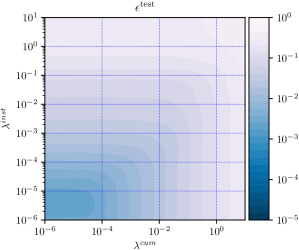
Figure 6: Test error.

5 Examples

We present a few examples of alignments using our method. Figure 7 is a synthetic example of different types of time warping functions. Figure 8 is real-world example using biological signals (ECGs). We compare our method using varying amounts of regularization $\lambda^{\mathrm{inst}}\in\{0.01,0.1,0.5\},N=1000,M=100$ to those using with FastDTW [17], as implemented in the Python package FastDTW [25] using the equivalent graph size $N=1000,\mathrm{radius}=50$. As expected, the alignments using regularization are smoother and less prone to singularities than those from FastDTW, which are unregularized. Figure 9 shows how the time warp functions become smoother as $\lambda^{\mathrm{inst}}$ grows.

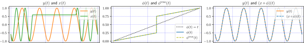
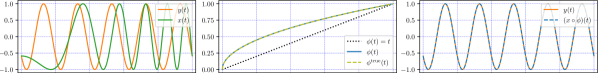
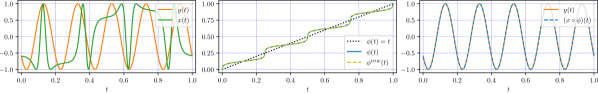
Figure 7: Left. Signal $x$ and target signal $y$. Middle. Warping function $\phi$ and the ground truth warping $\phi^{\mathrm{true}}$. Right. The time-warped $x$ and $y$.

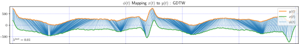
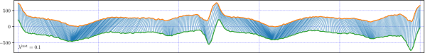
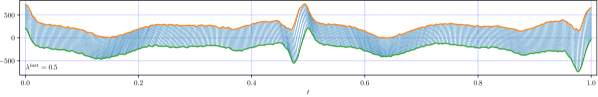
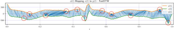
Figure 8: Top four. ECGs warped using our method while increasing $\lambda^{\mathrm{inst}}$. Bottom. Results using FastDTW, with a few of the singularities circled in red.

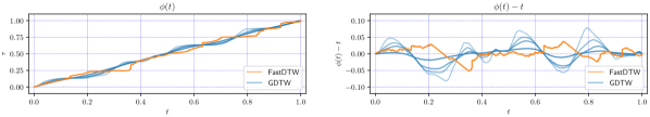
Figure 9: Left. $\phi(t)$ Right. $\phi(t)-t$ for ECGs. (Smoother lines correspond to larger $\lambda^{\mathrm{inst}}$.)

6 Extensions and variations

We will show how to extend our formulation to address complex scenarios, such as aligning a portion of a signal to the target, regularization of higher-order derivatives, and symmetric time warping, where both signals align to each other.

6.1 Alternate boundary and slope constraints

We can align a portion of a signal with the target by adjusting the boundary constraints to allow $0\geq\phi(0)\geq\beta$ and $(1-\beta)\leq\phi(1)\leq 1$, for margin $\beta=\{x\in{\mbox{\bf R}}\ |\ 0<x<1\}$. We incorporate this by reformulating (7) as

$$l_{i}=\max\{s^{\mathrm{min}}t_{i},(1-s^{\mathrm{max}}(1-t_{i}))-\beta\},\quad u_{i}=\min\{s^{\mathrm{max}}t_{i}+\beta,1-s^{\mathrm{min}}(1-t_{i})\},\quad i=1,\ldots,N.$$

We can also allow the slope of $\phi$ to be negative, by choosing $s^{\mathrm{min}}<0$. These modifications are illustrated in figure 10, where the nodes of $\mathcal{T}$ are drawn at position $(t_{i},\tau_{ij})$, for $N=30,M=20$ and various values of $\beta$, $s^{\mathrm{min}}$, and $s^{\mathrm{max}}$.

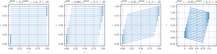
Figure 10: Left. Effect of introducing $\beta$ to unconstrained grid. Left center. Effect of introducing $\beta$ using typical parameters. Right center. Effect of introducing $\beta$ using larger $s^{\mathrm{min}}$. Right. Effect of negative $s^{\mathrm{min}}$.

6.2 Penalizing higher-order derivatives

We can extend the formulation to include a constraint or objective term on the higher-order derivatives, such as the second derivative $\phi^{\prime\prime}$. This requires us to extend the discretized state space to include not just the current $M$ values, but also the last $M$ values, so the state space size grows to $M^{2}$ in the dynamic programming problem.

The regularization functional for the second-order instantaneous warp is

$$\mathcal{R}^{\mathrm{inst^{2}}}(\phi)=\int_{0}^{1}R^{\mathrm{inst^{2}}}(\phi^{\prime\prime}(t)){\hskip 1.0ptdt},$$

where $R^{\mathrm{inst^{2}}}:{\mbox{\bf R}}\to{\mbox{\bf R}}\cup\{\infty\}$ is the penalty function on the second-order instantaneous rate of time warping. Like the function $R^{\mathrm{inst}}$, $R^{\mathrm{inst^{2}}}$ can take on the value $+\infty$, which allows us to encode constraints on $\phi^{\prime\prime}$.

We use a three-point central difference approximation of the second derivative for evenly spaced time points

$$\phi^{\prime\prime}(t_{i})=\frac{\phi(t_{i+1})-2\phi(t_{i})+\phi(t_{i-1})}{(t_{i+1}-t_{i})^{2}}=\frac{\tau_{i+1}-2\tau_{i}+\tau_{i-1}}{(t_{i+1}-t_{i})^{2}},\quad i=1,\ldots,N-1,$$

and unevenly spaced time points

$$\phi^{\prime\prime}(t_{i})=\frac{2(\delta_{1}\phi(t_{i+1})-(\delta_{1}+\delta_{2})\phi(t_{i})+\delta_{2}\phi(t_{i-1}))}{\delta_{1}\delta_{2}(\delta_{1}+\delta_{2})}=\frac{2(\delta_{1}\tau_{i+1}-(\delta_{1}+\delta_{2})\tau_{i}+\delta_{2}\tau_{i-1})}{\delta_{1}\delta_{2}(\delta_{1}+\delta_{2})},$$

for $i=1,\ldots,N-1$, where $\delta_{1}=t_{i}-t_{i-1}$ and $\delta_{2}=t_{i+1}-t_{i}$. With this approximation, we obtain the discretized objective

$$\hat{f}(\tau)=\sum_{i=1}^{N-1}(t_{i+1}-t_{i})\left(L(x(\tau_{i})-y(t_{i}))+\lambda^{\mathrm{cum}}R^{\mathrm{cum}}(\tau_{i}-t_{i})+\lambda^{\mathrm{inst}}R^{\mathrm{inst}}(\phi^{\prime}(t_{i}))+\lambda^{\mathrm{inst^{2}}}R^{\mathrm{inst^{2}}}(\phi^{\prime\prime}(t_{i}))\right).$$

6.3 General loss

The two signals need not be vector valued; they could have categorical values, for example

$$L(\tau_{i},t_{i})=\left\{\begin{array}[]{ll}1&\tau_{i}\neq t_{i}\\ 0&\mbox{otherwise},\end{array}\right.$$

or

$$L(\tau_{i},t_{i})=\left\{\begin{array}[]{ll}g(\tau_{i},t_{i})&\tau_{i}\neq t_{i}\\ 0&\mbox{otherwise},\end{array}\right.$$

where $g:{\mbox{\bf R}}_{++}\times{\mbox{\bf R}}_{++}\to{\mbox{\bf R}}$ is a categorical distance function that can specify the cost of certain mismatches or a similarity matrix [26].

Another example could use the Earth mover’s distance, $\mbox{EMD}:{\mbox{\bf R}}^{n}\times{\mbox{\bf R}}^{n}\to{\mbox{\bf R}}$, between two short-time spectra

$$L(\phi,t_{i})=\mbox{EMD}(\{\phi(t_{i}-\rho),\ldots,\phi(t_{i}),\ldots,\phi(t_{i}+\rho)\},\{t_{i}-\rho,\ldots,t_{i},\ldots,t_{i}+\rho\}),$$

where $\rho\in{\mbox{\bf R}}$ is a radius around time point $t_{i}$.

6.4 Symmetric time warping

Until this point, we have used unidirectional time warping, where signal $x$ is time-warped to align with $y$ such that $x\circ\phi\approx y$. We can also perform bidirectional time warping, where signals $x$ and $y$ are time-warped each other. Bidirectional time warping results in two time warp functions, $\phi$ and $\psi$, where $x\circ\phi\approx y\circ\psi$.

Bidirectional time warping requires a different loss functional. Here we define the bidirectional loss associated with time warp functions $\phi$ and $\psi$, on the two signals $x$ and $y$, as

$$\mathcal{L}(\phi,\psi)=\int_{0}^{1}L(x(\phi(t))-y(\psi(t))){\hskip 1.0ptdt},$$

where we distinguish the bidirectional case by using two arguments, $\mathcal{L}(\phi,\psi)$, instead of one, $\mathcal{L}(\phi)$, as in (1).

Bidirectional time warping can be symmetric or asymmetric. In the symmetric case, we choose $\phi,\psi$ by solving the optimization problem

$$\begin{array}[]{ll}\mbox{minimize}&\mathcal{L}(\phi,\psi)+\lambda^{\mathrm{cum}}\mathcal{R}^{\mathrm{cum}}(\phi)+\lambda^{\mathrm{inst}}\mathcal{R}^{\mathrm{inst}}(\phi)\\ \mbox{subject to}&\phi(0)=0,\quad\phi(1)=1,\quad\psi(t)=2t-\phi(t),\end{array}$$

where the constraint $\psi(t)=2t-\phi(t)$ ensures that $\phi$ and $\psi$ are symmetric about the identity. The symmetric case does not add additional computational complexity, and can be readily solved using the iterative refinement procedure described in §4.

In the asymmetric case, $\phi,\psi$ are chosen by solving the optimization problem

$$\begin{array}[]{ll}\mbox{minimize}&\mathcal{L}(\phi,\psi)+\lambda^{\mathrm{cum}}\mathcal{R}^{\mathrm{cum}}(\phi)+\lambda^{\mathrm{cum}}\mathcal{R}^{\mathrm{cum}}(\psi)+\lambda^{\mathrm{inst}}\mathcal{R}^{\mathrm{inst}}(\phi)+\lambda^{\mathrm{inst}}\mathcal{R}^{\mathrm{inst}}(\psi)\\ \mbox{subject to}&\phi(0)=0,\quad\phi(1)=1,\quad\psi(0)=0,\quad\psi(1)=1.\end{array}$$

The asymmetric case requires $R^{\mathrm{cum}}$, $R^{\mathrm{inst}}$ to allow negative slopes for $\psi$. Further, it requires a modified iterative refinement procedure (not described here) with an increased complexity of order $NM^{4}$ flops, which is impractical when $M$ is not small.

7 Time-warped distance, centering, and clustering

In this section we describe three simple extensions of our optimization formulation that yield useful methods for analyzing a set of signals $x_{1},\ldots,x_{M}$.

7.1 Time-warped distance

For signals $x$ and $y$, we can interpret the optimal value of (4) as the time-warped distance between $x$ and $y$, denoted $D(x,y)$. (Note that this distance measures takes into account both the loss and the regularization, which measures how much warping was needed.) When $\lambda^{\mathrm{cum}}$ and $\lambda^{\mathrm{inst}}$ are zero, we recover the unconstrained DTW distance [1]. This distance is not symmetric; we can (and usually do) have $D(x,y)\neq D(y,x)$. If a symmetric distance is preferred, we can take $(D(x,y)+D(y,x))/2$, or the optimal value of the group alignment problem (8), with a set of original signals $x,y$.

The warp distance can be used in many places where a conventional distance between two signals is used. For example we can use warp distance to carry out $k$ nearest neighbors regression [27] or classification. Warp distance can also be used to create features for further machine learning. For example, suppose that we have carried out clustering into $K$ groups, as discussed above, with target or group centers or exemplar signals $y_{1},\ldots,y_{K}$. From these we can create a set of $K$ features related to the warp distance of a new signal $x$ to the centers $y_{1},\ldots,y_{K}$, as

$$z_{i}=\frac{e^{d_{i}/\sigma}}{\sum_{j=1}^{K}e^{d_{j}/\sigma}},\quad i=1,\ldots,K,$$

where $d_{i}=D(x,y_{i})$ and $\sigma$ is a positive (scale) hyper-parameter.

7.2 Time-warped alignment and centering

In time-warped alignment, the goal is to find a common target signal $\mu$ that each of the original signals can be warped to, at low cost. We pose this in the natural way as the optimization problem

$$\begin{array}[]{ll}\mbox{minimize}&\sum_{i=1}^{M}\left(\int_{0}^{1}L(x_{i}(\phi_{i}(t))-\mu(t))\;dt+\lambda^{\mathrm{cum}}\mathcal{R}^{\mathrm{cum}}(\phi_{i})+\lambda^{\mathrm{inst}}\mathcal{R}^{\mathrm{inst}}(\phi_{i})\right)\\ \mbox{subject to}&\phi_{i}(0)=0,\quad\phi_{i}(1)=1,\end{array}$$ (8)

where the variables are the warp functions $\phi_{1},\ldots,\phi_{M}$ and the target $\mu$, and $\lambda^{\mathrm{cum}}$ and $\lambda^{\mathrm{inst}}$ are positive hyper-parameters. The objective is the sum of the objectives for time warping each $x_{i}$ to $\mu$. This is very much like our basic formulation (4), except that we have multiple signals to warp, and the target $\mu$ is also a variable that we can choose.

The problem (8) is hard to solve exactly, but a simple iterative procedure seems to work well. We observe that if we fix the target $\mu$, the problem splits into $M$ separate dynamic time warping problems that we can solve (separately, in parallel) using the method described in §4. Conversely, if we fix the warping functions $\phi_{1},\ldots,\phi_{M}$, we can optimize over $\mu$ by minimizing

$$\sum_{i=1}^{M}\int_{0}^{1}L(x_{i}(\phi_{i}(t))-\mu(t))\;dt.$$

This is turn amounts to choosing each $\mu(t)$ to minimize

$$\sum_{i=1}^{M}L(x_{i}(\phi_{i}(t))-\mu(t)).$$

This is typically easy to do; for example, with square loss, we choose $\mu(t)$ to be the mean of $x_{i}(\phi_{i}(t))$; with absolute value loss, we choose $\mu(t)$ to be the median of $x_{i}(\phi_{i}(t))$.

This method of alternating between updating the target $\mu$ and updating the warp functions (in parallel) typically converges quickly. However, it need not converge to the global minimum. One simple initialization is to start with no warping, i.e., $\phi_{i}(t)=t$. Another is to choose one of the original signals as the initial value for $\mu$.

As a variation, we can also require the warping functions to be evenly arranged about a common time warp center, for example $\phi(t)=t$. We can do this by imposing a “centering” constraint on (8),

$$\begin{array}[]{ll}\mbox{minimize}&\sum_{i=1}^{M}\left(\int_{0}^{1}L(x_{i}(\phi_{i}(t))-\mu(t))\;dt+\lambda^{\mathrm{cum}}\mathcal{R}^{\mathrm{cum}}(\phi_{i})+\lambda^{\mathrm{inst}}\mathcal{R}^{\mathrm{inst}}(\phi_{i})\right)\\ \mbox{subject to}&\phi_{i}(0)=0,\quad\phi_{i}(1)=1,\quad\frac{1}{M}\sum_{i=1}^{M}\phi_{i}(t)=t,\end{array}$$ (9)

where $\frac{1}{M}\sum_{i=1}^{M}\phi_{i}(t)=t$ forces $\phi_{1},\ldots,\phi_{M}$ to be evenly distributed around the identity $\phi(t)=t$. The resulting centered time warp functions, can be used to produce a centered time-warped mean. Figure 11 compares a time-warped mean with and without centering, using synthetic data consisting of multi-modal signals from [5].

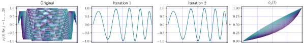
Figure 11: Top. Time-warped mean. Bottom. Centered time-warped mean. Left. Original signals. Left center. Warped signals after iteration 1. Right center. Warped signals after iteration 2. Right. Time warp functions after iteration 2.

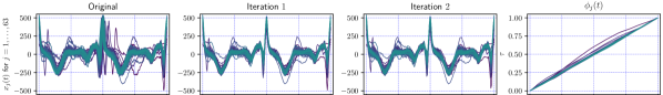
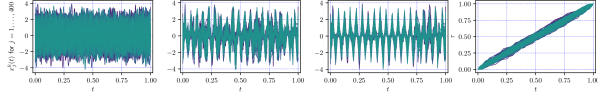
Figure 12: Top. ECG signals. Bottom. Engine sensor signals. Left. Original signals. Left center. Warped signals after iteration 1. Right center. Warped signals after iteration 2. Right. Time warp functions after iteration 2.

Figure 12 shows examples of centered time-warped means of real-world data (using our default parameters), consisting of ECGs and sensor data from an automotive engine [28]. The ECG example demonstrates that subtle features of the input sequences are preserved in the alignment process, and the engine example demonstrates that the alignment process can find structure in noisy data.

7.3 Time-warped clustering

A further generalization of our optimization formulation allows us to cluster set of signals $x_{1},\ldots,x_{M}$ into $K$ groups, with each group having a template or center or exemplar. This can be considered a time-warped version of $K$-means clustering; see, e.g., [29, Chapter 4]. To describe the clusters we use the $M$-vector $c$, with $c_{i}=j$ meaning that signal $x_{i}$ is assigned to group $j$, where $j\in\{1,\ldots,M\}$. The exemplars or templates are the signals denoted $y_{1},\ldots,y_{K}$.

$$\begin{array}[]{ll}\mbox{minimize}&\sum_{i=1}^{M}\left(\int_{0}^{1}L(x_{i}(\phi_{i}(t))-y_{c_{i}}(t))\;dt+\lambda^{\mathrm{cum}}\mathcal{R}^{\mathrm{cum}}(\phi_{i})+\lambda^{\mathrm{inst}}\mathcal{R}^{\mathrm{inst}}(\phi_{i})\right)\\ \mbox{subject to}&\phi_{i}(0)=0,\quad\phi_{i}(1)=1,\end{array}$$ (10)

where the variables are the warp functions $\phi_{1},\ldots,\phi_{M}$, the templates $y_{1},\ldots,y_{K}$, and the assignment vector $c$. As above, $\lambda^{\mathrm{cum}}$ and $\lambda^{\mathrm{inst}}$ are positive hyper-parameters.

We solve this (approximately) by cyclically optimizing over the warp functions, the templates, and the assignments. Figure 13 shows an example of this procedure (using our default parameters) on a set of sinusoidal, square, and triangular signals of varying phase and amplitude.

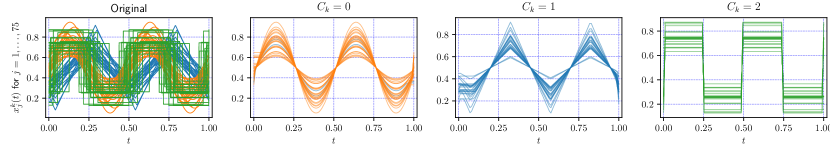
Figure 13: $K$-means alignment on synthetic data.

8 Conclusion

We claim three main contributions. We propose a full reformulation of DTW in continuous time that eliminates singularities without the need for preprocessing or step functions. Because our formulation allows for non-uniformly sampled signals, we are the first to demonstrate how validation can be used for DTW model selection. Finally, we offer an implementation that runs 50x faster than state-of-the-art methods on typical problem sizes, and distribute our C++ code (as well as all of our example data) as an open-source Python package called GDTW.

References

- [1] H. Sakoe and S. Chiba. Dynamic programming algorithm optimization for spoken word recognition. IEEE transactions on acoustics, speech, and signal processing, 26(1):43–49, 1978.
- [2] E. Keogh and M. Pazzani. Derivative dynamic time warping. In Proceedings of the 2001 SIAM International Conference on Data Mining, pages 1–11. SIAM, 2001.
- [3] J. Marron, J. Ramsay, L. Sangalli, and A. Srivastava. Functional data analysis of amplitude and phase variation. Statistical Science, 30(4):468–484, 2015.
- [4] M. Singh, I. Cheng, M. Mandal, and A. Basu. Optimization of symmetric transfer error for sub-frame video synchronization. In European Conference on Computer Vision, pages 554–567. Springer, 2008.
- [5] A. Srivastava, W. Wu, S. Kurtek, E. Klassen, and J. Marron. Registration of functional data using Fisher-Rao metric. arXiv preprint arXiv:1103.3817, 2011.
- [6] M. Dupont and P. Marteau. Coarse-DTW for sparse time series alignment. In International Workshop on Advanced Analytics and Learning on Temporal Data, pages 157–172. Springer, 2015.
- [7] J. Zhao and L. Itti. ShapeDTW: Shape dynamic time warping. arXiv preprint arXiv:1606.01601, 2016.
- [8] F. Itakura. Minimum prediction residual principle applied to speech recognition. IEEE Transactions on Acoustics, Speech, and Signal Processing, 23(1):67–72, 1975.
- [9] C. Myers, L. Rabiner, and A. Rosenberg. Performance tradeoffs in dynamic time warping algorithms for isolated word recognition. IEEE Transactions on Acoustics, Speech, and Signal Processing, 28(6):623–635, 1980.
- [10] L. Rabiner and B. Juang. Fundamentals of Speech Recognition. Prentice Hall, 1993.
- [11] A. Tikhonov and V. Arsenin. Solutions of Ill-Posed Problems, volume 14. Winston, 1977.
- [12] R. Tibshirani. Regression shrinkage and selection via the lasso. Journal of the Royal Statistical Society, 58(1):267–288, 1996.
- [13] P. Green and B. Silverman. Non-Parametric Regression and Generalized Linear Models: A Roughness Penalty Approach. CRC Press, 1993.
- [14] J. Ramsay and B. Silverman. Functional Data Analysis. Springer, 2005.
- [15] J. Ramsay and B. Silverman. Applied Functional Data Analysis: Methods and Case Studies. Springer, 2007.
- [16] A. Srivastava and E. Klassen. Functional and Shape Data Analysis. Springer, 2016.
- [17] S. Salvador and P. Chan. Toward accurate dynamic time warping in linear time and space. Intelligent Data Analysis, 11(5):561–580, 2007.
- [18] J. Friedman, T. Hastie, and R. Tibshirani. The Elements of Statistical Learning, volume 1. Springer, 2001.
- [19] P.J. Huber. Robust statistics. In International Encyclopedia of Statistical Science, pages 1248–1251. Springer, 2011.
- [20] S. Boyd and L. Vandenberghe. Convex Optimization. Cambridge University Press, 2004.
- [21] D. P. Bertsekas. Dynamic Programming and Optimal Control, volume 1. Athena Scientific, 2005.
- [22] P. Hansen. Rank-Deficient and Discrete Ill-Posed Problems: Numerical Aspects of Linear Inversion, volume 4. SIAM, 2005.
- [23] G. Golub and C. Van Loan. Matrix Computations, volume 3. JHU Press, 2012.
- [24] R. Bellman and S. Dreyfus. Applied Dynamic Programming, volume 2050. Princeton University Press, 2015.
- [25] K. Tanida. FastDTW. GitHub Repository https://github.com/slaypni/fastdtw, 2015.
- [26] S. Needleman and C. Wunsch. A general method applicable to the search for similarities in the amino acid sequence of two proteins. Journal of molecular biology, 48(3):443–453, 1970.
- [27] X. Xi, E. Keogh, C. Shelton, L. Wei, and C. A. Ratanamahatana. Fast time series classification using numerosity reduction. In Proceedings of the 23rd international conference on Machine learning, pages 1033–1040. ACM, 2006.
- [28] M. Abou-Nasr and L. Feldkamp. Ford Classification Challenge. Zip Archive http://www.timeseriesclassification.com/description.php?Dataset=FordA, 2008.
- [29] S. Boyd and L. Vandenberghe. Introduction to Applied Linear Algebra: Vectors, Matrices, and Least Squares. Cambridge University Press, 2018.