Multi-Objective Generalized Linear Bandits

Abstract

In this paper, we study the multi-objective bandits (MOB) problem, where a learner repeatedly selects one arm to play and then receives a reward vector consisting of multiple objectives. MOB has found many real-world applications as varied as online recommendation and network routing. On the other hand, these applications typically contain contextual information that can guide the learning process which, however, is ignored by most of existing work. To utilize this information, we associate each arm with a context vector and assume the reward follows the generalized linear model (GLM). We adopt the notion of Pareto regret to evaluate the learner’s performance and develop a novel algorithm for minimizing it. The essential idea is to apply a variant of the online Newton step to estimate model parameters, based on which we utilize the upper confidence bound (UCB) policy to construct an approximation of the Pareto front, and then uniformly at random choose one arm from the approximate Pareto front. Theoretical analysis shows that the proposed algorithm achieves an $\tilde{O}(d\sqrt{T})$ Pareto regret, where $T$ is the time horizon and $d$ is the dimension of contexts, which matches the optimal result for single objective contextual bandits problem. Numerical experiments demonstrate the effectiveness of our method.

1 Introduction

Online learning under bandit feedback is a powerful paradigm for modeling sequential decision-making process arising in various applications such as medical trials, advertisement placement, and network routing Bubeck and Cesa-Bianchi (2012). In the classic stochastic multi-armed bandits (MAB) problem, at each round a learner firstly selects one arm to play and then obtains a reward drawn from a fixed but unknown probability distribution associated with the selected arm. The learner’s goal is to minimize the regret, which is defined as the difference between the cumulative reward of the learner and that of the best arm in hindsight. Algorithms designed for this problem need to strike a balance between exploration and exploitation, i.e., identifying the best arm by trying different arms while spending as much as possible on the seemingly optimal arm.

A natural extension of MAB is the multi-objective multi-armed bandits (MOMAB), proposed by Drugan and Nowe Drugan and Nowe (2013), where the reward pertaining to an arm is a multi-dimensional vector instead of a scalar value. In this setting, different arms are compared according to Pareto order between their reward vectors, and those arms whose rewards are not inferior to that of any other arms are called Pareto optimal arms, all of which constitute the Pareto front. The standard metric is the Pareto regret, which measures the cumulative gap between the reward of the learner and that of the Pareto front. The task here is to design online algorithms that minimize the Pareto regret by judiciously selecting seemingly Pareto optimal arms based on historical observation, while ensuring fairness, that is, treating each Pareto optimal arm as equally as possible. MOMAB is motivated by real-world applications involved with multiple optimization objectives, e.g., novelty and diversity in recommendation systems Rodriguez et al. (2012). On the other hand, the aforementioned real-world applications typically contain auxiliary information (contexts) that can guide the decision-making process, such as user profiles in recommendation systems Li et al. (2010), which is ignored by MOMAB.

To incorporate this information into the decision-making process, Turgay et al. Turgay et al. (2018) extended MOMAB to the multi-objective contextual bandits (MOCB). In MOCB, the learner is endowed with contexts before choosing arms and the reward he receives in each round obeys a distribution whose expectation depends on the contexts and the chosen arm. Turgay et al. Turgay et al. (2018) assumed that the learner has a prior knowledge of the similarity information that relates distances between the context-arm pairs to those between the expected rewards. Under this assumption, they proposed an algorithm called Pareto contextual zooming which is built upon the contextual zooming method Slivkins (2014). However, the Pareto regret of their algorithm is $\tilde{O}(T^{1-1/(2+d_{p})})$, where $d_{p}$ is the Pareto zooming dimension, which is almost linear in $T$ when $d_{p}$ is large (say, $d_{p}=10$) and hence hinders the application of their algorithm to broad domains.

To address this limitation, we formulate the multi-objective contextual bandits under a different assumption—the parameterized realizability assumption, which has been extensively studied in single objective contextual bandits Auer (2002); Dani et al. (2008). Concretely, we model the context associated with an arm as a $d$-dimensional vector $x\in\mathbb{R}^{d}$ and for the sake of clarity denote the arm by $x$. The reward vector $y$ pertaining to an arm $x$ consists of $m$ objectives. The value of each objective is drawn according to the generalized linear model Nelder and Wedderburn (1972) such that

$$\mathbb{E}[y^{i}|x]=\mu_{i}(\theta_{i}^{\top}x),\;i=1,\ldots,m$$

where $y^{i}$ represents the $i$-th component of $y$, $\theta_{1},\ldots,\theta_{m}$ are vectors of unknown coefficients, and $\mu_{1},\ldots,\mu_{m}$ are link functions. We refer to this formulation as multi-objective generalized linear bandits (MOGLB), which is very general and covers a wide range of problems, such as stochastic linear bandits Auer (2002); Dani et al. (2008) and online stochastic linear optimization under binary feedback Zhang et al. (2016), where the link functions are the identity function and the logistic function respectively.

To the best of our knowledge, this is the first work that investigates the generalized linear bandits (GLB) in multi-objective scenarios. Note that a naive application of existing GLB algorithms to a specific objective does not work, because it could favor those Pareto optimal arms that achieve maximal reward in this objective, which harms the fairness. To resolve this problem, we develop a novel algorithm named MOGLB-UCB. Specifically, we employ a variant of the online Newton step to estimate unknown coefficients and utilize the upper confidence bound policy to construct an approximate Pareto front, from which the arm is then pulled uniformly at random. Theoretical analysis shows that the proposed algorithm enjoys a Pareto regret bound of $\tilde{O}(d\sqrt{T})$, where $T$ is the time horizon and $d$ is the dimension of contexts. This bound is sublinear in $T$ regardless of the dimension and matches the optimal regret bound for single objective contextual bandits problem. Empirical results demonstrate that our algorithm can not only minimize Pareto regret but also ensure fairness.

2 Related Work

In this section, we review the related work on stochastic contextual bandits, parameterized contextual bandits, and multi-objective bandits.

2.1 Stochastic Contextual Bandits

In the literature, there exist many formulations of the stochastic contextual bandits, under different assumptions on the problem structure, i.e., the mechanism of context arrivals and the relation between contexts and rewards.

One category of assumption says that the context and reward follow a fixed but unknown joint distribution. This problem is first considered by Langford and Zhang Langford and Zhang (2008), who proposed an efficient algorithm named Epoch-Greedy. However, the regret of their algorithm is $O(T^{2/3})$, which is suboptimal when compared to inefficient algorithms such as Exp4 Auer et al. (2002b). Later on, efficient and optimal algorithms that attain an $\tilde{O}(T^{1/2})$ regret are developed Dudik et al. (2011); Agarwal et al. (2014).

Another line of work Kleinberg et al. (2008); Bubeck et al. (2009); Lu et al. (2010); Slivkins (2014); Lu et al. (2019) assume that the relation between the rewards and the contexts can be modeled by a Lipschitz function. Lu et al. Lu et al. (2010) established an $\Omega(T^{1-1/(2+d_{p})})$ lower bound on regret under this setting and proposed the Query-Ad-Clustering algorithm, which attains an $\tilde{O}(T^{1-1/(2+d_{c})})$ regret, where $d_{p}$ and $d_{c}$ are the packing dimension and the covering dimension of the similarity space respectively. Slivkins Slivkins (2014) developed the contextual zooming algorithm, which enjoys a regret bound of $\tilde{O}(T^{1-1/(2+d_{z})})$, where $d_{z}$ is the zooming dimension of the similarity space.

2.2 Parameterized Contextual Bandits

In this paper, we focus on the parameterized contextual bandits, where each arm is associated with a $d$-dimensional context vector and the expected reward is modeled as a parameterized function of the arm’s context. Auer Auer (2002) considered the linear case of this problem under the name of stochastic linear bandits (SLB) and developed a complicated algorithm called SuperLinRel, which attains an $\tilde{O}(({\log{K}})^{3/2}\sqrt{dT})$ regret, assuming the arm set is finite. Later, Dani et al. Dani et al. (2008) proposed a much simpler algorithm named ConfidenceBall₂, which enjoys a regret bound of $\tilde{O}(d\sqrt{T})$ and can be used for infinite arm set.

Filippi et al. Filippi et al. (2010) extended SLB to the generalized linear bandits, where the expected reward is a composite function of the arm’s context. The inside function is linear and the outside function is certain link function. The authors proposed a UCB-type algorithm that enjoys a regret bound of $\tilde{O}(d\sqrt{T})$. However, their algorithm is not efficient since it needs to store the whole learning history and perform batch computation to estimate the function. Zhang et al. Zhang et al. (2016) studied a particular case of GLB in which the reward is generated by the logit model and developed an efficient algorithm named OL²M, which attains an $\tilde{O}(d\sqrt{T})$ regret. Later, Jun et al. Jun et al. (2017) extended OL²M to generic GLB problems.

2.3 Multi-Objective Bandits

The seminal work of Drugan and Nowe Drugan and Nowe (2013) proposed the standard formulation of the multi-objective multi-armed bandits and introduced the notion of Pareto regret as the performance measure. By making use of the UCB technique, they developed an algorithm that enjoys a Pareto regret bound of $O(\log{T})$. Turgay et al. Turgay et al. (2018) extended MOMAB to the contextual setting with the similarity information assumption. Based on the contextual zooming method Slivkins (2014), the authors proposed an algorithm called Pareto contextual zooming whose Pareto regret is $\tilde{O}(T^{1-1/(2+d_{p})})$, where $d_{p}$ is the Pareto zooming dimension. Another related line of the MOMAB researches Drugan and Nowé (2014); Auer et al. (2016) study the best arm identification problem. The focus of those papers is to identify all Pareto optimal arms within a fixed budget.

3 Multi-Objective Generalized Linear Bandits

We first introduce notations used in this paper, next describe the learning model, then present our algorithm, and finally state its theoretical guarantees.

3.1 Notation

Throughout the paper, we use the subscript to distinguish different objects (e.g., scalars, vectors, functions) and superscript to identify the component of an object. For example, $y_{t}^{i}$ represents the $i$-th component of the vector $y_{t}$. For the sake of clarity, we denote the $\ell_{2}$-norm by $\|\cdot\|$. The induced matrix norm associated with a positive definite matrix $A$ is defined as $\|x\|_{A}\coloneqq\sqrt{x^{\top}Ax}$. We use $\mathcal{B}_{R}\coloneqq\{x~{}|~{}\|x\|\leq R\}$ to denote a centered ball whose radius is $R$. Given a positive semidefinite matrix $P$, the generalized projection of a point $x$ onto a convex set $\mathcal{W}$ is defined as $\Pi_{\mathcal{W}}^{P}[x]\coloneqq\mathop{\arg\min}_{y\in\mathcal{W}}(y-x)^{\top}P(y-x)$. Finally, $[n]\coloneqq\{1,2,\ldots,n\}$.

3.2 Learning Model

We now give a formal description of the learning model investigated in this paper.

3.2.1 Problem Formulation

We consider the multi-objective bandits problem under the GLM realizability assumption. Let $m$ denote the number of objectives and $\mathcal{X}\subset\mathbb{R}^{d}$ be the arm set. In each round $t$, a learner selects an arm $x_{t}\in\mathcal{X}$ to play and then receives a stochastic reward vector $y_{t}\in\mathbb{R}^{m}$ consisting of $m$ objectives. We assume each objective $y_{t}^{i}$ is generated according to the GLM such that for $i=1,2,\ldots,m$,

$$\Pr(y_{t}^{i}|x_{t})=h_{i}(y_{t}^{i},\tau_{i})\exp\left(\frac{y_{t}^{i}\theta_{i}^{\top}x_{t}-g_{i}(\theta_{i}^{\top}x_{t})}{\tau_{i}}\right)$$

where $\tau_{i}$ is the dispersion parameter, $h_{i}$ is a normalization function, $g_{i}$ is a convex function, and $\theta_{i}$ is a vector of unknown coefficients. Let $\mu_{i}=g_{i}^{\prime}$ denote the so-called link function, which is monotonically increasing due to the convexity of $g_{i}$. It is easy to show $\mathbb{E}[y_{t}^{i}|x_{t}]=\mu_{i}(\theta_{i}^{\top}x_{t})$.

A remarkable member of the GLM family is the logit model in which the reward is one-bit, i.e., $y\in\{0,1\}$ Zhang et al. (2016), and satisfies

$$\Pr(y=1|x)=\frac{1}{1+\exp{(-\theta^{\top}x)}}.$$

Another well-known binary model belonging to the GLM is the probit model, which takes the following form

$$\Pr(y=1|x)=\Phi(\theta^{\top}x)$$

where $\Phi(\cdot)$ is the cumulative distribution function of the standard normal distribution.

Following previous studies Filippi et al. (2010); Jun et al. (2017), we make standard assumptions as follows.

Assumption 1

The coefficients $\theta_{1},\ldots,\theta_{m}$ are bounded by $D$, i.e., $\|\theta_{i}\|\leq D,\forall i\in[m]$.

Assumption 2

The radius of the arm set $\mathcal{X}$ is bounded by $1$, i.e., $\|x\|\leq 1,\forall x\in\mathcal{X}$.

Assumption 3

For each $i\in[m]$, the link function $\mu_{i}$ is $L$-Lipschitz on $[-D,D]$ and continuously differentiable on $(-D,D)$. Furthermore, we assume that $\mu_{i}^{\prime}(z)\geq\kappa>0,z\in(-D,D)$ and $|\mu_{i}(z)|\leq U,z\in[-D,D]$.

Assumption 4

There exists a positive constant $R$ such that $|y_{t}^{i}|\leq R,\forall t\in[T],i\in[m]$ holds almost surely.

3.2.2 Performance Metric

According to the properties of the GLM, for any arm $x\in\mathcal{X}$ that is played, its expected reward is a vector of $[\mu_{1}(\theta_{1}^{\top}x),\mu_{2}(\theta_{2}^{\top}x),\ldots,\mu_{m}(\theta_{m}^{\top}x)]\in\mathbb{R}^{m}$. With a slight abuse of notation, we denote it by $\mu_{x}$. We compare different arms by their expected rewards and adopt the notion of Pareto order.

Definition 1 (Pareto order)

Let $u,v\in\mathbb{R}^{m}$ be two vectors.

• $u$ dominates $v$, denoted by $v\prec u$, if and only if $\;\forall i\in[m],v^{i}\leq u^{i}$ and $\exists j\in[m],u^{j}>v^{j}$.

• $v$ is not dominated by $u$, denoted by $v\nprec u$, if and only if $v=u$ or $\;\exists i\in[m],v^{i}>u^{i}$.

• $u$ and $v$ are incomparable, denoted by $u\|v$, if and only if either vector is not dominated by the other, i.e., $u\nprec v$ and $v\nprec u$.

Equipped with the Pareto order, we can now define the Pareto optimal arm.

Definition 2 (Pareto optimality)

Let $x\in\mathcal{X}$ be an arm.

• $x$ is Pareto optimal if and only if its expected reward is not dominated by that of any arm in $\mathcal{X}$, i.e., $\;\forall x^{\prime}\in\mathcal{X},\mu_{x}\nprec\mu_{x}^{\prime}$.

• The set comprised of all Pareto optimal arms is called Pareto front, denoted by $\mathcal{O}^{*}$.

It is clear that all arms in the Pareto front are incomparable. In single objective bandits problem, the standard metric to measure the learner’s performance is regret defined as the difference between the cumulative reward of the learner and that of the optimal arm in hindsight. In order to extend such metric to multi-objective setting, we introduce the notion of Pareto suboptimality gap Drugan and Nowe (2013) to measure the difference between the learner’s reward and that of the Pareto optimal arms.

Definition 3 (Pareto suboptimality gap, PSG)

Let $x$ be an arm in $\mathcal{X}$. Its Pareto suboptimality gap $\Delta x$ is defined as the minimal scalar $\epsilon\geq 0$ such that $x$ becomes Pareto optimal after adding $\epsilon$ to all entries of its expected reward. Formally,

$$\Delta x\coloneqq\inf\;\{\epsilon\;|\;(\mu_{x}+\epsilon)\nprec\mu_{x^{\prime}},\forall x^{\prime}\in\mathcal{X}\}.$$

We evaluate the learner’s performance using the (pseudo) Pareto regret Drugan and Nowe (2013) defined as the cumulative Pareto suboptimality gap of the arms pulled by the learner.

Definition 4 (Pareto regret, PR)

Let $x_{1},x_{2},\ldots,x_{T}$ be the arms pulled by the learner. The Pareto regret is defined as

$$PR(T)\coloneqq\sum_{t=1}^{T}\Delta x_{t}.$$

3.3 Algorithm

The proposed algorithm, termed MOGLB-UCB, is outlined in Algorithm 1. Had we known all coefficients $\theta_{1},\ldots,\theta_{m}$ in advance, we could compute the Pareto front directly and always pull the Pareto optimal arms, whose Pareto suboptimality gaps are zero. Motivated by this observation, we maintain an arm set $\mathcal{O}_{t}$ as an approximation to the Pareto front $\mathcal{O}^{*}$ and always play arms in $\mathcal{O}_{t}$. To encourage fairness, we draw an arm $x_{t}$ from $\mathcal{O}_{t}$ uniformly at random to play (Step 3). The approximate Pareto front is initialized to be $\mathcal{X}$ and is updated as follows.

In each round $t$, after observing the reward vector $y_{t}$, we make an estimation denoted by $\hat{\theta}_{t+1,i}$ for each coefficients $\theta_{i}$ (Steps 4-7). Let $\mathcal{H}_{t}\coloneqq\{(x_{1},y_{1}),(x_{2},y_{2}),\ldots,(x_{t},y_{t})\}$ be the learning history up to round $t$. A natural approach is to use the maximum log-likelihood estimation:

$$\hat{\theta}_{t+1,i} =\mathop{\arg\max}_{\|\theta\|\leq D}\sum_{s=1}^{t}\log{\Pr(y_{s}^{i}|x_{s})}$$

$$=\mathop{\arg\min}_{\|\theta\|\leq D}\sum_{s=1}^{t}-y_{s}^{i}\theta^{\top}x_{s}+g_{i}(\theta^{\top}x_{s}).$$

Despite its simplicity, this approach is inefficient since it needs to store the whole learning history and perform batch computation in each round, which makes its space and time complexity grow at least linearly with $t$.

To address this drawback, we utilize an online learning method to estimate the unknown coefficients and construct confidence sets. Specifically, for each objective $i\in[m]$, let $\ell_{t,i}$ denote the surrogate loss function in round $t$, defined as

$$\ell_{t,i}(\theta)\coloneqq-y_{t}^{i}\theta^{\top}x_{t}+g_{i}(\theta^{\top}x_{t}).$$

We employ a variant of the online Newton step and compute $\hat{\theta}_{t+1,i}$ by

$$\begin{split}\hat{\theta}_{t+1,i}&=\mathop{\arg\min}_{\|\theta\|\leq D}\frac{\|\theta-\hat{\theta}_{t,i}\|_{Z_{t+1}}^{2}}{2}+\theta^{\top}\nabla\ell_{t,i}(\hat{\theta}_{t,i})\\ &=\Pi_{\mathcal{B}_{D}}^{Z_{t+1}}[\hat{\theta}_{t,i}-Z_{t+1}^{-1}\nabla\ell_{t,i}(\hat{\theta}_{t,i})]\end{split}$$ (1)

where

$$Z_{t+1}=Z_{t}+\frac{\kappa}{2}{x_{t}x_{t}^{\top}}=\lambda I_{d}+\frac{\kappa}{2}\sum_{s=1}^{t}x_{s}x_{s}^{\top}$$ (2)

and $\nabla\ell_{t,i}(\hat{\theta}_{t,i})=-y_{t}^{i}x_{t}+\mu_{i}(\hat{\theta}_{t,i}^{\top}x_{t})x_{t}$. Based on this estimation, we construct a confidence set $\mathcal{C}_{t+1,i}$ (Step 8) such that the true vector of coefficients $\theta_{i}$ falls into it with high probability. According to the theoretical analysis (Theorem 1), we define $\mathcal{C}_{t+1,i}$ as an ellipsoid centered at $\hat{\theta}_{t+1,i}$:

$$\mathcal{C}_{t+1,i}\coloneqq\{\theta:\|\theta-\hat{\theta}_{t+1,i}\|_{Z_{t+1}}^{2}\leq\gamma_{t+1}\}$$ (3)

where $\gamma_{t+1}$ is defined in (8).

Then, we adopt the principle of “optimism in face of uncertainty” to balance exploration and exploitation. Specifically, for each arm $x\in\mathcal{X}$, we compute the upper confidence bound of its expected reward $\hat{\mu}_{t+1,x}$ (Step 11) as

$$\hat{\mu}_{t+1,x}^{i}=\max_{\theta\in\mathcal{C}_{t+1,i}}\mu_{i}(\theta^{\top}x),\;i=1,2,\ldots,m.$$ (4)

Based on it, we define the empirical Pareto optimality.

Definition 5 (Empirical Pareto optimality)

An arm $x\in\mathcal{X}$ is empirically Pareto optimal if and only if the upper confidence bound of its expected reward is not dominated by that of any arm in $\mathcal{X}$, i.e., $\forall x^{\prime}\in\mathcal{X},\hat{\mu}_{t+1,x}\nprec\hat{\mu}_{t+1,x^{\prime}}$.

Finally, we update the approximate Pareto front $\mathcal{O}_{t}$ (Step 13) by finding all empirically Pareto optimal arms:

$$\mathcal{O}_{t+1}=\{x\in\mathcal{X}~{}|~{}\forall x^{\prime}\in\mathcal{X},\hat{\mu}_{t+1,x}\nprec\hat{\mu}_{t+1,x^{\prime}}\}.$$

Algorithm 1 MOGLB-UCB

0:  Regularization parameter $\lambda\geq\max(1,\kappa/2)$

1:  Initialize $Z_{1}=\lambda I_{d},\hat{\theta}_{1,1}=\cdots=\hat{\theta}_{1,m}=\text{\bf{0}},\mathcal{O}_{1}=\mathcal{X}$

2:  for $t=1,2,\ldots,T$ do

3:     Pull an arm $x_{t}$ from the approximate Pareto front $\mathcal{O}_{t}$ uniformly at random

4:     Observe the reward vector $y_{t}$

5:     Update $Z_{t+1}=Z_{t}+\frac{\kappa}{2}{x_{t}x_{t}^{\top}}$

6:     for $i=1,2,\ldots,m$ do

7:        Compute the estimation $\hat{\theta}_{t+1,i}$ by formula (1)

8:        Construct the confidence set $\mathcal{C}_{t+1,i}$ by formula (3)

9:     end for

10:     for each $x\in\mathcal{X}$ do

11:        Compute the upper confidence bound $\hat{\mu}_{t+1,x}$ by formula (6)

12:     end for

13:     Update the approximate Pareto front $\mathcal{O}_{t+1}=\{x\in\mathcal{X}\;|\;\forall x^{\prime}\in\mathcal{X},\hat{\mu}_{t+1,x}\nprec\hat{\mu}_{t+1,x^{\prime}}\}$

14:  end for

Note that the computation in (4) involves the link function $\mu_{i}$, which may be very complicated. Fortunately, thanks to the fact that the updating mechanism only relies on the Pareto order between arms’ rewards and the link function is monotonically increasing, we can replace (4) by

$$\hat{\mu}_{t+1,x}^{i}=\max_{\theta\in\mathcal{C}_{t+1,i}}\theta^{\top}x,\;i=1,2,\ldots,m.$$ (5)

Furthermore, by standard algebraic manipulations, the above optimization problem can be rewritten in a closed form:

$$\hat{\mu}_{t+1,x}^{i}=\hat{\theta}_{t+1,i}^{\top}x+\sqrt{\gamma_{t+1}}\|x\|_{Z_{t+1}^{-1}}.$$ (6)

3.4 Theoretical Guarantees

We first show that the confidence sets constructed in each round contain the true coefficients with high probability.

Theorem 1

With probability at least $1-\delta$,

$$\|\theta_{i}-\hat{\theta}_{t+1,i}\|_{Z_{t+1}}^{2}\leq\gamma_{t+1},\;\forall i\in[m],\forall t\geq 0$$ (7)

where

$$\begin{split}\gamma_{t+1}=&\frac{16(R+U)^{2}}{\kappa}\log{\left(\frac{m}{\delta}\sqrt{1+4D^{2}t}\right)}+\lambda D^{2}\\ &+\frac{2(R+U)^{2}}{\kappa}\log{\frac{\det{(Z_{t+1})}}{\det{(Z_{1})}}}+\frac{\kappa}{2}.\end{split}$$ (8)

The main idea lies in exploring the properties of the surrogate loss function (Lemmas 1 and 2), analyzing the estimation method (Lemma 3), and utilizing the self-normalized bound for martingales (Lemma 4).

We then investigate the data-dependent item $\log{\frac{\det{(Z_{t+1})}}{\det{(Z_{1})}}}$ appearing in the definition of $\gamma_{t+1}$ and bound the width of the confidence set by the following corollary, which is a direct consequence of Lemma 10 in Abbasi-Yadkori et al. Abbasi-Yadkori et al. (2011).

Corollary 1

For any $t\geq 0$, we have

$$\log{\frac{\det{(Z_{t+1})}}{\det{(Z_{1})}}}\leq d\log{\left(1+\frac{\kappa t}{2\lambda d}\right)}$$

and hence

$$\gamma_{t+1}\leq O(d\log{t}).$$

Finally, we present the Pareto regret bound of our algorithm, which is built upon on Theorem 1.

Theorem 2

With probability at least $1-\delta$,

$$\begin{split}PR(T)\leq 4L\sqrt{\frac{dT}{\kappa}\log{\left(1+\frac{\kappa T}{2\lambda d}\right)}\gamma_{T+1}}\end{split}$$

where $\gamma_{T+1}$ is defined in (8).

Remark.

The above theorem implies that our algorithm enjoys a Pareto regret bound of $\tilde{O}(d\sqrt{T})$, which matches the optimal result for single objective GLB problem. Futhermore, in contrast to the $\tilde{O}(T^{1-1/(2+d_{p})})$ Pareto regret bound of Turgay et al. Turgay et al. (2018), which is almost linear in $T$ when the Pareto zooming dimension $d_{p}$ is large, our bound grows sublinearly with $T$ regardless of the dimension.

4 Analysis

In this section, we provide proofs of the theoretical results.

4.1 Proof of Theorem 1

We follow standard techniques for analyzing the confidence sets Zhang et al. (2016); Jun et al. (2017) and start with the following lemma.

Lemma 1

For any $t\geq 1$ and $i\in[m]$, the inequality

$$\ell_{t,i}(u)-\ell_{t,i}(v)\geq\nabla\ell_{t,i}(v)^{\top}(u-v)+\frac{\kappa}{2}(u^{\top}x_{t}-v^{\top}x_{t})^{2}$$

holds for any $u,v\in\mathcal{B}_{D}$.

Proof.  Define $\tilde{\ell}_{t,i}(z)=-y_{t}^{i}z+g_{i}(z),z\in[-D,D]$. By Assumption 3 we have

$$\tilde{\ell}^{\prime\prime}_{t,i}(z)=\mu_{i}^{\prime}(z)\geq\kappa>0,\;\forall z\in(-D,D)$$

which implies $\tilde{\ell}_{t,i}(z)$ is $\kappa$-strongly convex on $[-D,D]$. Thus, we have $\forall z,z^{\prime}\in[-D,D]$,

$$\tilde{\ell}_{t,i}(z)-\tilde{\ell}_{t,i}(z^{\prime})\geq\tilde{\ell}^{\prime}_{t,i}(z^{\prime})(z-z^{\prime})+\frac{\kappa}{2}(z-z^{\prime})^{2}.$$ (9)

Note that

$$\begin{split}\ell_{t,i}(u)=\tilde{\ell}_{t,i}(u^{\top}x_{t}),\quad\ell_{t,i}(v)=\tilde{\ell}_{t,i}(v^{\top}x_{t}),\\ \nabla\ell_{t,i}(v)^{\top}(u-v)=\tilde{\ell}^{\prime}_{t,i}(v^{\top}x_{t})(u-v)^{\top}x_{t}.\end{split}$$

We complete the proof by substituting $z=u^{\top}x_{t}$ and $z^{\prime}=v^{\top}x_{t}$ into (9). $\square$

Let $f_{t,i}(\theta)=\mathbb{E}_{y_{t}^{i}}[\ell_{t,i}(\theta)]$ be the conditional expectation over $y_{t}^{i}$. The following lemma shows that $\theta_{i}$ is the minimum point of $f_{t,i}(\theta)$ on the bounded domain.

Lemma 2

For any $t\geq 1$ and $i\in[m]$, we have

$$f_{t,i}(\theta)-f_{t,i}(\theta_{i})\geq 0,\;\forall\theta\in\mathcal{B}_{D}.$$

Proof.  Fix $t$ and $i$. For any $\theta\in\mathcal{B}_{D}$, we have

$$\,f_{t,i}(\theta)-f_{t,i}(\theta_{i})$$

$$= \,\mathbb{E}_{y_{t}^{i}}[\ell_{t,i}(\theta)-\ell_{t,i}(\theta_{i})]$$

$$= \,g_{i}(\theta^{\top}x_{t})-g_{i}(\theta_{i}^{\top}x_{t})+\mu_{i}(\theta_{i}^{\top}x_{t})(\theta_{i}^{\top}x_{t}-\theta^{\top}x_{t})$$

$$\geq \,g_{i}^{\prime}(\theta_{i}^{\top}x_{t})(\theta^{\top}x_{t}-\theta_{i}^{\top}x_{t})+\mu_{i}(\theta_{i}^{\top}x_{t})(\theta_{i}^{\top}x_{t}-\theta^{\top}x_{t})$$

$$= \,0.$$

where the second and the last equalities are due to the properties of GLM, and the inequality holds since $g_{i}$ is a convex function. $\square$

To exploit the property of the estimation method in (1), we introduce the following lemma from Zhang et al. Zhang et al. (2016).

Lemma 3

For any $t\geq 1$ and $i\in[m]$,

$$\begin{split}&\nabla\ell_{t,i}(\hat{\theta}_{t,i})^{\top}(\hat{\theta}_{t,i}-\theta_{i})-\frac{1}{2}{\|\nabla\ell_{t,i}(\hat{\theta}_{t,i})\|}_{Z_{t+1}^{-1}}^{2}\\ \leq\,&\frac{1}{2}\left({\|\hat{\theta}_{t,i}-\theta_{i}\|}_{Z_{t+1}}^{2}-\;{\|\hat{\theta}_{t+1,i}-\theta_{i}\|}_{Z_{t+1}}^{2}\right).\end{split}$$ (10)

To proceed, we bound the norm of $\nabla\ell_{t,i}(\hat{\theta}_{t,i})$ as follows.

$$\begin{split}{\|\nabla\ell_{t,i}(\hat{\theta}_{t,i})\|}_{Z_{t+1}^{-1}}^{2}&={\|-y_{t}^{i}x_{t}+\mu_{i}(\hat{\theta}_{t,i}^{\top}x_{t})x_{t}\|}_{Z_{t+1}^{-1}}^{2}\\ &\leq(R+U)^{2}{\|x_{t}\|}_{Z_{t+1}^{-1}}^{2}\end{split}$$ (11)

where the inequality holds because of Assumptions 3 and 4. We are now ready to prove Theorem 1. By Lemma 1, we have

$$\ell_{t,i}(\hat{\theta}_{t,i})-\ell_{t,i}(\theta_{i})\leq\nabla\ell_{t,i}(\hat{\theta}_{t,i})^{\top}(\hat{\theta}_{t,i}-\theta_{i})-\frac{\kappa}{2}(\theta_{i}^{\top}x_{t}-\hat{\theta}_{t,i}^{\top}x_{t})^{2}.$$

Taking expectation in both side and using Lemma 2, we obtain

$$\begin{split}0\leq&\;f_{t,i}(\hat{\theta}_{t,i})-f_{t,i}(\theta_{i})\\ \leq&\;\nabla f_{t,i}(\hat{\theta}_{t,i})^{\top}(\hat{\theta}_{t,i}-\theta_{i})-\frac{\kappa}{2}(\theta_{i}^{\top}x_{t}-\hat{\theta}_{t,i}^{\top}x_{t})^{2}\\ =&\;\underbrace{(\nabla f_{t,i}(\hat{\theta}_{t,i})-\nabla\ell_{t,i}(\hat{\theta}_{t,i}))^{\top}(\hat{\theta}_{t,i}-\theta_{i})}_{a_{t,i}}\\ &\;-\frac{\kappa}{2}\underbrace{(\theta_{i}^{\top}x_{t}-\hat{\theta}_{t,i}^{\top}x_{t})^{2}}_{b_{t,i}}+\nabla\ell_{t,i}(\hat{\theta}_{t,i})^{\top}(\hat{\theta}_{t,i}-\theta_{i})\\ \overset{(\ref{eq:lm:003},\ref{eq:upp-norm})}{\leq}&\;a_{t,i}-\frac{\kappa}{2}b_{t,i}+\frac{(R+U)^{2}}{2}{\|x_{t}\|}_{Z_{t+1}^{-1}}^{2}\\ &\;+\frac{1}{2}\left({\|\hat{\theta}_{t,i}-\theta_{i}\|}_{Z_{t+1}}^{2}-\;{\|\hat{\theta}_{t+1,i}-\theta_{i}\|}_{Z_{t+1}}^{2}\right)\\ =&\;a_{t,i}-\frac{\kappa}{4}b_{t,i}+\frac{(R+U)^{2}}{2}{\|x_{t}\|}_{Z_{t+1}^{-1}}^{2}\\ &\;+\frac{1}{2}\left({\|\hat{\theta}_{t,i}-\theta_{i}\|}_{Z_{t}}^{2}-\;{\|\hat{\theta}_{t+1,i}-\theta_{i}\|}_{Z_{t+1}}^{2}\right)\end{split}$$

where the last equality is due to $Z_{t+1}=Z_{t}+\frac{\kappa}{2}x_{t}x_{t}^{\top}$. Summing the above inequality over $1$ to $t$ and rearranging, we have

$$\begin{split}{\|\hat{\theta}_{t+1,i}-\theta_{i}\|}_{Z_{t+1}}^{2}\leq\;&\lambda D^{2}+2\sum_{s=1}^{t}a_{s,i}-\frac{\kappa}{2}\sum_{s=1}^{t}b_{s,i}\\ &+(R+U)^{2}\sum_{s=1}^{t}{\|x_{s}\|}_{Z_{s+1}^{-1}}^{2}.\end{split}$$ (12)

We propose the following lemma to bound $\sum_{s=1}^{t}a_{s,i}$.

Lemma 4

With probability at least $1-\delta$, for any $i\in[m]$ and $t\geq 1$,

$$\begin{split}\sum_{s=1}^{t}a_{s,i}\leq\;&\frac{\kappa}{4}\sum_{s=1}^{t}b_{s,i}+\frac{\kappa}{4}\\ &+\frac{8(R+U)^{2}}{\kappa}\log{\left(\frac{m}{\delta}\sqrt{1+4D^{2}t}\right)}.\end{split}$$ (13)

Proof.  Let $\eta_{s,i}=y_{s}^{i}-\mu_{i}(\theta_{i}^{\top}x_{s})$, which is a martingale difference sequence. By Assumptions 3 and 4, $|\eta_{s,i}|\leq(R+U)$ holds almost surely, which implies that $\eta_{s,i}$ is $(R+U)$-sub-Gaussian. Thus, we can apply the self-normalized bound for martingales (Abbasi-Yadkori et al. 2012, Corollary 8) and use the union bound to obtain that with probability at least $1-\delta$,

$$\begin{split}\sum_{s=1}^{t}a_{s,i}\leq\,&(R+U)\cdot\sqrt{\left(2+2\sum_{s=1}^{t}b_{s,i}\right)}\\ &\cdot\sqrt{\log{\left(\frac{m}{\delta}\sqrt{1+\sum_{s=1}^{t}b_{s,i}}\right)}},\;\forall i\in[m],\forall t\geq 1.\end{split}$$

We conclude the proof by noticing that $b_{s,i}\leq 4D^{2}$ and using the well-known inequality $\sqrt{pq}\leq\frac{p}{c}+cq$, where we pick $c=\frac{8(R+U)}{\kappa}$. $\square$

It remains to bound $\sum_{s=1}^{t}{\|x_{s}\|}_{Z_{s+1}^{-1}}^{2}$. To this end, we employ Lemma 12 in Hazan et al. Hazan et al. (2007) and obtain

$$\begin{split}\sum_{s=1}^{t}{\|x_{s}\|}_{Z_{s+1}^{-1}}^{2}&\leq\frac{2}{\kappa}\sum_{s=1}^{t}\log{\frac{\det{(Z_{s+1})}}{\det{(Z_{s})}}}\\ &\leq\frac{2}{\kappa}\log{\frac{\det{(Z_{t+1})}}{\det{(Z_{1})}}}.\end{split}$$ (14)

We complete the proof by combining (12), (13), and (14). $\square$

4.2 Proof of Theorem 2.

By Theorem 1,

$$\theta_{i}\in\mathcal{C}_{t,i},\forall i\in[m],\forall t\geq 1$$ (15)

holds with probability at least $1-\delta$. For each objective $i\in[m]$ and each round $t\geq 1$, we define

$$\tilde{\theta}_{t,i}\coloneqq\mathop{\arg\max}_{\theta\in\mathcal{C}_{t,i}}\theta^{\top}x_{t}.$$ (16)

Recall that $x_{t}$ is selected from $\mathcal{O}_{t}$, which implies that for any $x\in\mathcal{X}$, there exists an objective $j\in[m]$ such that

$$\hat{\mu}_{t,x_{t}}^{j}\geq\hat{\mu}_{t,x}^{j}.$$ (17)

By definitions in (5) and (16), we have

$$\hat{\mu}_{t,x_{t}}^{j}=\tilde{\theta}_{t,j}^{\top}x_{t},\quad\hat{\mu}_{t,x}^{j}=\max_{\theta\in\mathcal{C}_{t,j}}\theta^{\top}x\overset{(\ref{eq:thm2:whp})}{\geq}\theta_{j}^{\top}x.$$ (18)

Combining (17) and (18), we obtain

$$\tilde{\theta}_{t,j}^{\top}x_{t}\geq\theta_{j}^{\top}x.$$ (19)

In the following, we consider two different scenarios, i.e., $\theta_{j}^{\top}x\leq\theta_{j}^{\top}x_{t}$ and $\theta_{j}^{\top}x>\theta_{j}^{\top}x_{t}$. For the former case, it is easy to show

$$\mu_{j}(\theta_{j}^{\top}x)-\mu_{j}(\theta_{j}^{\top}x_{t})\leq 0$$

since $\mu_{j}$ is monotonically increasing. For the latter case, we have

$$\begin{split}&\mu_{j}(\theta_{j}^{\top}x)-\mu_{j}(\theta_{j}^{\top}x_{t})\\ \leq\;&L(\theta_{j}^{\top}x-\theta_{j}^{\top}x_{t})\overset{(\ref{eq:thm2:order})}{\leq}L(\tilde{\theta}_{t,j}^{\top}x_{t}-\theta_{j}^{\top}x_{t})\\ =\;&L(\tilde{\theta}_{t,j}-\hat{\theta}_{t,j})^{\top}x_{t}+L(\hat{\theta}_{t,j}-\theta_{j})^{\top}x_{t}\\ \leq\;&L({\|\tilde{\theta}_{t,j}-\hat{\theta}_{t,j}\|}_{Z_{t}}+{\|\hat{\theta}_{t,j}-\theta_{j}\|}_{Z_{t}}){\|x_{t}\|}_{Z_{t}^{-1}}\\ \overset{(\ref{eq:thm1})}{\leq}&2L\sqrt{\gamma_{t}}{\|x_{t}\|}_{Z_{t}^{-1}}\leq 2L\sqrt{\gamma_{T+1}}{\|x_{t}\|}_{Z_{t}^{-1}}\end{split}$$

where the first inequality is due to the Lipschitz continuity of $\mu_{j}$, the third inequality follows from the Hölder’s inequality, and the last inequality holds since $\gamma_{t}$ is monotonically increasing with $t$. In summary, we have

$$\mu_{j}(\theta_{j}^{\top}x)-\mu_{j}(\theta_{j}^{\top}x_{t})\leq 2L\sqrt{\gamma_{T+1}}{\|x_{t}\|}_{Z_{t}^{-1}}.$$

Since the above inequality holds for any $x\in\mathcal{X}$, we have $\Delta x_{t}\leq 2L\sqrt{\gamma_{T+1}}{\|x_{t}\|}_{Z_{t}^{-1}}$, which immediately implies

$$PR(T)=\sum_{t=1}^{T}\Delta x_{t}\leq 2L\sqrt{\gamma_{T+1}}\sum_{t=1}^{T}{\|x_{t}\|}_{Z_{t}^{-1}}.$$ (20)

We bound the RHS by the Cauchy–Schwarz inequality:

$$\sum_{t=1}^{T}{\|x_{t}\|}_{Z_{t}^{-1}}\leq\sqrt{T\sum_{t=1}^{T}{\|x_{t}\|}_{Z_{t}^{-1}}^{2}}.$$ (21)

By Lemma 11 in Abbasi-Yadkori et al. Abbasi-Yadkori et al. (2011), we have

$$\sum_{t=1}^{T}{\|x_{t}\|}_{Z_{t}^{-1}}^{2}\leq\frac{4}{\kappa}\log{\frac{\det{(Z_{T+1})}}{\det{(Z_{1})}}}.$$ (22)

Combining (20)-(22) and Corollary 1 finishes the proof. $\square$

(a) $d=5$

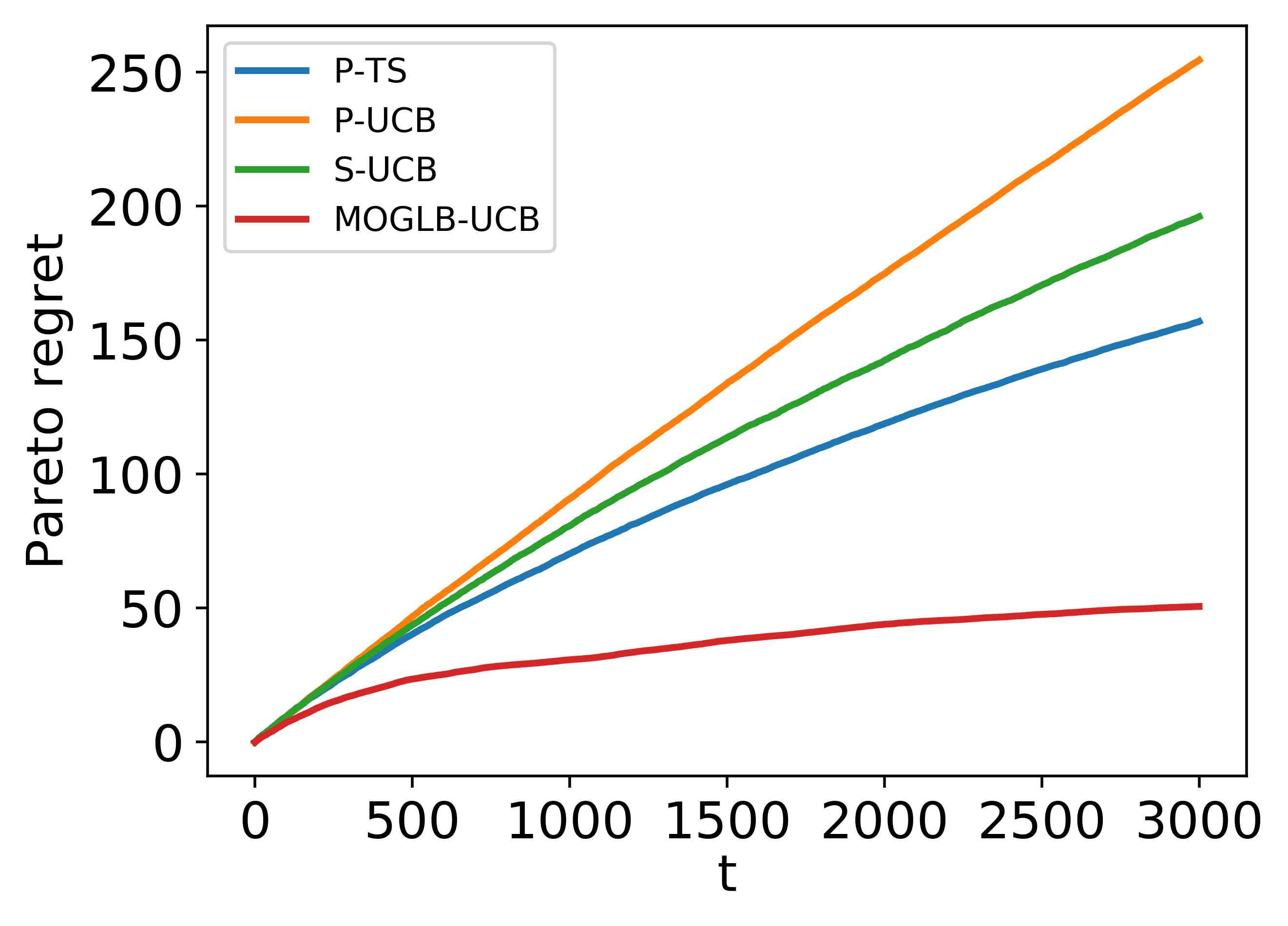
(b) $d=10$

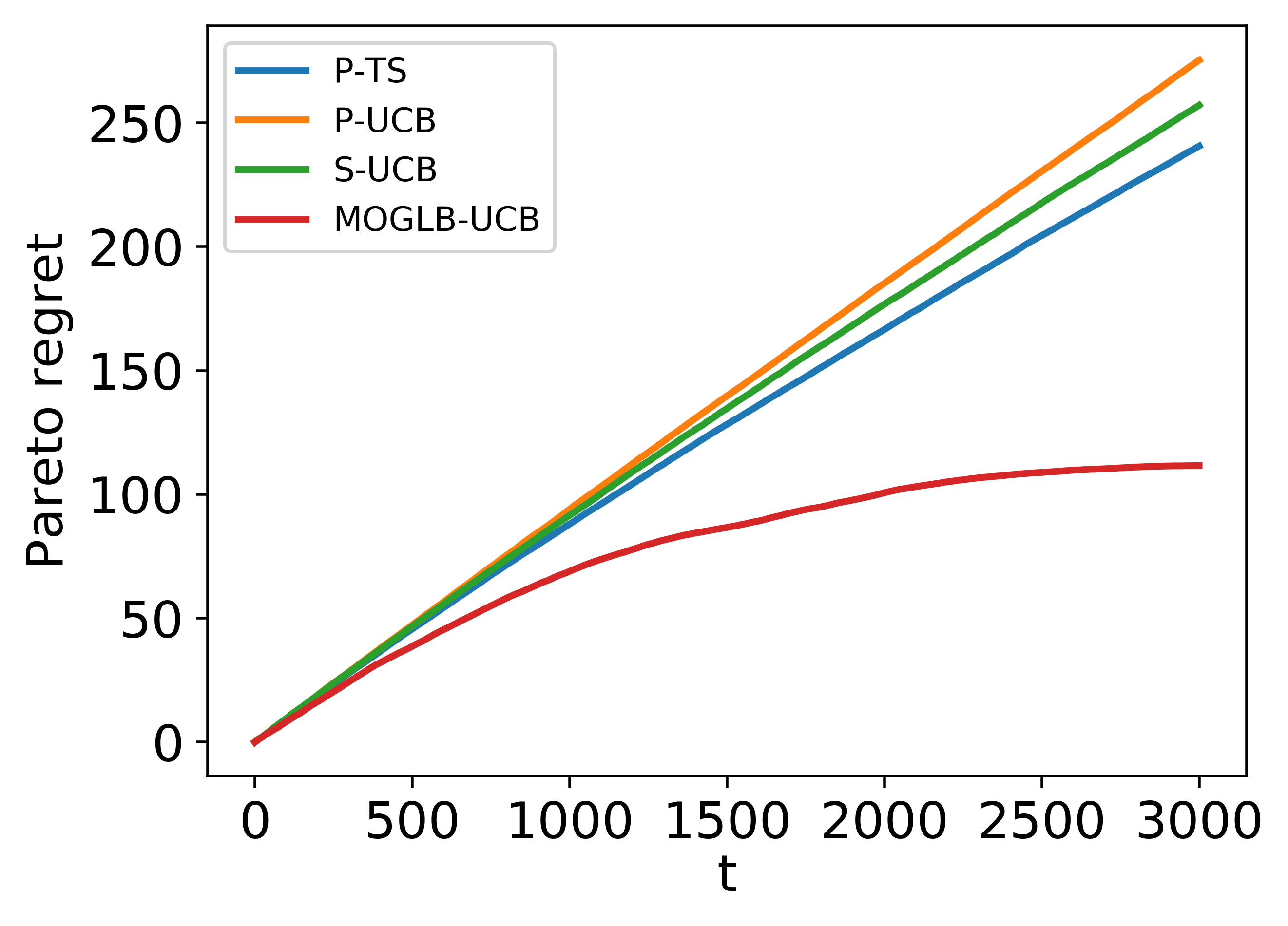
(c) $d=15$

Figure 1: Pareto regret of different methods

5 Experiments

In this section, we conduct numerical experiments to compare our algorithm with the following multi-objective bandits algorithms.

• P-UCB Drugan and Nowe (2013): This is the Pareto UCB algorithm, which compares different arms by the upper confidence bounds of their expected reward vectors and pulls an arm uniformly from the approximate Pareto front.

• S-UCB Drugan and Nowe (2013): This is the scalarized UCB algorithm, which scalarizes the reward vector by assigning weights to each objective and then employs the single objective UCB algorithm Auer et al. (2002a). Throughout the experiments, we assign each objective with equal weight.

• P-TS Yahyaa and Manderick (2015): This is the Pareto Thompson sampling algorithm, which makes use of the Thompson sampling technique to estimate the expected reward for every arm and selects an arm uniformly at random from the estimated Pareto front.

Note that the Pareto contextual zooming algorithm proposed by Turgay et al. Turgay et al. (2018) is not included in the experiments, because one step of this algorithm is finding relevant balls whose specific implementation is lacked in their paper and no experimental results of their algorithm are reported as well.

In our algorithm, there is a parameter $\lambda$. Since its functionality is just to make $Z_{t}$ invertible and our algorithm is insensitive to it, we simply set $\lambda=\max(1,\kappa/2)$. Following common practice in bandits learning Zhang et al. (2016); Jun et al. (2017), we also tune the width of the confidence set $\gamma_{t}$ as $c\log{\frac{\det{(Z_{t})}}{\det{(Z_{1})}}}$, where $c$ is searched within $[1e-3,1]$. We use a synthetic dataset constructed as follows. Let $m=5$ and pick $d$ from $\{5,10,15\}$. For each objective $i\in[m]$, we sample the coefficients $\theta_{i}$ uniformly from the positive part of the unit ball. To control the size of the Pareto front, we generate the arm set comprised of $4d$ arms as follows. We first draw $3d$ arms uniformly from the centered ball whose radius is $0.5$, and then sample $d$ arms uniformly from the centered unit ball. We repeat this process until the size of the Pareto front is not more than $d$.

In each round $t=1,2,\ldots,T$, after the learner submits an arm $x_{t}$, he observes an $m$-dimensional reward vector, each component of which is generated according to the generalized linear model. While the GLM family contains various statistical models, in the experiments we choose two frequently used models namely the probit model and the logit model. Specifically, the first two components of the reward vector are generated by the probit model, and the last three components are generated by the logit model.

Since both the problem and the algorithms involve randomness, we perform $10$ trials up to round $T=3000$ and report average performance of the algorithms. As can be seen from Fig. 1, where the vertical axis represents the cumulative Pareto regret up to round $t$, our algorithm significantly outperforms its competitors in all experiments. This is expected since all these algorithms are designed for multi-armed bandits problem and hence do not utilize the particular structure of the problem considered in this paper, which is explicitly exploited by our algorithm.

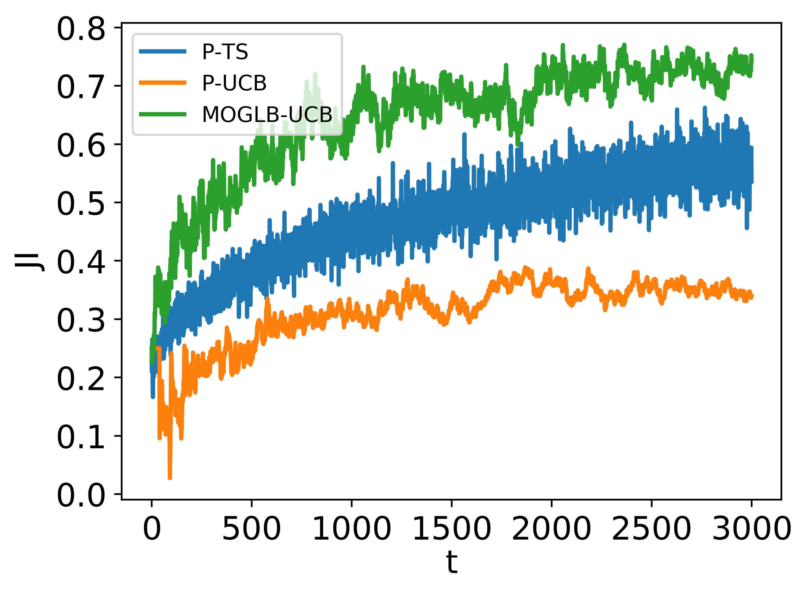
Figure 2: Jaccard index of different methods

Finally, we would like to investigate the issue of fairness. To this end, we examine the approximate Pareto front $\mathcal{O}_{t}$ constructed by the tested algorithms except S-UCB and use Jaccard index (JI) to measure the similarity between $\mathcal{O}_{t}$ and the true Pareto front $\mathcal{O}^{*}$, defined as

$${\rm JI}_{t}\coloneqq\frac{|\mathcal{O}_{t}\cap\mathcal{O}^{*}|}{|\mathcal{O}_{t}\cup\mathcal{O}^{*}|}$$

for which the larger the better.

We plot the curve of ${\rm JI}_{t}$ for each algorithm in Fig. 2, where we set $d=10$. As can be seen, our algorithm finds the true Pareto front much faster than P-UCB and P-TS. Furthermore, the approximate Pareto front constructed by our algorithm is very close to the true Pareto front when $t>1500$. Combining with the result shown in Fig. 1 and the uniform sampling strategy used in Step 3 of Algorithm 1, we observe that our algorithm indeed minimizes the Pareto regret while ensuring fairness.

6 Conclusion and Future Work

In this paper, we propose a novel bandits framework named multi-objective generalized linear bandits, which extends the multi-objective bandits problem to contextual setting under the parameterized realizability assumption. By employing the principle of “optimism in face of uncertainty”, we develop a UCB-type algorithm whose Pareto regret is upper bounded by $\tilde{O}(d\sqrt{T})$, which matches the optimal regret bound for single objective contextual bandits problem.

While we have conducted numerical experiments to show that the proposed algorithm is able to achieve high fairness, it is appealing to provide a theoretical guarantee regarding fairness. We will investigate this in future work.

References

- Abbasi-Yadkori et al. [2011] Yasin Abbasi-Yadkori, Dávid Pál, and Csaba Szepesvári. Improved algorithms for linear stochastic bandits. In Advances in Neural Information Processing Systems 24, pages 2312–2320, 2011.
- Abbasi-Yadkori et al. [2012] Yasin Abbasi-Yadkori, David Pal, and Csaba Szepesvari. Online-to-confidence-set conversions and application to sparse stochastic bandits. In International Conference on Artificial Intelligence and Statistics, pages 1–9, 2012.
- Agarwal et al. [2014] Alekh Agarwal, Daniel Hsu, Satyen Kale, John Langford, Lihong Li, and Robert Schapire. Taming the monster: A fast and simple algorithm for contextual bandits. In International Conference on Machine Learning, pages 1638–1646, 2014.
- Auer et al. [2002a] Peter Auer, Nicolo Cesa-Bianchi, and Paul Fischer. Finite-time analysis of the multiarmed bandit problem. Machine learning, 47(2-3):235–256, 2002.
- Auer et al. [2002b] Peter Auer, Nicolo Cesa-Bianchi, Yoav Freund, and Robert E Schapire. The nonstochastic multiarmed bandit problem. SIAM journal on computing, 32(1):48–77, 2002.
- Auer et al. [2016] Peter Auer, Chao-Kai Chiang, Ronald Ortner, and Madalina Drugan. Pareto front identification from stochastic bandit feedback. In International Conference on Artificial Intelligence and Statistics, pages 939–947, 2016.
- Auer [2002] Peter Auer. Using confidence bounds for exploitation-exploration trade-offs. Journal of Machine Learning Research, 3(Nov):397–422, 2002.
- Bubeck and Cesa-Bianchi [2012] Sébastien Bubeck and Nicolo Cesa-Bianchi. Regret analysis of stochastic and nonstochastic multi-armed bandit problems. Foundations and Trends in Machine Learning, 5(1):1–122, 2012.
- Bubeck et al. [2009] Sébastien Bubeck, Gilles Stoltz, Csaba Szepesvári, and Rémi Munos. Online optimization in -armed bandits. In Advances in Neural Information Processing Systems 22, pages 201–208, 2009.
- Dani et al. [2008] Varsha Dani, Thomas P. Hayes, and Sham M. Kakade. Stochastic linear optimization under bandit feedback. In Conference on Learning Theory, page 355, 2008.
- Drugan and Nowe [2013] MM Drugan and A Nowe. Designing multi-objective multi-armed bandits algorithms: a study. In International Joint Conference on Neural Networks, pages 2352–2359, 2013.
- Drugan and Nowé [2014] Madalina M Drugan and Ann Nowé. Scalarization based pareto optimal set of arms identification algorithms. In International Joint Conference on Neural Networks, pages 2690–2697, 2014.
- Dudik et al. [2011] Miroslav Dudik, Daniel Hsu, Satyen Kale, Nikos Karampatziakis, John Langford, Lev Reyzin, and Tong Zhang. Efficient optimal learning for contextual bandits. In Conference on Uncertainty in Artificial Intelligence, pages 169–178, 2011.
- Filippi et al. [2010] Sarah Filippi, Olivier Cappe, Aurélien Garivier, and Csaba Szepesvári. Parametric bandits: The generalized linear case. In Advances in Neural Information Processing Systems 23, pages 586–594, 2010.
- Hazan et al. [2007] Elad Hazan, Amit Agarwal, and Satyen Kale. Logarithmic regret algorithms for online convex optimization. Machine Learning, 69(2-3):169–192, 2007.
- Jun et al. [2017] Kwang-Sung Jun, Aniruddha Bhargava, Robert Nowak, and Rebecca Willett. Scalable generalized linear bandits: Online computation and hashing. In Advances in Neural Information Processing Systems 30, pages 99–109, 2017.
- Kleinberg et al. [2008] Robert Kleinberg, Aleksandrs Slivkins, and Eli Upfal. Multi-armed bandits in metric spaces. In Proceedings of the 40th Annual ACM Symposium on Theory of Computing, pages 681–690, 2008.
- Langford and Zhang [2008] John Langford and Tong Zhang. The epoch-greedy algorithm for multi-armed bandits with side information. In Advances in Neural Information Processing Systems 21, pages 817–824, 2008.
- Li et al. [2010] Lihong Li, Wei Chu, John Langford, and Robert E Schapire. A contextual-bandit approach to personalized news article recommendation. In International Conference on World Wide Web, pages 661–670, 2010.
- Lu et al. [2010] Tyler Lu, Dávid Pál, and Martin Pál. Contextual multi-armed bandits. In International Conference on Artificial Intelligence and Statistics, pages 485–492, 2010.
- Lu et al. [2019] Shiyin Lu, Guanghui Wang, Yao Hu, and Lijun Zhang. Optimal algorithms for Lipschitz bandits with heavy-tailed rewards. In Proceedings of the 36th International Conference on Machine Learning, pages 4154–4163, 2019.
- Nelder and Wedderburn [1972] J. A. Nelder and R. W. M. Wedderburn. Generalized linear models. Journal of the Royal Statistical Society, Series A, General, 135:370–384, 1972.
- Rodriguez et al. [2012] Mario Rodriguez, Christian Posse, and Ethan Zhang. Multiple objective optimization in recommender systems. In Proceedings of the sixth ACM conference on Recommender systems, pages 11–18. ACM, 2012.
- Slivkins [2014] Aleksandrs Slivkins. Contextual bandits with similarity information. Journal of Machine Learning Research, 15(1):2533–2568, 2014.
- Turgay et al. [2018] Eralp Turgay, Doruk Oner, and Cem Tekin. Multi-objective contextual bandit problem with similarity information. In International Conference on Artificial Intelligence and Statistics, pages 1673–1681, 2018.
- Yahyaa and Manderick [2015] Saba Yahyaa and Bernard Manderick. Thompson sampling for multi-objective multi-armed bandits problem. In European Symposium on Artificial Neural Networks, pages 47–52, 2015.
- Zhang et al. [2016] Lijun Zhang, Tianbao Yang, Rong Jin, Yichi Xiao, and Zhi-hua Zhou. Online stochastic linear optimization under one-bit feedback. In International Conference on Machine Learning, pages 392–401, 2016.