Fast Reciprocal Collision Avoidance Under Measurement Uncertainty

Abstract

We present a fully distributed collision avoidance algorithm based on convex optimization for a team of mobile robots. This method addresses the practical case in which agents sense each other via measurements from noisy on-board sensors with no inter-agent communication. Under some mild conditions, we provide guarantees on mutual collision avoidance for a broad class of policies including the one presented. Additionally, we provide numerical examples of computational performance and show that, in both 2D and 3D simulations, all agents avoid each other and reach their desired goals in spite of their uncertainty about the locations of other agents.

1 Introduction

Reliable collision avoidance is quickly becoming a mainstay requirement of any scalable mobile robotics system. As robots continue to be deployed around humans, assurances of safety become more critical, especially in high traffic areas such as factory floors and hospital corridors. We present an on-line, distributed collision avoidance algorithm based on convex optimization that generates robot controls to evade moving obstacles sensed using noisy on-board sensors. We also show that a general class of controllers, including the one presented, guarantees mutual collision avoidance, provided that all robots involved use this policy.

We allow for each robot to have its own estimate of the relative positions of other robots, which may be inconsistent with the other robots’ estimates. To conservatively manage uncertainty in this model, we assume that each robot keeps an uncertainty set (e.g., unions and intersections of ellipsoids) that contain other robots’ possible locations. We assume each robot knows its own position exactly and updates its estimates of the other robots via noisy on-board sensors such as a camera or LIDAR.

The policy is distributed in the sense that each robot only requires an estimate of the relative positions of the other robots. In other words, robots do not need to communicate their position or explicitly coordinate actions with nearby robots. Each agent then uses these position estimates to find a safe-reachable set which is characterized by a generalized Voronoi partition. Our algorithm computes a projection onto this set, which we show reduces to an efficiently solvable convex optimization problem. Our method is amenable to fast convex optimization solvers, resulting in computations times of approximately 18 ms for 100 obstacles in 3D, including setup and solution time. Furthermore, we prove that if each agent uses this policy then mutual collision avoidance is guaranteed.

This paper is organized as follows. The remainder of this section discusses related work. Section 2 formulates the mutual avoidance problem and gives the necessary mathematical background on generalized Voronoi partitioning. Section 3 describes the collision-avoidance algorithm and provides a collision avoidance guarantee. Section 4 formalizes the projection problem and describes the resulting convex optimization for ellipsoidal uncertainties in detail. Finally, section 5 shows our method’s computational performance. Additionally, we show in 2D and 3D simulations that all agents avoid each other and navigate to their goal locations despite their positional uncertainty of other agents.

1.1 Related Work

The most closely related methods for fully distributed collision avoidance in the literature are the velocity obstacle (VO) methods, which can be used for a variety of collision avoidance strategies. These methods work by extrapolating the next position of an obstacle using its current velocity. One of the most common tools used for mutual collision avoidance is the Reciprocal Velocity Obstacles (RVO) [VdBLM08, VdBGLM11, VdBGS⁺16] method in which each agent solves a linear program to find its next step. The Buffered Voronoi Cell (BVC) [ZWBS17] method provides similar avoidance guarantees but does not require the ego agent to know other agents’ velocities, which can be difficult to estimate accurately. The BVC algorithm opts instead for defining a given distance margin to compute safe paths. BVC methods have been coupled with other decentralized path planing tools [ŞHA19] in order to successfully navigate more cluttered environments, but require that the other agents’ positions are known exactly.

While both VO and BVC methods scale very well to many (more than 100) agents, they also require perfect state information of other agents’ positions (BVC), or positions and velocities (RVO). In many practical cases, high accuracy state information, especially velocity, may not be accessible as agents are estimating the position of the same objects they are trying to avoid. Extensions to VO that account for uncertainty have been studied under bounded [CHTM12] and unbounded [GSK⁺17] localization uncertainties by utilizing chance constraints. While these have been extended to decentralized methods [ZA19], they assume constant velocity of the obstacles at plan time. Combined Voronoi partitioning and estimation methods have been studied for mult-agent path planing tasks [BCH14], but still require communication to build an estimate via consensus. In contrast, our method does not require any communication or velocity state information, nor does it require the true position of the other agents. Instead, the algorithm uses only an estimate of the current position of the nearby agents and their reachable set within some time horizon.

Our algorithm takes a nominal desired trajectory or goal point (which can come from any source, much like [VdBLM08, ZWBS17]), and returns a safe next step for an agent to take while accounting for both the uncertainty and the physical extent of the other agents in the vicinity. The focus of this work is on fast, on-board refinement rather than total path planning. More specifically, while the algorithm presented could be used to reach a far away goal point, it is likely more useful as a small-to-medium scale planner for reaching waypoints in a larger, centrally or locally planned, trajectory.

Similarly, single agent path planners such as A* or rapidly-exploring random trees (RRT) can be applied to the multi-agent case, but the solution times grow rapidly due to the exploding size of the joint state space. For example, graph-search methods can be partially decoupled [WC11] to better scale for larger multi-agent systems, but can explore the entire joint state-space in the worst case. Fast Marching Tree (FMT) methods [JSCP15] are similar to RRTs in that they dynamically build a graph via sampling. But, while FMT methods have better performance in higher dimensional systems, they still require the paths to be centrally calculated. Using barrier functions [MJWP16], A* can also be used in dense environments for decentralized multi-agent planning, but require the true position of all the other agents. On the other hand, while all of these methods require global knowledge and large searches over a discrete set, they can be used as waypoint generators that feed into our method—for use, e.g., in cluttered environments.

Optimization methods that use sequential convex programming (SCP) [SHL⁺13, ASD12, MCH14] have also been studied for multi-agent path planning; however, these algorithms are still centralized and may exhibit slow convergence, making them unreliable for on-line planning. For some systems, these methods can be partially decoupled [CCH15], reducing computation time at the cost of potentially returning infeasible paths. Our method, in comparison, is fully decentralized and produces an efficient convex program for each agent. The solution of this program is a safe waypoint for the agent, which, unlike SCP methods, requires no further refinment.

2 Problem Formulation

Consider a group of $N$ dynamic agents. Let $x_{i}(t)\in{\mbox{\bf R}}^{n}$ be the position of agent $i$ (also referred to as the “ego agent”) for $i=1,\dots,{N}$ at time $t=1,\dots,{T}$, where each agent satisfies single integrator dynamics,

$$x_{i}(t+1)=x_{i}(t)+u_{i}(t),~{}~{}i=1,\dots,{N},~{}~{}t=1,\dots,{T},$$ (1)

with control $u_{i}(t)\in{\mbox{\bf R}}^{n}$ and $\left\|{u_{i}(t)}\right\|_{2}\leq u^{\mathrm{max}}$. In addition, every agent $i$ will maintain a set-based estimate of the location of every other agent $j\neq i$ as a set $\mathcal{E}^{j}_{i}(t)$, such that

$$x_{j}(t)\in\mathcal{E}^{j}_{i}(t),~{}~{}i=1,\dots,{N},~{}~{}t=1,\dots,{T}.$$ (2)

In other words, the true position of agent $j$ at time $t$ must always be inside the noisy estimate $\mathcal{E}^{j}_{i}(t)$ maintained by agent $i$. In practice, this set can be obtained from a high probability confidence ellipsoid of a Bayesian filter or from a set-membership filter [BR71]. We do not restrict the size of this uncertainty region, though we note that large uncertainties will restrict an agent’s possible actions.

Let the safe-reachable set $S_{i}(t)$ be the generalized Voronoi cell [Wat81, HZZ⁺12, SS19] generated between agent $i$’s current position, $x_{i}(t)$, and the set of estimates, $\mathcal{E}^{j}_{i}$, that agent $i$ has of every agent $j$ at time $t$. That is,

$$S_{i}(t)=\left\{z~{}\middle|~{}\left\|{z-x_{i}(t)}\right\|_{2}\leq\|z-\mathcal{E}^{j}_{i}(t)\|_{2}~{}~{}\forall j=1,\dots,{N},~{}j\neq i\right\}$$ (3)

where $\|z-\mathcal{E}^{j}_{i}(t)\|_{2}$ is the distance-to-set metric $\|z-\mathcal{E}^{j}_{i}(t)\|_{2}=\inf_{y\in\mathcal{E}^{j}_{i}(t)}\left\|{z-y}\right\|_{2}$.

More explicitly, $S_{i}(t)$ is the set of points which lie closer to agent $i$ than to any possible position of agent $j$ within its uncertainty set $\mathcal{E}^{j}_{i}$. This has a natural interpretation in the case where all agents share the same single-integrator dynamics (though this condition is not necessary for the algorithm, in general): $S_{i}(t)$ is the set of all points which agent $i$ is guaranteed to reach from its current position before any other agent. We emphasize that since each agent will often maintain different estimates of the positions of other agents, the sets $S_{i}(t)$ generally do not form a partition of ${\mbox{\bf R}}^{n}$, as the union $\cup_{i}S_{i}(t)$ does not equal the entire space. Figure 1 shows the generalized Voronoi cell boundaries in an example simulation: each agent is shown with the estimates it has of other agents, along with the agent’s goal position and projected goal position.

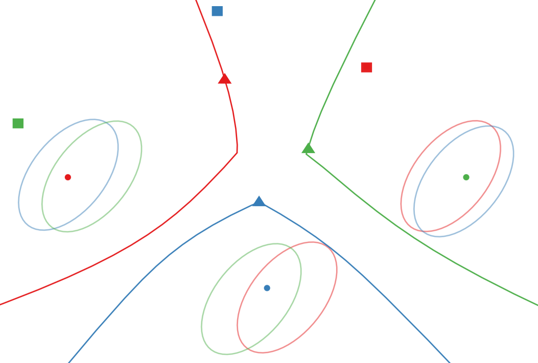
Figure 1: Generalized Voronoi cells of each (blue, red, green) agent’s position (circle) with goal point (square) and safe projected goal point (triangle). Each agent uses an ellipsoidal estimate (colored ellipses) of each other agent’s position to generate its own cell.

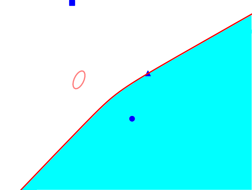
Figure 2: Projection (blue triangle) of a goal point (blue square) onto a generalized Voronoi region (cyan region). The boundary (red curve) is equidistant from the agent’s position (blue point) and the closest point inside the ellipsoidal estimate of the obstacle (red ellipse).

We also note that $S_{i}(t)$ is a relatively conservative estimate of the set of collision-free points. Let

$$\mathcal{E}_{i}(t)=\bigcup_{\begin{subarray}{c}j=1\\ j\neq i\end{subarray}}^{N}\mathcal{E}^{j}_{i}(t),$$

that is, $\mathcal{E}_{i}(t)$ is the set of all points which could potentially include another agent—from the perspective of agent $i$—then the safe-reachable set satisfies

$$S_{i}(t)\subseteq{\mbox{\bf R}}^{n}\setminus\mathcal{E}_{i}(t).$$

Additionally, we note that each set $S_{i}(t)$ is the intersection of an infinite number of half-spaces since (3) can be rewritten as

$$S_{i}(t)=\bigcap_{y\in\mathcal{E}_{i}(t)}\left\{z~{}\middle|~{}\left\|{z-x_{i}}\right\|_{2}\leq\left\|{z-y}\right\|_{2}\right\},$$ (4)

which implies that $S_{i}(t)$ is a convex set [BV04, §2.3.1]. This means that a projection of an arbitrary point (such as a goal destination or way-point) onto this set can be formulated as a (potentially infinitely large) convex optimization problem. In the next section, we describe an algorithm which uses these projections and then prove collision-free guarantees for this algorithm, while in the following section, we show how these projections can be efficiently computed.

Normally, uncertainties are defined for points in space (i.e., the center of a robot in ${\mbox{\bf R}}^{3}$); however, without physical extent, collision is a measure zero event. To guarantee collision avoidance, we must account for the uncertainty as well as the physical size of the other agents. Assuming that the robot’s physical extent can be represented by an ellipsoid, we can combine the physical size ellipsoid with the uncertainty ellipsoid such that their Minkowski sum is contained inside another bounding ellipsoid $\bar{\mathcal{E}}$. In particular, we seek a $\bar{\mathcal{E}}\supseteq\mathcal{E}_{\mathrm{estimate}}\oplus\mathcal{E}_{\mathrm{size}}$. We can find a small ellipsoid which satisfies this propety efficiently (in fact, analytically) by solving a minimum trace optimization problem, the details can be found in [LZW16]. Additionally, using ellipsoidal margins allows us to potentially account for more complicated effects that could not be reasonably represented by spherical margins. For example, [PHAS17] uses ellipsoids elongated in the $z$-axis to generate keepout zones above and below quadrotors which account for the downwash effect of the propellers.

3 Collision Avoidance

We present an algorithm which uses the projections described in section 2 to reach a given goal. We then present a general proof of collision avoidance guarantees for a class of algorithms including the one presented in [ZWBS17] and Algorithm 1 (below), along with its natural extensions.

3.1 General Algorithm

To simplify notation, let $R_{i}(t)$ be the reachable set of positions of each agent $i$ at time $t$. We note that, in our case, $R_{i}(t)$ is the intersection of the closed $\ell_{2}$-ball with radius $u^{\mathrm{max}}$ and the generalized Voronoi cell of agent $i$ at time $t$. We also note that this is a compact set which always contains $0$ if it is not empty.

Let $\mathcal{E}_{i}^{j}(t)$ be the uncertainty ellipsoid with nonzero volume that agent $i$ has of agent $j\neq i$ at time $t$ and let $P_{i}(x_{i},\mathcal{E}_{i},t)$ be the projection of agent $i$’s goal into the intersection of its generalized Voronoi cell and its reachable set at time $t$. As a technical requirement, we will require that agent $j$’s true position lies in the interior of $\mathcal{E}_{i}^{j}(t)$. Since this projection can fail (e.g., when agent $i$’s uncertainty of agent $j$’s position is large enough to include the position of agent $i$), we allow the projection function to return either a point in ${\mbox{\bf R}}^{n}$, or a symbol, $\neg$, which indicates that the projection failed—i.e., there is no safe point to move to.

Algorithm 1 General projection algorithm

  $i\leftarrow$ current agent.

  $x_{i}(1)\leftarrow$ initial position of agent $i$.

  for $t=1,\dots,T$ do

     $q\leftarrow P_{i}(x_{i},\mathcal{E}_{i},t)$

     if $q=\neg$ then

        $x_{i}(t+1)\leftarrow x_{i}(t)$

     else if $q\neq\neg$ then

        $x_{i}(t+1)\leftarrow q$

     end if

  end for

Algorithm 1 states that, if the projection fails, the agent does not move from its current position; otherwise, the agent moves towards the next projection.

Theorem 1.

Algorithm 1 is collision free, assuming all agents start from a collision free configuration.

Proof.

First, we note the following properties of the projection function defined above. If the function yields a point in ${\mbox{\bf R}}^{n}$ (and not $\neg$) then the following statements are satisfied,

$$P_{i}(x_{i},\mathcal{E}_{i},t) \in x_{i}(t)+R_{i}(t),~{}~{}~{}t=1,\dots,T$$ (5)

$$P_{i}(x_{i},\mathcal{E}_{i},t) \not\in x_{j}(t)+R_{j}(t),~{}~{}~{}t=1,\dots,T,~{}~{}j=1,\dots,N,~{}~{}j\neq i,$$

where the sum of a vector $v\in{\mbox{\bf R}}^{n}$ and a set $M\subseteq{\mbox{\bf R}}^{n}$ is defined as $v+M=\{v+w\mid w\in M\}$. In other words, condition (5) requires that the projection, if it returns a point, must (a) return a point which is in the agent’s reachable set, and (b) cannot return a point which could lie in region of another agent’s reachable set, since agent $i$ does not know where agent $j$ is headed.

The first statement (a) comes from the fact that, by definition, the projection function gives a point in the intersection of the reachable set and the generalized Voronoi cell. The second (b) comes from the fact that the set which we project into contains only the points which are reachable by agent $i$ before they are by agent $j$, and agent $j$ maintains an uncertainty ellipsoid of agent $i$’s position which includes agent $i$’s true position. This implies that the reachable set of agent $j$ at time $t$ cannot include the projection of agent $i$ at time $t$.

Now, assume that all agents start a positive distance apart at time $t=1$ and consider any two agents $i\neq j$. Recall that our projection function $P_{i}(x_{i},\mathcal{E}_{i},t)$ returns a point or returns $\neg$. Suppose that a point is returned, then, by definition of algorithm 1 and by (5), we know that

$$x_{i}(t+1)=P_{i}(x_{i},\mathcal{E}_{i},t)\not\in x_{j}(t)+R_{j},$$

so $x_{i}(t+1)$ must be a positive distance from $x_{j}(t)+R_{j}(t)$, by compactness of $R_{j}(t)$. Since, by definition, $x_{j}(t)+R_{j}(t)$ contains the point $x_{j}(t+1)$, then $x_{i}(t+1)$ is always a positive distance away from $x_{j}(t+1)$.

Now, assume that $P_{i}(x_{i},\mathcal{E}_{i},t)$ returns $\neg$, then, for the other agent, $P_{j}(x_{j},\mathcal{E}_{j},t)$ either returns $\neg$ (in which case no collision happens, since neither agent has moved, by definition of algorithm 1) or $P_{j}$ returns a point which satisfies

$$x_{j}(t+1)=P_{j}(x_{j},\mathcal{E}_{j},t)\not\in x_{i}(t)+R_{i}(t).$$

But, since agent $i$ has not moved, $x_{i}(t+1)=x_{i}(t)\in x_{i}(t)+R_{i}(t)$ (since $0\in R_{i}(t)$, by definition), so $x_{j}(t+1)$ is a positive distance away from $x_{i}(t+1)$, again by compactness of $R_{i}(t)$.

Since this is true for any two agents, then all agents stay a positive distance apart from each other for each time $t=1,\dots,T$, and no collision happens. ∎

3.2 Generalizations and discussion

While the proof above is presented only in the context of algorithm 1 with the projection function and reachable sets specified in §2, the proof is almost immediately generalizable to many other projection functions and reachable sets. We present a few of these generalizations below.

Proof requirements.

In the proof of theorem 1, we only used the following three facts: (a) the projection function satisfies (5), (b) that $R_{i}(t)$ was compact for each agent $i$ at each time $t$, and (c) that 0 is in the reachable set ($0\in R_{i}(t)$). This means that any set of agents and projection functions that satisfy the above conditions are immediately guaranteed to be collision free, if they use algorithm 1. There are many such projection functions, for example the trivial function (which always returns $\neg$) and functions which are potentially very complicated and depend on the histories of the uncertainties, but all cases guarantee collision avoidance so long as these conditions are satisfied.

Minimum distance.

The minimum distance between agents depends on the aggressiveness of the projection function—in the sense that the proof above only guarantees a non-zero (but arbitrarily small) separation. We can give slightly better bounds by under-projecting to ensure that, for every $i\neq j$ and time $t$,

$$\|P_{i}(x_{i},\mathcal{E}_{i},t)-(x_{j}(t)+R_{j}(t))\|_{2}\geq\varepsilon>0.$$ (6)

This guarantees that every pair of agents will have a separation of at least $\varepsilon$.

It is sometimes easy to generate the under-projection condition in (6). For example, this is possible in the case where $R_{j}(t)$ is a convex set and $\{P_{j}\}$ is any set of valid projection functions. To generate this, we choose the $q$ of algorithm 1 to be a convex combination of the current position and the projected position which satisfies the inequality above. This ensures that every pair of agents is at least $\varepsilon$-separated—assuming all agents start with at least $\varepsilon$ separation at time $t=1$—for all $t=1,\dots,T$.

Uncertainties.

The sets $\mathcal{E}_{i}^{j}(t)$ for $t=1,\dots,T$ and $j=1,\dots,N$ with $j\neq i$ only play a role as the arguments to $P_{i}$, but there is no requirement that these measurements be accurate or even bounded in any sense. It is possible for one agent to temporarily have large uncertainty about the positions of all other agents (e.g., in the case of GPS loss) before gaining a more accurate measurement and continuing to its objective. Of course, the usefulness of the projection function will heavily depend on the quality of these projections, but we are guaranteed to be collision free at every point in time, independent of these assumptions, so long as condition (5) is satisfied.

Relaxing the reachability condition.

In the proof of theorem 1 we assume that the current position is always a reachable state for agent $i$ (i.e., that $0\in R_{i}(t)$). While this is the case in single-integrator dynamics, for example, it is not the case in general. It is possible to weaken this assumption slightly by ensuring that the agent can stop within some $\varepsilon$-ball, such that some point in $x_{i}(t)+\varepsilon B$ is always reachable (where $\varepsilon>0$ and $B=\{x\in{\mbox{\bf R}}^{n}\mid\left\|{x}\right\|_{2}\leq 1\}$) from state $x_{i}(t)$, but the assumptions on the projection functions, $P_{i}$, must be strengthened considerably from the general ones given in condition (5).

Asymmetric dynamics.

It is rarely the case that the dynamics of the agents in question are single-integrator dynamics with the same maximal input for all agents, as we assumed at the beginning of this proof. In the case that the dynamics are asymmetric among agents, we can guarantee condition (5) with the projections presented in this section by simply expanding the uncertainty ellipsoid by a margin which includes the reachability of the other agents. That is, we can replace the uncertainty ellipsoid that agent $i$ has of agent $j$, originally given by $\mathcal{E}_{i}^{j}(t)$ at time $t$ with $\mathcal{E}_{i}^{j}(t)\oplus R_{j}(t)$ (or any other outer envelope of this set). Using this new uncertainty to generate a safe Voronoi region and using its corresponding projection, as given in §2, is then guaranteed to be collision free.

4 Projecting onto Generalized Voronoi Cells

In this section, we describe a solution to the problem of efficiently projecting a point into a generalized Voronoi region.

First, we construct a program which is equivalent to finding a projection into a convex set of the form (4), but may not be easy to solve as its constraint is not representable in any standard form. We then use Lagrange duality to construct a convex constraint that is at least as strict as the original and use strong duality to show that this constraint is equivalent to the original problem. Finally, we provide a conic problem for the case of ellipsoid generated Voronoi regions with the constraint explicitly parametrized by the ellipsoid parameters $(\mu,\Sigma)$. We also show that, for the ellipsoidal case, the constraint is represented by a sum of quadratic-over-linear terms, implying that the convex program is a second order cone program (SOCP) and can therefore be solved quickly by embedded solvers.

4.1 Problem Statement

As in [ZWBS17], in order to execute the collision-avoidance strategy, each agent must project its goal point onto its safe-reachable set as defined in (4). This problem is always convex since the Voronoi region is generated by an (arbitrary) intersection of hyperplanes [BV04, §2.3.1], which always results in a convex set.

Consider the case in which the Voronoi cell is generated by a point $x$ and a single convex set, $\mathcal{E}$, defined by

$$\mathcal{E}=\{y~{}|~{}f(y)\leq 0\},$$

where $f:{\mbox{\bf R}}^{n}\to{\mbox{\bf R}}^{m}$ is a convex function and the inequality is taken elementwise. This allows us to write the problem as finding a projection point $x$ which solves

$$\underset{x}{\text{minimize}} \left\|{x-x^{\mathrm{g}}}\right\|_{2}^{2}$$ (7)

subject to $$x\in V(x^{\mathrm{c}},\mathcal{E})$$

where $x^{\mathrm{c}}$ is the current position of the agent, $x^{\mathrm{g}}$ is the goal, and $V(x^{\mathrm{c}},\mathcal{E})$ is the agent’s generalized Voronoi region,

$$V(x^{\mathrm{c}},\mathcal{E})=\{z\mid\left\|{z-x^{\mathrm{c}}}\right\|_{2}\leq\inf_{y\in\mathcal{E}}\left\|{z-y}\right\|_{2}\}.$$

For some special cases of $\mathcal{E}$, such as a circle or sphere, the constraint’s infimum can be found analytically. However, this may not be possible for arbitrary sets. For example, in the case where $\mathcal{E}$ is an ellipsoid, no analytical distance function has been found [UG18].

Using the definitions of $\mathcal{E}$ and $V(x^{\mathrm{c}},\mathcal{E})$, we can write (7) as

$$\underset{x}{\text{minimize}} \left\|{x-x^{\mathrm{g}}}\right\|_{2}^{2}$$ (8)

subject to $$\left\|{x^{\mathrm{c}}}\right\|_{2}^{2}-2x^{T}x^{\mathrm{c}}\leq\inf_{f(y)\leq 0}\left(\left\|{y}\right\|_{2}^{2}-2x^{T}y\right).$$

This is the problem formulation we will use throughout. Figure 2 gives an illustration of the projection problem.

4.2 Lagrange Duality

At the moment, it is not obvious how to represent the the constraint given in problem (8) in a standard or easy-to-solve form.

If we can find a lower bound to the right hand side of the constraint in problem (8) which makes the resulting problem easy to solve, then we can find a feasible (i.e., safe) point, $x$, which may not be optimal. More concretely, suppose we have a function $\hat{g}$ which satisfies, for every $x$,

$$\hat{g}(x)\leq\inf_{f(y)\leq 0}\left(\left\|{y}\right\|_{2}^{2}-2x^{T}y\right),$$

then any $x$ which satisfies

$$\left\|{x^{\mathrm{c}}}\right\|_{2}^{2}-2x^{T}x^{\mathrm{c}}\leq\hat{g}(x),$$

also satisfies

$$\left\|{x^{\mathrm{c}}}\right\|_{2}^{2}-2x^{T}x^{\mathrm{c}}\leq\inf_{f(y)\leq 0}\left(\left\|{y}\right\|_{2}^{2}-2x^{T}y\right),$$

making $x$ a feasible point for problem (8). One standard way of forming such a lower bound is via Lagrange duality [BV04, §5.1]. The Lagrangian of the infimum in (8)

$$\mathcal{L}(y,x,\lambda)=\left\|{y}\right\|_{2}^{2}-2x^{T}y+\lambda^{T}f(y),$$

with $\lambda\in{\mbox{\bf R}}^{m}$ and $\lambda\geq 0$. This gives us the Lagrange dual function

$$g(x,\lambda)=\inf_{y}\mathcal{L}(y,x,\lambda)=\inf_{y}\left(\left\|{y}\right\|_{2}^{2}-2x^{T}y+\lambda^{T}f(y)\right).$$ (9)

By weak duality [BV04, §5.1.3], for every $\lambda\geq 0$ and each $x$,

$$g(x,\lambda)\leq\inf_{f(y)\leq 0}\left(\left\|{y}\right\|_{2}^{2}-2x^{T}y\right),$$

as required.

Additionally, since the dual function $g$ is jointly concave in both $\lambda$ and $x$, the resulting inequality constraint is convex,

$$\left\|{x^{\mathrm{c}}}\right\|_{2}^{2}-2x^{T}x^{\mathrm{c}}\leq g(x,\lambda).$$

Strong duality.

Due to the lower bound property of $g$, the optimization problem,

$$\underset{x,\ \lambda}{\text{minimize}} \left\|{x-x^{\mathrm{g}}}\right\|_{2}^{2}$$ (10)

subject to $$\left\|{x^{\mathrm{c}}}\right\|_{2}^{2}-2x^{T}x^{\mathrm{c}}\leq g(x,\lambda)$$

$$\lambda\geq 0,$$

is potentially more restrictive than the original and is thus an upper bound on the optimal objective of problem (8). Due to strong duality holding in almost all cases of interest (i.e., all cases where the set $\mathcal{E}$ has nonempty interior), we will see that problems (10) and (8) are equivalent which implies that every optimal solution to problem (10) is an optimal solution to problem (8); in other words, the relaxation provided is tight.

In particular, Slater’s condition holds for any convex set $\mathcal{E}$ with non-empty interior (in three dimensions, this would be any convex set with nonzero volume). Since Slater’s condition implies strong duality [BV04, §5.3.2], then for each $x$, there exists some $\lambda^{\star}\geq 0$ such that

$$g(x,\lambda^{\star})=\inf_{f(y)\leq 0}\left(\left\|{y}\right\|_{2}^{2}-2x^{T}y\right),$$

which means that a solution to problem (10) is always a solution to problem (8).

Given an arbitrary convex function $f$, it is unclear if the associated function $g$ defined by (9) has an analytic form or is even easy to evaluate. In the following section, we derive an analytic form for $g$ in the case that $\mathcal{E}$ is an ellipsoid. In the appendix, we also derive an analytic form for $g$ for polyhedral sets. We also show that it is possible to construct more complicated sets from the union and intersection of these ellipsoidal and polyhedral ‘atoms’ allowing the user to specify complicated, non-convex sets as the uncertainty regions of other agents or obstacles.

4.3 Constraints for Regions Generated by Ellipsoids

If the set $\mathcal{E}$ is specified by a convex quadratic constraint, as in the case of ellipsoids, then the set $\mathcal{E}$ can be written as,

$$\mathcal{E} =\{y~{}|~{}f(y)\leq 0\}=\{y~{}|~{}(y-\mu)^{T}\Sigma^{-1}(y-\mu)\leq 1\}$$

with $\mu\in{\mbox{\bf R}}^{n}$ and $\Sigma\in{\mbox{\bf S}}^{n}_{++}$, the positive definite matrix cone, representing the center and shape of the uncertainty, respectively. Note that the minimum of the convex quadratic,

$$y^{T}Ay-2b^{T}y,$$

with $A$ positive definite is given by

$$\inf_{y}\left(y^{T}Ay-2b^{T}y\right)=-b^{T}A^{-1}b.$$

Here, $y^{*}=A^{-1}b$, is found by setting the gradient to zero—this is necessary and sufficient by convexity and differentiability. The dual function is then,

$$g(x,\lambda) =\inf_{y}\left(\left\|{y}\right\|_{2}^{2}-2x^{T}y+\lambda((y-\mu)^{T}\Sigma^{-1}(y-\mu)-1)\right)$$

$$=\inf_{y}\left(y^{T}(\lambda\Sigma^{-1}+I)y-2(x+\lambda\Sigma^{-1}\mu)^{T}y+\lambda\left(\mu^{T}\Sigma^{-1}\mu-1\right)\right)$$

$$=-(x+\lambda\Sigma^{-1}\mu)^{T}(\lambda\Sigma^{-1}+I)^{-1}(x+\lambda\Sigma^{-1}\mu)+\lambda(\mu^{T}\Sigma^{-1}\mu-1).$$

Though the function $g$ can immediately be written in standard semidefinite program (SDP) form via the Schur complement, it is possible to convert it into a second-order cone constraint form, which is usually more amenable to embedded solvers (e.g., ECOS [DCB13]).

First, since $\Sigma$ is positive definite, it has an eigendecomposition $\Sigma=UDU^{T}$, where $U\in{\mbox{\bf R}}^{n\times n}$ is an orthogonal matrix that satisfies $UU^{T}=U^{T}U=I$ and $D\in{\mbox{\bf R}}^{n\times n}$ is a diagonal matrix with positive entries. Using the fact that $\Sigma^{-1}=UD^{-1}U^{T}$, we can write

$$(\lambda\Sigma^{-1}+I)^{-1}=(\lambda UD^{-1}U^{T}+UU^{T})^{-1}=U(\lambda D^{-1}+I)^{-1}U^{T},$$

which gives,

$$g(x,\lambda) =-(U^{T}(x+\lambda\tilde{\mu}))^{T}(D^{-1}+\lambda I)^{-1}(U^{T}(x+\lambda\tilde{\mu}))+\lambda(\tilde{\mu}^{T}\Sigma\tilde{\mu}-1)$$ (11)

$$=-\sum_{i=1}^{n}\frac{(u_{i}^{T}x+\lambda u_{i}^{T}\tilde{\mu})^{2}}{D_{ii}^{-1}+\lambda}+\lambda(\tilde{\mu}^{T}\Sigma\tilde{\mu}-1),$$

where $\tilde{\mu}=\Sigma^{-1}\mu$ and $u_{i}$ is the $i$th column of $U$. After substituting (11) into (8) we obtain the following optimization problem,

$$\underset{x,\ \lambda}{\text{minimize}} \left\|{x-x^{\mathrm{g}}}\right\|_{2}^{2}$$ (12)

subject to $$\left\|{x^{\mathrm{c}}}\right\|_{2}^{2}-2x^{T}x^{\mathrm{c}}+\sum_{i=1}^{n}\frac{(u_{i}^{T}x+\lambda u_{i}^{T}\tilde{\mu})^{2}}{D_{ii}^{-1}+\lambda}\leq\lambda(\tilde{\mu}^{T}\Sigma\tilde{\mu}-1)$$

$$\lambda\geq 0,$$

where $\Sigma$ and $\tilde{\mu}=\Sigma^{-1}\mu$ are given by the uncertainty of the other agent’s position, and $x^{\mathrm{g}}$ and $x^{\mathrm{c}}$ are known by the ego agent (i.e., the agent solving the optimization problem).

As there is a standard approach for converting the sum of $n$ quadratic-over-linear terms into $n$ second-order cone (SOC) constraints (e.g., see [LVBL98]) and an affine constraint, this formulation can then be used directly with embedded SOCP solvers. It can also be automatically converted to an SOCP by modeling languages such as CVXPY [AVDB18].

5 Simulation Results

5.1 Projection Implementation

To get an accurate estimate of the speed of the projection algorithm, the optimization problem outlined in (12) was implemented in the Julia language [BEKS17] using the JuMP mathematical programming language [DHL17] and solved using ECOS [DCB13]. 285 instances of the problem were generated with 100 randomly generated ellipsoids in ${\mbox{\bf R}}^{3}$. Timing and performance results for generating and solving the corresponding convex program can be found in table 1. Figure 3 shows how the performance scales as the number of other agents increases. All times reported are on a 2.9GHz 2015 dual-core MacBook Pro.

Figure 3: Graph showing total time for generating and solving optimization problem (12) as a function of the number of ellipsoids in the problem when solved using the ECOS solver. Note the logarithmic scales on both axes.

Time	Total (GC %)
Minimum	13.20$\mathrm{ms}$ (00.00%)
Median	17.12$\mathrm{ms}$ (00.00%)
Mean	17.55$\mathrm{ms}$ (08.80%)
Maximum	36.77$\mathrm{ms}$ (10.59%)

Table 1: Table reporting times with garbage collection (GC) precentage for building and solving problems with 100 randomly generated 3D ellipsoids. Statistics are based on 285 instances and were obtained from the BenchmarkTools.jl [CR16] package.

5.2 Trajectory Simulations

The projection algorithm was implemented in both 2D and 3D with a varying number of agents. Each agent knows their position exactly and maintains a noisy estimate of other agents’ positions, with uncertainties represented as ellipsoids. This estimate is updated by a set-membership based filter [BR71, LZW16, SS19], a variant of the Kalman filter. We expand the uncertainty ellipsoid by a given margin to account for the robot’s physical size. If this margin is also ellipsoidal then a small ellipsoid which contains the Minkowski sum of the uncertainty ellipsoid and the margin can be found in closed form [LZW16, SS19]. This new bounding ellipsoid is used in the projection algorithm to account for a user defined margin, along with the uncertainty ellipsoid containing the noisy sensor information.

Figure 4 shows the minimum inter-agent distances for each agent in the simulation scenario mentioned above. The collision threshold was set to $.4$\mathrm{m}$$, twice the radius of the agents. Although our method results in longer paths, it remains collision free, while RVO’s paths result in collision.

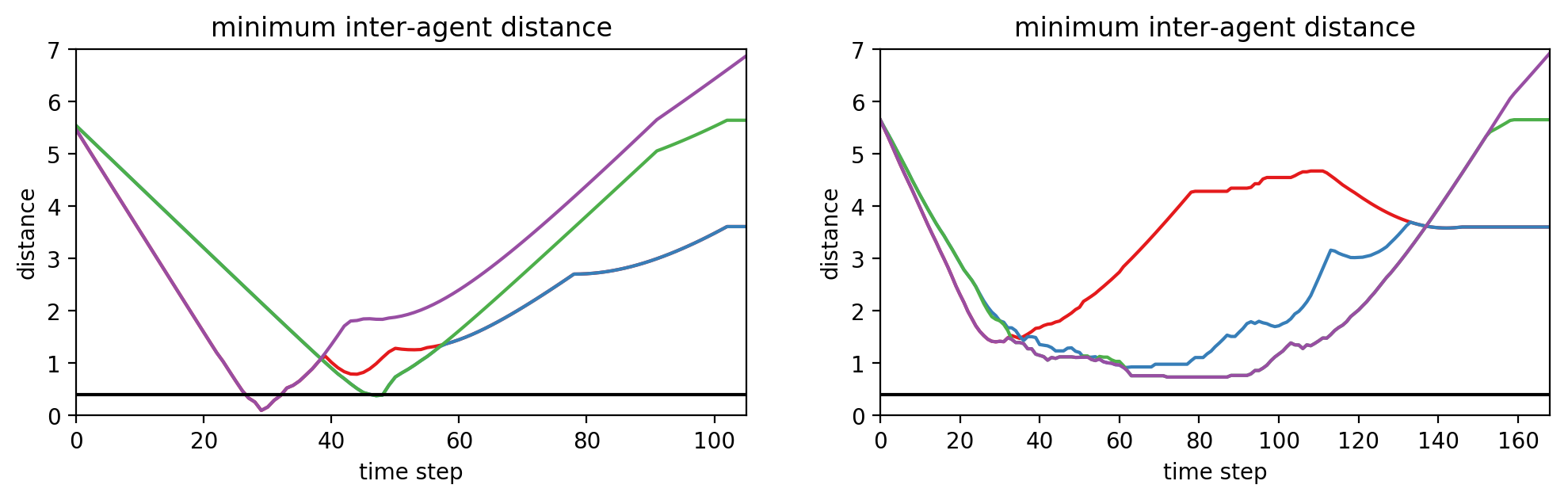
Figure 4: Inter-agent distances RVO (left) and our method (right). The RVO simulation results in inter-agent distances below the collision threshold (black line).

Figure 5 shows six instances of a 3D simulation with 10 agents. The agents start at the sides of a $10$\mathrm{m}$\times 10$\mathrm{m}$\times 10$\mathrm{m}$$ cube and are constrained to a maximum speed of $6$\mathrm{m}\mathrm{/}\mathrm{s}$$ and a maximum measurement error set to $1.0$\mathrm{m}$$. The algorithm was run at $60$\mathrm{Hz}$$. The agents, displayed as quadrotors, each have a bounding box of $0.45$\mathrm{m}$\times 0.45$\mathrm{m}$\times 0.2$\mathrm{m}$$ and an additional ellipsoidal margin with axis lengths of $.3$\mathrm{m}$$ in the $x$ and $y$ dimensions, and $1.2$\mathrm{m}$$ in the $z$ dimension. This margin effectively gives a buffer of $0.75$\mathrm{m}$$ in the $xy$ plane and a large buffer of $1.3$\mathrm{m}$$ in $z$. We assume non-spherical margins in this simulation since, in the case of quadrotor flight, large margins in the $z$ direction can prevent unwanted effects due to downwash [PHAS17]. The minimum inter-agent distance during the simulation, as measured from the centers of the agents, was $1.6$\mathrm{m}$$.

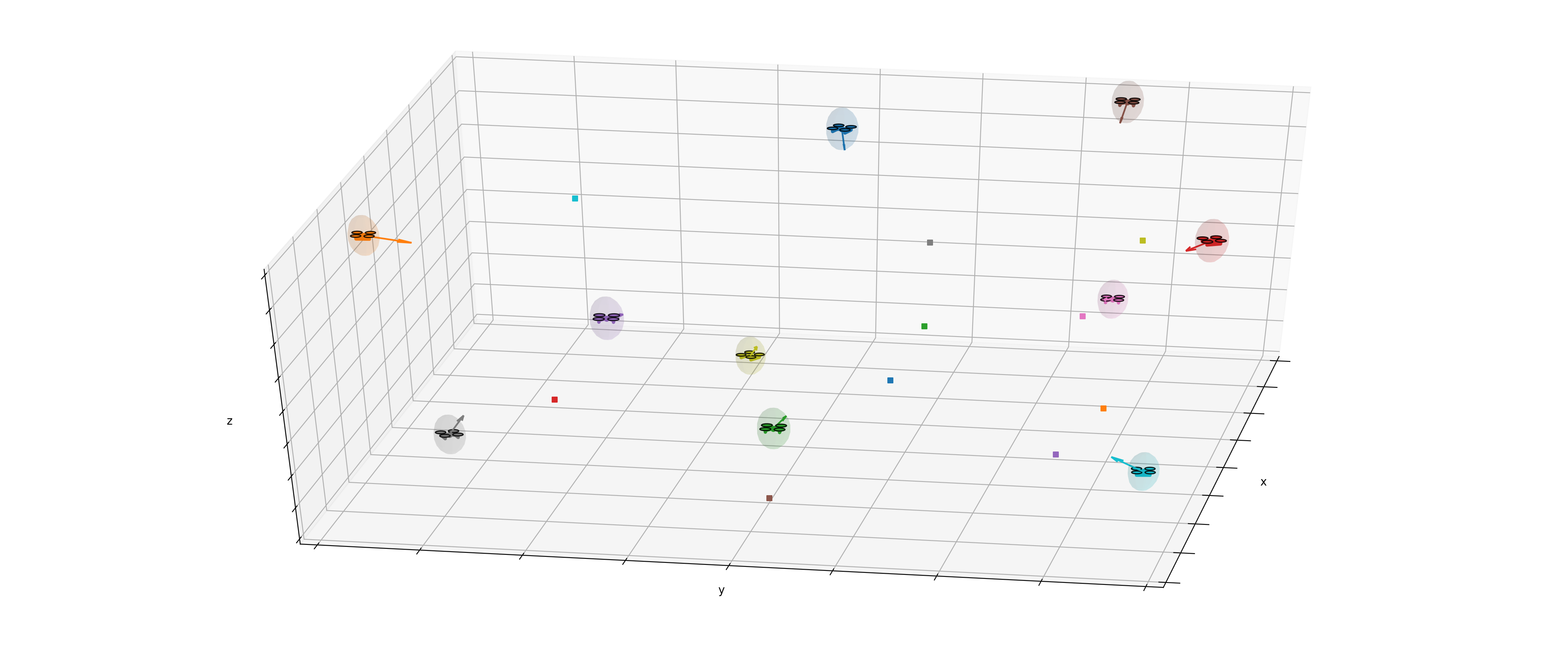
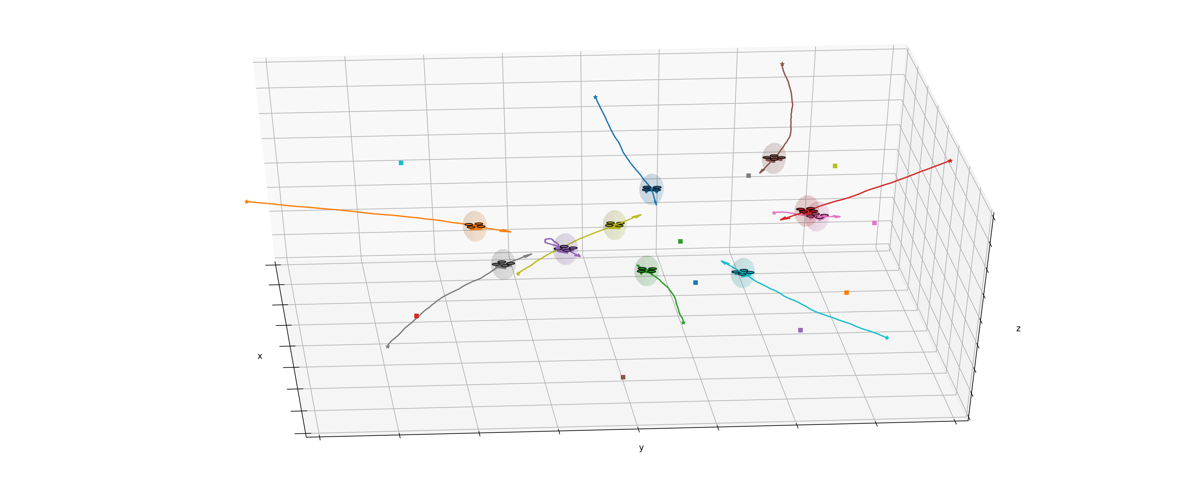
$t=0\hskip 144.54ptt=60$
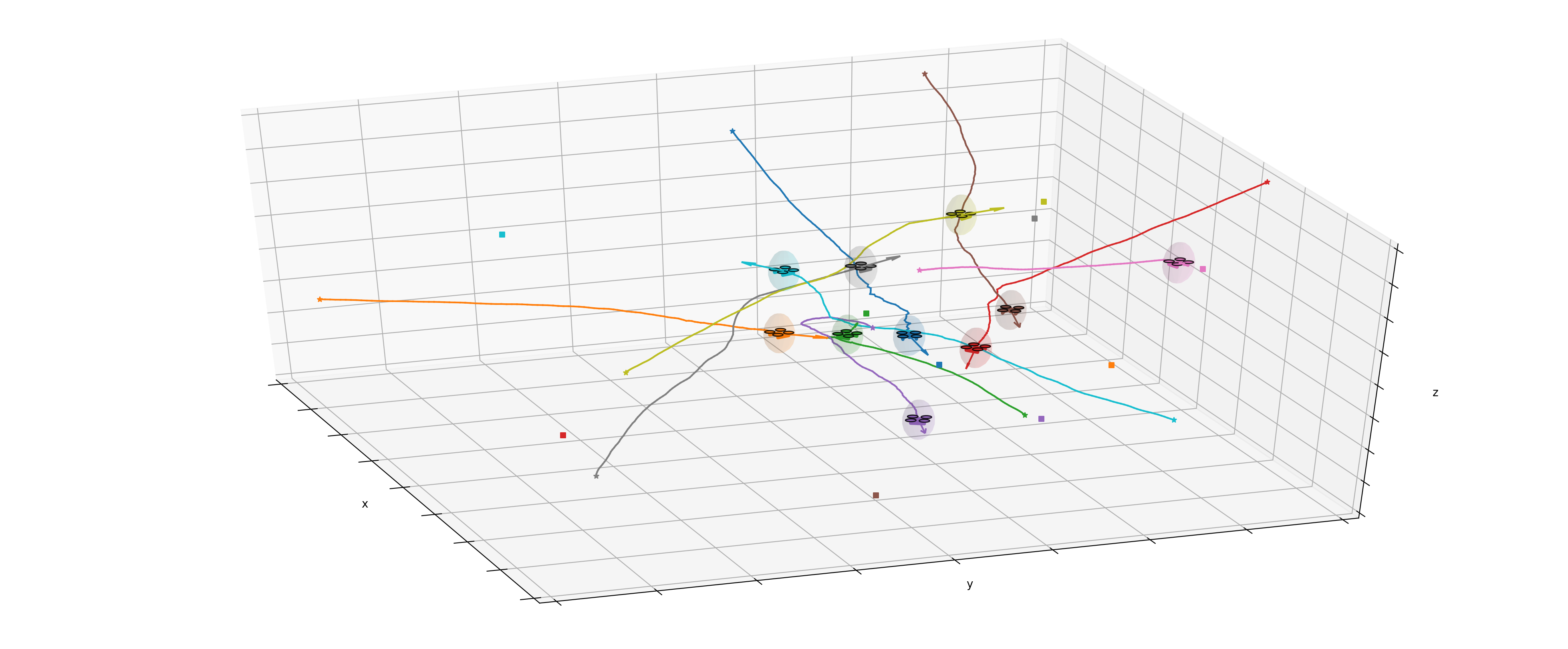
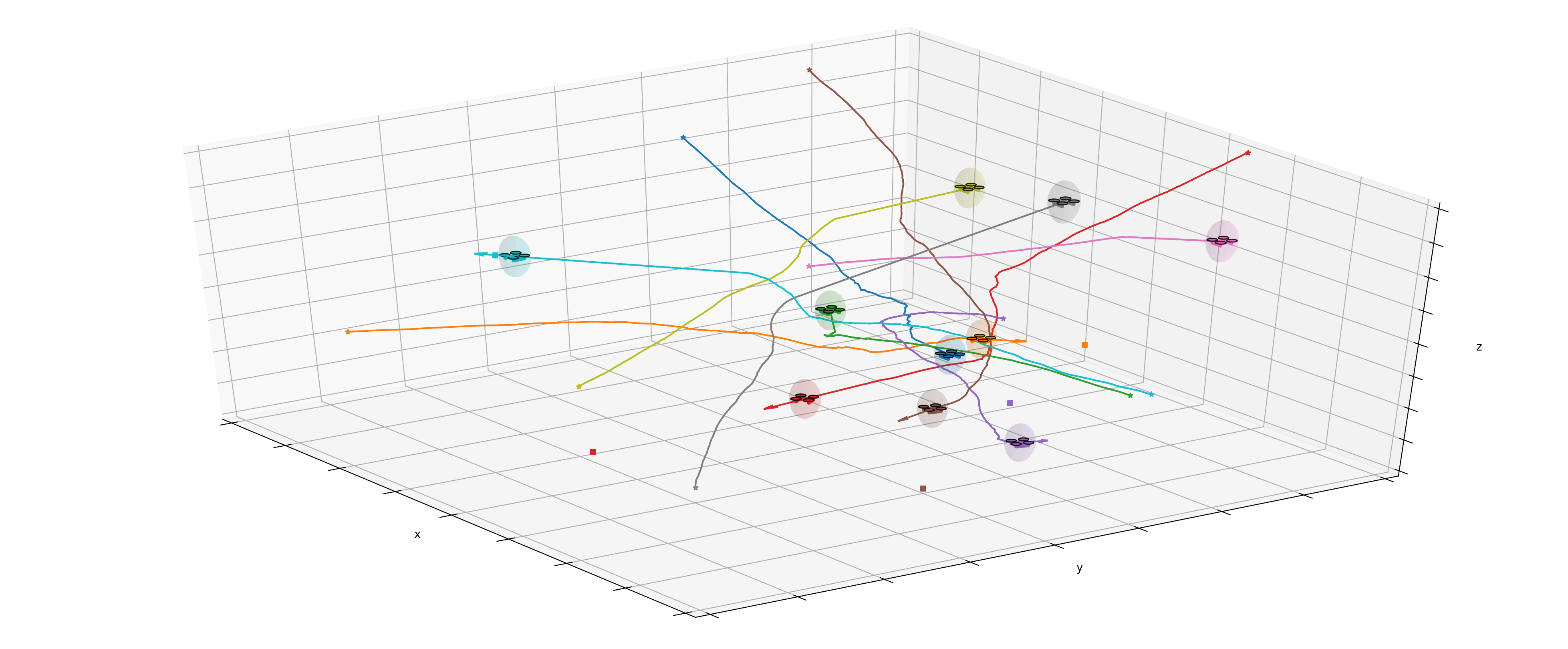
$t=120\hskip 144.54ptt=180$
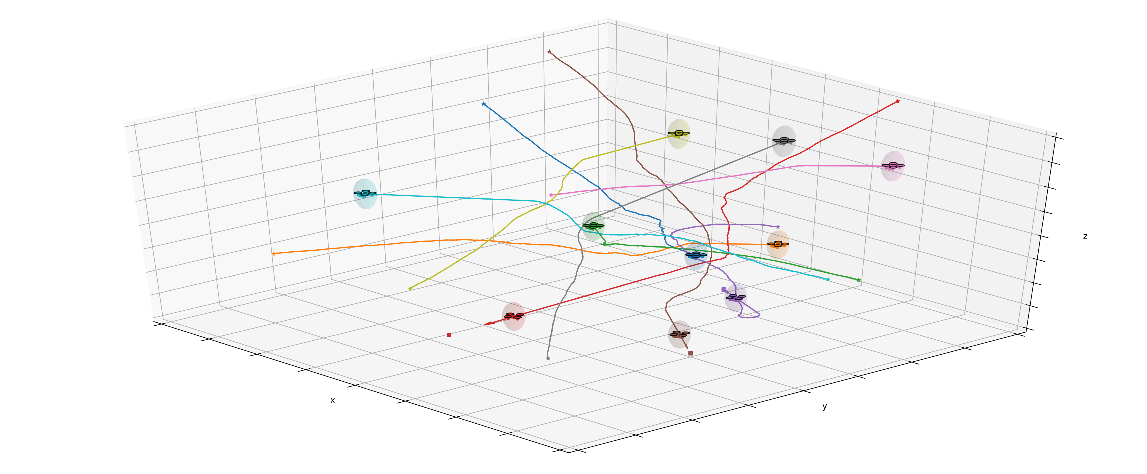
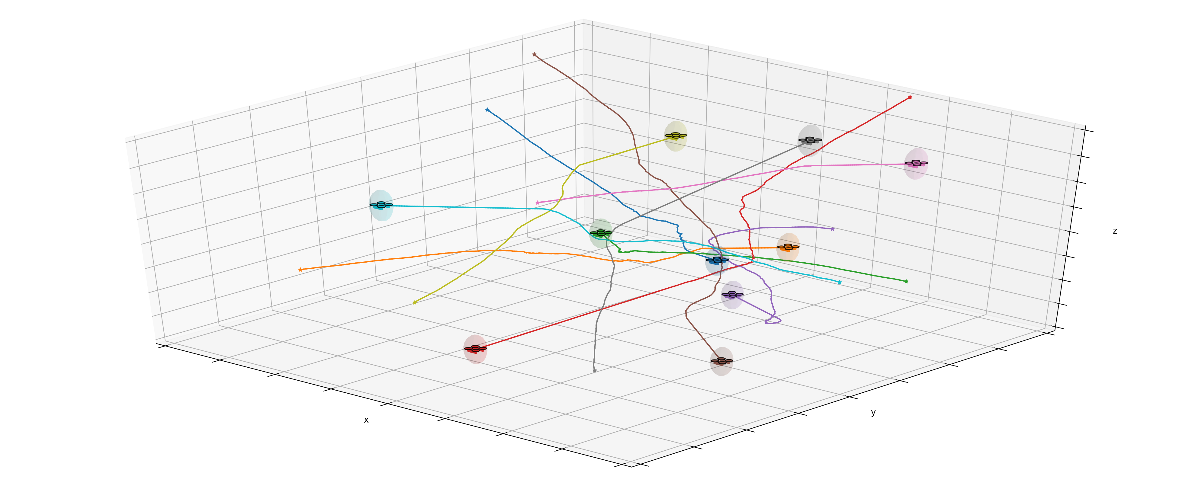
$t=210\hskip 144.54ptt=232$

Figure 5: Six time instances of a 3D simulation of 10 agents. Each agent adds an ellipsoidal margin (shown) elongated in the z-axis to account for downwash affects.

6 Closing Remarks

While cloud and edge computing has relieved many of the burdens distributed robotic systems encounter, network delays, disconnects, and other failures are still commonplace at scale. Dependable and fast algorithms that can run onboard are, therefore, critical for any certifiable system. In this work, we presented a scalable system that can work with simple or complex, distributed or centralized high level planers to provide safe trajectories for a group of agents. Under the assumptions stated, we showed that collision avoidance is guaranteed, provided each agent follows this method. However, we observe practical collision avoidance behavior even if only the ego agent follows this method. Computational performance results and simulations provide evidence that this algorithm can potentially be used in safety-critical applications for mobile robots with simple dynamics.

Future work will focus on creating a fast, easily extendable library for automatically generating programs of the form of problem (12), by making use of the composition rules presented in the appendix. We suspect that future support for warm starts and the ability to change parameters without reconstructing the complete problem from scratch (as compared to §5.1) would yield a substantial speed up in solution time. Additionally, we note that while immediately attempting to use problem (12) in a Model Predictive Control (MPC) formalism yields a nonconvex problem, we believe that there may be a approach to approximate solution while retaining the feasibility properties assumed in (5). We also plan on incorporating a global planner, which can handle static obstacles less conservatively than our algorithm, into our trajectory planning pipeline.

7 Appendix

7.1 Dual functions

In this subsection, we derive the Lagrange dual function for the Voronoi cell generated by polyhedra.

Polyhedra.

In the case where our set $\mathcal{E}$ is specified by an affine constraint (i.e., $\mathcal{E}$ is a polyhedron),

$$\mathcal{E}=\{y~{}|~{}Ay\leq b\},$$

with $A\in{\mbox{\bf R}}^{m\times n}$ and $b\in{\mbox{\bf R}}^{m}$, then the dual function can be easily computed.

First, note that the minimizer of $\left\|{y}\right\|_{2}^{2}-2c^{T}y$ can be found by setting the gradient to zero (this is necessary and sufficient by convexity and differentiability), which yields that the optimal point is $y^{*}=c$, with optimal value

$$\inf_{y}\left(\left\|{y}\right\|_{2}^{2}+2c^{T}y\right)=-\left\|{c}\right\|_{2}^{2}.$$

Applying this result yields

$$g(x,\lambda)=\inf_{y}\left(\left\|{y}\right\|_{2}^{2}-2x^{T}y+\lambda^{T}(Ay-b)\right)=-\left\|{x-A^{T}\lambda/2}\right\|_{2}^{2}-b^{T}\lambda,$$

with $\lambda\geq 0$.

7.2 Extensions

There are several natural extensions to problem (8). These extensions can be combined, as needed.

Union of convex sets.

We can extend the formalism of (8) to include the Voronoi region generated by a finite union of convex sets. That is, if $S$ can be written in the form

$$S=\bigcup_{i=1}^{\ell}~{}\{y~{}|~{}f_{i}(y)\leq 0\},$$

for convex functions $f_{i}:{\mbox{\bf R}}^{n}\to{\mbox{\bf R}}^{m_{i}}$. Note that, in general, $S$ will not be convex, while the resulting Voronoi region always is, since the region is the intersection of a family of hyperplanes. Additionally, we will require that there exist $y_{i}^{0}\in{\mbox{\bf R}}^{n}$ with $f_{i}(y_{i}^{0})<0$ for $i=1,\dots,\ell$ if $f_{i}$ is not affine. The corresponding problem is given by

$$\begin{array}[]{ll}\mbox{minimize}&\left\|{x-x^{\mathrm{g}}}\right\|_{2}^{2}\\ \mbox{subject to}&\left\|{x^{\mathrm{c}}}\right\|_{2}^{2}-2x^{T}x^{\mathrm{c}}\leq\inf_{f_{i}(y)\leq 0}\left(\left\|{y}\right\|_{2}^{2}-2y^{T}x\right),~{}~{}i=1,\dots,\ell.\end{array}$$

In this case, we simply derive a dual function for each constraint with $i=1,\dots,\ell$, writing each as a constraint as in (10), each of which is convex.

Intersection of a convex set with the Voronoi cell.

Given a convex set $C$ specified by

$$C=\{x~{}|~{}h(x)\leq 0\},$$

where $h:{\mbox{\bf R}}^{n}\to{\mbox{\bf R}}^{r}$ is a convex function, then the problem

$$\begin{array}[]{ll}\mbox{minimize}&\left\|{x-x^{\mathrm{g}}}\right\|_{2}^{2}\\ \mbox{subject to}&\left\|{x^{\mathrm{c}}}\right\|_{2}^{2}-2x^{T}x^{\mathrm{c}}\leq\inf_{f(y)\leq 0}\left(\left\|{y}\right\|_{2}^{2}-2y^{T}x\right)\\ &h(x)\leq 0,\end{array}$$

is the intersection of the Voronoi cell in question and the set $C$, which is also easily solvable assuming $h$ can be easily evaluated at any point in its domain.

References

- [ASD12] F. Augugliaro, A. P. Schoellig, and R. D’Andrea. Generation of collision-free trajectories for a quadrocopter fleet: A sequential convex programming approach. In 2012 IEEE/RSJ International Conference on Intelligent Robots and Systems, pages 1917–1922, Oct 2012.
- [AVDB18] Akshay Agrawal, Robin Verschueren, Steven Diamond, and Stephen Boyd. A rewriting system for convex optimization problems. Journal of Control and Decision, 5(1):42–60, 2018.
- [BCH14] S. Bandyopadhyay, S. Chung, and F. Y. Hadaegh. Probabilistic swarm guidance using optimal transport. In 2014 IEEE Conference on Control Applications (CCA), pages 498–505, Oct 2014.
- [BEKS17] Jeff Bezanson, Alan Edelman, Stefan Karpinski, and Viral B. Shah. Julia: A fresh approach to numerical computing. SIAM review, 59(1):65–98, 2017.
- [BR71] D. Bertsekas and I. Rhodes. Recursive state estimation for a set-membership description of uncertainty. IEEE Transactions on Automatic Control, 16(2):117–128, Apr 1971.
- [BV04] Stephen Boyd and Lieven Vandenberghe. Convex optimization. Cambridge university press, 2004.
- [CCH15] Yufan Chen, Mark Cutler, and Jonathan P How. Decoupled multiagent path planning via incremental sequential convex programming. In 2015 IEEE International Conference on Robotics and Automation (ICRA), pages 5954–5961. IEEE, 2015.
- [CHTM12] D. Claes, D. Hennes, K. Tuyls, and W. Meeussen. Collision avoidance under bounded localization uncertainty. In 2012 IEEE/RSJ International Conference on Intelligent Robots and Systems, pages 1192–1198, Oct 2012.
- [CR16] Jiahao Chen and Jarrett Revels. Robust benchmarking in noisy environments. arXiv preprint arXiv:1608.04295, 2016.
- [DCB13] Alexander Domahidi, Eric Chu, and Stephen Boyd. Ecos: An socp solver for embedded systems. In 2013 European Control Conference (ECC), pages 3071–3076. IEEE, 2013.
- [DHL17] Iain Dunning, Joey Huchette, and Miles Lubin. JuMP: A modeling language for mathematical optimization. SIAM Review, 59(2):295–320, 2017.
- [GSK+17] B. Gopalakrishnan, A. K. Singh, M. Kaushik, K. M. Krishna, and D. Manocha. Prvo: Probabilistic reciprocal velocity obstacle for multi robot navigation under uncertainty. In 2017 IEEE/RSJ International Conference on Intelligent Robots and Systems (IROS), pages 1089–1096, Sep. 2017.
- [HZZ+12] Haomiao Huang, Zhengyuan Zhou, Wei Zhang, Jerry Ding, Dušan M Stipanovic, and Claire J Tomlin. Safe-reachable area cooperative pursuit. IEEE Transactions on Robotics, 2012.
- [JSCP15] Lucas Janson, Edward Schmerling, Ashley Clark, and Marco Pavone. Fast marching tree: A fast marching sampling-based method for optimal motion planning in many dimensions. The International Journal of Robotics Research, 34(7):883–921, 2015.
- [LVBL98] Miguel S. Lobo, Lieven Vandenberghe, Stephen Boyd, and Hervé Lebret. Applications of second-order cone programming. Linear algebra and its applications, 284(1-3):193–228, 1998.
- [LZW16] Yushuang Liu, Yan Zhao, and Falin Wu. Ellipsoidal state-bounding-based set-membership estimation for linear system with unknown-but-bounded disturbances. IET Control Theory & Applications, 10(4):431–442, feb 2016.
- [MCH14] Daniel Morgan, Soon-Jo Chung, and Fred Y Hadaegh. Model predictive control of swarms of spacecraft using sequential convex programming. Journal of Guidance, Control, and Dynamics, 37(6):1725–1740, 2014.
- [MJWP16] X. Ma, Z. Jiao, Z. Wang, and D. Panagou. Decentralized prioritized motion planning for multiple autonomous uavs in 3d polygonal obstacle environments. In 2016 International Conference on Unmanned Aircraft Systems (ICUAS), pages 292–300, June 2016.
- [PHAS17] J. A. Preiss, W. Hönig, N. Ayanian, and G. S. Sukhatme. Downwash-aware trajectory planning for large quadrotor teams. In 2017 IEEE/RSJ International Conference on Intelligent Robots and Systems (IROS), pages 250–257, Sep. 2017.
- [ŞHA19] Baskın Şenbaşlar, Wolfgang Hönig, and Nora Ayanian. Robust trajectory execution for multi-robot teams using distributed real-time replanning. In Distributed Autonomous Robotic Systems, pages 167–181. Springer, 2019.
- [SHL+13] John Schulman, Jonathan Ho, Alex X Lee, Ibrahim Awwal, Henry Bradlow, and Pieter Abbeel. Finding locally optimal, collision-free trajectories with sequential convex optimization. In Robotics: science and systems, volume 9, pages 1–10. Citeseer, 2013.
- [SS19] Kunal Shah and Mac Schwager. Multi-agent cooperative pursuit-evasion strategies under uncertainty. In Distributed Autonomous Robotic Systems, pages 451–468. Springer, 2019.
- [UG18] Alexei Yu Uteshev and Marina V Goncharova. Point-to-ellipse and point-to-ellipsoid distance equation analysis. Journal of Computational and Applied Mathematics, 328:232–251, 2018.
- [VdBGLM11] Jur Van den Berg, Stephen Guy, Ming Lin, and Dinesh Manocha. Reciprocal n-Body Collision Avoidance, volume 70, pages 3–19. 04 2011.
- [VdBGS+16] Jur Van den Berg, Stephen Guy, Jamie Snape, Ming Lin, and Manocha. Rvo2 library: Reciprocal collision avoidance for real-time multi-agent simulation, 2016.
- [VdBLM08] Jur Van den Berg, Ming Lin, and Dinesh Manocha. Reciprocal velocity obstacles for real-time multi-agent navigation. In 2008 IEEE International Conference on Robotics and Automation, pages 1928–1935. IEEE, 2008.
- [Wat81] David F Watson. Computing the n-dimensional delaunay tessellation with application to voronoi polytopes. The computer journal, 24(2):167–172, 1981.
- [WC11] G. Wagner and H. Choset. M*: A complete multirobot path planning algorithm with performance bounds. In 2011 IEEE/RSJ International Conference on Intelligent Robots and Systems, pages 3260–3267, Sep. 2011.
- [ZA19] H. Zhu and J. Alonso-Mora. Chance-constrained collision avoidance for mavs in dynamic environments. IEEE Robotics and Automation Letters, 4(2):776–783, 2019.
- [ZWBS17] Dingjiang Zhou, Zijian Wang, Saptarshi Bandyopadhyay, and Mac Schwager. Fast, on-line collision avoidance for dynamic vehicles using buffered voronoi cells. IEEE Robotics and Automation Letters, 2(2):1047–1054, 2017.