Ab initio theory of the spin-dependent conductivity tensor and the spin Hall effect in random alloys

Abstract

We present an extension of the relativistic electron transport theory for the standard (charge) conductivity tensor of random alloys within the tight-binding linear muffin-tin orbital method to the so-called spin-dependent conductivity tensor, which describes the Kubo linear response of spin currents to external electric fields. The approach is based on effective charge- and spin-current operators, that correspond to intersite electron transport and that are nonrandom, which simplifies the configuration averaging by means of the coherent potential approximation. Special attention is paid to the Fermi sea term of the spin-dependent conductivity tensor, which contains a nonzero incoherent part, in contrast to the standard conductivity tensor. The developed formalism is applied to the spin Hall effect in binary random nonmagnetic alloys, both on a model level and for Pt-based alloys with an fcc structure. We show that the spin Hall conductivity consists of three contributions (one intrinsic and two extrinsic) which exhibit different concentration dependences in the dilute limit of an alloy. Results for selected Pt alloys (Pt-Re, Pt-Ta) lead to the spin Hall angles around 0.2; these sizable values are obtained for compositions that belong to thermodynamically equilibrium phases. These alloys can thus be considered as an alternative to other systems for efficient charge to spin conversion, which are often metastable crystalline or amorphous alloys.

I Introduction

Efficient generation and reliable detection of spin currents in magnetoelectronic devices belong to the central topics of the whole area of spintronics Maekawa et al. (2012); Tsymbal and Žutić (2012). In systems without local magnetic moments and in the absence of external magnetic fields, the most important phenomenon in this context is undoubtedly the spin Hall effect (SHE) Sinova et al. (2015). This transport phenomenon was predicted as a consequence of spin-orbit interaction Hirsch (1999); subsequent systematic theoretical and experimental investigation resulted in detailed understanding of its basic aspects.

In pure metals and ordered crystals, the SHE arises solely due to the band structure of the system, i.e., due to the dependence of energy eigenvalues and eigenvectors on the reciprocal-space vector $\mathbf{k}$, without the need of any explicit mechanism of electron scattering. The central quantity, namely the intrinsic spin Hall conductivity (SHC), can be expressed in terms of the Berry curvature of the occupied electron states Guo et al. (2008); Freimuth et al. (2010). In diluted metallic alloys, the impurity scattering leads to an extrinsic contribution to the SHC that can be treated on different levels of sophistication of electron transport theory. The extrinsic SHC is due to the skew-scattering and side-jump mechanisms whereby the former one dominates in the dilute limit. Evaluation of the extrinsic contribution within the linearized Boltzmann equation rests on the scattering-in terms Gradhand et al. (2010) while the Kubo linear response theory with the coherent potential approximation (CPA) requires inclusion of the so-called vertex corrections Lowitzer et al. (2011).

The intrinsic and extrinsic contributions to the SHC have its counterparts in a description of the anomalous Hall effect in ferromagnetic systems Nagaosa et al. (2010); Zimmermann et al. (2014), so that similar concepts appear in studies of both transverse transport phenomena. In the SHE, the relative magnitude of the SHC is expressed by the so-called spin Hall angle (SHA), defined as a ratio of the SHC to the standard (charge) longitudinal conductivity. The SHA represents a dimensionless measure of efficiency of the charge to spin conversion. For this reason, both experimental and theoretical effort has recently been devoted to find systems with large SHA, see, e.g., Refs. Chadova et al., 2015a; Obstbaum et al., 2016 and references therein. Besides the usual bulk metals and diluted and concentrated alloys containing heavy elements, large spin Hall currents can be induced by Rashba interface effects Wang et al. (2016); Borge and Tokatly (2017); Amin et al. (2018); Li et al. (2019); Wesselink et al. (2019). Further manifestation of spin-orbit effects in nonmagnetic solids is a possible spin polarization of longitudinal currents due to a special point group symmetry of the crystal structure Wimmer et al. (2015).

Spin currents in systems with spontaneous magnetic moments represent another wide area of the present intense research. This field includes spin-transfer torques in layered systems Ralph and Stiles (2008), spin polarization of longitudinal Lowitzer et al. (2010) and transversal Zimmermann et al. (2014) conductivities in bulk ferromagnetic alloys, as well as the SHE in collinear Freimuth et al. (2010) and noncollinear Zhang et al. (2017) antiferromagnets. The latter systems have attracted special interest since their noncollinear spin structures can induce a sizable SHE even without spin-orbit interaction Zhang et al. (2018).

Reliable quantum-mechanical description of phenomena related to the spin currents faces a basic problem due to the fact that the electron spin in systems with spin-orbit interaction is not a conserving quantity. This hinders an exact definition of the spin-current operator; fundamental approaches to this problem Wang et al. (2006); Shi et al. (2006) lead to expressions that cannot be employed directly in current ab initio techniques of electron theory of solids. In this situation, existing practical solutions thus express the spin-current operator typically as a symmetrized product of the spin operator and the operator of charge current Guo et al. (2008); Lowitzer et al. (2010); Wang et al. (2016). It should be noted that the latter approaches are suitable even for studies of disordered systems, in which the necessary configuration averaging is performed either by a real-space supercell technique Wang et al. (2016) or by using the CPA Lowitzer et al. (2011, 2010).

The main aim of this work is a formulation of an alternative first-principles approach to the spin currents in random alloys which employs the idea of an intersite electron transport Turek et al. (2002). In this scheme, the intraatomic electron motion is systematically neglected which leads to effective operators of charge current that are spin-independent and nonrandom (independent of a particular random configuration of the alloy). The corresponding effective spin-current operators are nonrandom as well, which allows us to define easily the spin-dependent conductivity tensor and to perform its configuration averaging within the single-site CPA Soven (1967); Velický (1969) in analogy with the technique developed recently for the standard (charge) conductivity tensor in relativistic theory Turek et al. (2012, 2014).

The paper is organized as follows. The theoretical formalism is presented in Section II, including the definition of the spin-dependent conductivity tensor (Section II.1), the CPA averaging of its Fermi sea term (Section II.2), a summary of the formal properties of the derived theory (Section II.3), and details of numerical implementation (Section II.4). Technical theoretical details are presented in the Appendix A. The obtained results and their discussion, focused on the SHE in nonmagnetic random alloys, are collected in Section III. First, a simple tight-binding model of a random binary alloy is analyzed in the dilute limit in Section III.1. Second, transport properties of selected Pt-based disordered fcc alloys (Pt-Au, Pt-Re, Pt-Ta) are addressed in Section III.2. Conclusions of the work are summarized in Section IV.

II Method

II.1 Spin-dependent conductivity tensor from the Bastin formula

The starting point of our formalism is the Kubo linear response theory Kubo (1957) and the formula of Bastin et al. Bastin et al. (1971) for the full charge conductivity tensor $\sigma_{\mu\nu}$ adapted in the relativistic tight-binding linear muffin-tin orbital (TB-LMTO) method Turek et al. (2014)

$$\sigma_{\mu\nu} = -2\sigma_{0}\int\mathrm{d}Ef(E)\mathrm{Tr}\left\langle v_{\mu}g^{\prime}_{+}(E)v_{\nu}[g_{+}(E)-g_{-}(E)]\right.$$ (1)

$$\left.\qquad\qquad\qquad\quad\ {}-v_{\mu}[g_{+}(E)-g_{-}(E)]v_{\nu}g^{\prime}_{-}(E)\right\rangle.$$

In this relation, the quantity $\sigma_{0}=e^{2}\hbar/(4\pi\Omega)$, where $\Omega$ is the volume of a big finite crystal with periodic boundary conditions, $E$ is a real energy variable, $f(E)$ denotes the Fermi-Dirac function, $g_{\pm}(E)=g(E\pm i0)$ denote side limits of the auxiliary Green’s function $g(z)$ defined for complex energies $z$, the prime at $g_{\pm}(E)$ denotes energy derivative, the quantities $v_{\mu}$ ($\mu=x,y,z$) are the effective velocity (current) operators, and the brackets $\langle\dots\rangle$ refer to the configuration averaging for random alloys. The auxiliary Green’s function is given as $g(z)=[P(z)-S]^{-1}$, where $P(z)$ represents a site-diagonal matrix of the potential functions and $S$ denotes the structure constant matrix.

The expression (1) reflects the intersite electron transport which takes place inside the interstitial region among the individual Wigner-Seitz cells (replaced by space-filling spheres in the atomic-sphere approximation). The operators $v_{\mu}$ and $g_{\pm}(E)$ are represented by matrices in the composed index $\mathbf{R}L$, where $\mathbf{R}$ labels the lattice sites and $L$ denotes the orbital index $L=(\ell ms)$ containing the orbital ($\ell$), magnetic ($m$), and spin ($s$) quantum numbers ($s=\,\uparrow,\downarrow$). The trace ($\mathrm{Tr}$) in Eq. (1) refers to all $\mathbf{R}L$-orbitals of the system. Note that the orbital index $L$ corresponds to a nonrelativistic theory despite that the fully relativistic solutions (including possible spin polarization) of the single-site problem are used inside the Wigner-Seitz cells (atomic spheres); this fact is due to the nonrelativistic form of the LMTO orbitals in the interstitial region (which reduce to spherical waves in a constant potential with zero kinetic energy Andersen (1975); Andersen and Jepsen (1984)). The effective current operators $v_{\mu}$ are spin-independent and nonrandom which follows from their definition Turek et al. (2002, 2014) and from properties of the structure constant matrix $S$.

The nonrelativistic character of the intersite electron transport and the above properties of the effective current operators $v_{\mu}$ allow one to introduce naturally the effective spin-current operators as $\sigma^{\lambda}v_{\mu}$, where the quantities $\sigma^{\lambda}$ ($\lambda=x,y,z$) equal the Pauli spin matrices extended trivially to matrices in the composed $\mathbf{R}L$ index, $(\sigma^{\lambda})^{L^{\prime}L}_{\mathbf{R}^{\prime}\mathbf{R}}=\delta_{\mathbf{R}^{\prime}\mathbf{R}}\delta_{\ell^{\prime}\ell}\delta_{m^{\prime}m}\sigma^{\lambda}_{s^{\prime}s}$ where $L^{\prime}=(\ell^{\prime}m^{\prime}s^{\prime})$. This definition represents an analogy of spin-current operators employed in other studies Guo et al. (2008); Lowitzer et al. (2010); Wang et al. (2016). The spin-dependent conductivity tensor $\sigma^{\lambda}_{\mu\nu}$ corresponding to the original charge conductivity tensor (1) is then defined by

$$\sigma^{\lambda}_{\mu\nu} = -2\sigma_{0}\int\mathrm{d}Ef(E)\mathrm{Tr}\left\langle(\sigma^{\lambda}v_{\mu})g^{\prime}_{+}(E)v_{\nu}[g_{+}(E)-g_{-}(E)]\right.$$ (2)

$$\left.\qquad\qquad\qquad\quad\ {}-(\sigma^{\lambda}v_{\mu})[g_{+}(E)-g_{-}(E)]v_{\nu}g^{\prime}_{-}(E)\right\rangle,$$

which describes the linear response of the spin current $\sigma^{\lambda}v_{\mu}$ to a spin-independent electrical field in the direction of the $\nu$ axis. Alternatively, one can consider the response coefficient

$$\tilde{\sigma}_{\mu\nu} = -2\sigma_{0}\int\mathrm{d}Ef(E)\mathrm{Tr}\left\langle\tilde{v}_{\mu}g^{\prime}_{+}(E)v_{\nu}[g_{+}(E)-g_{-}(E)]\right.$$ (3)

$$\left.\qquad\qquad\qquad\quad\ {}-\tilde{v}_{\mu}[g_{+}(E)-g_{-}(E)]v_{\nu}g^{\prime}_{-}(E)\right\rangle,$$

where $\tilde{v}_{\mu}=({\bf n}\cdot\bm{\sigma})v_{\mu}$ denotes the spin-polarized effective velocity (current) with the spin-polarization axis along a global nonrandom unit vector ${\bf n}$. Note that the spin-polarized velocities $\tilde{v}_{\mu}$ are nonrandom operators, which simplifies the configuration averaging in Eq. (3).

In full analogy to $\sigma_{\mu\nu}$, the spin-dependent conductivity tensor $\tilde{\sigma}_{\mu\nu}$ can be decomposed into a Fermi surface term and a Fermi sea term as Turek et al. (2014); Crépieux and Bruno (2001)

$$\tilde{\sigma}_{\mu\nu}=\tilde{\sigma}^{(1)}_{\mu\nu}+\tilde{\sigma}^{(2)}_{\mu\nu}.$$ (4)

For systems at zero temperature, the Fermi surface term $\tilde{\sigma}^{(1)}_{\mu\nu}$ can be written as

$$\tilde{\sigma}^{(1)}_{\mu\nu} = \sigma_{0}\mathrm{Tr}\left\langle\tilde{v}_{\mu}[g_{+}(E_{\mathrm{F}})-g_{-}(E_{\mathrm{F}})]v_{\nu}g_{-}(E_{\mathrm{F}})\right.$$ (5)

$$\left.\quad\ {}-\tilde{v}_{\mu}g_{+}(E_{\mathrm{F}})v_{\nu}[g_{+}(E_{\mathrm{F}})-g_{-}(E_{\mathrm{F}})]\right\rangle,$$

where $E_{\mathrm{F}}$ denotes the Fermi energy. The Fermi sea term $\tilde{\sigma}^{(2)}_{\mu\nu}$ can be reformulated as a complex contour integral

$$\tilde{\sigma}^{(2)}_{\mu\nu}=\sigma_{0}\int_{C}\mathrm{d}z\mathrm{Tr}\langle\tilde{v}_{\mu}g^{\prime}(z)v_{\nu}g(z)-\tilde{v}_{\mu}g(z)v_{\nu}g^{\prime}(z)\rangle,$$ (6)

where the integration path $C$ starts and ends at $E_{\mathrm{F}}$, it is oriented counterclockwise and it encompasses the whole occupied part of the alloy valence spectrum.

The configuration average in the CPA of the Fermi surface term yields its coherent part (coh) and the incoherent part (vertex corrections – VC), $\tilde{\sigma}^{(1)}_{\mu\nu}=\tilde{\sigma}^{(1)}_{\mu\nu,\mathrm{coh}}+\tilde{\sigma}^{(1)}_{\mu\nu,\mathrm{VC}}$, where

$$\tilde{\sigma}^{(1)}_{\mu\nu,\mathrm{coh}} = \sigma_{0}\mathrm{Tr}\left\{\tilde{v}_{\mu}[\bar{g}_{+}(E_{\mathrm{F}})-\bar{g}_{-}(E_{\mathrm{F}})]v_{\nu}\bar{g}_{-}(E_{\mathrm{F}})\right.$$ (7)

$$\left.\quad\ {}-\tilde{v}_{\mu}\bar{g}_{+}(E_{\mathrm{F}})v_{\nu}[\bar{g}_{+}(E_{\mathrm{F}})-\bar{g}_{-}(E_{\mathrm{F}})]\right\},$$

while the vertex corrections $\tilde{\sigma}^{(1)}_{\mu\nu,\mathrm{VC}}$ are evaluated according to the original CPA theory Velický (1969) adapted to the TB-LMTO formalism Carva et al. (2006). The symbols $\bar{g}_{\pm}(E)$ in Eq. (7) and $\bar{g}(z)$ in the following text denote the configuration averages of $g_{\pm}(E)$ and $g(z)$, respectively. These quantities are given by $\bar{g}(z)=[\mathcal{P}(z)-S]^{-1}$, where $\mathcal{P}(z)$ is a site-diagonal matrix of the coherent potential functions. The treatment of the Fermi sea term (6) is done similarly to the case of the charge conductivity tensor Turek et al. (2014); the details are given in Section II.2.

II.2 Configuration averaging of the Fermi sea term

In analogy with our recent study Turek et al. (2014), we find that the CPA average of the Fermi sea term (6) can be simplified owing to the exact vanishing of the on-site blocks of the matrix product $\bar{g}(z)v_{\nu}\bar{g}(z)$:

$$[\bar{g}(z)v_{\nu}\bar{g}(z)]^{LL^{\prime}}_{\mathbf{R}\mathbf{R}}=0,$$ (8)

which is valid for the same energy arguments of both Green’s functions. This rule is a consequence of a simple form of the underlying coordinate operators and of the single-site nature of the coherent potential functions $\mathcal{P}(z)$, see Ref. Turek et al., 2014 for details. Following the procedure outlined previously Turek et al. (2014), one can derive the resulting averages in Eq. (6) as

$$\mathrm{Tr}\langle\tilde{v}_{\mu}g^{\prime}v_{\nu}g\rangle=\mathrm{Tr}\{\tilde{v}_{\mu}\bar{g}^{\prime}v_{\nu}\bar{g}\}+\sum_{\mathbf{R}_{1}\Lambda_{1}}\sum_{\mathbf{R}_{2}\Lambda_{2}}\left[\bar{g}\tilde{v}_{\mu}\bar{g}\right]^{L^{\prime}_{1}L_{1}}_{\mathbf{R}_{1}\mathbf{R}_{1}}\left[\Delta^{-1}\right]^{\Lambda_{1}\Lambda_{2}}_{\mathbf{R}_{1}\mathbf{R}_{2}}\left[\bar{g}^{\prime}v_{\nu}\bar{g}\right]^{L_{2}L^{\prime}_{2}}_{\mathbf{R}_{2}\mathbf{R}_{2}}$$ (9)

and

$$\mathrm{Tr}\langle\tilde{v}_{\mu}gv_{\nu}g^{\prime}\rangle=\mathrm{Tr}\{\tilde{v}_{\mu}\bar{g}v_{\nu}\bar{g}^{\prime}\}+\sum_{\mathbf{R}_{1}\Lambda_{1}}\sum_{\mathbf{R}_{2}\Lambda_{2}}\left[\bar{g}\tilde{v}_{\mu}\bar{g}\right]^{L^{\prime}_{1}L_{1}}_{\mathbf{R}_{1}\mathbf{R}_{1}}\left[\Delta^{-1}\right]^{\Lambda_{1}\Lambda_{2}}_{\mathbf{R}_{1}\mathbf{R}_{2}}\left[\bar{g}v_{\nu}\bar{g}^{\prime}\right]^{L_{2}L^{\prime}_{2}}_{\mathbf{R}_{2}\mathbf{R}_{2}},$$ (10)

where all energy arguments of the matrices $g(z)$, $g^{\prime}(z)$ and $\Delta(z,z)$ have been omitted for brevity. The symbols $\Lambda_{1}$ and $\Lambda_{2}$ abbreviate the composed orbital indices $\Lambda_{1}=(L_{1},L^{\prime}_{1})$ and $\Lambda_{2}=(L_{2},L^{\prime}_{2})$, respectively, and the matrix $\Delta^{\Lambda_{1}\Lambda_{2}}_{\mathbf{R}_{1}\mathbf{R}_{2}}(z_{1},z_{2})$ was defined in the Appendix of Ref. Carva et al., 2006. The first terms in (9) and (10) define the coherent contributions whereas the second terms are the corresponding vertex corrections; note that these vertex parts differ mutually only by their signs as a direct consequence of the rule (8).

The resulting coherent (coh) and vertex (VC) contributions to the Fermi sea term $\tilde{\sigma}^{(2)}_{\mu\nu}=\tilde{\sigma}^{(2)}_{\mu\nu,\mathrm{coh}}+\tilde{\sigma}^{(2)}_{\mu\nu,\mathrm{VC}}$ are given from the respective terms in (9) and (10):

$$\tilde{\sigma}^{(2)}_{\mu\nu,\mathrm{coh}}=\sigma_{0}\int_{C}\mathrm{d}z\mathrm{Tr}\left\{\tilde{v}_{\mu}\bar{g}^{\prime}(z)v_{\nu}\bar{g}(z)-\tilde{v}_{\mu}\bar{g}(z)v_{\nu}\bar{g}^{\prime}(z)\right\},$$ (11)

and

$$\tilde{\sigma}^{(2)}_{\mu\nu,\mathrm{VC}}=2\sigma_{0}\int_{C}\mathrm{d}z\sum_{\mathbf{R}_{1}\Lambda_{1}}\sum_{\mathbf{R}_{2}\Lambda_{2}}\left[\bar{g}\tilde{v}_{\mu}\bar{g}\right]^{L^{\prime}_{1}L_{1}}_{\mathbf{R}_{1}\mathbf{R}_{1}}\left[\Delta^{-1}\right]^{\Lambda_{1}\Lambda_{2}}_{\mathbf{R}_{1}\mathbf{R}_{2}}\left[\bar{g}^{\prime}v_{\nu}\bar{g}\right]^{L_{2}L^{\prime}_{2}}_{\mathbf{R}_{2}\mathbf{R}_{2}},$$ (12)

where the energy argument $z$ in $\bar{g}(z)$, $\bar{g}^{\prime}(z)$ and $\Delta(z,z)$ has been suppressed. The appearance of the incoherent part of the Fermi sea term (12) represents the main difference between the spin-dependent and standard conductivity tensors in the TB-LMTO-CPA formalism, since the Fermi sea term in $\sigma_{\mu\nu}$ is purely coherent Turek et al. (2014).

The energy derivative of the auxiliary Green’s function, encountered in (11) and (12), is obtained from the rule $\bar{g}^{\prime}(z)=-\bar{g}(z)\mathcal{P}^{\prime}(z)\bar{g}(z)$, which follows from the energy independent structure constants $S$. As discussed in detail in Ref. Turek et al., 2014, the formulation of the energy derivative $\mathcal{P}^{\prime}(z)$ leads to CPA-vertex corrections involving an inversion of the same kernel $\Delta(z,z)$ as in $\tilde{\sigma}^{(2)}_{\mu\nu,\mathrm{VC}}$ (12). This simplifies the numerical evaluation.

Finally, let us note that the derived formulas for the spin-dependent conductivity tensor (in this and previous section) are valid not only for spin currents as observables, but they represent a general TB-LMTO-CPA result for the response of any quantity to an applied electric field. The developed formalism can thus be directly used, e.g., to calculate the torkance tensor relevant for spin-orbit torques induced by electric fields Manchon and Zhang (2009); Freimuth et al. (2014); Wimmer et al. (2016).

II.3 Transformation properties of the spin-dependent conductivity tensor

Since the enhanced numerical efficiency of the TB-LMTO method as compared to the original (canonical) LMTO technique is due to the screening of the structure constants, which depends on the chosen LMTO representation $\alpha$ Andersen and Jepsen (1984); Andersen et al. (1986), the invariance of all physical quantities with respect to $\alpha$ is a necessary condition for any proper theoretical formalism. In the context of relativistic transport properties, this check has been done in detail for the standard conductivity tensor $\sigma_{\mu\nu}$ (1) in Ref. Turek et al., 2014 and for the Gilbert damping tensor in Ref. Turek et al., 2015.

In the case of the spin-dependent conductivity tensor $\tilde{\sigma}_{\mu\nu}$ (3) and of its Fermi surface and Fermi sea terms, the detailed study is outlined in the Appendix A. Here we merely list the quantities invariant with respect to the choice of LMTO representation: (i) the total tensor $\tilde{\sigma}_{\mu\nu}$, (ii) the sum of the coherent contributions to the Fermi surface and Fermi sea terms, i.e., $\tilde{\sigma}^{(1)}_{\mu\nu,\mathrm{coh}}+\tilde{\sigma}^{(2)}_{\mu\nu,\mathrm{coh}}$, (iii) the vertex corrections to the Fermi surface term, $\tilde{\sigma}^{(1)}_{\mu\nu,\mathrm{VC}}$, and (iv) the vertex corrections to the Fermi sea term, $\tilde{\sigma}^{(2)}_{\mu\nu,\mathrm{VC}}$.

In analogy with the theory of the charge conductivity tensor Turek et al. (2014), the above invariant contributions to the total spin-dependent conductivity tensor $\tilde{\sigma}_{\mu\nu}$ can be used for the definition of its intrinsic part, given by the sum of the coherent terms $\tilde{\sigma}^{(1)}_{\mu\nu,\mathrm{coh}}+\tilde{\sigma}^{(2)}_{\mu\nu,\mathrm{coh}}$, and of its extrinsic part, equal to the sum of the incoherent terms (vertex corrections) $\tilde{\sigma}^{(1)}_{\mu\nu,\mathrm{VC}}+\tilde{\sigma}^{(2)}_{\mu\nu,\mathrm{VC}}$. Since the tensor $\tilde{\sigma}_{\mu\nu}$ contains the SHC, this separation is naturally extended also to the intrinsic and extrinsic SHC. The extrinsic SHC is dominated by the Fermi surface contribution, which includes a skew-scattering term (diverging in the dilute limit) and a side-jump term (approaching a finite value in the same limit), whereas the Fermi sea contribution is practically negligible both in diluted and concentrated alloys, see Section III. This classification is essentially identical to that adopted in previous ab initio theories of the SHE Gradhand et al. (2010); Lowitzer et al. (2011); Chadova et al. (2015a).

A more detailed separation of the terms due to individual mechanisms of the SHC (skew scattering, side jump) has recently been considered by other authors. For diluted alloys, a practical procedure has been suggested which rests on asymptotic concentration dependences (in the dilute limit) of the individual SHC contributions and of the longitudinal conductivity Chadova et al. (2015b). In the case of concentrated alloys, an alternative scheme has been worked out by the authors of Ref. Hyodo et al., 2016 for the anomalous Hall effect with simplified spin-orbit coupling (of $\xi\bm{L}\cdot\bm{S}$ form). This approach employs an energy-dependent nonrandom TB-LMTO-CPA Hamiltonian Kudrnovský and Drchal (1990) whose eigenvectors allow one to define interband and intraband matrix elements of the velocity operators needed for the separation. A generalization of this procedure to the SHC in the fully relativistic theory remains yet to be done.

II.4 Implementation and numerical details

The numerical implementation of the developed formalism and the performed calculations follow closely our recent works focused on the Fermi surface Turek et al. (2012) and Fermi sea Turek et al. (2014) terms of the charge conductivity tensor. We have employed the $spd$ basis of the selfconsistent relativistic TB-LMTO-CPA method Turek et al. (1997), added a small imaginary part of $\pm 10^{-5}$ Ry to the Fermi energy $E_{\mathrm{F}}$ in evaluation of $\tilde{\sigma}^{(1)}_{\mu\nu}$, and used 20 – 40 complex nodes for integrations along the complex contour $C$ in evaluation of $\tilde{\sigma}^{(2)}_{\mu\nu}$. The Brillouin zone integrals were performed with sufficient numbers of $\mathbf{k}$ points; for the complex energy arguments closest to the real Fermi energy, total numbers of $\sim 10^{8}$ sampling points were used.

III Results and discussion

The first results of the developed theory, discussed in this paper, refer to nonmagnetic random binary alloys on fcc lattices. As a consequence of the full cubic symmetry and time-inversion symmetry Wimmer et al. (2015), the only independent nonzero element of the tensor $\sigma^{\lambda}_{\mu\nu}$ (2) is $\sigma^{z}_{xy}$ which is equivalent to $\tilde{\sigma}_{xy}$ (3) with the spin-polarization vector $\mathbf{n}$ along the $z$ axis. This element is identified with the SHC in the following.

III.1 Random alloy in a tight-binding $sp$ model

In order to investigate the behavior of the three contributions to the SHC (Section II.3) in a dilute limit, we have studied a simple tight-binding model of a random binary alloy A_1-cB_c on an fcc lattice. The model assumes $sp$ orbitals on each lattice site with a site-diagonal disorder present in the LMTO potential parameters of both alloy constituents, see Table 1; the band structures of ideal fcc metals A and B are displayed in Fig. 1. The species A is lighter than the species B, which is reflected by higher eigenvalues of A as compared to those of B. Note that only one band (including its double degeneracy) intersects the Fermi energy for metal A, whereas two bands cross the $E_{\mathrm{F}}$ for metal B. Simultaneously, the strength of spin-orbit coupling of A is smaller than that of B which is documented, e.g., by a smaller splitting of the two lowest bands of A at the point W as compared to the corresponding splitting of B.

Table 1: The LMTO potential parameters $C_{\kappa}$, $\Delta^{1/2}_{\kappa}$, and $\gamma_{\kappa}$ for three values of the relativistic index $\kappa$ and for both species of the model A-B alloy (values in parentheses refer to the impurity atom B). The Wigner-Seitz radius was set to $3.0\,a_{0}$, where $a_{0}$ denotes the Bohr radius, and the Fermi energy was set to zero.

$\kappa$	$C_{\kappa}$ (Ry)	$\Delta^{1/2}_{\kappa}$ (Ry1/2)	$\gamma_{\kappa}$
$-1$	$-0.25\,(-0.60)$	$0.35\,(0.30)$	$0.40\,(0.45)$
$-2$	$-0.05\,(-0.25)$	$0.25\,(0.27)$	$0.06\,(0.08)$
$+1$	$-0.10\,(-0.35)$	$0.20\,(0.25)$	$0.05\,(0.06)$

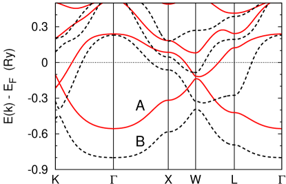
Figure 1: Band structures of pure metals A (full lines) and B (dashed lines) in a tight-binding $sp$ model on the fcc lattice. The horizontal dotted line denotes the position of the Fermi energy.

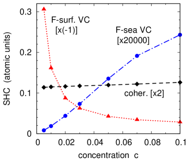
Figure 2: Three contributions to the spin Hall conductivity (SHC) for a tight-binding $sp$ model of a random fcc alloy A_1-cB_c as functions of the concentration $c$: the coherent term (diamonds), the vertex corrections to the Fermi surface term (triangles), and the vertex corrections to the Fermi sea term (circles). These contributions were rescaled by a factor of 2, $-1$, and 20000, respectively.

In this simple model of a random A_1-cB_c alloy, the fcc lattice parameter, the species-resolved LMTO potential parameters, and the alloy Fermi energy were kept fixed (independent on the concentration $c$). The resulting SHC contributions in the dilute alloy for $c\to 0$ are shown in Fig. 2; the SHC values are given in atomic units which is sufficient for the present purpose. One can see that the three contributions exhibit three different concentration trends for the vanishing impurity content: the coherent term ($\tilde{\sigma}^{(1)}_{xy,\mathrm{coh}}+\tilde{\sigma}^{(2)}_{xy,\mathrm{coh}}$) exhibits a finite nonzero limit, the Fermi surface vertex term ($\tilde{\sigma}^{(1)}_{xy,\mathrm{VC}}$) diverges with an inverse proportionality to $c$, and the Fermi sea vertex term ($\tilde{\sigma}^{(2)}_{xy,\mathrm{VC}}$) vanishes roughly linearly with $c$.

The divergence of the Fermi surface vertex term has been obtained and discussed by a number of authors Sinova et al. (2015); Gradhand et al. (2010); Lowitzer et al. (2011); this behavior of the extrinsic SHC has been ascribed to skew scattering. The weakly concentration dependent coherent term has also been found earlier Lowitzer et al. (2011); Chadova et al. (2015a). This trend justifies an identification of the coherent term with the intrinsic SHC of random alloys. Let us note however that the limit of the coherent SHC term for $c\to 0$ does not necessarily coincide with the SHC of the pure host metal A evaluated by using the Berry curvature approach from its band structure. This fact, ascribed to the coherent part of the side-jump contribution Sinova et al. (2015); Chadova et al. (2015b), can be explained by a sensitivity of the alloy selfenergy to the impurity B potential which affects the limiting value of the coherent SHC for $c\to 0$. A complete analysis of this point goes beyond the scope of this work.

The vertex corrections to the Fermi sea term have not been explicitly studied by other authors in the dilute limit. Since the same kernel $\Delta(z,z)$ is inverted in evaluation of Eq. (12) and in obtaining the energy derivative of the coherent potential function $\mathcal{P}^{\prime}(z)$, the revealed proportionality $\tilde{\sigma}^{(2)}_{xy,\mathrm{VC}}\sim c$ can be understood as a counterpart of the limiting behavior $\mathcal{P}^{\prime}(z)\to P^{\prime}_{\mathrm{A}}(z)$ for $c\to 0$, where $P_{\mathrm{A}}(z)$ denotes the potential function of the host metal A. Note however that the magnitude of the incoherent Fermi sea term is very small as compared to the other two terms (Fig. 2); since similarly tiny magnitudes were found for realistic alloy models even in concentrated regimes (Section III.2), a more detailed discussion of this term seems to be of little importance.

III.2 Random fcc Pt-based alloys

In this section, we address random fcc alloys of Pt with other heavy metals Au, Re, and Ta. For all systems, the average Wigner-Seitz (atomic sphere) radius of the alloy was set according to the Vegard’s law and the experimental values of the atomic sphere radii of the pure elements in their equilibrium structures. Local lattice relaxations were ignored which is acceptable because of similar sizes of all four elements.

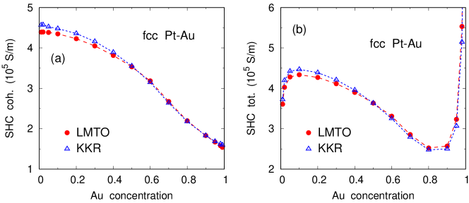
Figure 3: Comparison of the spin Hall conductivities (SHC) calculated in the TB-LMTO (solid circles) and KKR (open triangles) techniques for random fcc Pt-Au alloys: (a) the coherent part of the SHC and (b) the total SHC, both as functions of Au concentration. The results of the KKR method were taken from Ref. Obstbaum et al., 2016.

The total SHC and its intrinsic part for Pt-Au alloys are shown in Fig. 3; the TB-LMTO results are compared with those of the relativistic Korring-Kohn-Rostoker (KKR) method Obstbaum et al. (2016). One can see a very good agreement between both methods taking into account the different spin-current operators used: random, site-diagonal operators enter the KKR technique Lowitzer et al. (2010), whereas nonrandom, non-site-diagonal effective operators are employed in the present work (Section II.1). The intrinsic SHC decreases monotonically with increasing Au concentration (Fig. 3a); the extrinsic contribution modifies this trend significantly only near the limits of pure Pt and pure Au (Fig. 3b), where the divergent behavior dominates. For all concentrations, the vertex corrections to the Fermi sea term are about four orders of magnitude smaller than the SHC values in Fig. 3 and can thus be safely ignored. This feature has also been found in the KKR results Ködderitzsch et al. (2015).

The agreement between the results obtained by the TB-LMTO and the KKR techniques calls for a deeper theoretical explanation. Disregarding various technical details of both approaches, one finds that the most profound difference rests in the use of the usual, continuous coordinates in the KKR method and of the modified, steplike coordinates (constant inside each Wigner-Seitz cell) in the TB-LMTO method Turek et al. (2002). One can then prove that the two different current (velocity) operators lead to the same values of all elements of the standard conductivity tensor $\sigma_{\mu\nu}$. The proof employs relations between isothermic and adiabatic linear-response coefficients as well as properties of the current operator for systems in thermodynamic equilibrium, see Ref. r_s, for more details. We are unable to provide a similar proof for the spin-dependent conductivity tensor $\tilde{\sigma}_{\mu\nu}$; let us note that an equivalence of different torque operators for the Gilbert damping tensor in random ferromagnets has been shown elsewhere Turek et al. (2015); Drchal et al. (2017). Comparison of both approaches from a practical (numerical) point of view reveals essentially the same efficiency and accuracy in evaluation of the Fermi surface term of the conductivity tensors. The Fermi sea term, which involves energy derivatives of the Green’s functions, is treated by means of numerical derivatives in the KKR method Ködderitzsch et al. (2015), whereas analytical relations (owing to the parametrized potential functions and energy-independent structure constants) are used for these derivatives in the TB-LMTO method which seems advantageous for the computations.

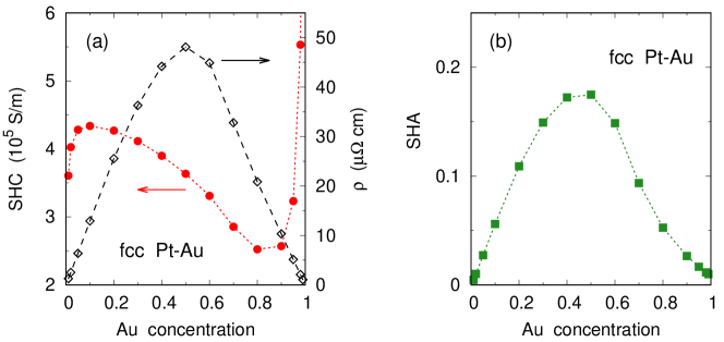
Figure 4: The calculated spin Hall conductivities (SHC), residual resistivities ($\rho$), and spin Hall angles (SHA) in random fcc Pt-Au alloys as functions of Au concentration: (a) SHC (solid circles, left scale) and $\rho$ (open diamonds, right scale) and (b) SHA (solid squares).

The calculated SHC values for Pt-Au alloys compare reasonably well to the measured ones in the entire concentration interval Obstbaum et al. (2016). Figure 4 displays the concentration trend of the SHC and of other transport quantities: the longitudinal resistivity $\rho$ and the SHA given by the product $\tilde{\sigma}_{xy}\rho$. One can see a maximum of $\rho$ for the equiconcentration alloy (Fig. 4a); a very similar concentration trend is obtained for the SHA with a maximum value slightly below 0.2 (Fig. 4b) which agrees again with the KKR results Obstbaum et al. (2016). This value is comparable with the top SHA values obtained for other alloys based on $5d$ transition metals Obstbaum et al. (2016); Fritz et al. (2018). Note however that the equiconcentration Pt-Au system is not thermodynamically stable at ambient temperatures according to its equilibrium phase diagram Massalski (1986) so that the measured samples are stabilized only by kinetic barriers. This fact calls for inspection of other alloy systems which might exhibit sizable SHA values for substitutional solid solutions that are equilibrium phases at low temperatures.

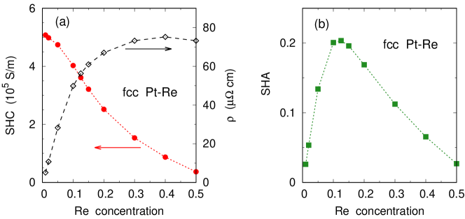
Figure 5: The same as Fig. 4 but for random fcc Pt-Re alloys.

In this work, we confined our interest to Pt-based alloys with fcc structure. The solubility limit of Re in fcc Pt is about 40 at.% Re Massalski (1986). The calculated values of SHC, $\rho$, and SHA are shown in Fig. 5. One can see a decreasing trend of the SHC due to alloying by Re, which is accompanied by a steep increase of the resistivity $\rho$ for small Re contents followed by a saturation of $\rho$ for higher Re concentrations (Fig. 5a). As a result of these trends, the SHA exhibits a maximum value of about 0.2 for Re content around 12 at.% Re (Fig. 5b). This composition falls safely inside the solubility interval of this alloy system and the predicted SHA value thus might deserve future experimental verification.

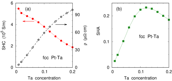
Figure 6: The same as Fig. 4 but for random fcc Pt-Ta alloys.

The phase diagram of the Pt-rich Pt-Ta system at ambient temperatures is not exactly known at present; extrapolations from higher temperatures indicate that the low-temperature solubility limit is about 15 at.% Ta Massalski (1986). The relevant collection of calculated SHC, $\rho$, and SHA is displayed in Fig. 6. One can observe opposite trends of SHC and $\rho$ due to alloying by Ta (Fig. 6a), in analogy with the Pt-Au (Fig. 4a) and Pt-Re (Fig. 5a) systems. The SHA exhibits a maximum again; the maximum SHA exceeds slightly the value 0.2 which is obtained for the alloy with about 12 at.% Ta (Fig. 6b). This composition should correspond to a thermodynamically stable primary solid solution.

The obtained maximum SHA values in all three studied Pt-based alloys result from a delicate competition between a reduction of SHC and an increase of $\rho$ due to alloying. Since these maximum values increase in sequence Pt-Au, Pt-Re, and Pt-Ta, one can ascribe a more important role to variations of $\rho$ which increases in the same sequence, as can be seen, e.g., by comparing the resistivities for alloys with 20 at.% of impurities. This importance of the longitudinal resistivity for large SHA values is in line with recent findings for the SHE in amorphous Hf-W alloys Fritz et al. (2018) as well as for SHE-based spin torques in multilayers with Pt-Al and Pt-Hf alloys Nguyen et al. (2016). Moreover, the resistivity variation is also responsible for the temperature dependence of the SHA both in bulk Pt-Au alloys Obstbaum et al. (2016) and in Pt layers adjacent to ferromagnetic Ni-Fe alloys Wang et al. (2016).

IV Conclusions

We have modified our recent theory of the relativistic electron transport in random alloys within the TB-LMTO-CPA method Turek et al. (2014) for the spin-dependent conductivity tensor. The derived formalism leads in general to three contributions to this tensor, namely (i) a coherent part, (ii) an incoherent part of the Fermi surface term, and (iii) an incoherent part of the Fermi sea term, which are all invariant with respect to the chosen TB-LMTO representation. The coherent part can be identified with an intrinsic contribution to the tensor, whereas the incoherent parts lead to an extrinsic contribution.

The developed theory is in principle applicable to a wide spectrum of phenomena involving spin-polarized currents induced by external electric fields encountered in systems with or without spontaneous magnetic moments. The performed analysis and calculations related to the spin Hall effect in nonmagnetic alloys revealed that the three contributions to the spin Hall conductivity exhibit three different concentration trends in the dilute limit and that the incoherent part of the Fermi sea term is negligibly small in the entire concentration interval. The obtained results for selected Pt-based binary alloys indicate that sizable values of the spin Hall angles can be obtained even for thermodynamically equilibrium primary solid solutions as an alternative to often studied metastable crystalline and amorphous alloys.

The approach worked out in this paper is not restricted only to the spin currents as observables; the derived formulas for the spin-dependent conductivity tensor represent essentially a complete result (within the TB-LMTO-CPA method) for the static linear response of any quantity to an external electric field. For this reason, a possible extension of the present theory towards a treatment of spin-orbit torques due to electric fields Manchon and Zhang (2009); Freimuth et al. (2014); Wimmer et al. (2016) seems (with the use of nonrandom effective torque operators Turek et al. (2015)) quite promising.

Appendix A Transformation invariance of the spin-dependent conductivity tensor

A.1 One-particle quantities

The study of the invariance of physical quantities with respect to the choice of the LMTO representation is based on relations for the coherent potential functions and the structure constants in two different representations, denoted by superscripts $\alpha$ and $\beta$:

$$\mathcal{P}^{\alpha}(z)=\left[1+\mathcal{P}^{\beta}(z)(\beta-\alpha)\right]^{-1}\mathcal{P}^{\beta}(z),\qquad S^{\alpha}=\left[1+S^{\beta}(\beta-\alpha)\right]^{-1}S^{\beta},$$ (13)

where the quantities $\alpha$ and $\beta$ in the brackets denote nonrandom site-diagonal matrices of the screening constants. Turek et al. (1997); Andersen et al. (1986) Let us introduce $\eta=\beta-\alpha$ and

$$M(z) = 1+\mathcal{P}^{\beta}(z)\eta,\qquad M^{\times}(z)=1+\eta\mathcal{P}^{\beta}(z),$$

$$K = 1+S^{\beta}\eta,\qquad K^{\times}=1+\eta S^{\beta},$$ (14)

and let us abbreviate $\bar{g}_{\pm}=\lim_{\epsilon\to 0^{+}}\bar{g}(E_{\mathrm{F}}\pm\mathrm{i}\epsilon)$ [and similarly for other energy dependent quantities, such as the coherent potential functions $\mathcal{P}(z)$, the site-diagonal matrices $M(z)$ and $M^{\times}(z)$, and the single-site T matrices $t_{\mathbf{R}}(z)$]. The transformation properties of the average auxiliary Green’s function $\bar{g}(z)$ can be summarized as

$$\bar{g}^{\alpha}(z) = M^{\times}(z)\bar{g}^{\beta}(z)M(z)-\eta M(z)=K^{\times}\bar{g}^{\beta}(z)K+K^{\times}\eta$$ (15)

$$= M^{\times}(z)\bar{g}^{\beta}(z)K=K^{\times}\bar{g}^{\beta}(z)M(z),$$

the energy derivative of $\bar{g}(z)$ transforms as

$$\bar{g}^{\prime,\alpha}(z)=K^{\times}\left[\bar{g}^{\prime,\beta}(z)M(z)+\bar{g}^{\beta}(z)M^{\prime}(z)\right]=K^{\times}\bar{g}^{\prime,\beta}(z)K,$$ (16)

and the transformation rule for the difference of two Green’s functions is

$$\bar{g}^{\alpha}_{+}-\bar{g}^{\alpha}_{-}=K^{\times}(\bar{g}^{\beta}_{+}-\bar{g}^{\beta}_{-})K.$$ (17)

The transformation properties of the effective velocities $\tilde{v}_{\mu}$ and $v_{\nu}$ are given by

$$\tilde{v}^{\alpha}_{\mu}=K^{-1}\tilde{v}^{\beta}_{\mu}(K^{\times})^{-1},\qquad v^{\alpha}_{\nu}=K^{-1}v^{\beta}_{\nu}(K^{\times})^{-1}.$$ (18)

All these transformation rules can be proved by procedures similar to those found in Refs. Turek et al., 2012; Andersen et al., 1986, taking into account also the spin independence of matrices $\alpha$, $\beta$, $S^{\alpha}$, $S^{\beta}$, and $K$.

The on-site blocks $M_{\mathbf{R}}(z)$ and $M^{\times}_{\mathbf{R}}(z)$ of the respective site-diagonal matrices $M(z)$ and $M^{\times}(z)$ enter also the transformation of the LMTO-CPA single-site T matrices $t_{\mathbf{R}}(z)$, namely,

$$t^{\beta}_{\mathbf{R}}(z)=M_{\mathbf{R}}(z)t^{\alpha}_{\mathbf{R}}(z)M^{\times}_{\mathbf{R}}(z),$$ (19)

see Refs. Turek et al., 1997, 2000 for more details.

A.2 Coherent contributions

The transformation of the coherent part of the Fermi surface term (5) is

$$\tilde{\sigma}^{(1),\alpha}_{\mu\nu,\mathrm{coh}}=\sigma_{0}\mathrm{Tr}\left\{\tilde{v}^{\alpha}_{\mu}(\bar{g}^{\alpha}_{+}-\bar{g}^{\alpha}_{-})v^{\alpha}_{\nu}\bar{g}^{\alpha}_{-}-\tilde{v}^{\alpha}_{\mu}\bar{g}^{\alpha}_{+}v^{\alpha}_{\nu}(\bar{g}^{\alpha}_{+}-\bar{g}^{\alpha}_{-})\right\}=\tilde{\sigma}^{(1),\beta}_{\mu\nu,\mathrm{coh}}+Z_{\mu\nu},$$ (20)

where the remainder can be written as

$$Z_{\mu\nu} = \sigma_{0}\mathrm{Tr}\left\{\tilde{v}^{\beta}_{\mu}(\bar{g}^{\beta}_{+}-\bar{g}^{\beta}_{-})v^{\beta}_{\nu}\eta K^{-1}-\tilde{v}^{\beta}_{\mu}\eta K^{-1}v^{\beta}_{\nu}(\bar{g}^{\beta}_{+}-\bar{g}^{\beta}_{-})\right\}$$ (21)

$$= \sigma_{0}\mathrm{Tr}\left\{Y_{\mu\nu}(\bar{g}^{\beta}_{+}-\bar{g}^{\beta}_{-})\right\},\qquad Y_{\mu\nu}=v^{\beta}_{\nu}\eta K^{-1}\tilde{v}^{\beta}_{\mu}-\tilde{v}^{\beta}_{\mu}\eta K^{-1}v^{\beta}_{\nu}.$$

This result proves that for metallic systems, the coherent part of $\tilde{\sigma}^{(1)}_{\mu\nu}$ depends on the particular LMTO representation.

The coherent part of the Fermi sea term (11) transforms as

$$\tilde{\sigma}^{(2),\alpha}_{\mu\nu,\mathrm{coh}}=\sigma_{0}\int_{C}\mathrm{d}z\mathrm{Tr}\left\{\tilde{v}^{\alpha}_{\mu}\bar{g}^{\prime,\alpha}(z)v^{\alpha}_{\nu}\bar{g}^{\alpha}(z)-\tilde{v}^{\alpha}_{\mu}\bar{g}^{\alpha}(z)v^{\alpha}_{\nu}\bar{g}^{\prime,\alpha}(z)\right\}=\tilde{\sigma}^{(2),\beta}_{\mu\nu,\mathrm{coh}}+R_{\mu\nu},$$ (22)

where the remainder is

$$R_{\mu\nu}=\sigma_{0}\int_{C}\mathrm{d}z\mathrm{Tr}\left\{\tilde{v}^{\beta}_{\mu}\bar{g}^{\prime,\beta}(z)v^{\beta}_{\nu}\eta K^{-1}-\tilde{v}^{\beta}_{\mu}\eta K^{-1}v^{\beta}_{\nu}\bar{g}^{\prime,\beta}(z)\right\}.$$ (23)

This remainder can be rewritten with the use of $\int_{C}\mathrm{d}z\bar{g}^{\prime,\beta}(z)=\bar{g}^{\beta}_{-}-\bar{g}^{\beta}_{+}$, which yields

$$R_{\mu\nu}=\sigma_{0}\mathrm{Tr}\left\{Y_{\mu\nu}(\bar{g}^{\beta}_{-}-\bar{g}^{\beta}_{+})\right\}=-Z_{\mu\nu}.$$ (24)

This result proves that the coherent part of $\tilde{\sigma}^{(2)}_{\mu\nu}$ depends on the choice of the LMTO representation as well, but the sum $\tilde{\sigma}^{(1)}_{\mu\nu,\mathrm{coh}}+\tilde{\sigma}^{(2)}_{\mu\nu,\mathrm{coh}}$, i.e., the total coherent part of $\tilde{\sigma}_{\mu\nu}$, is strictly invariant, as mentioned in Section II.3.

A.3 Incoherent part of the Fermi surface term

For the vertex corrections to the Fermi surface term (5), transformation properties are needed for all quantities entering the general expression for the LMTO vertex corrections Carva et al. (2006). The transformation rule for a two-particle quantity $\chi^{\Lambda_{1}\Lambda_{2}}_{\mathbf{R}_{1}\mathbf{R}_{2}}$ depending only on elements of the average auxiliary Green’s functions between different sites ($\mathbf{R}_{1}\neq\mathbf{R}_{2}$) and defined as

$$\chi^{\Lambda_{1}\Lambda_{2}}_{\mathbf{R}_{1}\mathbf{R}_{2}}=(1-\delta_{\mathbf{R}_{1}\mathbf{R}_{2}})(\bar{g}_{+})^{L_{1}L_{2}}_{\mathbf{R}_{1}\mathbf{R}_{2}}(\bar{g}_{-})^{L^{\prime}_{2}L^{\prime}_{1}}_{\mathbf{R}_{2}\mathbf{R}_{1}},$$ (25)

where $\Lambda_{1}=(L_{1},L^{\prime}_{1})$, $\Lambda_{2}=(L_{2},L^{\prime}_{2})$, is given with the help of Eq. (15) by

$$\chi^{\alpha}=\Pi\chi^{\beta}\tilde{\Pi},$$ (26)

where we introduced site-diagonal quantities $\Pi^{\Lambda_{1}\Lambda_{2}}_{\mathbf{R}_{1}\mathbf{R}_{2}}=\delta_{\mathbf{R}_{1}\mathbf{R}_{2}}\Pi^{\Lambda_{1}\Lambda_{2}}_{\mathbf{R}_{1}}$ and $\tilde{\Pi}^{\Lambda_{1}\Lambda_{2}}_{\mathbf{R}_{1}\mathbf{R}_{2}}=\delta_{\mathbf{R}_{1}\mathbf{R}_{2}}\tilde{\Pi}^{\Lambda_{1}\Lambda_{2}}_{\mathbf{R}_{1}}$, where

$$\Pi^{\Lambda_{1}\Lambda_{2}}_{\mathbf{R}}=\left(M^{\times}_{+,\mathbf{R}}\right)^{L_{1}L_{2}}\left(M_{-,\mathbf{R}}\right)^{L^{\prime}_{2}L^{\prime}_{1}},\qquad\tilde{\Pi}^{\Lambda_{1}\Lambda_{2}}_{\mathbf{R}}=\left(M_{+,\mathbf{R}}\right)^{L_{1}L_{2}}\left(M^{\times}_{-,\mathbf{R}}\right)^{L^{\prime}_{2}L^{\prime}_{1}}.$$ (27)

The site-diagonal quantity $w^{\Lambda_{1}\Lambda_{2}}_{\mathbf{R}_{1}\mathbf{R}_{2}}=\delta_{\mathbf{R}_{1}\mathbf{R}_{2}}w^{\Lambda_{1}\Lambda_{2}}_{\mathbf{R}_{1}}$, where $w^{\Lambda_{1}\Lambda_{2}}_{\mathbf{R}}=\left\langle t^{L_{1}L_{2}}_{+,\mathbf{R}}t^{L^{\prime}_{2}L^{\prime}_{1}}_{-,\mathbf{R}}\right\rangle$, satisfies the transformation relation

$$w^{\beta}=\tilde{\Pi}w^{\alpha}\Pi,$$ (28)

which follows from Eq. (19). As a consequence of the rules (26) and (28), the matrix $\Delta=w^{-1}-\chi$ and its inverse transform as

$$\Delta^{\alpha}=\Pi\Delta^{\beta}\tilde{\Pi},\qquad(\Delta^{\alpha})^{-1}=\tilde{\Pi}^{-1}(\Delta^{\beta})^{-1}\Pi^{-1}.$$ (29)

For transformations of the on-site blocks $(\bar{g}_{+}v_{\nu}\bar{g}_{-})^{L_{1}L^{\prime}_{1}}_{\mathbf{R}\mathbf{R}}\equiv(\bar{g}_{+}v_{\nu}\bar{g}_{-})^{\Lambda_{1}}_{\mathbf{R}}$ and $(\bar{g}_{-}\tilde{v}_{\mu}\bar{g}_{+})^{L^{\prime}_{1}L_{1}}_{\mathbf{R}\mathbf{R}}\equiv(\bar{g}_{-}\tilde{v}_{\mu}\bar{g}_{+})^{\tilde{\Lambda}_{1}}_{\mathbf{R}}$, one can use relations (15) and (18) for the Green’s functions and velocities, respectively. The result is

$$(\bar{g}^{\alpha}_{+}v^{\alpha}_{\nu}\bar{g}^{\alpha}_{-})^{\Lambda_{1}}_{\mathbf{R}}=\sum_{\Lambda_{2}}\Pi^{\Lambda_{1}\Lambda_{2}}_{\mathbf{R}}(\bar{g}^{\beta}_{+}v^{\beta}_{\nu}\bar{g}^{\beta}_{-})^{\Lambda_{2}}_{\mathbf{R}},\qquad(\bar{g}^{\alpha}_{-}\tilde{v}^{\alpha}_{\mu}\bar{g}^{\alpha}_{+})^{\tilde{\Lambda}_{1}}_{\mathbf{R}}=\sum_{\Lambda_{2}}(\bar{g}^{\beta}_{-}\tilde{v}^{\beta}_{\mu}\bar{g}^{\beta}_{+})^{\tilde{\Lambda}_{2}}_{\mathbf{R}}\tilde{\Pi}^{\Lambda_{2}\Lambda_{1}}_{\mathbf{R}},$$ (30)

where the symbols $\tilde{\Lambda}_{1}=(L^{\prime}_{1},L_{1})$ and $\tilde{\Lambda}_{2}=(L^{\prime}_{2},L_{2})$ denote indices transposed to $\Lambda_{1}=(L_{1},L^{\prime}_{1})$ and $\Lambda_{2}=(L_{2},L^{\prime}_{2})$, respectively.

The transformation of the vertex corrections to the Fermi surface term (5) is now straightforward Carva et al. (2006). The identity (8) yields $\mathrm{Tr}\left\langle\tilde{v}_{\mu}g_{+}v_{\nu}g_{+}\right\rangle_{\mathrm{VC}}=\mathrm{Tr}\left\langle\tilde{v}_{\mu}g_{-}v_{\nu}g_{-}\right\rangle_{\mathrm{VC}}=0$, so that $\tilde{\sigma}^{(1)}_{\mu\nu,\mathrm{VC}}=2\sigma_{0}\mathrm{Tr}\left\langle\tilde{v}_{\mu}g_{+}v_{\nu}g_{-}\right\rangle_{\mathrm{VC}}$ and

$$\tilde{\sigma}^{(1),\alpha}_{\mu\nu,\mathrm{VC}}=2\sigma_{0}\sum_{\mathbf{R}_{1}\Lambda_{1}}\sum_{\mathbf{R}_{2}\Lambda_{2}}(\bar{g}^{\alpha}_{-}\tilde{v}^{\alpha}_{\mu}\bar{g}^{\alpha}_{+})^{\tilde{\Lambda}_{1}}_{\mathbf{R}_{1}}\left[(\Delta^{\alpha})^{-1}\right]^{\Lambda_{1}\Lambda_{2}}_{\mathbf{R}_{1}\mathbf{R}_{2}}(\bar{g}^{\alpha}_{+}v^{\alpha}_{\nu}\bar{g}^{\alpha}_{-})^{\Lambda_{2}}_{\mathbf{R}_{2}}.$$ (31)

The last relation combined with the transformations (29) and (30) leads to the invariance of the vertex corrections to the Fermi surface term, $\tilde{\sigma}^{(1),\alpha}_{\mu\nu,\mathrm{VC}}=\tilde{\sigma}^{(1),\beta}_{\mu\nu,\mathrm{VC}}$.

A.4 Incoherent part of the Fermi sea term

The vertex corrections to the Fermi sea term (12) can be written as $(-2\sigma_{0})\int_{C}\mathrm{d}zQ(z)$, where the quantity $Q(z)$ in the LMTO representation $\alpha$ is given explicitly by

$$Q^{\alpha}=\sum_{\mathbf{R}_{1}\Lambda_{1}}\sum_{\mathbf{R}_{2}\Lambda_{2}}(\bar{g}^{\alpha}\tilde{v}^{\alpha}_{\mu}\bar{g}^{\alpha})^{\tilde{\Lambda}_{1}}_{\mathbf{R}_{1}}\left[(\Delta^{\alpha})^{-1}\right]^{\Lambda_{1}\Lambda_{2}}_{\mathbf{R}_{1}\mathbf{R}_{2}}(\bar{g}^{\alpha}v^{\alpha}_{\nu}\bar{g}^{\prime,\alpha})^{\Lambda_{2}}_{\mathbf{R}_{2}},$$ (32)

where all energy arguments (equal to $z$) have been omitted, see Eq. (12), where $\Lambda_{1}=(L_{1},L^{\prime}_{1})$, $\Lambda_{2}=(L_{2},L^{\prime}_{2})$, $\tilde{\Lambda}_{1}=(L^{\prime}_{1},L_{1})$, and $\tilde{\Lambda}_{2}=(L^{\prime}_{2},L_{2})$, and where the same identifications have been done as before, namely, $(\bar{g}v_{\nu}\bar{g}^{\prime})^{L_{1}L^{\prime}_{1}}_{\mathbf{R}\mathbf{R}}\equiv(\bar{g}v_{\nu}\bar{g}^{\prime})^{\Lambda_{1}}_{\mathbf{R}}$ and $(\bar{g}\tilde{v}_{\mu}\bar{g})^{L^{\prime}_{1}L_{1}}_{\mathbf{R}\mathbf{R}}\equiv(\bar{g}\tilde{v}_{\mu}\bar{g})^{\tilde{\Lambda}_{1}}_{\mathbf{R}}$.

The transformation of individual factors in Eq. (32) is similar to the previous case of the Fermi surface term. In particular, the transformation rules for $\Delta^{\alpha}$ and its inverse, Eq. (29), remain valid but with the quantities $\Pi_{\mathbf{R}}$ and $\tilde{\Pi}_{\mathbf{R}}$ defined as

$$\Pi^{\Lambda_{1}\Lambda_{2}}_{\mathbf{R}}=\left(M^{\times}_{\mathbf{R}}\right)^{L_{1}L_{2}}\left(M_{\mathbf{R}}\right)^{L^{\prime}_{2}L^{\prime}_{1}},\qquad\tilde{\Pi}^{\Lambda_{1}\Lambda_{2}}_{\mathbf{R}}=\left(M_{\mathbf{R}}\right)^{L_{1}L_{2}}\left(M^{\times}_{\mathbf{R}}\right)^{L^{\prime}_{2}L^{\prime}_{1}},$$ (33)

where the matrices $M_{\mathbf{R}}$ and $M^{\times}_{\mathbf{R}}$ are taken with the same (omitted) energy argument $z$. The transformation of $(\bar{g}\tilde{v}_{\mu}\bar{g})^{\tilde{\Lambda}_{1}}_{\mathbf{R}}$ is similar to Eq. (30), namely,

$$(\bar{g}^{\alpha}\tilde{v}^{\alpha}_{\mu}\bar{g}^{\alpha})^{\tilde{\Lambda}_{1}}_{\mathbf{R}}=\sum_{\Lambda_{2}}(\bar{g}^{\beta}\tilde{v}^{\beta}_{\mu}\bar{g}^{\beta})^{\tilde{\Lambda}_{2}}_{\mathbf{R}}\tilde{\Pi}^{\Lambda_{2}\Lambda_{1}}_{\mathbf{R}},$$ (34)

while the transformation of $(\bar{g}v_{\nu}\bar{g}^{\prime})^{\Lambda_{1}}_{\mathbf{R}}$ is based on relation (16), which leads to

$$(\bar{g}^{\alpha}v^{\alpha}_{\nu}\bar{g}^{\prime,\alpha})^{L_{1}L^{\prime}_{1}}_{\mathbf{R}\mathbf{R}}=(M^{\times}\bar{g}^{\beta}v^{\beta}_{\nu}\bar{g}^{\prime,\beta}M)^{L_{1}L^{\prime}_{1}}_{\mathbf{R}\mathbf{R}}+(M^{\times}\bar{g}^{\beta}v^{\beta}_{\nu}\bar{g}^{\beta}M^{\prime})^{L_{1}L^{\prime}_{1}}_{\mathbf{R}\mathbf{R}},$$ (35)

where the second term on the r.h.s. vanishes due to the identity (8) and due to the site-diagonal nature of matrices $M$, $M^{\times}$ and $M^{\prime}$. This yields

$$(\bar{g}^{\alpha}v^{\alpha}_{\nu}\bar{g}^{\prime,\alpha})^{\Lambda_{1}}_{\mathbf{R}}=\sum_{\Lambda_{2}}\Pi^{\Lambda_{1}\Lambda_{2}}_{\mathbf{R}}(\bar{g}^{\beta}v^{\beta}_{\nu}\bar{g}^{\prime,\beta})^{\Lambda_{2}}_{\mathbf{R}},$$ (36)

again in analogy with Eq. (30). The use of the rules (29), (34) and (36) in Eq. (32) leads to $Q^{\alpha}(z)=Q^{\beta}(z)$, which proves the transformation invariance of the vertex corrections to the Fermi sea term, $\tilde{\sigma}^{(2),\alpha}_{\mu\nu,\mathrm{VC}}=\tilde{\sigma}^{(2),\beta}_{\mu\nu,\mathrm{VC}}$.

This completes the proof of the invariance of the total spin-dependent conductivity tensor $\tilde{\sigma}_{\mu\nu}$ (4) with respect to the choice of the LMTO representation.

Appendix B (Supplemental material) Equivalence of the KKR and TB-LMTO conductivity tensors

In this part, we sketch a proof of equivalence of the conductivity tensors based (i) on the usual, continuous coordinates used in the KKR method, and (ii) on the modified, piecewise constant coordinates employed in the TB-LMTO technique. Turek et al. (2002) In both cases we consider the same one-particle Hamiltonian $H$ and denote its retarded and advanced Green’s functions as $G_{\pm}(E)=(E\pm i0-H)^{-1}$, where $E$ is a real energy variable.

Basic definitions and relations.

Let us start with a few basic definitions and relations. If $A$ denotes a Hermitian operator representing a one-particle observable quantity, its thermodynamic equilibrium average value $Q(A)$ can be expressed as

$$Q(A)=\frac{i}{2\pi}\int\mathrm{d}Ef(E)\mathrm{Tr}\{AD(E)\},$$ (37)

where we abbreviated

$$D(E)=G_{+}(E)-G_{-}(E)$$ (38)

and where $f(E)$ denotes the Fermi-Dirac function. Let $B$ denote another one-particle Hermitian operator which, added as a small perturbation to the unperturbed Hamiltonian $H$, defines a new thermodynamic equilibrium (with the same Fermi-Dirac function) of the system and let us assume that this perturbation leaves the operator $A$ unchanged. The corresponding first-order changes in the Green’s functions are $\delta G_{\pm}(E)=G_{\pm}(E)BG_{\pm}(E)$ which induces a change in the average value of $A$ equal to $\delta Q(A)=R(A,B)$, where

$$R(A,B)=\frac{i}{2\pi}\int\mathrm{d}Ef(E)\mathrm{Tr}\{AG_{+}(E)BG_{+}(E)-AG_{-}(E)BG_{-}(E)\}$$ (39)

defines the relevant isothermic linear-response coefficient (susceptibility). An obvious symmetry relation

$$R(A,B)=R(B,A)$$ (40)

is valid owing to the cyclic property of the trace. For the adiabatic linear response, we introduce a symbol

$$C(A_{1},A_{2})=\frac{1}{2\pi}\int\mathrm{d}Ef(E)\mathrm{Tr}\{A_{1}D(E)A_{2}G^{2}_{-}(E)-A_{1}G^{2}_{+}(E)A_{2}D(E)\},$$ (41)

where $A_{1}$ and $A_{2}$ are Hermitian operators. If these operators are identified with two components of the velocity (current) operator, then $C(A_{1},A_{2})$ defines (apart from a prefactor) an element of the Kubo conductivity tensor as given by the formula of Bastin et al. Bastin et al. (1971) Note that for energy derivative of the Green’s functions, the well-known relation $G^{\prime}_{\pm}(E)=-G^{2}_{\pm}(E)$ has been used.

Further relations.

We prove now several useful relations among the introduced quantities $Q(A)$, $R(A,B)$ and $C(A_{1},A_{2})$. Let us assume that the operator $A_{2}$ is a time derivative of an operator $B_{2}$, so that ($\hbar=1$)

$$A_{2}=-i[B_{2},H],$$ (42)

and that $B_{2}$ can be considered as a perturbation with the property mentioned before Eq. (39). Then one can write

$$A_{2}=iB_{2}(E-H)-i(E-H)B_{2}$$ (43)

in Eq. (41) and one can use relations

$$(E-H)G_{\pm}(E)=G_{\pm}(E)(E-H)=1$$ (44)

and

$$(E-H)D(E)=D(E)(E-H)=0,$$ (45)

which follow from the definitions of the Green’s functions and from Eq. (38). The trace in Eq. (41) can be then simplified as

$$\mathrm{Tr}\{A_{1}D(E)A_{2}G^{2}_{-}(E)-A_{1}G^{2}_{+}(E)A_{2}D(E)\}$$ (46)

$$= i\,\mathrm{Tr}\{A_{1}D(E)B_{2}(E-H)G^{2}_{-}(E)-A_{1}D(E)(E-H)B_{2}G^{2}_{-}(E)$$

$$\quad{}-A_{1}G^{2}_{+}(E)B_{2}(E-H)D(E)+A_{1}G^{2}_{+}(E)(E-H)B_{2}D(E)\}$$

$$= i\,\mathrm{Tr}\{A_{1}D(E)B_{2}G_{-}(E)+A_{1}G_{+}(E)B_{2}D(E)\}$$

$$= i\,\mathrm{Tr}\{A_{1}G_{+}(E)B_{2}G_{+}(E)-A_{1}G_{-}(E)B_{2}G_{-}(E)\},$$

which yields a relation

$$C(A_{1},A_{2})=R(A_{1},B_{2}).$$ (47)

Similarly, if $A_{1}$ in Eq. (41) is a time derivative of an operator $B_{1}$ with the property mentioned before Eq. (39),

$$A_{1}=-i[B_{1},H],$$ (48)

one can prove that

$$C(A_{1},A_{2})=-R(B_{1},A_{2}).$$ (49)

Finally, one can prove in a similar way that if both operators $A_{1}$ and $A_{2}$ in Eq. (41) can be written according to Eq. (48) and Eq. (42), respectively, then

$$C(A_{1},A_{2})=Q(i[B_{1},B_{2}]).$$ (50)

The proof of equivalence of both conductivity tensors employs the relations (47, 49, 50).

Proof of equivalence.

We denote the operator of the usual, continuous coordinate as $r_{\mu}$ ($\mu=x,y,z$) and that of the modified coordinate, constant in each Wigner-Seitz cell, as $r^{0}_{\mu}$; their difference is denoted as $\xi_{\mu}$, so that

$$r_{\mu}=r^{0}_{\mu}+\xi_{\mu}.$$ (51)

The time derivatives of the coordinate operators $r_{\mu}$, $r^{0}_{\mu}$ and $\xi_{\mu}$ due to the Hamiltonian $H$ are denoted as $V_{\mu}$, $V^{0}_{\mu}$ and $U_{\mu}$, respectively. These velocity operators satisfy the obvious relation

$$V_{\mu}=V^{0}_{\mu}+U_{\mu}.$$ (52)

It should be noted that only the difference coordinate $\xi_{\mu}$, which is bounded due to a finite size of the Wigner-Seitz cells, can be used as a perturbation that defines a new thermodynamic equilibrium; the other two coordinates ($r_{\mu}$, $r^{0}_{\mu}$), which are unbounded in infinite solids, do not possess this property. This means that only the relation

$$U_{\mu}=-i[\xi_{\mu},H]$$ (53)

can be used as a special case of relations (42) and (48).

The elements of the KKR conductivity tensor can be (apart from a prefactor) identified with $C(V_{\mu},V_{\nu})$ while their TB-LMTO counterparts are given by $C(V^{0}_{\mu},V^{0}_{\nu})$. We have then

$$C(V_{\mu},V_{\nu})=C(V^{0}_{\mu},V^{0}_{\nu})+C(V^{0}_{\mu},U_{\nu})+C(U_{\mu},V^{0}_{\nu})+C(U_{\mu},U_{\nu})$$ (54)

as a simple consequence of Eq. (41) and Eq. (52). The last term in Eq. (54) vanishes due to Eq. (53) and the rule (50),

$$C(U_{\mu},U_{\nu})=Q(i[\xi_{\mu},\xi_{\nu}])=0,$$ (55)

since $[\xi_{\mu},\xi_{\nu}]=0$ (the coordinate operators commute mutually). Before the treatment of the other terms in Eq. (54), let us discuss the quantity $C(V_{\mu},U_{\nu})$. It holds

$$C(V_{\mu},U_{\nu})=R(V_{\mu},\xi_{\nu})$$ (56)

as a consequence of Eq. (53) and Eq. (47). Let us prove that the r.h.s. of Eq. (56) vanishes. We start with a general relation

$$Q(V_{\mu})=0,$$ (57)

which is nothing but an exact vanishing of the average value of the total electric current in thermodynamic equilibrium. If we add the operator $\xi_{\nu}$ as a perturbation to the Hamiltonian $H$ (which defines a new equilibrium of the system) and if we take into account that this perturbation does not modify the velocity operator $V_{\mu}$ (since $[r_{\mu},\xi_{\nu}]=0$), we obtain the same exact vanishing of the average value of the total electric current also for the perturbed system. This means that the corresponding linear-response coefficient (39) vanishes as well, hence

$$R(V_{\mu},\xi_{\nu})=0.$$ (58)

Combination of this result with Eq. (56) and Eq. (52) yields

$$C(V_{\mu},U_{\nu})=C(V^{0}_{\mu},U_{\nu})+C(U_{\mu},U_{\nu})=0.$$ (59)

By using the previous relation (55), we get

$$C(V^{0}_{\mu},U_{\nu})=0,$$ (60)

so that the second term on the r.h.s. of Eq. (54) vanishes. Let us consider finally the term $C(U_{\mu},V^{0}_{\nu})$. With application of Eq. (53), Eq. (49), Eq. (40), Eq. (47), and Eq. (60), we get

$$C(U_{\mu},V^{0}_{\nu})=-R(\xi_{\mu},V^{0}_{\nu})=-R(V^{0}_{\nu},\xi_{\mu})=-C(V^{0}_{\nu},U_{\mu})=0.$$ (61)

The last three terms on the r.h.s. of Eq. (54) thus vanish, see Eqs. (55, 60, 61), which yields

$$C(V_{\mu},V_{\nu})=C(V^{0}_{\mu},V^{0}_{\nu}).$$ (62)

This completes the proof of equivalence of both conductivity tensors.

References

- Maekawa et al. (2012) S. Maekawa, S. O. Valenzuela, E. Saitoh, and T. Kimura, eds., Spin Current (Oxford University Press, 2012).
- Tsymbal and Žutić (2012) E. Y. Tsymbal and I. Žutić, eds., Handbook of Spin Transport and Magnetism (CRC Press, Boca Raton, 2012).
- Sinova et al. (2015) J. Sinova, S. O. Valenzuela, J. Wunderlich, C. H. Back, and T. Jungwirth, Rev. Mod. Phys. 87, 1213 (2015).
- Hirsch (1999) J. E. Hirsch, Phys. Rev. Lett. 83, 1834 (1999).
- Guo et al. (2008) G. Y. Guo, S. Murakami, T.-W. Chen, and N. Nagaosa, Phys. Rev. Lett. 100, 096401 (2008).
- Freimuth et al. (2010) F. Freimuth, S. Blügel, and Y. Mokrousov, Phys. Rev. Lett. 105, 246602 (2010).
- Gradhand et al. (2010) M. Gradhand, D. V. Fedorov, P. Zahn, and I. Mertig, Phys. Rev. Lett. 104, 186403 (2010).
- Lowitzer et al. (2011) S. Lowitzer, M. Gradhand, D. Ködderitzsch, D. V. Fedorov, I. Mertig, and H. Ebert, Phys. Rev. Lett. 106, 056601 (2011).
- Nagaosa et al. (2010) N. Nagaosa, J. Sinova, S. Onoda, A. H. MacDonald, and N. P. Ong, Rev. Mod. Phys. 82, 1539 (2010).
- Zimmermann et al. (2014) B. Zimmermann, K. Chadova, D. Ködderitzsch, S. Blügel, H. Ebert, D. V. Fedorov, N. H. Long, P. Mavropoulos, I. Mertig, Y. Mokrousov, and M. Gradhand, Phys. Rev. B 90, 220403(R) (2014).
- Chadova et al. (2015a) K. Chadova, S. Wimmer, H. Ebert, and D. Ködderitzsch, Phys. Rev. B 92, 235142 (2015a).
- Obstbaum et al. (2016) M. Obstbaum, M. Decker, A. K. Greitner, M. Haertinger, T. N. G. Meier, M. Kronseder, K. Chadova, S. Wimmer, D. Ködderitzsch, H. Ebert, and C. H. Back, Phys. Rev. Lett. 117, 167204 (2016).
- Wang et al. (2016) L. Wang, R. J. H. Wesselink, Y. Liu, Z. Yuan, K. Xia, and P. J. Kelly, Phys. Rev. Lett. 116, 196602 (2016).
- Borge and Tokatly (2017) J. Borge and I. V. Tokatly, Phys. Rev. B 96, 115445 (2017).
- Amin et al. (2018) V. P. Amin, J. Zemen, and M. D. Stiles, Phys. Rev. Lett. 121, 136805 (2018).
- Li et al. (2019) S. Li, K. Shen, and K. Xia, Phys. Rev. B 99, 134427 (2019).
- Wesselink et al. (2019) R. J. H. Wesselink, K. Gupta, Z. Yuan, and P. J. Kelly, Phys. Rev. B 99, 144409 (2019).
- Wimmer et al. (2015) S. Wimmer, M. Seemann, K. Chadova, D. Ködderitzsch, and H. Ebert, Phys. Rev. B 92, 041101(R) (2015).
- Ralph and Stiles (2008) D. C. Ralph and M. D. Stiles, J. Magn. Magn. Mater. 320, 1190 (2008).
- Lowitzer et al. (2010) S. Lowitzer, D. Ködderitzsch, and H. Ebert, Phys. Rev. B 82, 140402(R) (2010).
- Zhang et al. (2017) Y. Zhang, Y. Sun, H. Yang, J. Železný, S. P. P. Parkin, C. Felser, and B. Yan, Phys. Rev. B 95, 075128 (2017).
- Zhang et al. (2018) Y. Zhang, J. Železný, Y. Sun, J. van den Brink, and B. Yan, New J. Phys. 20, 073028 (2018).
- Wang et al. (2006) Y. Wang, K. Xia, Z.-B. Su, and Z. Ma, Phys. Rev. Lett. 96, 066601 (2006).
- Shi et al. (2006) J. Shi, P. Zhang, D. Xiao, and Q. Niu, Phys. Rev. Lett. 96, 076604 (2006).
- Turek et al. (2002) I. Turek, J. Kudrnovský, V. Drchal, L. Szunyogh, and P. Weinberger, Phys. Rev. B 65, 125101 (2002).
- Soven (1967) P. Soven, Phys. Rev. 156, 809 (1967).
- Velický (1969) B. Velický, Phys. Rev. 184, 614 (1969).
- Turek et al. (2012) I. Turek, J. Kudrnovský, and V. Drchal, Phys. Rev. B 86, 014405 (2012).
- Turek et al. (2014) I. Turek, J. Kudrnovský, and V. Drchal, Phys. Rev. B 89, 064405 (2014).
- Kubo (1957) R. Kubo, J. Phys. Soc. Jpn. 12, 570 (1957).
- Bastin et al. (1971) A. Bastin, C. Lewiner, O. Betbeder-Matibet, and P. Nozieres, J. Phys. Chem. Solids 32, 1811 (1971).
- Andersen (1975) O. K. Andersen, Phys. Rev. B 12, 3060 (1975).
- Andersen and Jepsen (1984) O. K. Andersen and O. Jepsen, Phys. Rev. Lett. 53, 2571 (1984).
- Crépieux and Bruno (2001) A. Crépieux and P. Bruno, Phys. Rev. B 64, 014416 (2001).
- Carva et al. (2006) K. Carva, I. Turek, J. Kudrnovský, and O. Bengone, Phys. Rev. B 73, 144421 (2006).
- Manchon and Zhang (2009) A. Manchon and S. Zhang, Phys. Rev. B 79, 094422 (2009).
- Freimuth et al. (2014) F. Freimuth, S. Blügel, and Y. Mokrousov, Phys. Rev. B 90, 174423 (2014).
- Wimmer et al. (2016) S. Wimmer, K. Chadova, M. Seemann, D. Ködderitzsch, and H. Ebert, Phys. Rev. B 94, 054415 (2016).
- Andersen et al. (1986) O. K. Andersen, Z. Pawlowska, and O. Jepsen, Phys. Rev. B 34, 5253 (1986).
- Turek et al. (2015) I. Turek, J. Kudrnovský, and V. Drchal, Phys. Rev. B 92, 214407 (2015).
- Chadova et al. (2015b) K. Chadova, D. V. Fedorov, C. Herschbach, M. Gradhand, I. Mertig, D. Ködderitzsch, and H. Ebert, Phys. Rev. B 92, 045120 (2015b).
- Hyodo et al. (2016) K. Hyodo, A. Sakuma, and Y. Kota, Phys. Rev. B 94, 104404 (2016).
- Kudrnovský and Drchal (1990) J. Kudrnovský and V. Drchal, Phys. Rev. B 41, 7515 (1990).
- Turek et al. (1997) I. Turek, V. Drchal, J. Kudrnovský, M. Šob, and P. Weinberger, Electronic Structure of Disordered Alloys, Surfaces and Interfaces (Kluwer, Boston, 1997).
- Ködderitzsch et al. (2015) D. Ködderitzsch, K. Chadova, and H. Ebert, Phys. Rev. B 92, 184415 (2015).
- (46) See Supplemental Material (Appendix B) for a proof of equivalence of the KKR and TB-LMTO conductivity tensors.
- Drchal et al. (2017) V. Drchal, I. Turek, and J. Kudrnovský, J. Supercond. Nov. Magn. 30, 1669 (2017).
- Fritz et al. (2018) K. Fritz, S. Wimmer, H. Ebert, and M. Meinert, Phys. Rev. B 98, 094433 (2018).
- Massalski (1986) T. B. Massalski, ed., Binary Alloy Phase Diagrams (American Society for Metals, Metals Park, Ohio, 1986).
- Nguyen et al. (2016) M.-H. Nguyen, M. Zhao, D. C. Ralph, and R. A. Buhrman, Appl. Phys. Lett. 108, 242407 (2016).
- Turek et al. (2000) I. Turek, J. Kudrnovský, and V. Drchal, in Electronic Structure and Physical Properties of Solids, Lecture Notes in Physics, Vol. 535, edited by H. Dreyssé (Springer, Berlin, 2000) p. 349.