A high-magnetic-field radio pulsar survey with Swift/XRT

Abstract

We present the X-ray survey results of high-magnetic-field radio pulsars (high-B PSRs) with Swift/XRT. X-ray observations of the rotation-powered pulsars with the dipole magnetic field ${\it B_{\rm d}}$ near the quantum critical field ${\it B_{\rm q}}=4.4\times 10^{13}$ G is of great importance for understanding the transition between the rotation-powered pulsars and the magnetars, because there are a few objects that have magnetar-like properties. Out of the 27 high-B PSRs that are in the ATNF pulsar catalogue but have not been reported or have no effective upper-limits in the X-ray bands, we analyze the Swift/XRT data for 21 objects, where 6 objects are newly observed and 15 objects are taken from the archival data. As a result, we have new $3\sigma$ upper-limits for all the 21 objects. Since the upper-limits are tight, we conclude that we do not find any magnetar-like high-B PSRs such as PSR J1819$-$1458. The probability of the high X-ray efficiency in the high-B PSRs is obtained to be $11\%-29\%$. Combining the previous observations, we discuss which parameter causes magnetar-like properties. It may be suggested that the magnetar-like properties appear only when ${\it B_{\rm d}}\gtrsim 10^{13.5}$ G for the radio pulsar population. This is true even if the radio-quiet high-B RPP are included.

1 Introduction

Isolated neutron stars are known to have two major populations according to the source of their energy. One is the rotation-powered pulsars (RPPs) (for a review, see Beskin et al. 2015). These are mostly observed as radio pulsars (PSRs) or gamma-ray pulsars. The other population is the high magnetic pulsars, called magnetars for short (for a review, see Kaspi & Beloborodov 2017 and Turolla et al. 2015). These are characterised by frequent bursting activity, lasting from a fraction of a second to several tens of seconds, and by high X-ray luminosity larger than the spin-down luminosity $L_{\rm rot}$.

What causes this distinctive manifestation of neutron stars as either RPPs or magnetars is not yet understood. The dipole component of the neutron star magnetic field can be inferred from the spin period $P$ and its time derivative $\dot{P}$ as $B_{d}\approx 1.1\times 10^{12}(P/1\mbox{s})^{1/2}(\dot{P}/10^{-15})^{1/2}$ G. Since most magnetars have a very strong dipole magnetic field exceeding the quantum critical field ${B_{\rm q}}=m^{2}c^{3}/\hbar e=4.4\times 10^{13}$ G, it was thought that the strength of the dipole field is the key parameter. However, discovery of the “weak-field magnetar” SGR 0418$+$5729, whose dipole field $B_{d}\sim 6.1\times 10^{12}$ G is much less than $B_{\rm q}$ (Esposito et al., 2010; Rea et al., 2010, 2013), indicates that dipole field strength is not always essential. Theoretically, the toroidal field is proposed to play an essential role for magnetar activity (Pons & Perna, 2011). The toroidal field together with the poloidal field evolves interactively from very large values $\gtrsim 10^{14}$ G at birth to their present state, and is expected to form multi-pole fields that cause bursts and extra heating.

A small group of RPPs called high-magnetic-field RPPs (high-B RPPs), some of which are radio-quiet pulsars, may be key to understand the strong magnetic fields of the neutron stars. The inferred dipole magnetic field of high-B RPPs is similar to or larger than ${B_{\rm q}}$. These are interestingly symbiotic objects in the sense that they exhibit both RPP-like and magnetar-like features. In fact, high-B RPPs generally behave very much like RPPs, but two recently exhibited magnetar-like outbursts (see Archibald et al. 2016 regarding an outburst from PSR J1119$-$6127, Gavriil et al. 2008 for PSR J1846$-$258), and three are known to have high X-ray luminosity as compared with the typical luminosity of RPPs, $\sim 10^{-3}L_{\rm rot}$ (Seward & Wang, 1988; Becker & Truemper, 1997; Becker et al., 2009; Kargaltsev et al., 2012; Shibata et al., 2016).

To provide better and possibly new insights for the symbiosis seen in high-B RPPs, we intend to sample more X-ray counterparts of high-B RPPs. Previously, some high-B RPPs were observed intensively (Olausen et al., 2013), and an X-ray counterpart survey with Chandra and XMM-Newton was done by Prinz & Becker (2015). It is notable here that the magnetospheric emission of RPPs declines rapidly with spin-down, so that thermal radiation, which may be due to strong multi-pole magnetic fields, is easier to be detected in objects with $L_{\rm rot}\lesssim 10^{35}\mbox{erg s${}^{-1}$}$. However, the survey for such objects with relatively small spin-down luminosity is not complete. Toward a more complete survey, in this paper we report the first results of a systematic survey for X-ray counterparts using archival data and additional observations with the X-ray Telescope (XRT; Burrows et al. 2005) onboard the Neil Gehrels Swift Observatory (Gehrels et al., 2004).

2 Data Preparation and Observation

Using the Australia Telescope National Facility (ATNF) pulsar catalogue (Manchester et al., 2005), we made a list of high-B PSRs with inferred dipole magnetic fields above $10^{13}$ G. Since our targets are PSRs, we excluded magnetars, X-ray isolated neutron star (XINS), radio-quiet pulsars, and binary members from the ATNF catalogue using type codes AXP, XINS, NRAD and BINARY . A total of 56 objects were selected. After a literature search, 27 objects were found to have no X-ray detections or no effective upper-limits less than $10^{35}$ erg s^-1. We searched Swift/XRT archival data that include the radio positions of these 27 high-B PSRs within 12 arcmin from the Swift pointing position in photon counting (PC) mode. As a result, available data were found for 16 of the 27 objects, as listed in Table 1. There were no X-ray observations for the remaining 11 objects.

We attempted additional Swift observations for the remaining objects. We selected objects that can be detected at 10 sigma or more with 2 ks exposure time if their luminosities are as large as that of PSR J1819$-$1458 ($1.75\times 10^{33}$ erg s^-1; McLaughlin et al. 2007), which is considered to be a typical value of magnetic origin for the thermal radiation seen in high-B PSRs. As a result, we selected 5 objects. The observation parameters for these objects are given in Table 2. Note that we performed a second observation for PSR J1851$+$0118, since it gave 4$\sigma$ detection in the first analysis of the archival data (Table 2).

We performed the analysis for the 21 pulsars. The locations in the $P-\dot{P}$ diagram of those pulsars are shown in Figure 1, in which we overlay other neutron star populations.

Swift/XRT data were processed using HEASOFT v6.24, xrtpipeline v0.13.4 and the Calibration Database files of version 20160731. Standard level-2 cleaned events files were generated for further analysis. We did not use data that suffered from stray light.

Table 1: Summary of the Swift/XRT X-ray archival data used.

PSR name	Datea	number of the data	XRT exposure
	(start-end)		ks
J0534$-$6703	2011 Oct 20 $-$ 2015 Sep 01	4	3.23
J1107$-$6143	2010 Aug 04 $-$ 2011 Jan 27	3	4.36
J1307$-$6318	2011 Feb 18 $-$ 2011 Sep 30	2	1.20
J1632$-$4818	2012 Jun 13 $-$ 2011 Sep 30	1	0.48
J1713$-$3844	2012 Aug 11 $-$ 2011 Sep 30	1	0.57
J1746$-$2850	2011 Aug 18 $-$ 2016 Jun 06	921b	866b
J1755$-$2521	2012 Sep 07 $-$ 2016 Jun 06	1	0.31
J1822$-$1252	2012 Oct 25 $-$ 2012 Nov 01	4	2.10
J1830$-$1135	2012 Nov 04 $-$ 2012 Nov 01	1	0.50
J1851$+$0118	2012 Nov 20 $-$ 2012 Feb 20	3	1.15
J1854$+$0306	2013 Mar 25 $-$ 2012 Feb 20	1	0.51
J1855$+$0527	2011 Nov 16 $-$ 2013 Mar 07	3	1.50
J1858$+$0241	2013 Mar 27 $-$ 2013 Mar 24	7	4.58
J1901$+$0413	2012 Feb 18 $-$ 2013 Mar 24	1	0.46
J1905$+$0616	2012 Nov 29 $-$ 2012 Feb 18	2	1.39
J1924$+$1631	2012 Apr 10 $-$ 2012 Apr 10	2	1.08
aWhen a PSR has multiple data, the start date of the first observation and the end date of the finial overvation are given.
b The values are for the analysis of the 0.3$-$1.5 keV and the 0.3$-$3.0 keV bands, but for the analysis of the 0.3$-$10 keV band, the number of data is 920 and the total exposure time is 865 ks.

Table 2: Summary of our X-ray observations with Swift/XRT.

PSR name	Date	ObsID	XRT exposure	off-axis
	(start-end)		(ks)	(arcmin)
B052$5+$21	2016 Aug 20 $-$ 2016 Aug 20	00034683001	1.80	1.34
B1727$-$47	2016 May 22 $-$ 2016 May 23	00034538001	1.77	0.60
J0140$+$5622a	2016 Jun 03 $-$ 2016 Jun 04	00034537001	2.89	1.82
J1558$-$5756	2016 May 11 $-$ 2016 May 11	00034536001	0.07	4.58
	2016 May 21 $-$ 2016 May 21	00034536002	0.46	1.44
	2016 Jun 16 $-$ 2016 Jun 16	00034536003	1.20	0.95
J1840$-$0840	2016 May 21 $-$ 2016 May 21	00034540001	0.27	0.76
	2016 Jun 13 $-$ 2016 Jun 13	00034540002	1.78	1.34
J1851$+$0118b	2018 Feb 28 $-$ 2018 Feb 28	00010585001	5.06	2.53
a J0140$+$5622 is cited in the ATNF pulsar catalogue as J0139$+$5621.
b We performed a 2nd observation of PSR J1851$+$0118 because it gave a 4$\sigma$ detection in the first analysis of the archival data.

Figure 1: $P-\dot{P}$ diagram for our samples, indicated by filled black circles with other populations. Dots indicate RPPs listed in the ATNF pulsar catalogue. $\times$ symbols and asterisks indicate XINSs (Viganò et al., 2013) and magnetars (Olausen & Kaspi, 2014), respectively.

3 Analysis and Results

For the X-ray counterpart search, significance against the background depends on the choice of energy band. We suppose three types of spectral models in order to optimise the energy range for count extraction. The first type is a low-temperature high-B PSR model, which is a single blackbody model with $kT=0.15$ keV. The second is a high-temperature magnetar-like high-B PSR model, which is a single blackbody model with $kT=0.3$ keV. The final type is an ordinary PSR model, which is a single power law model with a photon index of $1.5$. The assumed temperature in the first model is the average value of the high-B PSRs PSR J0726$+$2612 (Speagle et al., 2011), PSR J1819$-$1458 (McLaughlin et al., 2007), PSR J1718$-$3718 (Zhu et al., 2011), and PSR J1119$-$6127 (Ng et al., 2012). The temperature in the second model is that of PSR J1734$-$3333 (Olausen et al., 2013), which has the highest temperature among detected high-B PSRs. This value also sometimes appears in persistent magnetars. For the photon index in the third model, we used the average of the high-B PSRs PSR J1930$+$1852 (Lu et al., 2007), PSR J1124$-$5916 (Hughes et al., 2001), PSR B1509$-$58 (Kargaltsev et al., 2008), and PSR J1119$-$6127 (Ng et al., 2012).

Given a fake spectrum for each of the three types of objects and a background spectrum, we calculated S/N ratio as a function of the energy bands. As a result, the optimized energy bands were determined to be the $0.3-1.5$ keV band for the low-temperature high-B PSR model, the $0.3-3.0$ keV band for the high-temperature magnetar-like high-B PSR model, and the $0.3-10$ keV band for the ordinary PSRs model. The source region was assumed to be circular with a 20-pixel radius (47.1 arcsec), which corresponds to the 90% encircled energy radius at 1.5 keV. We obtained the background spectrum from six source-free circular regions of 20-pixels in radius, where we took data from an 8.7 ks observation of XINS RXJ0720.4$-$3125 (ObsId 00050200005), 26 ks observation of the same object (ObsId 00050203001) and the 13 ks observation of XINS RXJ1856.5$-$3754 (ObsId 00051950025). We changed the normalization as $1\times 10^{-4}$, $1\times 10^{-5}$ and $1\times 10^{-6}$ for the blackbody model with $kT=0.15$ keV, and the optimal energy bands were hardly changed.

In this study, we analysed data for these three energy bands. We extracted source counts from each dataset using a circular region of 20 pixels in radius centred on the radio position. The background region was not uniquely determined for every observation, because the observations were not targeted to the pulsar and there were some number of bad pixels. The background region is a set of 6 circular regions with radii of 20 pixels, selected from 24 candidate regions to minimize bad pixels and defects in the field of view with “SAOImage DS9” and “Funtools”.

Using the correction factor yielded by xrtmkarf for the exposure, vignetting, and bad columns and pixels, we obtained corrected source and background counts. When an object had multiple observations, we summed the corrected source and background counts, and calculated the total exposure for each object.

We evaluated the significance of source counts for every three bands according to Poisson statistics (Gehrels, 1986). We found no detections with significance larger than $3\sigma$. We then calculated the $3\sigma$ upper limits using Poisson statistics (Gehrels, 1986). The obtained upper-limit count rates are given in Table 3. Unabsorbed flux in the $0.3-10$ keV band were also found using the PIMMS (Portable Interactive Multi-Mission Simulator) tool, where the spectral model is the corresponding one and the hydrogen column density ${\it N_{\rm H}}$ is calculated from the dispersion measure by the empirical relation in He et al. (2013). We calculated the intrinsic X-ray luminosities in Table 3 using distances taken from the ATNF catalogue.

We estimated systematic uncertainty caused by the selected background using unbiased variances of the background counts. As a result, average systematic uncertainties at the $1\sigma$ confidence level for each band were 7.6%, 8.0%, and 11.7% of the $3\sigma$ confidence limit. The upper limits in terms of the X-ray luminosity ${\it L_{\rm x}}$ are plotted against the spin-down luminosity in Figure 2. One can see that some of the upper limits are less than the luminosity of the persistent emission of the magnetars and PSR J1819$-$1458 having the highest X-ray efficiency in the high-B PSRs.

In Figure 3, we compare the upper limits of the ordinary PSR model with the $1.0-10$ keV X-ray luminosity at the burst phase of the transient magnetars given in Table 6 of Enoto et al. (2017). Our upper limits are smaller than the burst phase luminosity of Swift J1822.3$-$1606, except for seven upper limits. Therefore, we can see that they did not magnetically explode during Swift observations.

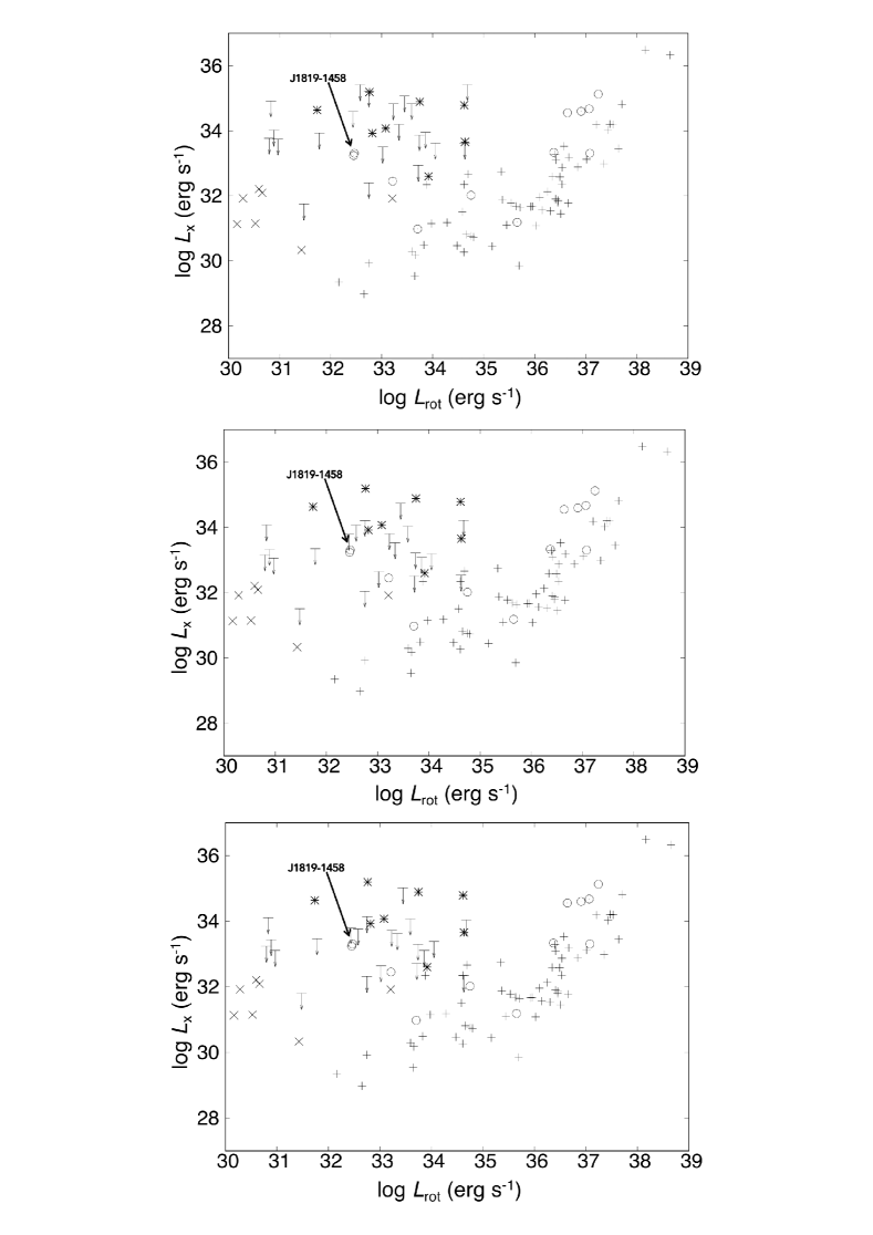
Figure 2: The 3$\sigma$ upper limits are shown as arrows in the ${\rm log}~{}{\it L_{\rm x}}-{\rm log}~{}{\it L_{\rm rot}}$ diagram for the present objects with other populations in the $0.3-10$ keV band. White circles indicate high-B PSRs detected in previous studies. The symbol "$+$" indicates PSRs for which data were taken from Table LABEL:PlotData. Crosses and asterisks indicate XINSs (Viganò et al., 2013) and magnetars (Olausen & Kaspi, 2014) (see Table LABEL:PlotData), respectively. The top, middle, and bottom panels show results from the low-temperature high-B PSR model, the high-temperature magnetar-like high-B PSR model, and the ordinary PSRs model, respectively.

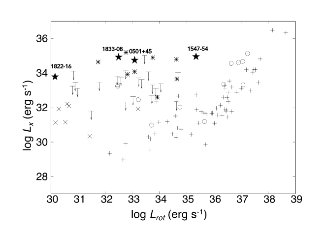
Figure 3: ${\rm Log}~{}{\it L_{\rm x}}-{\rm log}~{}{\it L_{\rm rot}}$ diagram of the power law model in the $0.3-10$ keV band for transient magnetars. Star symbols indicate the soft-component X-ray luminosity at burst phase in the $1-10$ keV band of transient magnetars given in Table 6 of Enoto et al. (2017). Other symbols are the same as in Figure 2. Our upper limits are smaller than the burst-phase luminosity of Swift J1822.3$-$1606, except for seven upper limits.

Table 3: Summary of X-ray survey of RPPs by Swift/XRT

Result of the 0.3-1.5 keV band

Result of the 0.3-3.0 keV band

Result of the 0.3-10 keV band

PSR name

Exp.a

${\rm log}$ ${\it B_{\rm d}}$

${\rm log}$ ${\it P}$

${\rm log}$ ${\it P_{\rm dot}}$

Dist.

${\it N_{\rm H}}$

log ${\it L_{\rm rot}}$

cps

$F^{\rm unabs}_{\rm x}$

${\rm log}$ ${\it L^{\rm unabs}_{\rm x}}$

cps

$F^{\rm unabs}_{\rm x}$

${\rm log}$ ${\it L^{\rm unabs}_{\rm x}}$

cps

$F^{\rm unabs}_{\rm x}$

${\rm log}$ ${\it L^{\rm unabs}_{\rm x}}$

ks

G

s

s/s

kpc

pc ${\rm cm^{-2}}$

erg/s

counts/s

erg s-1cm-2

erg/s

counts/s

erg s-1cm-2

erg/s

counts/s

erg s-1cm-2

erg/s

B0525+21

1.81

13.09

0.57

-13.40

1.22

1.53$\times 10^{21}$

31.48

<5.34$\times 10^{-3}$

<3.13$\times 10^{-13}$

<31.75

<5.34$\times 10^{-3}$

<1.81$\times 10^{-13}$

<31.51

<5.78$\times 10^{-3}$

<3.53$\times 10^{-13}$

<31.80

B1727-47

1.78

13.07

-0.08

-12.79

5.57

3.70$\times 10^{21}$

34.05

<8.11$\times 10^{-3}$

<1.12$\times 10^{-12}$

<33.62

<8.36$\times 10^{-3}$

<4.19$\times 10^{-13}$

<33.19

<8.58$\times 10^{-3}$

<6.55$\times 10^{-13}$

<33.38

J0140+5622b

2.90

13.08

0.25

-13.10

2.41

3.06$\times 10^{21}$

32.75

<3.31$\times 10^{-3}$

<3.65$\times 10^{-13}$

<32.40

<3.57$\times 10^{-3}$

<1.61$\times 10^{-13}$

<32.05

<4.17$\times 10^{-3}$

<3.01$\times 10^{-13}$

<32.32

J0534-6703

3.24

13.45

0.26

-12.37

49.70

2.84$\times 10^{21}$

33.45

<3.94$\times 10^{-3}$

<4.02$\times 10^{-13}$

<35.07

<4.33$\times 10^{-3}$

<1.89$\times 10^{-13}$

<34.74

<5.07$\times 10^{-3}$

<3.59$\times 10^{-13}$

<35.02

J1107-6143

4.38

13.23

0.26

-12.81

2.94

1.22$\times 10^{22}$

33.02

<2.97$\times 10^{-3}$

<3.05$\times 10^{-12}$

<33.50

<3.34$\times 10^{-3}$

<4.36$\times 10^{-13}$

<32.65

<3.65$\times 10^{-3}$

<4.23$\times 10^{-13}$

<32.64

J1307-6318

1.21

13.02

0.70

-13.68

10.78

1.12$\times 10^{22}$

30.83

<6.98$\times 10^{-3}$

<5.99$\times 10^{-12}$

<34.92

<7.30$\times 10^{-3}$

<8.73$\times 10^{-13}$

<34.08

<8.20$\times 10^{-3}$

<9.21$\times 10^{-13}$

<34.11

J1558-5756

1.73

13.17

0.05

-12.73

3.32

3.83$\times 10^{21}$

33.72

<4.54$\times 10^{-3}$

<6.55$\times 10^{-13}$

<32.94

<4.80$\times 10^{-3}$

<2.46$\times 10^{-13}$

<32.51

<5.03$\times 10^{-3}$

<3.88$\times 10^{-13}$

<32.71

J1632-4818

0.48

13.37

-0.09

-12.19

5.31

2.27$\times 10^{22}$

34.68

<1.47$\times 10^{-2}$

<7.91$\times 10^{-11}$

<35.42

<1.73$\times 10^{-2}$

<4.95$\times 10^{-12}$

<34.22

<2.13$\times 10^{-2}$

<3.26$\times 10^{-12}$

<34.04

J1713-3844

0.57

13.23

0.20

-12.75

4.43

1.63$\times 10^{22}$

33.23

<1.39$\times 10^{-2}$

<2.88$\times 10^{-11}$

<34.83

<1.52$\times 10^{-2}$

<2.78$\times 10^{-12}$

<33.81

<1.72$\times 10^{-2}$

<2.26$\times 10^{-12}$

<33.72

J1746-2850c

870.0d

13.59

1.08

0.00

5.61

2.89$\times 10^{22}$

34.63

<9.10$\times 10^{-5}$

<1.11$\times 10^{-12}$

<33.62

<2.25$\times 10^{-4}$

<9.29$\times 10^{-14}$

<32.54

<3.36$\times 10^{-4}$

<5.79$\times 10^{-14}$

<32.34

J1755-2521

0.31

13.02

0.07

-13.04

3.44

7.56$\times 10^{21}$

33.34

<2.80$\times 10^{-2}$

<1.12$\times 10^{-11}$

<34.20

<2.92$\times 10^{-2}$

<2.41$\times 10^{-12}$

<33.53

<3.03$\times 10^{-2}$

<2.93$\times 10^{-12}$

<33.62

J1822-1252

2.11

13.13

0.32

-13.07

6.38

2.78$\times 10^{22}$

32.58

<5.15$\times 10^{-3}$

<5.41$\times 10^{-11}$

<35.42

<6.23$\times 10^{-3}$

<2.41$\times 10^{-12}$

<34.07

<7.09$\times 10^{-3}$

<1.20$\times 10^{-12}$

<33.76

J1830-1135

0.50

13.24

0.79

-13.32

3.76

7.71$\times 10^{21}$

30.89

<1.50$\times 10^{-2}$

<6.21$\times 10^{-12}$

<34.02

<1.50$\times 10^{-2}$

<1.27$\times 10^{-12}$

<33.33

<1.68$\times 10^{-2}$

<1.63$\times 10^{-12}$

<33.44

J1840-0840

2.06

13.06

0.73

-13.63

5.10

8.16$\times 10^{21}$

30.80

<4.20$\times 10^{-3}$

<1.92$\times 10^{-12}$

<33.77

<5.30$\times 10^{-3}$

<4.69$\times 10^{-13}$

<33.16

<5.64$\times 10^{-3}$

<5.60$\times 10^{-13}$

<33.24

J1851+0118

4.63

13.05

-0.04

-12.86

5.64

1.25$\times 10^{22}$

33.86

<2.14$\times 10^{-3}$

<2.35$\times 10^{-12}$

<33.95

<2.37$\times 10^{-3}$

<3.19$\times 10^{-13}$

<33.08

<2.88$\times 10^{-3}$

<3.38$\times 10^{-13}$

<33.11

J1854+0306

0.51

13.42

0.66

-12.84

4.49

5.77$\times 10^{21}$

31.78

<1.39$\times 10^{-2}$

<3.55$\times 10^{-12}$

<33.93

<1.39$\times 10^{-2}$

<9.29$\times 10^{-13}$

<33.35

<1.39$\times 10^{-2}$

<1.22$\times 10^{-12}$

<33.47

J1855+0527

1.51

13.29

0.14

-12.57

11.70

1.09$\times 10^{22}$

33.59

<5.22$\times 10^{-3}$

<4.18$\times 10^{-12}$

<34.83

<5.74$\times 10^{-3}$

<6.64$\times 10^{-13}$

<34.04

<6.48$\times 10^{-3}$

<7.18$\times 10^{-13}$

<34.07

J1858+0241

4.60

13.03

0.67

-13.61

5.15

1.01$\times 10^{22}$

30.97

<2.56$\times 10^{-3}$

<1.76$\times 10^{-12}$

<33.74

<3.35$\times 10^{-3}$

<3.61$\times 10^{-13}$

<33.06

<3.79$\times 10^{-3}$

<4.08$\times 10^{-13}$

<33.11

J1901+0413

0.47

13.28

0.43

-12.88

5.34

1.06$\times 10^{22}$

32.44

<1.51$\times 10^{-2}$

<1.15$\times 10^{-11}$

<34.59

<1.62$\times 10^{-2}$

<1.82$\times 10^{-12}$

<33.79

<1.73$\times 10^{-2}$

<1.90$\times 10^{-12}$

<33.81

J1905+0616

1.39

13.07

0.00

-12.87

4.95

7.68$\times 10^{21}$

33.74

<6.23$\times 10^{-3}$

<2.56$\times 10^{-12}$

<33.87

<6.77$\times 10^{-3}$

<5.68$\times 10^{-13}$

<33.22

<7.03$\times 10^{-3}$

<6.82$\times 10^{-13}$

<33.30

J1924+1631

1.08

13.52

0.47

-12.44

10.19

1.56$\times 10^{22}$

32.75

<7.29$\times 10^{-3}$

<1.34$\times 10^{-11}$

<35.22

<7.66$\times 10^{-3}$

<1.32$\times 10^{-12}$

<34.21

<8.70$\times 10^{-3}$

<1.12$\times 10^{-12}$

<34.14

Notes. All upper-limits are $3\sigma$ upper-limits.

The X-ray flux and the X-ray luminosity is the unabsorbed X-ray flux and the intrinsic X-ray luminosity in the 0.3$-$10 keV band.

a The total exposure time after the data reduction.

b J0140+5622 is cited in the ATNF pulsar catalogue as J0139+5621.

c Result with Chandra is given by Dexter et al. (2017).

d When the 0.3-10 keV band is analysed, this value is 869.00.

4 Discussion

In this section, we discuss properties of the high-B RPPs. In subsection 4.1 we discuss dependence on the dipole magnetic field, and in subsection 4.2 we estimate a fraction of the high-efficiency high-B PSRs in the PSR population.

4.1 Dependence of dipole magnetic field on flux

We found that magnetar-like properties appear only when ${\it B_{\rm d}}\gtrsim 10^{13.5}$ G for the radio pulsar population. This is true even if the radio-quiet high-B RPP are included. To see this, we compiled the detected X-ray flux of high-B RPPs and ordinary PSRs in the literature. For the dataset of ordinary PSRs, we restrict ourselves to pulsars with “rotational energy flux,” defined as ${\it F_{\rm rot}}={\it L_{\rm rot}}/4\pi D^{2}$ larger than $1\times 10^{-11}$ erg s^-1 cm^-2, because these would show detectable flux if they have an excess as compared with typical ordinary pulsars. We also prepared data for magnetars and XINSs given in Olausen & Kaspi (2014) and Viganò et al. (2013). The $0.3$-$10$ keV luminosities are given in Table LABEL:PlotData. We also utilise upper-limit data satisfying the conditions that the distance is less than 4 kpc and the exposure time is longer than 1 ks. There are 12 upper limits in total, of which 4 are our results and 8 are taken from previous reports. We do not use data where too few spectral parameters are given for the band conversion.

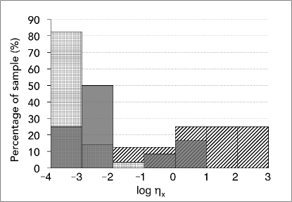
Figure 4: Efficiency distributions for RPPs (checked bars), magnetars (striped bars), and high-B RPPs (dark grey bars). The data are based on Table LABEL:PlotData.

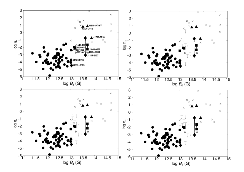
Figure 5: Inferred dipole magnetic field versus X-ray efficiency. Black filled circles indicate PSRs with ${\it B_{\rm d}}<10^{13.5}$ G, and triangles, rectangles, diamonds and grey circles indicate high-B RPPs, defined as ${\it B_{\rm d}}\geq 10^{13.5}$ G, where the different symbols correspond to the different manifestations, namely, triangular ones are high X-ray efficiency pulsars, rectangular ones are soft-gamma-ray pulsars, diamond ones are the gamma-ray pulsars observed with Fermi/LAT and grey circular ones are low X-ray efficiency and a simple blackbody pulsars. Crosses and asterisks indicate XINSs and magnetars, respectively. Data are based on Table LABEL:PlotData. Top-right, bottom-left, and bottom-right panels are the same as the top-left panel, except that the upper limits on 4 of our results and 8 previous results are overlaid with arrows. The 8 previous results are given in Prinz & Becker (2015), Pivovaroff et al. (2000), and Uchiyama et al. (2011). Top-right, bottom-left, and bottom-right panels indicate results from the blackbody model with $kT=0.15$ keV, that with $kT=0.3$ keV, and the power law model with photon index $1.5$.

First, we plot the distribution of the X-ray efficiency $\eta_{x}={\it L_{\rm x}}/{\it L_{\rm rot}}$ in the $0.3$-$10$ keV band for the three classes, high-B RPPs, ordinary PSRs, and magnetars in Figure 4. The efficiencies of the magnetars (striped histograms in Figure 4) are more than 0.01%, while those of the ordinary PSRs (checked) are less than $0.1\%$. The high-B RPPs (dark grey) seem to exhibit a bimodal distribution: one is a high-efficiency group where $\eta_{x}>0.1\%$ and the other is a low-efficiency group where $\eta_{x}<0.01\%$.

It was suggested in Olausen et al. (2010) that X-ray luminosity or efficiency weakly correlates with the dipole field ${\it B_{\rm d}}$ across wider neutron star populations. We provide a ${\rm log}~{}\eta_{\rm x}$ versus ${\rm log}~{}{\it B_{\rm d}}$ plot in Figure 5. In the panels of Figure 5, the distribution of ordinary radio pulsars (filled circles) and high-B RPPs (filled triangles, rectangles, diamonds, and grey circles) seems to show a stepwise structure in $\eta_{\rm x}$ at ${\it B_{\rm d}}\sim 10^{13.5}$ G.

On the right side, where ${\it B_{\rm d}}>10^{13.5}$ G, all high-B RPPs show some features of magnetars, such as high efficiency or burst activity, except for PSR J1734$-$3333 (discussed below). On the left side, where ${\it B_{\rm d}}<10^{13.5}$ G, these high-B RPPs behave like ordinary pulsars where $\eta_{\rm x}$ is low.

For the case of ${\it B_{\rm d}}>10^{13.5}$ G, PSR J1718$-$3718, PSR J0726$-$2612, and PSR J1819$-$1458 show high X-ray efficiency at the relatively high temperature of $0.08$-$0.18$ keV. The X-ray pulse fractions of PSR J1718$-$3718 and PSR J1819$-$1458 are $52\pm 13\%$ in the $0.8$-$2.0$ keV band and $34\pm 6\%$ in the $0.3$-$5$ keV band (Zhu et al., 2011; McLaughlin et al., 2007). As for PSR J0726$-$2612, the semi-amplitude is given to be $27\pm 5\%$ in the $0.32$-$1.1$ keV band (Speagle et al., 2011). These properties are an indication of magnetic activity on the surface. Burst activity was found in PSR J1846$-$0258 and PSR J1119$-$6127. The former shows a magnetar-like outburst in 2006. In quiescence, it is a soft-gamma-ray pulsar with pulsar wind nebula. The efficiency is ${\rm log}~{}\eta_{\rm x}=-2.52$ in the quiescent state and becomes ${\rm log}~{}\eta_{\rm x}=-1.73$ at the burst state (Ng et al., 2008). The latter also shows a magnetar-like outburst in 2016, and observations by Fermi/LAT suggest it to be an ordinary RPP. The efficiency is ${\rm log}~{}\eta_{\rm x}=-3.11$ in quiescence and became ${\rm log}~{}\eta_{\rm x}=-0.82$ during the burst (Ng et al., 2012; Archibald et al., 2016).

Members in the low-field side, ${\it B_{\rm d}}<10^{13.5}$ G, manifest themselves differently. (1) PSR B1509$-$58, PSR J1930$+$1852, and PSR J1640$-$4631 are referred to as soft-gamma-ray pulsars, indicated by rectangles in Figure 5 (Kuiper & Hermsen, 2015), (2) PSR J0007$+$7303 and PSR J1124$-$5916 are classified in the gamma-ray pulsars observed with Fermi/LAT, indicated by diamonds (Abdo et al., 2013), and (3) PSR B1916$+$14, indicated by the filled grey circle, shows low efficiency and a simple blackbody spectrum (Olausen et al., 2013; Zhu et al., 2009).

The meaning of these apparent differences is not clear. However, they would not be related to the strength of the dipole fields, because (1) the dipole field strength of the soft gamma-ray pulsars are widely distributed, from $7.5\times 10^{11}$ G to $4.9\times 10^{13}$ G, (2) Fermi/LAT pulsars are very common in RPPs with various field strengths, and (3) thermally dominant X-ray radiation is also common in middle-aged RPPs.

In summary, the three highly efficient and two bursting high-B RPPs all have larger dipole fields than a threshold at ${\it B_{\rm d}}\sim 10^{13.5}$ G. This argument may be strengthened if we add the high-B RPPs that have tight upper limits. We plotted the upper limits with arrows in the top-right, bottom-left, and bottom-right panels in Figure 5. Some upper limits confirm that objects are definitely not as X-ray efficient as PSR J1718$-$3718 and rather like a normal PSR. There are 9 such objects.

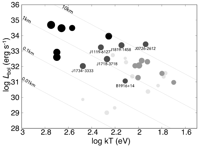
Figure 6: ${\rm Log}~{}{\it kT}$-${\rm log}~{}{\it L_{\rm bol}}$ diagram, where $kT$ and ${\it L_{\rm bol}}$ are the blackbody temperature and the bolometric luminosity from Table 4 and Table LABEL:PlotData. The light grey, grey, dark grey, and black circles indicate PSRs, XINSs, high-B RPPs, and magnetars, respectively. Circle sizes indicate strength of the dipole magnetic field. Lines show the radiative radius calculated as $\sqrt{{{\it L_{\rm x}}/4\pi\sigma T^{4}}}$.

Table 4: PSRs and high-B RPPs with blackbody components.

PSR name	type	${\it B_{\rm d}}$	Dist.	Temp.	modela	component	log${\it L_{\rm bol}}$	log${\it L_{\rm rot}}$	Reference
		G	kpc	keV			erg/s	erg/s
B0656+14	B0	4.66e+12	0.29	0.059	PL+BB+BB	Blackbody 1	31.57	34.58	Bîrzan et al. (2016)
B0656+14	B0	4.66e+12	0.29	0.113	PL+BB+BB	Blackbody 2	31.36	34.58	Bîrzan et al. (2016)
B0833-45	B0	3.39e+12	0.28	0.128	PL+BB	Blackbody	32.28	36.84	Pavlov et al. (2001)
B1055-52	B0	1.09e+12	0.09	0.068	PL+BB+BB	Blackbody 1	30.76	34.48	Posselt et al. (2015)
B1055-52	B0	1.09e+12	0.09	0.16	PL+BB+BB	Blackbody 2	29.33	34.48	Posselt et al. (2015)
B1706-44	B0	3.13e+12	2.60	0.166	PL+BB	Blackbody	32.74	36.53	Romani et al. (2005)
B1822-09	B0	6.44e+12	0.30	0.083	BB+BB	Blackbody 1	30.38	33.66	Hermsen et al. (2017)
B1822-09	B0	6.44e+12	0.30	0.187	BB+BB	Blackbody 2	29.01	33.66	Hermsen et al. (2017)
B1916+14	B0	1.60e+13	1.30	0.13	BB	Blackbody	31.06	33.71	Zhu et al. (2009)
B1929+10	B0	5.19e+11	0.31	0.30	PL+BB	Blackbody	29.87	33.60	Misanovic et al. (2008)
B1951+32	B0	4.86e+11	3.00	0.13	PL+BB	Blackbody	32.53	36.57	Li et al. (2005)
J1741-2054	B0	2.69e+12	0.30	0.061	PL+BB	Blackbody	31.35	33.98	Marelli et al. (2014)
J0726-2612	HB	3.21e+13	2.90	0.087	BB	Blackbody	33.44	32.45	Speagle et al. (2011)
J1119-6127	HB	4.10e+13	8.40	0.21	PL+BB	Blackbody	33.24	36.37	Ng et al. (2012)
J1718-3718	HB	7.46e+13	3.92	0.186	BB	Blackbody	32.48	33.22	Zhu et al. (2011)
J1734-3333	HB	5.24e+13	4.46	0.30	BB	Blackbody	32.03	34.75	Olausen et al. (2013)
J1819-1458	HB	5.01e+13	3.30	0.14	BB	Blackbody	33.38	32.47	McLaughlin et al. (2007)
J0501+4516	Mag	1.85E+14	2.20	0.5	PL+BB	Blackbody	32.92	33.08	Camero et al. (2014)
J1050-5953	Mag	5.02E+14	9.00	0.56	PL+BB	Blackbody	34.69	33.75	Tam et al. (2008)
J1622-4950	Mag	2.75E+14	5.57	0.5	BB	Blackbody	32.60	33.92	Anderson et al. (2012)
J1708-4008	Mag	4.70E+14	3.80	0.456	PL+BB	Blackbody	34.48	32.76	Rea et al. (2007)
J1809-1943	Mag	1.27E+14	3.60	0.28	BB	Blackbody	33.96	32.82	Gotthelf et al. (2004)
J2301+5852	Mag	5.81E+13	3.30	0.37	PL+BB	Blackbody	34.49	31.74	Zhu et al. (2008)
aPL and BB indicate the power law model and the blackbody model.

Differences in populations among PSRs, high-B RPPs, and magnetars are clearer when we draw an “HR diagram” for neutron stars, plotting the bolometric X-ray luminosity versus the blackbody temperature as seen in Figure 6. Note that one pulsar can have multiple blackbody components. In such cases, we plot one point for each component. The data are given in Table 4. The points are distributed from the top left to the bottom right, forming what can be regard as a "main sequence" for pulsars. It is interesting to see that in this main sequence magnetars are in the top left, high-B pulsars are in the middle, and ordinary pulsars are in the bottom right. The points are distributed in the order of magnetic field strength, indicated by radii. In the discussion of Figure 5, we note that PSR J1734$-$3333 is neither a high-efficiency object nor a burster, but it has a larger dipole field than the threshold. In the HR diagram, however, PSR J1734$-$3333 is located near the border of the magnetar region, meaning it has an exceptionally high temperature, so PSR J1734$-$3333 has an indication of magnetic heating. Therefore, PSR J1734$-$3333 is an interesting object for future observations.

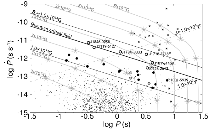
Figure 7: $P-\dot{P}$ diagram for high-B RPPs with the evolutionary track given in Viganò et al. (2013). High-B RPPs are indicated by circles, discriminating between objects showing magnetic activity (open circles) and not (filled circles). Grey circles are objects with weak upper limits. Grey solid line curves indicate simulated evolutionary tracks labelled with the initial dipole magnetic fields ${\it B_{\rm p}^{0}}=3\times 10^{12},10^{13},3^{13},10^{14},3\times 10^{14},10^{15}$G. Star symbols are actual ages $t=10^{3},10^{4},10^{5},5\times 10^{5}$yr. Other symbols are the same as in Figure 1.

In view of theory, we draw the evolutionary tracks of different initial magnetic fields given in Viganò et al. (2013), indicated by the grey lines in the $P-\dot{P}$ diagram in Figure 7. To see properties of high-B PSRs, open circles indicate high-B RPPs with magnetar-like properties such as outbursts, high X-ray efficiency, or high temperature, while black circles indicate high-B RPPs that do not show high efficiency. Other symbols are the same as in Figure 1. According to Viganò et al. (2013), RPPs having high initial magnetic fields larger than ${B_{\rm d}}\gtrsim 1\times 10^{14}$ G will be much more luminous as compared with standard cooling due to additional heating, while RPPs having initial magnetic fields lower than ${B_{\rm d}}\lesssim 1\times 10^{14}$ G will have little effect on X-ray luminosity. Their argument seems to work almost as well. However, PSR J1001$-$5939 in the XINS domain does not follow their argument. Some high-B RPPs with a weaker magnetic field than the quantum magnetic field may evolve with no significant decay of ${B_{\rm d}}$ along straight lines with constant magnetic fields, rather than their evolutional tracks. Future observations of very high-B RPPs such as PSR J1847$-$0130 and PSR J1814$-$1744 are of great importance toward understanding the role of the dipole magnetic field.

In the discussions so far, we have argued that magnetar-like properties appear only when ${\it B_{\rm d}}\gtrsim 10^{13.5}$ G as far as high-B RPPs and detected ordinary PSRs are concerned. However, the number of samples remains small, so this argument would not be conclusive. We should thus perform further observations in the future. It is interesting that magnetars showing persistent emissions are found in the range ${\it B_{\rm d}}\gtrsim 10^{13.5}$ G, while the dipole field strengths of the XINSs extend below $10^{13.5}$ G.

4.2 Probability of high-efficiency RPPs

Let us calculate the probability at which high-efficiency RPPs appear among high-B RPPs. There are 7 high-B RPPs within 2 kpc from the earth in the ATNF pulsar catalogue. Thus, the surface density is 1.75 high-B PSRs kpc^-2, provided that the radio survey is complete within 2 kpc. Three high-efficiency high-B PSRs are located at $\sim 4$ kpc. Using the surface density, the expected number of high-B PSRs within 4 kpc is calculated to be 28. Then the probability of high efficiency appearing in the high-B PSRs is estimated to be 3/28, or approximately 11%. There are five objects having no effective upper limits within 4 kpc. If these objects have high efficiency, the probability will be a higher value: adding these five objects, we would have a maximum probability of 8/28, or approximately 29%.

5 Conclusion

In this work, we performed a systematic analysis of Swift/XRT data for 21 high-B PSRs that had no previously given X-ray flux. As a result, we newly presented $3\sigma$ upper limits for those 21 objects. We found no sources with luminosity comparable to PSR J1819$-$1458, which is a typical high-efficiency X-ray RPP.

The present data suggest that magnetar-like properties appear only when ${\it B_{\rm d}}\gtrsim 10^{13.5}$ G for the high-B RPPs and ordinary PSRs. This observation is in agreement with theoretical predictions for magnetic field evolution, namely that an evolutionary track with an initial toroidal field of $\sim 10^{14}$ G separates observational features (discussed in subsection 4.1; Viganò et al. 2013). It is, however, notable that a few high-B pulsars in the XINS domain might evolve without significant field decay, because of a different evolutionary history for internal magnetic fields.

An increased upper limit allowed us to estimate the probability of high X-ray efficiency to be 11$-$29% in the high-B PSR population.

Appendix A Previous observation data for PSRs and high-B PSRs

Table LABEL:PlotData provides the data used to draw Figure 2, Figure 4, Figure 5 and Figure 6 according to our literature search.

Table 5: Plot data in the $0.3-10$ keV band

PSR name	${\it B_{\rm d}}$	${\it P}$	${\it P_{\rm dot}}$	Distance	log ${\it L_{\rm rot}}$	log ${\it L_{\rm x}}$	Typea	Reference
	G	s	s/s	kpc	erg/s	erg/s
B0114$+$58	7.80$\times 10^{11}$	1.01$\times 10^{-1}$	5.85$\times 10^{-15}$	1.770	35.34	32.74	B0	Prinz & Becker (2015)
B0355$+$54	8.39$\times 10^{11}$	1.56$\times 10^{-1}$	4.40$\times 10^{-15}$	1.000	34.66	30.81	B0	Klingler et al. (2016)
B0531$+$21	3.80$\times 10^{12}$	3.34$\times 10^{-2}$	4.21$\times 10^{-13}$	2.000	38.65	36.33	B0	Kargaltsev et al. (2008)
B0540$+$23	1.97$\times 10^{12}$	2.46$\times 10^{-1}$	1.54$\times 10^{-14}$	1.560	34.61	30.26	B0	Prinz & Becker (2015)
B0540$-$69	4.99$\times 10^{12}$	5.06$\times 10^{-2}$	4.79$\times 10^{-13}$	49.700	38.16	36.49	B0	Kaaret et al. (2001)
B0628$-$28	3.01$\times 10^{12}$	1.24	7.11$\times 10^{-15}$	0.320	32.16	29.35	B0	Tepedelenlıoǧlu & Ögelman (2005)
B0656$+$14	4.66$\times 10^{12}$	3.85$\times 10^{-1}$	5.50$\times 10^{-14}$	0.290	34.58	31.51	B0	Bîrzan et al. (2016)
B0823$+$26	9.64$\times 10^{11}$	5.31$\times 10^{-1}$	1.71$\times 10^{-15}$	0.320	32.65	28.98	B0	Becker et al. (2004)
B0833$-$45	3.39$\times 10^{12}$	8.93$\times 10^{-2}$	1.25$\times 10^{-13}$	0.280	36.84	32.88	B0	Pavlov et al. (2001)
B0905$-$51	6.90$\times 10^{11}$	2.54$\times 10^{-1}$	1.83$\times 10^{-15}$	0.340	33.65	29.53	B0	Bogdanov et al. (2014)
B0906$-$49	1.29$\times 10^{12}$	1.07$\times 10^{-1}$	1.52$\times 10^{-14}$	1.000	35.69	29.85	B0	Kargaltsev et al. (2012)
B0919$+$06	2.46$\times 10^{12}$	4.31$\times 10^{-1}$	1.37$\times 10^{-14}$	1.100	33.83	30.49	B0	Prinz & Becker (2015)
B0950$+$08	2.44$\times 10^{11}$	2.53$\times 10^{-1}$	2.30$\times 10^{-16}$	0.260	32.75	29.92	B0	Becker et al. (2004)
B1046$-$58	3.49$\times 10^{12}$	1.24$\times 10^{-1}$	9.64$\times 10^{-14}$	2.900	36.30	31.53	B0	Kargaltsev et al. (2008)
B1055$-$52	1.09$\times 10^{12}$	1.97$\times 10^{-1}$	5.83$\times 10^{-15}$	0.090	34.48	30.47	B0	Posselt et al. (2015)
B1221$-$63	1.05$\times 10^{12}$	2.16$\times 10^{-1}$	4.95$\times 10^{-15}$	4.000	34.28	31.18	B0	Prinz & Becker (2015)
B1338$-$62	7.08$\times 10^{12}$	1.93$\times 10^{-1}$	2.53$\times 10^{-13}$	12.590	36.14	31.56	B0	Prinz & Becker (2015)
B1706$-$44	3.13$\times 10^{12}$	1.02$\times 10^{-1}$	9.29$\times 10^{-14}$	2.600	36.53	32.87	B0	Romani et al. (2005)
B1757$-$24	4.05$\times 10^{12}$	1.25$\times 10^{-1}$	1.28$\times 10^{-13}$	3.790	36.41	33.10	B0	Kargaltsev et al. (2008)
B1800$-$21	4.29$\times 10^{12}$	1.34$\times 10^{-1}$	1.34$\times 10^{-13}$	4.400	36.35	32.59	B0	Kargaltsev et al. (2007)
B1822$-$09	6.44$\times 10^{12}$	7.69$\times 10^{-1}$	5.25$\times 10^{-14}$	0.300	33.66	30.18	B0	Hermsen et al. (2017)
B1822$-$14	2.55$\times 10^{12}$	2.79$\times 10^{-1}$	2.27$\times 10^{-14}$	4.470	34.61	32.35	B0	Bogdanov et al. (2014)
B1823$-$13	2.80$\times 10^{12}$	1.01$\times 10^{-1}$	7.53$\times 10^{-14}$	3.610	36.45	31.86	B0	Kargaltsev et al. (2008)
B1853$+$01	7.55$\times 10^{12}$	2.67$\times 10^{-1}$	2.08$\times 10^{-13}$	3.300	35.63	31.68	B0	Kargaltsev et al. (2008)
B1929$+$10	5.19$\times 10^{11}$	2.27$\times 10^{-1}$	1.16$\times 10^{-15}$	0.310	33.60	30.30	B0	Misanovic et al. (2008)
B1951$+$32	4.86$\times 10^{11}$	3.95$\times 10^{-2}$	5.83$\times 10^{-15}$	3.000	36.57	33.53	B0	Li et al. (2005)
B2334$+$61	9.91$\times 10^{12}$	4.95$\times 10^{-1}$	1.93$\times 10^{-13}$	0.700	34.80	30.73	B0	McGowan et al. (2006)
J0205$+$6449	3.61$\times 10^{12}$	6.57$\times 10^{-2}$	1.94$\times 10^{-13}$	3.200	37.43	34.02	B0	Kuiper et al. (2010)
J0538$+$2817	7.35$\times 10^{11}$	1.43$\times 10^{-1}$	3.67$\times 10^{-15}$	1.300	34.69	32.67	B0	Ng et al. (2007)
J0729$-$1448	5.40$\times 10^{12}$	2.52$\times 10^{-1}$	1.13$\times 10^{-13}$	2.690	35.45	31.10	B0	Kargaltsev et al. (2012)
J0855$-$4644	6.93$\times 10^{11}$	6.47$\times 10^{-2}$	7.26$\times 10^{-15}$	5.710	36.02	31.08	B0	Maitra et al. (2017)
J1016$-$5857	2.99$\times 10^{12}$	1.07$\times 10^{-1}$	8.07$\times 10^{-14}$	3.160	36.41	31.90	B0	Kargaltsev et al. (2008)
J1028$-$5819	1.23$\times 10^{12}$	9.14$\times 10^{-2}$	1.61$\times 10^{-14}$	1.420	35.92	31.67	B0	Mignani et al. (2012)
J1112$-$6103	1.45$\times 10^{12}$	6.50$\times 10^{-2}$	3.15$\times 10^{-14}$	4.500	36.66	31.78	B0	Prinz & Becker (2015)
J1301$-$6310	6.19$\times 10^{12}$	6.64$\times 10^{-1}$	5.64$\times 10^{-14}$	1.460	33.88	32.34	B0	Prinz & Becker (2015)
J1357$-$6429	7.83$\times 10^{12}$	1.66$\times 10^{-1}$	3.60$\times 10^{-13}$	3.100	36.49	32.58	B0	Chang et al. (2012)
J1400$-$6325	1.12$\times 10^{12}$	3.12$\times 10^{-2}$	3.89$\times 10^{-14}$	7.000	37.70	34.82	B0	Renaud et al. (2010)
J1420$-$6048	2.41$\times 10^{12}$	6.82$\times 10^{-2}$	8.32$\times 10^{-14}$	5.620	37.02	33.12	B0	Kargaltsev et al. (2008)
J1509$-$5850	9.14$\times 10^{11}$	8.89$\times 10^{-2}$	9.16$\times 10^{-15}$	3.350	35.71	31.64	B0	Klingler et al. (2016)
J1524$-$5625	1.77$\times 10^{12}$	7.82$\times 10^{-2}$	3.90$\times 10^{-14}$	3.380	36.51	31.45	B0	Kargaltsev et al. (2012)
J1531$-$5610	1.09$\times 10^{12}$	8.42$\times 10^{-2}$	1.37$\times 10^{-14}$	2.850	35.96	31.67	B0	Kargaltsev et al. (2012)
J1617$-$5055	3.10$\times 10^{12}$	6.94$\times 10^{-2}$	1.35$\times 10^{-13}$	4.740	37.20	34.19	B0	Kargaltsev et al. (2009)
J1702$-$4128	3.13$\times 10^{12}$	1.82$\times 10^{-1}$	5.24$\times 10^{-14}$	3.970	35.53	31.78	B0	Kargaltsev et al. (2012)
J1718$-$3825	1.01$\times 10^{12}$	7.47$\times 10^{-2}$	1.32$\times 10^{-14}$	3.490	36.10	31.96	B0	Kargaltsev et al. (2012)
J1732$-$3131	2.38$\times 10^{12}$	1.97$\times 10^{-1}$	2.80$\times 10^{-14}$	0.640	35.16	30.45	B0	Ray et al. (2011)
J1740$+$1000	1.85$\times 10^{12}$	1.54$\times 10^{-1}$	2.15$\times 10^{-14}$	1.230	35.37	31.88	B0	Kargaltsev et al. (2012)
J1741$-$2054	2.69$\times 10^{12}$	4.14$\times 10^{-1}$	1.70$\times 10^{-14}$	0.300	33.98	31.15	B0	Marelli et al. (2014)
J1747$-$2809	2.89$\times 10^{12}$	5.22$\times 10^{-2}$	1.56$\times 10^{-13}$	8.150	37.64	33.45	B0	Porquet et al. (2003)
J1747$-$2958	2.49$\times 10^{12}$	9.88$\times 10^{-2}$	6.12$\times 10^{-14}$	2.520	36.40	33.28	B0	Gaensler et al. (2004)
J1809$-$1917	1.47$\times 10^{12}$	8.27$\times 10^{-2}$	2.55$\times 10^{-14}$	3.270	36.25	32.13	B0	Kargaltsev & Pavlov (2007)
J1833$-$1034	3.58$\times 10^{12}$	6.19$\times 10^{-2}$	2.02$\times 10^{-13}$	4.100	37.53	34.20	B0	Matheson & Safi-Harb (2010)
J1907$+$0602	3.08$\times 10^{12}$	1.07$\times 10^{-1}$	8.69$\times 10^{-14}$	2.580	36.45	31.79	B0	Abdo et al. (2010)
J2021$+$3651	3.19$\times 10^{12}$	1.04$\times 10^{-1}$	9.57$\times 10^{-14}$	1.800	36.53	32.35	B0	Hessels et al. (2004)
J2022$+$3842	2.07$\times 10^{12}$	4.86$\times 10^{-2}$	8.61$\times 10^{-14}$	10.000	37.47	34.20	B0	Arumugasamy et al. (2014)
J2043$+$2740	3.54$\times 10^{11}$	9.61$\times 10^{-2}$	1.27$\times 10^{-15}$	1.480	34.75	30.76	B0	Abdo et al. (2013)
J2229$+$6114	2.04$\times 10^{12}$	5.16$\times 10^{-2}$	7.83$\times 10^{-14}$	3.000	37.35	32.98	B0	Kargaltsev et al. (2008)
B1509$-$58	1.54$\times 10^{13}$	1.51$\times 10^{-1}$	1.53$\times 10^{-12}$	4.400	37.24	35.13	HB	Kargaltsev et al. (2008)
B1916$+$14	1.60$\times 10^{13}$	1.18	2.12$\times 10^{-13}$	1.300	33.71	30.98	HB	Zhu et al. (2009)
J0007$+$7303b	1.08$\times 10^{13}$	3.16$\times 10^{-1}$	3.60$\times 10^{-13}$	1.400	35.65	31.19	HB	Caraveo et al. (2010)
J0726$-$2612	3.21$\times 10^{13}$	3.44	2.93$\times 10^{-13}$	2.900	32.45	33.24	HB	Speagle et al. (2011)
J1119$-$6127	4.10$\times 10^{13}$	4.08$\times 10^{-1}$	4.02$\times 10^{-12}$	8.400	36.37	33.34	HB	Ng et al. (2012)
J1119$-$6127	4.10$\times 10^{13}$	4.08$\times 10^{-1}$	4.02$\times 10^{-12}$	8.400	36.37	35.54	HBc	Archibald et al. (2016)
J1124$-$5916	1.02$\times 10^{13}$	1.35$\times 10^{-1}$	7.53$\times 10^{-13}$	5.000	37.08	33.31	HB	Hughes et al. (2001)
J1640$-$4631b	1.44$\times 10^{13}$	2.06$\times 10^{-1}$	9.75$\times 10^{-13}$	12.750	36.64	34.56	HB	Gotthelf et al. (2014)
J1718$-$3718	7.46$\times 10^{13}$	3.38	1.61$\times 10^{-12}$	3.920	33.22	32.45	HB	Zhu et al. (2011)
J1734$-$3333	5.24$\times 10^{13}$	1.17	2.28$\times 10^{-12}$	4.460	34.75	32.02	HB	Olausen et al. (2013)
J1819$-$1458	5.01$\times 10^{13}$	4.26	5.75$\times 10^{-13}$	3.300	32.47	33.31	HB	McLaughlin et al. (2007)
J1846$-$0258b	4.89$\times 10^{13}$	3.27$\times 10^{-1}$	7.11$\times 10^{-12}$	5.800	36.91	34.60	HB	Ng et al. (2008)
J1846$-$0258b	4.89$\times 10^{13}$	3.27$\times 10^{-1}$	7.11$\times 10^{-12}$	5.800	36.91	35.26	HBc	Ng et al. (2008)
J1930$+$1852	1.03$\times 10^{13}$	1.37$\times 10^{-1}$	7.52$\times 10^{-13}$	7.000	37.06	34.68	HB	Lu et al. (2007)
J0501$+$4516	1.85$\times 10^{14}$	5.76	5.82$\times 10^{-12}$	2.200	33.08	34.07	Mag	Camero et al. (2014)
J1050$-$5953	5.02$\times 10^{14}$	6.45	3.81$\times 10^{-11}$	9.000	33.75	34.89	Mag	Tam et al. (2008)
J1622$-$4950	2.75$\times 10^{14}$	4.33	1.70$\times 10^{-11}$	5.570	33.92	32.60	Mag	Anderson et al. (2012)
J1708$-$4008	4.70$\times 10^{14}$	1.10$\times 10^{1}$	1.96$\times 10^{-11}$	3.800	32.76	35.19	Mag	Rea et al. (2007)
J1714$-$3810	4.81$\times 10^{14}$	3.82	5.87$\times 10^{-11}$	13.200	34.62	34.79	Mag	Sato et al. (2010)
J1809$-$1943	1.27$\times 10^{14}$	5.54	2.83$\times 10^{-12}$	3.600	32.82	33.92	Mag	Gotthelf et al. (2004)
J1856$+$0245	2.27$\times 10^{12}$	8.09$\times 10^{-2}$	6.21$\times 10^{-14}$	6.320	36.67	33.19	Mag	Rousseau et al. (2012)
J2301$+$5852	5.81$\times 10^{13}$	6.98	4.71$\times 10^{-13}$	3.300	31.74	34.64	Mag	Zhu et al. (2008)
SGR1627$-$41	2.25$\times 10^{14}$	2.59	1.90$\times 10^{-11}$	11.000	34.63	33.66	Mag	Esposito et al. (2008)
RXJ0420.0$-$5022	9.95$\times 10^{12}$	3.45	2.80$\times 10^{-14}$	0.340	31.43	30.33	XINS	Viganò et al. (2013)
RXJ0720.4$-$3125	2.44$\times 10^{13}$	8.39	6.90$\times 10^{-14}$	0.290	30.66	32.09	XINS	Viganò et al. (2013)
RXJ0806.4$-$4123	2.54$\times 10^{13}$	1.14$\times 10^{1}$	5.50$\times 10^{-14}$	0.250	30.17	31.13	XINS	Viganò et al. (2013)
RXJ1308.6$+$2127	3.41$\times 10^{13}$	1.03$\times 10^{1}$	1.10$\times 10^{-13}$	0.500	30.60	32.21	XINS	Viganò et al. (2013)
RXJ1605.3$+$3249	7.46$\times 10^{13}$	3.39	1.60$\times 10^{-12}$	0.350	33.21	31.92	XINS	Viganò et al. (2013)
RXJ1856.5$-$3754	1.47$\times 10^{13}$	7.06	3.00$\times 10^{-14}$	0.120	30.53	31.15	XINS	Viganò et al. (2013)
RXJ2143.0$+$0654	1.99$\times 10^{13}$	9.43	4.10$\times 10^{-14}$	0.430	30.29	31.92	XINS	Viganò et al. (2013)
aNeutron Star population and group. B0, HB, XINS, Mag listed in the type column are PSRs with inferred dipole magnetic field
${\it B_{\rm d}}<10^{13}$G and ${\it F_{\rm rot}}={\it L_{\rm rot}}/4\pi D^{2}>1\times 10^{-11}$, high-B RPPs with inferred dipole magnetic field ${\it B_{\rm d}}\lesssim 10^{13}$G and magnetar population.
bRadio quiet high-B RPPs.
cHigh-B RPPs at Burst.

Table 5: (continued)

References

- Abdo et al. (2010) Abdo, A. A., Ackermann, M., Ajello, M., et al. 2010, ApJ, 711, 64
- Abdo et al. (2013) Abdo, A. A., Ajello, M., Allafort, A., et al. 2013, ApJS, 208, 17
- Anderson et al. (2012) Anderson, G. E., Gaensler, B. M., Slane, P. O., et al. 2012, ApJ, 751, 53
- Archibald et al. (2016) Archibald, R. F., Kaspi, V. M., Tendulkar, S. P., & Scholz, P. 2016, ApJ, 829, L21
- Arumugasamy et al. (2014) Arumugasamy, P., Pavlov, G. G., & Kargaltsev, O. 2014, ApJ, 790, 103
- Becker et al. (2004) Becker, W., Weisskopf, M. C., Tennant, A. F., et al. 2004, ApJ, 615, 908
- Becker et al. (2009) Becker, W. 2009, Astrophysics and Space Science Library, 357, 91
- Becker & Truemper (1997) Becker, W., & Truemper, J. 1997, A&A, 326, 682
- Beskin et al. (2015) Beskin, V. S., Chernov, S. V., Gwinn, C. R., & Tchekhovskoy, A. A. 2015, Space Sci. Rev., 191, 207
- Bogdanov et al. (2014) Bogdanov, S., Ng, C.-Y., & Kaspi, V. M. 2014, ApJ, 792, L36
- Bîrzan et al. (2016) Bîrzan, L., Pavlov, G. G., & Kargaltsev, O. 2016, ApJ, 817, 129
- Burrows et al. (2005) Burrows, D. N., Hill, J. E., Nousek, J. A., et al. 2005, Space Sci. Rev., 120, 165
- Camero et al. (2014) Camero, A., Papitto, A., Rea, N., et al. 2014, MNRAS, 438, 3291
- Caraveo et al. (2010) Caraveo, P. A., De Luca, A., Marelli, M., et al. 2010, ApJ, 725, L6
- Chang et al. (2012) Chang, C., Pavlov, G. G., Kargaltsev, O., & Shibanov, Y. A. 2012, ApJ, 744, 8
- Enoto et al. (2017) Enoto, T., Shibata, S., Kitaguchi, T., et al. 2017, ApJS, 231, 8
- Esposito et al. (2008) Esposito, P., Israel, G. L., Zane, S., et al. 2008, MNRAS, 390, L34 gnami, G. F. 2005, ApJ, 623, 1051
- Esposito et al. (2010) Esposito, P., Israel, G. L., Turolla, R., et al. 2010, MNRAS, 405, 1787
- Dexter et al. (2017) Dexter, J., Degenaar, N., Kerr, M., et al. 2017, MNRAS, 468, 1486
- Gaensler et al. (2004) Gaensler, B. M., van der Swaluw, E., Camilo, F., et al. 2004, ApJ, 616, 383
- Gavriil et al. (2008) Gavriil, F. P., Gonzalez, M. E., Gotthelf, E. V., et al. 2008, Science, 319, 1802
- Gehrels et al. (2004) Gehrels, N., Chincarini, G., Giommi, P., et al. 2004, ApJ, 611, 1005
- Gotthelf et al. (2004) Gotthelf, E. V., Halpern, J. P., Buxton, M., & Bailyn, C. 2004, ApJ, 605, 368
- Gotthelf et al. (2014) Gotthelf, E. V., Tomsick, J. A., Halpern, J. P., et al. 2014, ApJ, 788, 155
- Gehrels (1986) Gehrels, N. 1986, ApJ, 303, 336
- He et al. (2013) He, C., Ng, C.-Y., & Kaspi, V. M. 2013, ApJ, 768, 64
- Hermsen et al. (2017) Hermsen, W., Kuiper, L., Hessels, J. W. T., et al. 2017, MNRAS, 466, 1688
- Hessels et al. (2004) Hessels, J. W. T., Roberts, M. S. E., Ransom, S. M., et al. 2004, ApJ, 612, 389
- Hughes et al. (2001) Hughes, J. P., Slane, P. O., Burrows, D. N., et al. 2001, ApJ, 559, L153
- Kaaret et al. (2001) Kaaret, P., Marshall, H. L., Aldcroft, T. L., et al. 2001, ApJ, 546, 1159
- Kargaltsev & Pavlov (2007) Kargaltsev, O., & Pavlov, G. G. 2007, ApJ, 670, 655
- Kargaltsev et al. (2007) Kargaltsev, O., Pavlov, G. G., & Garmire, G. P. 2007, ApJ, 660, 1413
- Kargaltsev et al. (2008) Kargaltsev, O., & Pavlov, G. G. 2008, 40 Years of Pulsars Millisecond Pulsars, Magnetars and More, 983, 171
- Kargaltsev et al. (2009) Kargaltsev, O., Pavlov, G. G., & Wong, J. A. 2009, ApJ, 690, 891
- Kargaltsev et al. (2012) Kargaltsev, O., Durant, M., Pavlov, G. G., & Garmire, G. 2012, ApJS, 201, 37
- Kaspi & Beloborodov (2017) Kaspi, V. M., & Beloborodov, A. 2017, arXiv:1703.00068
- Klingler et al. (2016) Klingler, N., Kargaltsev, O., Rangelov, B., et al. 2016, ApJ, 828, 70
- Klingler et al. (2016) Klingler, N., Rangelov, B., Kargaltsev, O., et al. 2016, ApJ, 833, 253
- Kuiper & Hermsen (2015) Kuiper, L., & Hermsen, W. 2015, MNRAS, 449, 3827
- Kuiper et al. (2010) Kuiper, L., Hermsen, W., Urama, J. O., et al. 2010, A&A, 515, A34
- Li et al. (2005) Li, X. H., Lu, F. J., & Li, T. P. 2005, ApJ, 628, 931
- Lu et al. (2007) Lu, F., Wang, Q. D., Gotthelf, E. V., & Qu, J. 2007, ApJ, 663, 315
- Maitra et al. (2017) Maitra, C., Acero, F., & Venter, C. 2017, A&A, 597, A75
- Manchester et al. (2005) Manchester, R. N., Hobbs, G. B., Teoh, A., & Hobbs, M. 2005, AJ, 129, 1993
- Marelli et al. (2014) Marelli, M., Belfiore, A., Saz Parkinson, P., et al. 2014, ApJ, 790, 51
- Matheson & Safi-Harb (2010) Matheson, H., & Safi-Harb, S. 2010, ApJ, 724, 572
- McGowan et al. (2006) McGowan, K. E., Zane, S., Cropper, M., Vestrand, W. T., & Ho, C. 2006, ApJ, 639, 377
- McLaughlin et al. (2007) McLaughlin, M. A., Rea, N., Gaensler, B. M., et al. 2007, ApJ, 670, 1307
- Mignani et al. (2012) Mignani, R. P., Razzano, M., Esposito, P., et al. 2012, A&A, 543, A130
- Misanovic et al. (2008) Misanovic, Z., Pavlov, G. G., & Garmire, G. P. 2008, ApJ, 685, 1129-1142
- Ng et al. (2007) Ng, C.-Y., Romani, R. W., Brisken, W. F., Chatterjee, S., & Kramer, M. 2007, ApJ, 654, 487
- Ng et al. (2008) Ng, C.-Y., Slane, P. O., Gaensler, B. M., & Hughes, J. P. 2008, ApJ, 686, 508-519
- Ng et al. (2012) Ng, C.-Y., Kaspi, V. M., Ho, W. C. G., et al. 2012, ApJ, 761, 65
- Olausen et al. (2010) Olausen, S. A., Kaspi, V. M., Lyne, A. G., & Kramer, M. 2010, ApJ, 725, 985
- Olausen et al. (2013) Olausen, S. A., Zhu, W. W., Vogel, J. K., et al. 2013, ApJ, 764, 1 764, 1
- Olausen & Kaspi (2014) Olausen, S. A., & Kaspi, V. M. 2014, ApJS, 212, 6
- Pavlov et al. (2001) Pavlov, G. G., Zavlin, V. E., Sanwal, D., Burwitz, V., & Garmire, G. P. 2001, ApJ, 552, L129
- Pivovaroff et al. (2000) Pivovaroff, M. J., Kaspi, V. M., & Gotthelf, E. V. 2000, ApJ, 528, 436
- Pons & Perna (2011) Pons, J. A., & Perna, R. 2011, ApJ, 741, 123
- Porquet et al. (2003) Porquet, D., Decourchelle, A., & Warwick, R. S. 2003, A&A, 401, 197
- Posselt et al. (2015) Posselt, B., Spence, G., & Pavlov, G. G. 2015, ApJ, 811, 96
- Prinz & Becker (2015) Prinz, T., & Becker, W. 2015, arXiv:1511.07713
- Ray et al. (2011) Ray, P. S., Kerr, M., Parent, D., et al. 2011, ApJS, 194, 17
- Rea et al. (2007) Rea, N., Israel, G. L., Oosterbroek, T., et al. 2007, Ap&SS, 308, 505
- Rea et al. (2010) Rea, N., Esposito, P., Turolla, R., et al. 2010, Science, 330, 944
- Rea et al. (2013) Rea, N., Israel, G. L., Pons, J. A., et al. 2013, ApJ, 770, 65
- Renaud et al. (2010) Renaud, M., Marandon, V., Gotthelf, E. V., et al. 2010, ApJ, 716, 663
- Romani et al. (2005) Romani, R. W., Ng, C.-Y., Dodson, R., & Brisken, W. 2005, ApJ, 631, 480
- Rousseau et al. (2012) Rousseau, R., Grondin, M.-H., Van Etten, A., et al. 2012, A&A, 544, A3
- Sato et al. (2010) Sato, T., Bamba, A., Nakamura, R., & Ishida, M. 2010, PASJ, 62, L33
- Seward & Wang (1988) Seward, F. D., & Wang, Z.-R. 1988, ApJ, 332, 199
- Shibata et al. (2016) Shibata, S., Watanabe, E., Yatsu, Y., Enoto, T., & Bamba, A. 2016, ApJ, 833, 59
- Speagle et al. (2011) Speagle, J. S., Kaplan, D. L., & van Kerkwijk, M. H. 2011, ApJ, 743, 183
- Tam et al. (2008) Tam, C. R., Gavriil, F. P., Dib, R., et al. 2008, ApJ, 677, 503-514
- Tepedelenlıoǧlu & Ögelman (2005) Tepedelenlıoǧlu, E., & Ögelman, H. 2005, ApJ, 630, L57
- Turolla et al. (2015) Turolla, R., Zane, S.,& Watts, A. L. 2015, Reports on Progress in Physics, 78, 116901
- Uchiyama et al. (2011) Uchiyama, H., Koyama, K., Matsumoto, H., et al. 2011, PASJ, 63, S865
- Viganò et al. (2013) Viganò, D., Rea, N., Pons, J. A., et al. 2013, MNRAS, 434, 123
- Zhu et al. (2008) Zhu, W., Kaspi, V. M., Dib, R., et al. 2008, ApJ, 686, 520-527
- Zhu et al. (2009) Zhu, W., Kaspi, V. M., Gonzalez, M. E., & Lyne, A. G. 2009, ApJ, 704, 1321
- Zhu et al. (2011) Zhu, W., Kaspi, V. M., McLaughlin, M. A., et al. 2011, American Institute of Physics Conference Series, 1379, 70