Finite-time Analysis of Approximate Policy Iteration for the Linear Quadratic Regulator

Abstract

We study the sample complexity of approximate policy iteration (PI) for the Linear Quadratic Regulator (LQR), building on a recent line of work using LQR as a testbed to understand the limits of reinforcement learning (RL) algorithms on continuous control tasks. Our analysis quantifies the tension between policy improvement and policy evaluation, and suggests that policy evaluation is the dominant factor in terms of sample complexity. Specifically, we show that to obtain a controller that is within $\varepsilon$ of the optimal LQR controller, each step of policy evaluation requires at most $(n+d)^{3}/\varepsilon^{2}$ samples, where $n$ is the dimension of the state vector and $d$ is the dimension of the input vector. On the other hand, only $\log(1/\varepsilon)$ policy improvement steps suffice, resulting in an overall sample complexity of $(n+d)^{3}\varepsilon^{-2}\log(1/\varepsilon)$. We furthermore build on our analysis and construct a simple adaptive procedure based on $\varepsilon$-greedy exploration which relies on approximate PI as a sub-routine and obtains $T^{2/3}$ regret, improving upon a recent result of Abbasi-Yadkori et al. [3].

1 Introduction

With the recent successes of reinforcement learning (RL) on continuous control tasks, there has been a renewed interest in understanding the sample complexity of RL methods. A recent line of work has focused on the Linear Quadratic Regulator (LQR) as a testbed to understand the behavior and trade-offs of various RL algorithms in the continuous state and action space setting. These results can be broadly grouped into two categories: (1) the study of model-based methods which use data to build an estimate of the transition dynamics, and (2) model-free methods which directly estimate the optimal feedback controller from data without building a dynamics model as an intermediate step. Much of the recent progress in LQR has focused on the model-based side, with an analysis of robust control from Dean et al. [14] and certainty equivalence control by Fiechter [19] and Mania et al. [28]. These techniques have also been extended to the online, adaptive setting [1, 15, 13, 4, 31]. On the other hand, for classic model-free RL algorithms such as Q-learning, SARSA, and approximate policy iteration (PI), our understanding is much less complete despite the fact that these algorithms are well understood in the tabular (finite state and action space) setting. Indeed, most of the model-free analysis for LQR [18, 26, 37] has focused exclusively on derivative-free random search methods.

In this paper, we extend our understanding of model-free algorithms for LQR by studying the performance of approximate PI on LQR, which is a classic approximate dynamic programming algorithm. Approximate PI is a model-free algorithm which iteratively uses trajectory data to estimate the state-value function associated to the current policy (via e.g. temporal difference learning), and then uses this estimate to greedily improve the policy. A key issue in analyzing approximate PI is to understand the trade-off between the number of policy improvement iterations, and the amount of data to collect for each policy evaluation phase. Our analysis quantifies this trade-off, showing that if least-squares temporal difference learning (LSTD-Q) [11, 22] is used for policy evaluation, then a trajectory of length $\widetilde{O}((n+d)^{3}/\varepsilon^{2})$ for each inner step of policy evaluation combined with $\mathcal{O}(\log(1/\varepsilon))$ outer steps of policy improvement suffices to learn a controller that has $\varepsilon$-error from the optimal controller. This yields an overall sample complexity of $\mathcal{O}((n+d)^{3}\varepsilon^{-2}\log(1/\varepsilon))$. Prior to our work, the only known guarantee for approximate PI on LQR was the asymptotic consistency result of Bradtke [12] in the setting of no process noise.

We also extend our analysis of approximate PI to the online, adaptive LQR setting popularized by Abbasi-Yadkori and Szepesvári [1]. By using a greedy exploration scheme similar to Dean et al. [15] and Mania et al. [28], we prove a $\widetilde{O}(T^{2/3})$ regret bound for a simple adaptive policy improvement algorithm. While the $T^{2/3}$ rate is sub-optimal compared to the $T^{1/2}$ regret from model-based methods [1, 13, 28], our analysis improves the $\widetilde{O}(T^{2/3+\varepsilon})$ regret (for $T\geq C^{1/\varepsilon}$) from the model-free Follow the Leader (FTL) algorithm of Abbasi-Yadkori et al. [3]. To the best of our knowledge, we give the best regret guarantee known for a model-free algorithm. We leave open the question of whether or not a model-free algorithm can achieve optimal $T^{1/2}$ regret.

2 Main Results

In this paper, we consider the following linear dynamical system:

$$x_{t+1}=Ax_{t}+Bu_{t}+w_{t}\>,\>\>w_{t}\sim\mathcal{N}(0,\sigma_{w}^{2}I)\>,\>\>x_{0}\sim\mathcal{N}(0,\Sigma_{0})\>.$$ (2.1)

We let $n$ denote the dimension of the state $x_{t}$ and $d$ denote the dimension of the input $u_{t}$. For simplicity we assume that $d\leq n$, e.g. the system is under-actuated. We fix two positive definite cost matrices $(S,R)$, and consider the infinite horizon average-cost Linear Quadratic Regulator (LQR):

$$J_{\star}:=\min_{\{u_{t}(\cdot)\}}\lim_{T\to\infty}\mathbb{E}\left[\frac{1}{T}\sum_{t=1}^{T}x_{t}^{\mathsf{T}}Sx_{t}+u_{t}^{\mathsf{T}}Ru_{t}\right]\>\>\text{subject to}\>\>\eqref{eq:dynamics}\>.$$ (2.2)

We assume the dynamics matrices $(A,B)$ are unknown to us, and our method of interaction with (2.1) is to choose an input sequence $\{u_{t}\}$ and observe the resulting states $\{x_{t}\}$.

We study the solution to (2.2) using least-squares policy iteration (LSPI), a well-known approximate dynamic programming method in RL introduced by Lagoudakis and Parr [22]. The study of approximate PI on LQR dates back to the Ph.D. thesis of Bradtke [12], where he showed that for noiseless LQR (when $w_{t}=0$ for all $t$), the approximate PI algorithm is asymptotically consistent. In this paper we expand on this result and quantify non-asymptotic rates for approximate PI on LQR.

Notation.

For a positive scalar $x>0$, we let $x_{+}=\max\{1,x\}$. A square matrix $L$ is called stable if $\rho(L)<1$ where $\rho(\cdot)$ denotes the spectral radius of $L$. For a symmetric matrix $M\in\mathbb{R}^{n\times n}$, we let $\mathsf{dlyap}(L,M)$ denote the unique solution to the discrete Lyapunov equation $P=L^{\mathsf{T}}PL+M$. We also let $\mathrm{svec}(M)\in\mathbb{R}^{n(n+1)/2}$ denote the vectorized version of the upper triangular part of $M$ so that $\lVert M\rVert_{F}^{2}=\langle\mathrm{svec}(M),\mathrm{svec}(M)\rangle$. Finally, $\mathrm{smat}(\cdot)$ denotes the inverse of $\mathrm{svec}(\cdot)$, so that $\mathrm{smat}(\mathrm{svec}(M))=M$.

2.1 Least-Squares Temporal Difference Learning (LSTD-Q)

The first component towards an understanding of approximate PI is to understand least-squares temporal difference learning (LSTD-Q) for $Q$-functions, which is the fundamental building block of LSPI. Given a policy $K_{\mathrm{eval}}$ which stabilizes $(A,B)$, the goal of LSTD-Q is to estimate the parameters of the $Q$-function associated to $K_{\mathrm{eval}}$. Bellman’s equation for infinite-horizon average cost MDPs (c.f. Bertsekas [7]) states that the (relative) $Q$-function associated to a policy $\pi$ satisfies the following fixed-point equation:

$$\lambda+Q(x,u)=c(x,u)+\mathbb{E}_{x^{\prime}\sim p(\cdot|x,u)}[Q(x^{\prime},\pi(x^{\prime}))]\>.$$ (2.3)

Here, $\lambda\in\mathbb{R}$ is a free parameter chosen so that the fixed-point equation holds. LSTD-Q operates under the linear architecture assumption, which states that the $Q$-function can be described as $Q(x,u)=q^{\mathsf{T}}\phi(x,u)$, for a known (possibly non-linear) feature map $\phi(x,u)$. It is well known that LQR satisfies the linear architecture assumption, since we have:

$$Q(x,u) =\mathrm{svec}(Q)^{\mathsf{T}}\mathrm{svec}\left(\begin{bmatrix}x\\ u\end{bmatrix}\begin{bmatrix}x\\ u\end{bmatrix}^{\mathsf{T}}\right)\>,\>\>Q=\begin{bmatrix}S&0\\ 0&R\end{bmatrix}+\begin{bmatrix}A^{\mathsf{T}}\\ B^{\mathsf{T}}\end{bmatrix}V\begin{bmatrix}A&B\end{bmatrix}\>,$$

$$V =\mathsf{dlyap}(A+BK_{\mathrm{eval}},S+K_{\mathrm{eval}}^{\mathsf{T}}RK_{\mathrm{eval}})\>,\>\>\lambda=\left\langle Q,\sigma_{w}^{2}\begin{bmatrix}I\\ K_{\mathrm{eval}}\end{bmatrix}\begin{bmatrix}I\\ K_{\mathrm{eval}}\end{bmatrix}^{\mathsf{T}}\right\rangle\>.$$

Here, we slightly abuse notation and let $Q$ denote the $Q$-function and also the matrix parameterizing the $Q$-function. Now suppose that a trajectory $\{(x_{t},u_{t},x_{t+1})\}_{t=1}^{T}$ is collected. Note that LSTD-Q is an off-policy method (unlike the closely related LSTD estimator for value functions), and therefore the inputs $u_{t}$ can come from any sequence that provides sufficient excitation for learning. In particular, it does not have to come from the policy $K_{\mathrm{eval}}$. In this paper, we will consider inputs of the form:

$$u_{t}=K_{\mathrm{play}}x_{t}+\eta_{t}\>,\>\>\eta_{t}\sim\mathcal{N}(0,\sigma_{\eta}^{2}I)\>,$$ (2.4)

where $K_{\mathrm{play}}$ is a stabilizing controller for $(A,B)$. Once again we emphasize that $K_{\mathrm{play}}\neq K_{\mathrm{eval}}$ in general. The injected noise $\eta_{t}$ is needed in order to provide sufficient excitation for learning. In order to describe the LSTD-Q estimator, we define the following quantities which play a key role throughout the paper:

$$\phi_{t} :=\phi(x_{t},u_{t})\>,\>\>\psi_{t}:=\phi(x_{t},K_{\mathrm{eval}}x_{t})\>,$$

$$f :=\mathrm{svec}\left(\sigma_{w}^{2}\begin{bmatrix}I\\ K_{\mathrm{eval}}\end{bmatrix}\begin{bmatrix}I\\ K_{\mathrm{eval}}\end{bmatrix}^{\mathsf{T}}\right)\>,\>\>c_{t}:=x_{t}^{\mathsf{T}}Sx_{t}+u_{t}^{\mathsf{T}}Ru_{t}\>.$$

The LSTD-Q estimator estimates $q$ via:

$$\widehat{q}:=\left(\sum_{t=1}^{T}\phi_{t}(\phi_{t}-\psi_{t+1}+f)^{\mathsf{T}}\right)^{{\dagger}}\sum_{t=1}^{T}\phi_{t}c_{t}\>.$$ (2.5)

Here, $(\cdot)^{{\dagger}}$ denotes the Moore-Penrose pseudo-inverse. Our first result establishes a non-asymptotic bound on the quality of the estimator $\widehat{q}$, measured in terms of $\lVert\widehat{q}-q\rVert$. Before we state our result, we introduce a key definition that we will use extensively.

Definition 1.

Let $L$ be a square matrix. Let $\tau\geq 1$ and $\rho\in(0,1)$. We say that $L$ is $(\tau,\rho)$-stable if

$$\lVert L^{k}\rVert\leq\tau\rho^{k}\>,\>\>k=0,1,2,...\>.$$

While stability of a matrix is an asymptotic notion, Definition 1 quantifies the degree of stability by characterizing the transient response of the powers of a matrix by the parameter $\tau$. It is closely related to the notion of strong stability from Cohen et al. [13].

With Definition 1 in place, we state our first result for LSTD-Q.

Theorem 2.1.

Fix a $\delta\in(0,1)$. Let policies $K_{\mathrm{play}}$ and $K_{\mathrm{eval}}$ stabilize $(A,B)$, and assume that both $A+BK_{\mathrm{play}}$ and $A+BK_{\mathrm{eval}}$ are $(\tau,\rho)$-stable. Let the initial state $x_{0}\sim\mathcal{N}(0,\Sigma_{0})$ and consider the inputs $u_{t}=K_{\mathrm{play}}x_{t}+\eta_{t}$ with $\eta_{t}\sim\mathcal{N}(0,\sigma_{\eta}^{2}I)$. For simplicity, assume that $\sigma_{\eta}\leq\sigma_{w}$. Let $P_{\infty}$ denote the steady-state covariance of the trajectory $\{x_{t}\}$:

$$P_{\infty}=\mathsf{dlyap}((A+BK_{\mathrm{play}})^{\mathsf{T}},\sigma_{w}^{2}I+\sigma_{\eta}^{2}BB^{\mathsf{T}})\>.$$ (2.6)

Define the proxy variance $\overline{\sigma}^{2}$ by:

$$\overline{\sigma}^{2}:=\tau^{2}\rho^{4}\lVert\Sigma_{0}\rVert+\lVert P_{\infty}\rVert+\sigma_{\eta}^{2}\lVert B\rVert^{2}\>.$$ (2.7)

Suppose that $T$ satisfies:

$$T\geq\widetilde{O}(1)\max\bigg{\{}(n+d)^{2},\frac{\tau^{4}}{\rho^{4}(1-\rho^{2})^{2}}\frac{(n+d)^{4}}{\sigma_{\eta}^{4}}\sigma_{w}^{2}\overline{\sigma}^{2}\lVert K_{\mathrm{play}}\rVert_{+}^{4}\lVert K_{\mathrm{eval}}\rVert_{+}^{8}(\lVert A\rVert^{4}+\lVert B\rVert^{4})_{+}\bigg{\}}\>.$$ (2.8)

Then we have with probability at least $1-\delta$,

$$\lVert\widehat{q}-q\rVert\leq\widetilde{O}(1)\frac{\tau^{2}}{\rho^{2}(1-\rho^{2})}\frac{(n+d)}{\sigma_{\eta}^{2}\sqrt{T}}\sigma_{w}\overline{\sigma}\lVert K_{\mathrm{play}}\rVert_{+}^{2}\lVert K_{\mathrm{eval}}\rVert_{+}^{4}(\lVert A\rVert^{2}+\lVert B\rVert^{2})_{+}\lVert Q^{K_{\mathrm{eval}}}\rVert_{F}\>.$$ (2.9)

Here the $\widetilde{O}(1)$ hides $\operatorname*{polylog}(n,\tau,\lVert\Sigma_{0}\rVert,\lVert P_{\infty}\rVert,\lVert K_{\mathrm{play}}\rVert,T/\delta,1/\sigma_{\eta})$ factors.

Theorem 2.1 states that:

$$T\leq\widetilde{O}\left((n+d)^{4},\frac{1}{\sigma_{\eta}^{4}}\frac{(n+d)^{3}}{\varepsilon^{2}}\right)$$

timesteps are sufficient to achieve error $\lVert\widehat{q}-q\rVert\leq\varepsilon$ w.h.p. Several remarks are in order. First, while the $(n+d)^{4}$ burn-in is likely sub-optimal, the $(n+d)^{3}/\varepsilon^{2}$ dependence is sharp as shown by the asymptotic results of Tu and Recht [37]. Second, the $1/\sigma_{\eta}^{4}$ dependence on the injected excitation noise will be important when we study the online, adaptive setting in Section 2.3. We leave improving the polynomial dependence of the burn-in period to future work.

The proof of Theorem 2.1 appears in Section A and rests on top of several recent advances. First, we build off the work of Abbasi-Yadkori et al. [3] to derive a new basic inequality for LSTD-Q which serves as a starting point for the analysis. Next, we combine the small-ball techniques of Simchowitz et al. [35] with the self-normalized martingale inequalities of Abbasi-Yadkori et al. [2]. While an analysis of LSTD-Q is presented in Abbasi-Yadkori et al. [3] (which builds on the analysis for LSTD from Tu and Recht [36]), a direct application of their result yields a $1/\sigma_{\eta}^{8}$ dependence; the use of self-normalized inequalities is necessary in order to reduce this dependence to $1/\sigma_{\eta}^{4}$.

2.2 Least-Squares Policy Iteration (LSPI)

With Theorem 2.1 in place, we are ready to present the main results for LSPI. We describe two versions of LSPI in Algorithm 1 and Algorithm 2.

Algorithm 1 $\mathsf{LSPIv1}$ for LQR

1:$K_{0}$: initial stabilizing controller,

2:      $N$: number of policy iterations,

3:      $T$: length of rollout,

4:      $\sigma_{\eta}^{2}$: exploration variance,

5:      $\mu$: lower eigenvalue bound.

6:Collect $\mathcal{D}=\{(x_{k},u_{k},x_{k+1})\}_{k=1}^{T}$ with input $u_{k}=K_{0}x_{k}+\eta_{k}$, $\eta_{k}\sim\mathcal{N}(0,\sigma_{\eta}^{2}I)$.

7:for $t=0,...,N-1$ do

8:     $\widehat{Q}_{t}=\mathsf{Proj}_{\mu}(\mathsf{LSTDQ}(\mathcal{D},K_{t}))$.

9:     $K_{t+1}=G(\widehat{Q}_{t})$. [See (2.10).]

10:end for

11:return $K_{N}$.

Algorithm 2 $\mathsf{LSPIv2}$ for LQR

1:$K_{0}$: initial stabilizing controller,

2:      $N$: number of policy iterations,

3:      $T$: length of rollout,

4:      $\sigma_{\eta}^{2}$: exploration variance,

5:      $\mu$: lower eigenvalue bound.

6:for $t=0,...,N-1$ do

7:      Collect $\mathcal{D}_{t}=\{(x_{k}^{(t)},u_{k}^{(t)},x_{k+1}^{(t)})\}_{k=1}^{T}$, $u_{k}^{(t)}=K_{0}x_{k}^{(t)}+\eta_{k}^{(t)}$,$\eta_{k}^{(t)}\sim\mathcal{N}(0,\sigma_{\eta}^{2}I)$.

8:     $\widehat{Q}_{t}=\mathsf{Proj}_{\mu}(\mathsf{LSTDQ}(\mathcal{D},K_{t}))$.

9:     $K_{t+1}=G(\widehat{Q}_{t})$.

10:end for

11:return $K_{N}$.

In Algorithms 1 and 2, $\mathsf{Proj}_{\mu}(\cdot)=\arg\min_{X=X^{\mathsf{T}}:X\succeq\mu\cdot I}\lVert X-\cdot\rVert_{F}$ is the Euclidean projection onto the set of symmetric matrices lower bounded by $\mu\cdot I$. Furthermore, the map $G(\cdot)$ takes an $(n+d)\times(n+d)$ positive definite matrix and returns a $d\times n$ matrix:

$$G\left(\begin{bmatrix}Q_{11}&Q_{12}\\ Q_{12}^{\mathsf{T}}&Q_{22}\end{bmatrix}\right)=-Q_{22}^{-1}Q_{12}^{\mathsf{T}}\>.$$ (2.10)

Algorithm 1 corresponds to the version presented in Lagoudakis and Parr [22], where all the data $\mathcal{D}$ is collected up front and is re-used in every iteration of LSTD-Q. Algorithm 2 is the one we will analyze in this paper, where new data is collected for every iteration of LSTD-Q. The modification made in Algorithm 2 simplifies the analysis by allowing the controller $K_{t}$ to be independent of the data $\mathcal{D}_{t}$ in LSTD-Q. We remark that this does not require the system to be reset after every iteration of LSTD-Q. We leave analyzing Algorithm 1 to future work.

Before we state our main finite-sample guarantee for Algorithm 2, we review the notion of a (relative) value-function. Similarly to (relative) $Q$-functions, the infinite horizon average-cost Bellman equation states that the (relative) value function $V$ associated to a policy $\pi$ satisfies the fixed-point equation:

$$\lambda+V(x)=c(x,\pi(x))+\mathbb{E}_{x^{\prime}\sim p(\cdot|x,\pi(x))}[V(x^{\prime})]\>.$$ (2.11)

For a stabilizing policy $K$, it is well known that for LQR the value function $V(x)=x^{\mathsf{T}}Vx$ with

$$V=\mathsf{dlyap}(A+BK,S+K^{\mathsf{T}}RK)\>,\>\>\lambda=\langle\sigma_{w}^{2}I,V\rangle\>.$$

Once again as we did for $Q$-functions, we slightly abuse notation and let $V$ denote the value function and the matrix that parameterizes the value function. Our main result for Algorithm 2 appears in the following theorem. For simplicity, we will assume that $\lVert S\rVert\geq 1$ and $\lVert R\rVert\geq 1$.

Theorem 2.2.

Fix a $\delta\in(0,1)$. Let the initial policy $K_{0}$ input to Algorithm 2 stabilize $(A,B)$. Suppose the initial state $x_{0}\sim\mathcal{N}(0,\Sigma_{0})$ and that the excitation noise satisfies $\sigma_{\eta}\leq\sigma_{w}$. Recall that the steady-state covariance of the trajectory $\{x_{t}\}$ is

$$P_{\infty}=\mathsf{dlyap}((A+BK_{0})^{\mathsf{T}},\sigma_{w}^{2}I+\sigma_{\eta}^{2}BB^{\mathsf{T}})\>.$$

Let $V_{0}$ denote the value function associated to the initial policy $K_{0}$, and $V_{\star}$ denote the value function associated to the optimal policy $K_{\star}$ for the LQR problem (2.2). Define the variables $\mu,L$ as:

$$\mu :=\min\{\lambda_{\min}(S),\lambda_{\min}(R)\}\>,$$

$$L :=\max\{\lVert S\rVert,\lVert R\rVert\}+2(\lVert A\rVert^{2}+\lVert B\rVert^{2}+1)\lVert V_{0}\rVert_{+}\>.$$

Fix an $\varepsilon>0$ that satisfies:

$$\varepsilon\leq 5\left(\frac{L}{\mu}\right)^{2}\min\left\{1,\frac{2\log(\lVert V_{0}\rVert/\lambda_{\min}(V_{\star}))}{e},\frac{\lVert V_{\star}\rVert^{2}}{8\mu^{2}\log(\lVert V_{0}\rVert/\lambda_{\min}(V_{\star}))}\right\}\>.$$ (2.12)

Suppose we run Algorithm 2 for $N:=N_{0}+1$ policy improvement iterations where

$$N_{0}:=\left\lceil(1+L/\mu)\log\left(\frac{2\log(\lVert V_{0}\rVert/\lambda_{\min}(V_{\star}))}{\varepsilon}\right)\right\rceil\>,$$ (2.13)

and we set the rollout length $T$ to satisfy:

$$T\geq\widetilde{O}(1)\max\bigg{\{} (n+d)^{2},$$

$$\frac{L^{2}}{(1-\mu/L)^{2}}\left(\frac{L}{\mu}\right)^{17}\frac{(n+d)^{4}}{\sigma_{\eta}^{4}}\sigma_{w}^{2}(\lVert\Sigma_{0}\rVert+\lVert P_{\infty}\rVert+\sigma_{\eta}^{2}\lVert B\rVert^{2}),$$

$$\frac{1}{\varepsilon^{2}}\frac{L^{4}}{(1-\mu/L)^{2}}\left(\frac{L}{\mu}\right)^{42}\frac{(n+d)^{3}}{\sigma_{\eta}^{4}}\sigma_{w}^{2}(\lVert\Sigma_{0}\rVert+\lVert P_{\infty}\rVert+\sigma_{\eta}^{2}\lVert B\rVert^{2})\bigg{\}}\>.$$ (2.14)

Then with probability $1-\delta$, we have that each policy $K_{t}$ for $t=1,...,N$ stabilizes $(A,B)$ and furthermore:

$$\lVert K_{N}-K_{\star}\rVert\leq\varepsilon\>.$$

Here the $\widetilde{O}(1)$ hides $\operatorname*{polylog}(n,\tau,\lVert\Sigma_{0}\rVert,\lVert P_{\infty}\rVert,L/\mu,T/\delta,N_{0},1/\sigma_{\eta})$ factors.

Theorem 2.2 states roughly that $T\cdot N\leq\widetilde{O}(\frac{(n+d)^{3}}{\varepsilon^{2}}\log(1/\varepsilon))$ samples are sufficient for LSPI to recover a controller $K$ that is within $\varepsilon$ of the optimal $K_{\star}$. That is, only $\log(1/\varepsilon)$ iterations of policy improvement are necessary, and furthermore more iterations of policy improvement do not necessary help due to the inherent statistical noise of estimating the $Q$-function for every policy $K_{t}$. We note that the polynomial factor in $L/\mu$ is by no means optimal and was deliberately made quite conservative in order to simplify the presentation of the bound. A sharper bound can be recovered from our analysis techniques at the expense of a less concise expression.

It is worth taking a moment to compare Theorem 2.2 to classical results in the RL literature regarding approximate policy iteration. For example, a well known result (c.f. Theorem 7.1 of Lagoudakis and Parr [22]) states that if LSTD-Q is able to return $Q$-function estimates with error $L_{\infty}$ bounded by $\varepsilon$ at every iteration, then letting $\widehat{Q}_{t}$ denote the approximate $Q$-function at the $t$-th iteration of LSPI:

$$\limsup_{t\to\infty}\>\lVert\widehat{Q}_{t}-Q_{\star}\rVert_{\infty}\leq\frac{2\gamma\varepsilon}{(1-\gamma)^{2}}\>.$$

Here, $\gamma$ is the discount factor of the MDP. Theorem 2.2 is qualitatively similar to this result in that we show roughly that $\varepsilon$ error in the $Q$-function estimate translates to $\varepsilon$ error in the estimated policy. However, there are several fundamental differences. First, our analysis does not rely on discounting to show contraction of the Bellman operator. Instead, we use the $(\tau,\rho)$-stability of closed loop system to achieve this effect. Second, our analysis does not rely on $L_{\infty}$ bounds on the estimated $Q$-function, which are generally not possible to achieve with LQR since the $Q$-function is a quadratic function and the states and inputs are not uniformly bounded. And finally, our analysis is non-asymptotic.

The proof of Theorem 2.2 is given in Section B, and combines the estimation guarantee of Theorem 2.1 with a new analysis of policy iteration for LQR, which we believe is of independent interest. Our new policy iteration analysis combines the work of Bertsekas [8] on policy iteration in infinite horizon average cost MDPs with the contraction theory of Lee and Lim [24] for non-linear matrix equations.

2.3 LSPI for Adaptive LQR

We now turn our attention to the online, adaptive LQR problem as studied in Abbasi-Yadkori and Szepesvári [1]. In the adaptive LQR problem, the quantity of interest is the regret, defined as:

$$\mathsf{Regret}(T):=\sum_{t=1}^{T}x_{t}^{\mathsf{T}}Sx_{t}+u_{t}^{\mathsf{T}}Ru_{t}-T\cdot J_{\star}\>.$$ (2.15)

Here, the algorithm is penalized for the cost incurred from learning the optimal policy $K_{\star}$, and must balance exploration (to better learn the optimal policy) versus exploitation (to reduce cost). As mentioned previously, there are several known algorithms which achieve $\widetilde{O}(\sqrt{T})$ regret [1, 4, 31, 13, 28]. However, these algorithms operate in a model-based manner, using the collected data to build a confidence interval around the true dynamics $(A,B)$. On the other hand, the performance of adaptive algorithms which are model-free is less well understood. We use the results of the previous section to give an adaptive model-free algorithm for LQR which achieves $\widetilde{O}(T^{2/3})$ regret, which improves upon the $\widetilde{O}(T^{2/3+\varepsilon})$ regret (for $T\geq C^{1/\varepsilon}$) achieved by the adaptive model-free algorithm of Abbasi-Yadkori et al. [3]. Our adaptive algorithm based on LSPI is shown in Algorithm 3.

Algorithm 3 Online Adaptive Model-free LQR Algorithm

1:Initial stabilizing controller $K^{(0)}$, number of epochs $E$, epoch multiplier $T_{\mathrm{mult}}$, lower eigenvalue bound $\mu$.

2:for $i=0,...,E-1$ do

3:     Set $T_{i}=T_{\mathrm{mult}}2^{i}$.

4:     Set $\sigma_{\eta,i}^{2}=\sigma_{w}^{2}\left(\frac{1}{2^{i}}\right)^{1/3}$.

5:     Set $K^{(i+1)}=\mathsf{LSPIv2}(K_{0}{=}K^{(i)},N{=}\widetilde{O}((i+1)\Gamma_{\star}/\mu),T{=}T_{i},\sigma_{\eta}^{2}{=}\sigma_{\eta,i}^{2})$.

6:end for

Using an analysis technique similar to that in Dean et al. [15], we prove the following $\widetilde{O}(T^{2/3})$ regret bound for Algorithm 3.

Theorem 2.3.

Fix a $\delta\in(0,1)$. Let the initial feedback $K^{(0)}$ stabilize $(A,B)$ and let $V^{(0)}$ denote its associated value function. Also let $K_{\star}$ denote the optimal LQR controller and let $V_{\star}$ denote the optimal value function. Let $\Gamma_{\star}=1+\max\{\lVert A\rVert,\lVert B\rVert,\lVert V^{(0)}\rVert,\lVert V_{\star}\rVert,\lVert K^{(0)}\rVert,\lVert K_{\star}\rVert,\lVert Q\rVert,\lVert R\rVert\}$. Suppose that $T_{\mathrm{mult}}$ is set to:

$$T_{\mathrm{mult}}\geq\widetilde{O}(1)\mathrm{poly}(\Gamma_{\star},n,d,1/\lambda_{\min}(S))\>.$$

and suppose $\mu$ is set to $\mu=\min\{\lambda_{\min}(S),\lambda_{\min}(R)\}$. With probability at least $1-\delta$, we have that the regret of Algorithm 3 satisfies:

$$\mathsf{Regret}(T)\leq\widetilde{O}(1)\mathrm{poly}(\Gamma_{\star},n,d,1/\lambda_{\min}(S))T^{2/3}\>.$$

The proof of Theorem 2.3 appears in Section C. We note that the regret scaling as $T^{2/3}$ in Theorem 2.3 is due to the $1/\sigma_{\eta}^{4}$ dependence from LSTD-Q (c.f. (2.9)). As mentioned previously, the existing LSTD-Q analysis from Abbasi-Yadkori et al. [3] yields a $1/\sigma_{\eta}^{8}$ dependence in LSTD-Q; using this $1/\sigma_{\eta}^{8}$ dependence in the analysis of Algorithm 3 would translate into $T^{4/5}$ regret.

3 Related Work

For model-based methods, in the offline setting Fiechter [19] provided the first PAC-learning bound for infinite horizon discounted LQR using certainty equivalence (nominal) control. Later, Dean et al. [14] use tools from robust control to analyze a robust synthesis method for infinite horizon average cost LQR, which is applicable in regimes of moderate uncertainty when nominal control fails. Mania et al. [28] show that certainty equivalence control actually provides a fast $\mathcal{O}(\varepsilon^{2})$ rate of sub-optimality where $\varepsilon$ is the size of the parameter error, unlike the $\mathcal{O}(\varepsilon)$ sub-optimality guarantee of [19, 14]. For the online adaptive setting, [1, 20, 4, 28, 13] give $\widetilde{O}(\sqrt{T})$ regret algorithms. A key component of model-based algorithms is being able to quantify a confidence interval for the parameter estimate, for which several recent works [35, 16, 33] provide non-asymptotic results.

Turning to model-free methods, Tu and Recht [36] study the behavior of least-squares temporal difference (LSTD) for learning the discounted value function associated to a stabilizing policy. They evaluate the LSPI algorithm studied in this paper empirically, but do not provide any analysis. In terms of policy optimization, most of the work has focused on derivative-free random search methods [18, 26]. Tu and Recht [37] study a special family of LQR instances and characterize the asymptotic behavior of both model-based certainty equivalent control versus policy gradients (REINFORCE), showing that policy gradients has polynomially worse sample complexity. Most related to our work is Abbasi-Yadkori et al. [3], who analyze a model-free algorithm for adaptive LQR based on ideas from online convex optimization. LSTD-Q is a sub-routine of their algorithm, and their analysis incurs a sub-optimal $1/\sigma_{\eta}^{8}$ dependence on the injected exploration noise, which we improve to $1/\sigma_{\eta}^{4}$ using self-normalized martingale inequalities [2]. This improvement allows us to use a simple greedy exploration strategy to obtain $T^{2/3}$ regret. Finally, as mentioned earlier, the Ph.D. thesis of Bradtke [12] presents an asymptotic consistency argument for approximate PI for discounted LQR in the noiseless setting (i.e. $w_{t}=0$ for all $t$).

For the general function approximation setting in RL, Antos et al. [6] and Lazaric et al. [23] analyze variants of LSPI for discounted MDPs where the state space is compact and the action space finite. In Lazaric et al. [23], the policy is greedily updated via an update operator that requires access to the underlying dynamics (and is therefore not implementable). Farahmand et al. [17] extend the results of Lazaric et al. [23] to when the function spaces considered are reproducing kernel Hilbert spaces. Zou et al. [39] give a finite-time analysis of both Q-learning and SARSA, combining the asymptotic analysis of Melo et al. [29] with the finite-time analysis of TD-learning from Bhandari et al. [9]. We note that checking the required assumptions to apply the results of Zou et al. [39] is non-trivial (c.f. Section 3.1, [29]). We are un-aware of any non-asymptotic analysis of LSPI in the average cost setting, which is more difficult as the Bellman operator is no longer a contraction.

Finally, we remark that our LSPI analysis relies on understanding exact policy iteration for LQR, which is closely related to the fixed-point Riccati recurrence (value iteration). An elegant analysis for value iteration is given by Lincoln and Rantzer [25]. Recently, Fazel et al. [18] show that exact policy iteration is a special case of Gauss-Newton and prove linear convergence results. Our analysis, on the other hand, is based on combining the fixed-point theory from Lee and Lim [24] with recent work on policy iteration for average cost problems from Bertsekas [8].

4 Experiments

In this section, we evaluate LSPI in both the non-adaptive offline setting (Section 2.2) as well as the adaptive online setting (Section 2.3). Section G contains more details about both the algorithms we compare to as well as our experimental methodology.

We first look at the performance of LSPI in the non-adaptive, offline setting. Here, we compare LSPI to other popular model-free methods, and the model-based certainty equivalence (nominal) controller (c.f. [28]). For model-free, we look at policy gradients (REINFORCE) (c.f. [38]) and derivative-free optimization (c.f. [27, 26, 30]). We consider the LQR instance $(A,B,S,R)$ with

$$A=\begin{bmatrix}0.95&0.01&0\\ 0.01&0.95&0.01\\ 0&0.01&0.95\end{bmatrix}\>,\>\>B=\begin{bmatrix}1&0.1\\ 0&0.1\\ 0&0.1\end{bmatrix}\>,\>\>S=I_{3}\>,\>\>R=I_{2}\>.$$

We choose an LQR problem where the $A$ matrix is stable, since the model-free methods we consider need to be seeded with an initial stabilizing controller; using a stable $A$ allows us to start at $K_{0}=0_{2\times 3}$. We fix the process noise $\sigma_{w}=1$. The model-based nominal method learns $(A,B)$ using least-squares, exciting the system with Gaussian inputs $u_{t}$ with variance $\sigma_{u}=1$.

For policy gradients and derivative-free optimization, we use the projected stochastic gradient descent (SGD) method with a constant step size $\mu$ as the optimization procedure. For policy iteration, we evaluate both $\mathsf{LSPIv1}$ (Algorithm 1) and $\mathsf{LSPIv2}$ (Algorithm 2). For every iteration of LSTD-Q, we project the resulting $Q$-function parameter matrix onto the set $\{Q:Q\succeq\gamma I\}$ with $\gamma=\min\{\lambda_{\min}(S),\lambda_{\min}(R)\}$. For $\mathsf{LSPIv1}$, we choose $N=15$ by picking the $N\in[5,10,15]$ which results in the best performance after $T=10^{6}$ timesteps. For $\mathsf{LSPIv2}$, we set $(N,T)=(3,333333)$ which yields the lowest cost over the grid $N\in[1,2,3,4,5,6,7]$ and $T$ such that $NT=10^{6}$.

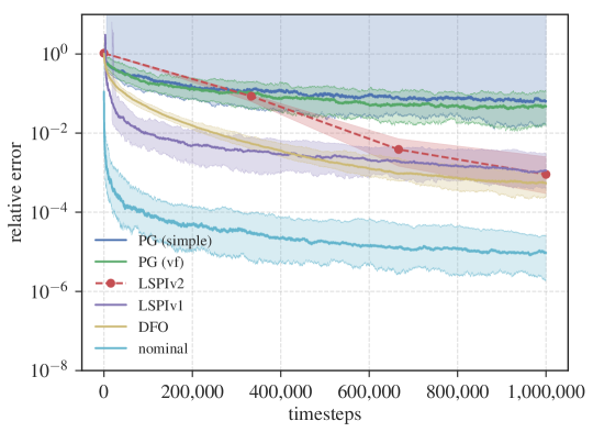
Figure 1: Plot of non-adaptive performance. The shaded regions represent the lower 10th and upper 90th percentile over $100$ trials, and the solid line represents the median performance. Here, PG (simple) is policy gradients with the simple baseline, PG (vf) is policy gradients with the value function baseline, LSPIv2 is Algorithm 2, LSPIv1 is Algorithm 1, and DFO is derivative-free optimization.

Figure 1 contains the results of our non-adaptive evaluation. In Figure 1, we plot the relative error $(J(\widehat{K})-J_{\star})/J_{\star}$ versus the number of timesteps. We see that the model-based certainty equivalence (nominal) method is more sample efficient than the other model-free methods considered. We also see that the value function baseline is able to dramatically reduce the variance of the policy gradient estimator compared to the simple baseline. The DFO method performs the best out of all the model-free methods considered on this example after $10^{6}$ timesteps, although the performance of policy iteration is comparable.

Next, we compare the performance of LSPI in the adaptive setting. We compare LSPI against the model-free linear quadratic control (MFLQ) algorithm of Abbasi-Yadkori et al. [3], the certainty equivalence (nominal) controller (c.f. [15]), and the optimal controller. We set the process noise $\sigma_{w}=1$, and consider the example of Dean et al. [14]:

$$A=\begin{bmatrix}1.01&0.01&0\\ 0.01&1.01&0.01\\ 0&0.01&1.01\end{bmatrix}\>,\>\>B=I_{3}\>,\>\>S=10\cdot I_{3}\>,\>\>R=I_{3}\>.$$

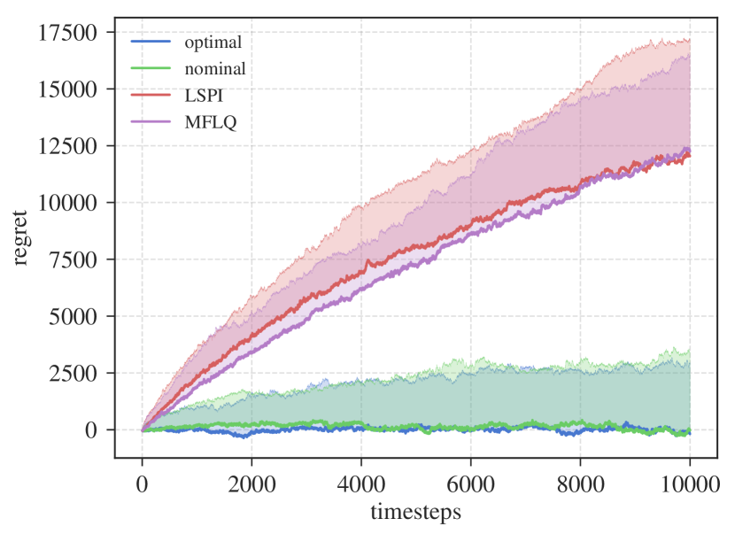
(a) Regret Comparison

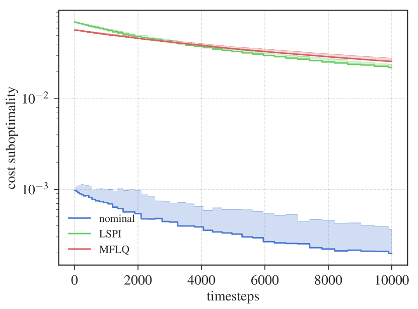
(b) Cost Comparison

Figure 2: Plot of adaptive performance. The shaded regions represent the median to upper 90th percentile over $100$ trials. Here, LSPI is Algorithm 3 using LSPIv1, MFLQ is from Abbasi-Yadkori et al. [3], nominal is the $\varepsilon$-greedy adaptive certainty equivalent controller (c.f. [15]), and optimal has access to the true dynamics. (a) Plot of regret versus time. (b) Plot of the cost sub-optimality versus time.

Figure 2 shows the results of these experiments. In Figure 2(a), we plot the regret (c.f. Equation 2.15) versus the number of timesteps. We see that LSPI and MFLQ both perform similarly with MFLQ slightly outperforming LSPI. We also note that the model-based nominal controller performs significantly better than both LSPI and MFLQ, which is consistent with the experiments of Abbasi-Yadkori et al. [3]. In Figure 2(b), we plot the relative cost $(J(\widehat{K})-J_{\star})/J_{\star}$ versus the number of timesteps. This quantity represents the sub-optimality incurred if further exploration ceases and the current controller is played indefinitely. Here, we see again that LSPI and MFLQ are both comparable, but both are outperformed by nominal control.

5 Conclusion

We studied the sample complexity of approximate PI on LQR, showing that order $(n+d)^{3}\varepsilon^{-2}\log(1/\varepsilon)$ samples are sufficient to estimate a controller that is within $\varepsilon$ of the optimal. We also show how to turn this offline method into an adaptive LQR method with $T^{2/3}$ regret. Several questions remain open with our work. The first is if policy iteration is able to achieve $T^{1/2}$ regret, which is possible with other model-based methods. The second is whether or not model-free methods provide advantages in situations of partial observability for LQ control. Finally, an asymptotic analysis of LSPI, in the spirit of Tu and Recht [37], is of interest in order to clarify which parts of our analysis are sub-optimal due to the techniques we use versus are inherent in the algorithm.

Appendix A Analysis for LSTD-Q

We fix a trajectory $\{(x_{t},u_{t},x_{t+1})\}_{t=1}^{T}$. Recall that we are interested in finding the $Q$ function for a given policy $K_{\mathrm{eval}}$, and we have defined the vectors:

$$\phi_{t} =\phi(x_{t},u_{t})\>,\>\>\psi_{t}=\phi(x_{t},K_{\mathrm{eval}}x_{t})\>,$$

$$f =\mathrm{svec}\left(\sigma_{w}^{2}\begin{bmatrix}I\\ K_{\mathrm{eval}}\end{bmatrix}\begin{bmatrix}I\\ K_{\mathrm{eval}}\end{bmatrix}^{\mathsf{T}}\right)\>,\>\>c_{t}=x_{t}^{\mathsf{T}}Sx_{t}+u_{t}^{\mathsf{T}}Ru_{t}\>.$$

Also recall that the input sequence $u_{t}$ being played is given by $u_{t}=K_{\mathrm{play}}x_{t}+\eta_{t}$, with $\eta_{t}\sim\mathcal{N}(0,\sigma_{\eta}^{2}I)$. Both policies $K_{\mathrm{eval}}$ and $K_{\mathrm{play}}$ are assumed to stabilize $(A,B)$. Because of stability, we have that $P_{t}$ converges to a limit $P_{\infty}=\mathsf{dlyap}((A+BK_{\mathrm{play}})^{\mathsf{T}},\sigma_{w}^{2}I+\sigma_{\eta}^{2}BB^{\mathsf{T}})$, where $P_{t}$ is:

$$P_{t}:=\sum_{k=0}^{t-1}(A+BK_{\mathrm{play}})^{k}(\sigma_{w}^{2}I+\sigma_{\eta}BB^{\mathsf{T}})((A+BK_{\mathrm{play}})^{\mathsf{T}})^{k}\>.$$

The covariance of $x_{t}$ for $t\geq 1$ is:

$$\mathrm{Cov}(x_{t})=\Sigma_{t}:=P_{t}+(A+BK_{\mathrm{play}})^{t}\Sigma_{0}((A+BK_{\mathrm{play}})^{\mathsf{T}})^{t}\>.$$

We define the following data matrices:

$$\Phi=\begin{bmatrix}-\phi_{1}^{\mathsf{T}}-\\ \vdots\\ -\phi_{T}^{\mathsf{T}}-\end{bmatrix}\>,\>\>\Psi_{+}=\begin{bmatrix}-\psi_{2}^{\mathsf{T}}-\\ \vdots\\ -\psi_{T+1}^{\mathsf{T}}-\end{bmatrix}\>,\>\>c=(c_{1},...,c_{T})^{\mathsf{T}}\>,\>\>F=\begin{bmatrix}-f^{\mathsf{T}}-\\ \vdots\\ -f^{\mathsf{T}}-\end{bmatrix}\>.$$

With this notation, the LSTD-Q estimator is:

$$\widehat{q}=\left(\Phi^{\mathsf{T}}(\Phi-\Psi_{+}+F)\right)^{{\dagger}}\Phi^{\mathsf{T}}c\>.$$

Next, let $\Xi$ be the matrix:

$$\Xi=\begin{bmatrix}-\mathbb{E}[\phi(x_{2},K_{\mathrm{eval}}x_{2})|x_{1},u_{1}]^{\mathsf{T}}-\\ \vdots\\ -\mathbb{E}[\phi(x_{T+1},K_{\mathrm{eval}}x_{T+1})|x_{T},u_{T}]^{\mathsf{T}}-\end{bmatrix}\>.$$

For what follows, we let the notation $\otimes_{s}$ denote the symmetric Kronecker product. See Schäcke [34] for more details. The following lemma gives us a starting point for analysis. It is based on Lemma 4.1 of Abbasi-Yadkori et al. [3]. Recall that $q=\mathrm{svec}(Q)$ and $Q$ is the matrix which parameterizes the $Q$-function for $K_{\mathrm{eval}}$.

Lemma A.1 (Lemma 4.1, [3]).

Let $L:=\begin{bmatrix}I\\ K_{\mathrm{eval}}\end{bmatrix}\begin{bmatrix}A&B\end{bmatrix}$. Suppose that $\Phi$ has full column rank, and that

$$\frac{\lVert(\Phi^{\mathsf{T}}\Phi)^{-1/2}\Phi^{\mathsf{T}}(\Xi-\Psi_{+})\rVert}{\sigma_{\mathrm{min}}(\Phi)\sigma_{\mathrm{min}}(I-L\otimes_{s}L)}\leq 1/2\>.$$

Then we have:

$$\lVert\widehat{q}-q\rVert\leq 2\frac{\lVert(\Phi^{\mathsf{T}}\Phi)^{-1/2}\Phi^{\mathsf{T}}(\Xi-\Psi_{+})q\rVert}{\sigma_{\mathrm{min}}(\Phi)\sigma_{\mathrm{min}}(I-L\otimes_{s}L)}\>.$$ (A.1)

Proof.

By the Bellman equation (2.3), we have the identity:

$$\Phi q=c+(\Xi-F)q$$

By the definition of $\widehat{q}$, we have the identity:

$$\Phi\widehat{q}=P_{\Phi}(c+(\Psi_{+}-F)\widehat{q})\>,$$

where $P_{\Phi}=\Phi(\Phi^{\mathsf{T}}\Phi)^{-1}\Phi^{\mathsf{T}}$ is the orthogonal projector onto the columns of $\Phi$. Combining these two identities gives us:

$$P_{\Phi}(\Phi-\Xi+F)(q-\widehat{q})=P_{\Phi}(\Xi-\Psi_{+})\widehat{q}\>.$$

Next, the $i$-th row of $\Phi-\Xi+F$ is:

$$\mathrm{svec}\left(\begin{bmatrix}x_{i}\\ u_{i}\end{bmatrix}\begin{bmatrix}x_{i}\\ u_{i}\end{bmatrix}^{\mathsf{T}}-\mathbb{E}\left[\begin{bmatrix}I\\ K_{\mathrm{eval}}\end{bmatrix}\tilde{x}\tilde{x}^{\mathsf{T}}\begin{bmatrix}I\\ K_{\mathrm{eval}}\end{bmatrix}^{\mathsf{T}}\>\bigg{|}\>x_{i},u_{i}\right]+\sigma_{w}^{2}\begin{bmatrix}I\\ K_{\mathrm{eval}}\end{bmatrix}\begin{bmatrix}I\\ K_{\mathrm{eval}}\end{bmatrix}^{\mathsf{T}}\right)$$

$$\qquad=\mathrm{svec}\left(\begin{bmatrix}x_{i}\\ u_{i}\end{bmatrix}\begin{bmatrix}x_{i}\\ u_{i}\end{bmatrix}^{\mathsf{T}}-L\begin{bmatrix}x_{i}\\ u_{i}\end{bmatrix}\begin{bmatrix}x_{i}\\ u_{i}\end{bmatrix}^{\mathsf{T}}L^{\mathsf{T}}\right)$$

$$\qquad=(I-L\otimes_{s}L)\phi(x_{i},u_{i})\>.$$

Therefore, $\Phi-\Xi+F=\Phi(I-L\otimes_{s}L)^{\mathsf{T}}$. Combining with the above identity:

$$\Phi(I-L\otimes_{s}L)^{\mathsf{T}}(q-\widehat{q})=P_{\Phi}(\Xi-\Psi_{+})\widehat{q}\>.$$

Because $\Phi$ has full column rank, this identity implies that:

$$(I-L\otimes_{s}L)^{\mathsf{T}}(q-\widehat{q})=(\Phi^{\mathsf{T}}\Phi)^{-1}\Phi^{\mathsf{T}}(\Xi-\Psi_{+})\widehat{q}\>.$$

Using the inequalities:

$$\lVert(I-L\otimes_{s}L)^{\mathsf{T}}(q-\widehat{q})\rVert \geq\sigma_{\mathrm{min}}((I-L\otimes_{s}L))\lVert q-\widehat{q}\rVert\>,$$

$$(\Phi^{\mathsf{T}}\Phi)^{-1}\Phi^{\mathsf{T}}(\Xi-\Psi_{+})\widehat{q} \leq\frac{\lVert(\Phi^{\mathsf{T}}\Phi)^{-1/2}\Phi^{\mathsf{T}}(\Xi-\Psi_{+})\widehat{q}\rVert}{\lambda_{\min}((\Phi^{\mathsf{T}}\Phi)^{-1/2})}=\frac{\lVert(\Phi^{\mathsf{T}}\Phi)^{-1/2}\Phi^{\mathsf{T}}(\Xi-\Psi_{+})\widehat{q}\rVert}{\sigma_{\mathrm{min}}(\Phi)}\>,$$

we obtain:

$$\lVert q-\widehat{q}\rVert\leq\frac{\lVert(\Phi^{\mathsf{T}}\Phi)^{-1/2}\Phi^{\mathsf{T}}(\Xi-\Psi_{+})\widehat{q}\rVert}{\sigma_{\mathrm{min}}(\Phi)\sigma_{\mathrm{min}}(I-L\otimes_{s}L)}\>.$$

Next, let $\Delta=q-\widehat{q}$. By triangle inequality:

$$\lVert\Delta\rVert\leq\frac{\lVert(\Phi^{\mathsf{T}}\Phi)^{-1/2}\Phi^{\mathsf{T}}(\Xi-\Psi_{+})\rVert\lVert\Delta\rVert}{\sigma_{\mathrm{min}}(\Phi)\sigma_{\mathrm{min}}(I-L\otimes_{s}L)}+\frac{\lVert(\Phi^{\mathsf{T}}\Phi)^{-1/2}\Phi^{\mathsf{T}}(\Xi-\Psi_{+})q\rVert}{\sigma_{\mathrm{min}}(\Phi)\sigma_{\mathrm{min}}(I-L\otimes_{s}L)}\>.$$

The claim now follows. ∎

In order to apply Lemma A.1, we first bound the minimum singular value $\sigma_{\mathrm{min}}(\Phi)$. We do this using the small-ball argument of Simchowitz et al. [35].

Definition 2 (Definition 2.1, [35]).

Let $\{Z_{t}\}$ be a real-valued stochastic process that is adapted to $\{\mathcal{F}_{t}\}$. The process $\{Z_{t}\}$ satisfies the $(k,\nu,p)$ block martingale small-ball (BMSB) condition if for any $j\geq 0$ we have that:

$$\frac{1}{k}\sum_{i=1}^{k}\mathbb{P}(|Z_{j+i}|\geq\nu|\mathcal{F}_{j})\geq p\>\>\text{a.s.}$$

With the block martingale small-ball definition in place, we now show that the process $\langle\phi_{t},y\rangle$ satisfies this condition for any fixed unit vector $y$.

Proposition A.2.

Given an arbitrary vector $y\in\mathcal{S}^{n+d-1}$, define the process $Z_{t}:=\langle\phi_{t},y\rangle$, the filtration $\mathcal{F}_{t}:=\sigma(\{u_{i},w_{i-1}\}_{i=0}^{t})$, and matrix $C:=\begin{bmatrix}I&0\\ K_{\mathrm{play}}&I\end{bmatrix}\begin{bmatrix}\sigma_{w}I&0\\ 0&\sigma_{\eta}I\end{bmatrix}$. Then $(Z_{t})_{t\geq 1}$ satisfies the $(1,\sigma_{\mathrm{min}}^{2}(C),1/324)$ block martingale small-ball (BMSB) condition from Definition 2. That is, almost surely, we have:

$$\mathbb{P}(|Z_{t+1}|\geq\sigma_{\mathrm{min}}^{2}(C)|\mathcal{F}_{t})\geq 1/324.$$

Proof.

Let $Y:=\mathrm{smat}(y)$ and $\mu_{t}:=Ax_{t}+Bu_{t}$. We have that:

$$\begin{bmatrix}x_{t+1}\\ u_{t+1}\end{bmatrix}=\begin{bmatrix}I\\ K_{\mathrm{play}}\end{bmatrix}\mu_{t}+\begin{bmatrix}I&0\\ K_{\mathrm{play}}&I\end{bmatrix}\begin{bmatrix}w_{t}\\ \eta_{t+1}\end{bmatrix}\>.$$

Therefore:

$$\langle\phi_{t+1},y\rangle =\begin{bmatrix}x_{t+1}\\ u_{t+1}\end{bmatrix}^{\mathsf{T}}Y\begin{bmatrix}x_{t+1}\\ u_{t+1}\end{bmatrix}$$

$$=\left(\begin{bmatrix}I\\ K_{\mathrm{play}}\end{bmatrix}\mu_{t}+\begin{bmatrix}I&0\\ K_{\mathrm{play}}&I\end{bmatrix}\begin{bmatrix}w_{t}\\ \eta_{t+1}\end{bmatrix}\right)^{\mathsf{T}}Y\left(\begin{bmatrix}I\\ K_{\mathrm{play}}\end{bmatrix}\mu_{t}+\begin{bmatrix}I&0\\ K_{\mathrm{play}}&I\end{bmatrix}\begin{bmatrix}w_{t}\\ \eta_{t+1}\end{bmatrix}\right)\>,$$

which is clearly a Gaussian polynomial of degree $2$ given $\mathcal{F}_{t}$. Hence by Gaussian hyper-contractivity results (see e.g. [10]), we have that almost surely:

$$\mathbb{E}[|Z_{t+1}|^{4}|\mathcal{F}_{t}]\leq 81\mathbb{E}[|Z_{t+1}|^{2}|\mathcal{F}_{t}]^{2}.$$

Hence we can invoke the Paley-Zygmund inequality to conclude that for any $\theta\in(0,1)$, almost surely we have:

$$\mathbb{P}(|Z_{t+1}|\geq\sqrt{\theta\mathbb{E}[|Z_{t+1}|^{2}|\mathcal{F}_{t}]}|\mathcal{F}_{t})\geq(1-\theta)^{2}\frac{\mathbb{E}[|Z_{t+1}|^{2}|\mathcal{F}_{t}]^{2}}{\mathbb{E}[|Z_{t+1}|^{4}|\mathcal{F}_{t}]}\geq\frac{(1-\theta)^{2}}{81}.$$

We now state an useful proposition.

Proposition A.3.

Let $\mu,C,Y$ be fixed and $g\sim\mathcal{N}(0,I)$. We have that:

$$\mathbb{E}[((\mu+Cg)^{\mathsf{T}}Y(\mu+Cg))^{2}]\geq 2\lVert C^{\mathsf{T}}YC\rVert_{F}^{2}\>.$$

Proof.

Let $Z:=(\mu+Cg)^{\mathsf{T}}Y(\mu+Cg)$. We know that $\mathbb{E}[Z^{2}]\geq\mathbb{E}[(Z-\mathbb{E}[Z])^{2}]$. A quick computation yields that $\mathbb{E}[Z]=\mu^{\mathsf{T}}Y\mu+\operatorname*{\mathrm{tr}}(C^{\mathsf{T}}YC)$. Hence

$$Z-\mathbb{E}[Z]=g^{\mathsf{T}}C^{\mathsf{T}}YCg-\operatorname*{\mathrm{tr}}(C^{\mathsf{T}}YC)+2\mu^{\mathsf{T}}YCg\>.$$

Therefore,

$$\mathbb{E}[(Z-\mathbb{E}[Z])^{2}]\geq\mathbb{E}[(g^{\mathsf{T}}C^{\mathsf{T}}YCg-\operatorname*{\mathrm{tr}}(C^{\mathsf{T}}YC))^{2}]=2\lVert C^{\mathsf{T}}YC\rVert_{F}^{2}\>.$$

∎

Invoking Proposition A.3 and using basic properties of the Kronecker product, we have that:

$$\mathbb{E}[Z_{t+1}^{2}|\mathcal{F}_{t}]\geq 2\lVert C^{\mathsf{T}}YC\rVert_{F}^{2}=2\lVert(C^{\mathsf{T}}\otimes C^{\mathsf{T}})y\rVert^{2}\geq 2\sigma_{\mathrm{min}}^{2}(C^{\mathsf{T}}\otimes C^{\mathsf{T}})=2\sigma_{\mathrm{min}}^{4}(C)\>.$$

The claim now follows by setting $\theta=1/2$. ∎

With the BMSB bound in place, we can now utilize Proposition 2.5 of Simchowitz et al. [35] to obtain the following lower bound on the minimum singular value $\sigma_{\mathrm{min}}(\Phi)$.

Proposition A.4.

Fix $\delta\in(0,1)$. Suppose that $\sigma_{\eta}\leq\sigma_{w}$, and that $T$ exceeds:

$$T\geq 324^{2}\cdot 8\left((n+d)^{2}\log\left(1+\frac{20736\sqrt{3}}{\sqrt{\delta}}\frac{(1+\lVert K_{\mathrm{play}}\rVert^{2})^{2}(\tau^{2}\rho^{2}n\lVert\Sigma_{0}\rVert+\operatorname*{\mathrm{tr}}(P_{\infty}))}{\sigma_{\eta}^{2}}\right)+\log(2/\delta)\right)\>.$$ (A.2)

Suppose also that $A+BK_{\mathrm{play}}$ is $(\tau,\rho)$-stable. Then we have with probability at least $1-\delta$,

$$\sigma_{\mathrm{min}}(\Phi)\geq\frac{\sigma_{\eta}^{2}}{1296\sqrt{8}}\frac{1}{1+\lVert K_{\mathrm{play}}\rVert^{2}}\sqrt{T}\>.$$

We also have with probability at least $1-\delta$,

$$\lVert\Phi^{\mathsf{T}}\Phi\rVert\leq\frac{12T}{\delta}(1+\lVert K_{\mathrm{play}}\rVert^{2})^{2}(\tau^{2}\rho^{2}n\lVert\Sigma_{0}\rVert+\operatorname*{\mathrm{tr}}(P_{\infty}))^{2}\>.$$

Proof.

We first compute a crude upper bound on $\lVert\Phi\rVert$ using Markov’s inequality:

$$\mathbb{P}(\lVert\Phi\rVert^{2}\geq t^{2})=\frac{\mathbb{E}[\lambda_{\max}(\Phi^{\mathsf{T}}\Phi)]}{t^{2}}\leq\frac{\operatorname*{\mathrm{tr}}(\mathbb{E}[\Phi^{\mathsf{T}}\Phi])}{t^{2}}\>.$$

Now we upper bound $\mathbb{E}[\lVert\phi_{t}\rVert^{2}]$. Letting $z_{t}=(x_{t},u_{t})$, we have that $\mathbb{E}[\lVert\phi_{t}\rVert^{2}]=\mathbb{E}[\lVert z_{t}\rVert^{4}]\leq 3(\mathbb{E}[\lVert z_{t}\rVert^{2}])^{2}$. We now bound $\mathbb{E}[\lVert z_{t}\rVert^{2}]\leq(1+\lVert K_{\mathrm{play}}\rVert^{2})\operatorname*{\mathrm{tr}}(\Sigma_{t})+\sigma_{\eta}^{2}d$, and therefore:

$$\sqrt{\mathbb{E}[\lVert\phi_{t}\rVert^{2}]} \leq\sqrt{3}((1+\lVert K_{\mathrm{play}}\rVert^{2})\operatorname*{\mathrm{tr}}(\Sigma_{t})+\sigma_{\eta}^{2}d)$$

$$\leq\sqrt{3}((1+\lVert K_{\mathrm{play}}\rVert^{2})(\tau^{2}\rho^{2}n\lVert\Sigma_{0}\rVert+\operatorname*{\mathrm{tr}}(P_{\infty}))+\sigma_{\eta}^{2}d)$$

$$\leq 2\sqrt{3}(1+\lVert K_{\mathrm{play}}\rVert^{2})(\tau^{2}\rho^{2}n\lVert\Sigma_{0}\rVert+\operatorname*{\mathrm{tr}}(P_{\infty}))\>.$$

Above, the last inequality holds because $\sigma_{\eta}^{2}d\leq\sigma_{w}^{2}n\leq\operatorname*{\mathrm{tr}}(P_{\infty})$. Therefore, we have from Markov’s inequality:

$$\mathbb{P}\left(\lVert\Phi\rVert\geq\frac{\sqrt{T}}{\sqrt{\delta}}2\sqrt{3}(1+\lVert K_{\mathrm{play}}\rVert^{2})(\tau^{2}\rho^{2}n\lVert\Sigma_{0}\rVert+\operatorname*{\mathrm{tr}}(P_{\infty}))\right)\leq\delta\>.$$

Fix an $\varepsilon>0$, and let $\mathcal{N}(\varepsilon)$ denote an $\varepsilon$-net of the unit sphere $\mathcal{S}^{(n+d)(n+d+1)/2-1}$. Next, by Proposition 2.5 of Simchowitz et al. [35] and a union bound over $\mathcal{N}(\varepsilon)$:

$$\mathbb{P}\left(\min_{v\in\mathcal{N}(\varepsilon)}\lVert\Phi v\rVert\geq\frac{\sigma_{\mathrm{min}}^{2}(C)}{324\sqrt{8}}\sqrt{T}\right)\geq 1-(1+2/\varepsilon)^{(n+d)^{2}}e^{-\frac{T}{324^{2}\cdot 8}}\>.$$

Now set

$$\varepsilon=\frac{\sqrt{\delta}}{5184\sqrt{3}}\frac{\sigma_{\mathrm{min}}^{2}(C)}{(1+\lVert K_{\mathrm{play}}\rVert^{2})(\tau^{2}\rho^{2}n\lVert\Sigma_{0}\rVert+\operatorname*{\mathrm{tr}}(P_{\infty}))}\>,$$

and observe that as long as $T$ exceeds:

$$T\geq 324^{2}\cdot 8\left((n+d)^{2}\log\left(1+\frac{10368\sqrt{3}}{\sqrt{\delta}}\frac{(1+\lVert K_{\mathrm{play}}\rVert^{2})(\tau^{2}\rho^{2}n\lVert\Sigma_{0}\rVert+\operatorname*{\mathrm{tr}}(P_{\infty}))}{\sigma_{\mathrm{min}}^{2}(C)}\right)+\log(2/\delta)\right)\>,$$

we have that $\mathbb{P}\left(\min_{v\in\mathcal{N}(\varepsilon)}\lVert\Phi v\rVert\geq\frac{\sigma_{\mathrm{min}}^{2}(C)}{324\sqrt{8}}\sqrt{T}\right)\geq 1-\delta/2$. To conclude, observe that:

$$\sigma_{\mathrm{min}}(\Phi)=\inf_{\lVert v\rVert=1}\lVert\Phi v\rVert\geq\min_{v\in\mathcal{N}(\varepsilon)}\lVert\Phi v\rVert-\lVert\Phi\rVert\varepsilon\>,$$

and union bound over the two events. To conclude the proof, note that Lemma F.6 in Dean et al. [15] yields that $\sigma_{\mathrm{min}}^{2}(C)\geq\frac{\sigma_{\eta}^{2}}{2}\frac{1}{1+\lVert K_{\mathrm{play}}\rVert^{2}}$ since $\sigma_{\eta}\leq\sigma_{w}$. ∎

We now turn our attention to upper bounding the self-normalized martingale terms:

$$\lVert(\Phi^{\mathsf{T}}\Phi)^{-1}\Phi^{\mathsf{T}}(\Xi-\Psi_{+})\rVert\>\>\text{and}\>\>\lVert(\Phi^{\mathsf{T}}\Phi)^{-1}\Phi^{\mathsf{T}}(\Xi-\Psi_{+})q\rVert\>.$$

Our main tool here will be the self-normalized tail bounds of Abbasi-Yadkori et al. [2].

Lemma A.5 (Corollary 1, [2]).

Let $\{\mathcal{F}_{t}\}$ be a filtration. Let $\{x_{t}\}$ be a $\mathbb{R}^{d_{1}}$ process that is adapted to $\{\mathcal{F}_{t}\}$ and let $\{w_{t}\}$ be a $\mathbb{R}^{d_{2}}$ martingale difference sequence that is adapted to $\{\mathcal{F}_{t}\}$. Let $V$ be a fixed positive definite $d_{1}\times d_{1}$ matrix and define:

$$\bar{V}_{t}=V+\sum_{s=1}^{t}x_{s}x_{s}^{\mathsf{T}}\>,\>\>S_{t}=\sum_{s=1}^{t}x_{s}w_{s+1}^{\mathsf{T}}\>.$$

1. Suppose for any fixed unit $h\in\mathbb{R}^{d_{2}}$ we have that $\langle w_{t},h\rangle$ is conditionally $R$-sub-Gaussian, that is:

   $$\forall\lambda\in\mathbb{R},t\geq 1\>,\>\>\mathbb{E}[e^{\lambda\langle w_{t+1},h\rangle}|\mathcal{F}_{t}]\leq e^{\frac{\lambda^{2}R^{2}}{2}}\>.$$

   We have that with probability at least $1-\delta$, for all $t\geq 1$,

   $$\lVert\bar{V}_{t}^{-1/2}S_{t}\rVert^{2}\leq 8R^{2}\left(d_{2}\log{5}+\log\left(\frac{\det(\bar{V}_{t})^{1/2}\det(V)^{-1/2}}{\delta}\right)\right)\>.$$

2. Now suppose that $\bar{\delta}$ satisfies the condition:

   $$\sum_{s=2}^{T+1}\mathbb{P}(\lVert w_{s}\rVert>R)\leq\bar{\delta}\>.$$

   Then with probability at least $1-\delta-\bar{\delta}$, for all $1\leq t\leq T$,

   $$\lVert\bar{V}_{t}^{-1/2}S_{t}\rVert^{2}\leq 32R^{2}\left(d_{2}\log{5}+\log\left(\frac{\det(\bar{V}_{t})^{1/2}\det(V)^{-1/2}}{\delta}\right)\right)\>.$$

Proof.

Fix a unit $h\in\mathbb{R}^{d_{2}}$. By Corollary 1 of Abbasi-Yadkori et al. [2], we have with probability at least $1-\delta$,

$$\lVert\bar{V}_{t}^{-1/2}S_{t}h\rVert^{2}\leq 2R^{2}\log\left(\frac{\det(\bar{V}_{t})^{1/2}\det(V)^{-1/2}}{\delta}\right)\>,\>\>1\leq t\leq T\>.$$

A standard covering argument yields that:

$$\lVert\bar{V}_{t}^{-1/2}S_{t}\rVert^{2}\leq 4\max_{h\in\mathcal{N}(1/2)}\lVert\bar{V}_{t}^{-1/2}S_{t}h\rVert^{2}\>.$$

Union bounding over $\mathcal{N}(1/2)$, we obtain that:

$$\lVert\bar{V}_{t}^{-1/2}S_{t}\rVert^{2} \leq 8R^{2}\log\left(5^{d_{2}}\frac{\det(\bar{V}_{t})^{1/2}\det(V)^{-1/2}}{\delta}\right)$$

$$=8R^{2}\left(d_{2}\log{5}+\log\left(\frac{\det(\bar{V}_{t})^{1/2}\det(V)^{-1/2}}{\delta}\right)\right)\>.$$

This yields (a).

For (b), we use a simple stopping time argument to handle truncation. Define the stopping time $\tau:=\inf\{t\geq 1:\lVert w_{t}\rVert>R\}$ and the truncated process $\tilde{w}_{t}:=w_{t}\mathbf{1}_{\tau\geq t}$. Because $\tau$ is a stopping time, this truncated process $\{\tilde{w}_{t}\}$ remains a martingale difference sequence. Define $Z_{t}=\sum_{s=1}^{t}x_{s}\tilde{w}_{s+1}^{\mathsf{T}}$. For any $\ell>0$ we observe that:

$$\mathbb{P}(\exists 1\leq t\leq T:\lVert\bar{V}_{t}^{-1/2}S_{t}\rVert>\ell)$$

$$\leq\mathbb{P}(\{\exists 1\leq t\leq T:\lVert\bar{V}_{t}^{-1/2}S_{t}\rVert>\ell\}\cap\{\tau>T+1\})+\mathbb{P}(\tau\leq T+1)$$

$$=\mathbb{P}(\{\exists 1\leq t\leq T:\lVert\bar{V}_{t}^{-1/2}Z_{t}\rVert>\ell\}\cap\{\tau>T+1\})+\mathbb{P}(\tau\leq T+1)$$

$$\leq\mathbb{P}(\exists t\geq 1:\lVert\bar{V}_{t}^{-1/2}Z_{t}\rVert>\ell)+\mathbb{P}(\tau\leq T+1)$$

$$\leq\mathbb{P}(\exists t\geq 1:\lVert\bar{V}_{t}^{-1/2}Z_{t}\rVert>\ell)+\sum_{s=2}^{T+1}\mathbb{P}(\lVert w_{s}\rVert>R)$$

$$\leq\mathbb{P}(\exists t\geq 1:\lVert\bar{V}_{t}^{-1/2}Z_{t}\rVert>\ell)+\bar{\delta}\>.$$

Now set $\ell=32R^{2}\left(d_{2}\log{5}+\log\left(\frac{\det(\bar{V}_{t})^{1/2}\det(V)^{-1/2}}{\delta}\right)\right)$ and using the fact that a $R$ bounded random variable is $2R$-sub-Gaussian, the claim now follows by another application of Corollary 1 from [2]. ∎

With Lemma A.5 in place, we are ready to bound the martingale difference terms.

Proposition A.6.

Suppose the hypothesis of Proposition A.4 hold. With probability at least $1-\delta$,

$$\lVert(\Phi^{\mathsf{T}}\Phi)^{-1/2}\Phi^{\mathsf{T}}(\Xi-\Psi_{+})q\rVert \leq(n+d)\sigma_{w}\sqrt{\tau^{2}\rho^{4}\lVert\Sigma_{0}\rVert+\lVert P_{\infty}\rVert+\sigma_{\eta}^{2}\lVert B\rVert^{2}}(1+\lVert K_{\mathrm{eval}}\rVert^{2})\lVert Q\rVert_{F}$$

$$\qquad\times\operatorname*{polylog}(n,\tau,\lVert\Sigma_{0}\rVert,\lVert P_{\infty}\rVert,\lVert K_{\mathrm{play}}\rVert,T/\delta,1/\sigma_{\eta})\>,$$

$$\lVert(\Phi^{\mathsf{T}}\Phi)^{-1/2}\Phi^{\mathsf{T}}(\Xi-\Psi_{+})\rVert \leq(n+d)^{2}\sigma_{w}\sqrt{\tau^{2}\rho^{4}\lVert\Sigma_{0}\rVert+\lVert P_{\infty}\rVert+\sigma_{\eta}^{2}\lVert B\rVert^{2}}(1+\lVert K_{\mathrm{eval}}\rVert^{2})$$

$$\qquad\times\operatorname*{polylog}(n,\tau,\lVert\Sigma_{0}\rVert,\lVert P_{\infty}\rVert,\lVert K_{\mathrm{play}}\rVert,T/\delta,1/\sigma_{\eta})\>.$$

Proof.

For the proof, constants $c,c_{i}$ will denote universal constants. Define two matrices:

$$V_{1} :=c_{1}\frac{\sigma_{\eta}^{4}}{(1+\lVert K_{\mathrm{play}}\rVert^{2})^{2}}T\cdot I\>,$$

$$V_{2} :=c_{2}\frac{T}{\delta}(1+\lVert K_{\mathrm{play}}\rVert^{2})^{2}(\tau^{2}\rho^{2}n\lVert\Sigma_{0}\rVert+\operatorname*{\mathrm{tr}}(P_{\infty}))^{2}\cdot I\>.$$

By Proposition A.4, with probability at least $1-\delta/2$, we have that:

$$V_{1}\preceq\Phi^{\mathsf{T}}\Phi\preceq V_{2}\>.$$

Call this event $\mathcal{E}_{1}$.

Next, we have:

$$\mathbb{E}[x_{t+1}x_{t+1}^{\mathsf{T}}|x_{t},u_{t}]-x_{t+1}x_{t+1}^{\mathsf{T}}$$

$$=\mathbb{E}[(Ax_{t}+Bu_{t}+w_{t})(Ax_{t}+Bu_{t}+w_{t})^{\mathsf{T}}|x_{t},u_{t}]-(Ax_{t}+Bu_{t}+w_{t})(Ax_{t}+Bu_{t}+w_{t})^{\mathsf{T}}$$

$$=(Ax_{t}+Bu_{t})(Ax_{t}+Bu_{t})^{\mathsf{T}}+\sigma_{w}^{2}I$$

$$\qquad-(Ax_{t}+Bu_{t})(Ax_{t}+Bu_{t})^{\mathsf{T}}-(Ax_{t}+Bu_{t})w_{t}^{\mathsf{T}}-w_{t}(Ax_{t}+Bu_{t})^{\mathsf{T}}-w_{t}w_{t}^{\mathsf{T}}$$

$$=\sigma_{w}^{2}I-w_{t}w_{t}^{\mathsf{T}}-(Ax_{t}+Bu_{t})w_{t}^{\mathsf{T}}-w_{t}(Ax_{t}+Bu_{t})^{\mathsf{T}}\>.$$

Therefore,

$$\mathbb{E}[\psi_{t+1}|x_{t},u_{t}]-\psi_{t+1}$$

$$=\mathrm{svec}\left(\begin{bmatrix}I\\ K_{\mathrm{eval}}\end{bmatrix}(\sigma_{w}^{2}I-w_{t}w_{t}^{\mathsf{T}}-(Ax_{t}+Bu_{t})w_{t}^{\mathsf{T}}-w_{t}(Ax_{t}+Bu_{t})^{\mathsf{T}})\begin{bmatrix}I\\ K_{\mathrm{eval}}\end{bmatrix}^{\mathsf{T}}\right)\>.$$

Taking the inner product of this term with $q$,

$$(\mathbb{E}[\psi_{t+1}|x_{t},u_{t}]-\psi_{t+1})^{\mathsf{T}}q$$

$$=\operatorname*{\mathrm{tr}}\left((\sigma_{w}^{2}I-w_{t}w_{t}^{\mathsf{T}}-(Ax_{t}+Bu_{t})w_{t}^{\mathsf{T}}-w_{t}(Ax_{t}+Bu_{t})^{\mathsf{T}})\begin{bmatrix}I\\ K_{\mathrm{eval}}\end{bmatrix}^{\mathsf{T}}Q\begin{bmatrix}I\\ K_{\mathrm{eval}}\end{bmatrix}\right)$$

$$=\operatorname*{\mathrm{tr}}\left((\sigma_{w}^{2}I-w_{t}w_{t}^{\mathsf{T}})\begin{bmatrix}I\\ K_{\mathrm{eval}}\end{bmatrix}^{\mathsf{T}}Q\begin{bmatrix}I\\ K_{\mathrm{eval}}\end{bmatrix}\right)-2w_{t}^{\mathsf{T}}\begin{bmatrix}I\\ K_{\mathrm{eval}}\end{bmatrix}^{\mathsf{T}}Q\begin{bmatrix}I\\ K_{\mathrm{eval}}\end{bmatrix}(Ax_{t}+Bu_{t})\>.$$

By the Hanson-Wright inequality (see e.g. Rudelson and Vershynin [32]), with probability at least $1-\delta/T$,

$$\left|\operatorname*{\mathrm{tr}}\left((\sigma_{w}^{2}I-w_{t}w_{t}^{\mathsf{T}})\begin{bmatrix}I\\ K_{\mathrm{eval}}\end{bmatrix}^{\mathsf{T}}Q\begin{bmatrix}I\\ K_{\mathrm{eval}}\end{bmatrix}\right)\right|\leq c_{1}\sigma_{w}^{2}(1+\lVert K_{\mathrm{eval}}\rVert^{2})\lVert Q\rVert_{F}\log(T/\delta)\>.$$

Now, let $L_{\mathrm{play}}:=A+BK_{\mathrm{play}}$. By Proposition 4.7 in Tu and Recht [36], with probability at least $1-\delta/T$,

$$\left|w_{t}^{\mathsf{T}}\begin{bmatrix}I\\ K_{\mathrm{eval}}\end{bmatrix}^{\mathsf{T}}Q\begin{bmatrix}I\\ K_{\mathrm{eval}}\end{bmatrix}(Ax_{t}+Bu_{t})\right|$$

$$\leq c_{1}\sigma_{w}(1+\lVert K_{\mathrm{eval}}\rVert^{2})\sqrt{\lVert L_{\mathrm{play}}^{t+1}\Sigma_{0}(L_{\mathrm{play}}^{t+1})^{\mathsf{T}}\rVert+\lVert L_{\mathrm{play}}P_{t}L_{\mathrm{play}}^{\mathsf{T}}\rVert+\sigma_{\eta}^{2}\lVert B\rVert^{2}}\lVert Q\rVert_{F}\log(T/\delta)$$

$$\leq c_{1}\sigma_{w}(1+\lVert K_{\mathrm{eval}}\rVert^{2})\sqrt{\tau^{2}\rho^{2(t+1)}\lVert\Sigma_{0}\rVert+\lVert P_{\infty}\rVert+\sigma_{\eta}^{2}\lVert B\rVert^{2}}\lVert Q\rVert_{F}\log(T/\delta)\>,$$

where the inequality above comes from $P_{t}\preceq P_{\infty}$ and $L_{\mathrm{play}}P_{\infty}L_{\mathrm{play}}^{\mathsf{T}}\preceq P_{\infty}$. Therefore, we have:

$$|(\mathbb{E}[\psi_{t+1}|x_{t},u_{t}]-\psi_{t+1})^{\mathsf{T}}v|$$

$$\leq c_{2}(\sigma_{w}^{2}+\sigma_{w}\sqrt{\tau^{2}\rho^{2(t+1)}\lVert\Sigma_{0}\rVert+\lVert P_{\infty}\rVert+\sigma_{\eta}^{2}\lVert B\rVert^{2}})(1+\lVert K_{\mathrm{eval}}\rVert^{2})\lVert Q\rVert_{F}\log(T/\delta)$$

$$\leq c_{3}\sigma_{w}\sqrt{\tau^{2}\rho^{2(t+1)}\lVert\Sigma_{0}\rVert+\lVert P_{\infty}\rVert+\sigma_{\eta}^{2}\lVert B\rVert^{2}}(1+\lVert K_{\mathrm{eval}}\rVert^{2})\lVert Q\rVert_{F}\log(T/\delta)\>.$$

The last inequality holds because $P_{\infty}\succeq\sigma_{w}^{2}I$ and hence $\sigma_{w}\leq\lVert P_{\infty}\rVert^{1/2}$. Therefore we can set

$$R=c_{3}\sigma_{w}\sqrt{\tau^{2}\rho^{4}\lVert\Sigma_{0}\rVert+\lVert P_{\infty}\rVert+\sigma_{\eta}^{2}\lVert B\rVert^{2}}(1+\lVert K_{\mathrm{eval}}\rVert^{2})\lVert Q\rVert_{F}\log(T/\delta)\>,$$

and invoke Lemma A.5 to conclude that with probability at least $1-\delta/2$,

$$\lVert(V_{1}+\Phi^{\mathsf{T}}\Phi)^{-1/2}\Phi^{\mathsf{T}}(\Xi-\Psi_{+})v\rVert\leq c_{4}(n+d)R+c_{5}R\sqrt{\log(\det((V_{1}+\Phi^{\mathsf{T}}\Phi)V_{1}^{-1})^{1/2}/\delta)}\>.$$

Call this event $\mathcal{E}_{2}$.

For the remainder of the proof we work on $\mathcal{E}_{1}\cap\mathcal{E}_{2}$, which has probability at least $1-\delta$. Since $\Phi^{\mathsf{T}}\Phi\succeq V_{1}$, we have that $(\Phi^{\mathsf{T}}\Phi)^{-1}\leq 2(V_{1}+\Phi^{\mathsf{T}}\Phi)^{-1}$. Therefore, by another application of Lemma A.5:

$$\lVert(\Phi^{\mathsf{T}}\Phi)^{-1/2}\Phi^{\mathsf{T}}(\Xi-\Psi_{+})\rVert$$

$$\leq\sqrt{2}\lVert(V_{1}+\Phi^{\mathsf{T}}\Phi)^{-1/2}\Phi^{\mathsf{T}}(\Xi-\Psi_{+})\rVert$$

$$\leq c_{6}(n+d)R+c_{7}R\sqrt{\log(\det((V_{1}+\Phi^{\mathsf{T}}\Phi)V_{1}^{-1})^{1/2}/\delta)}$$

$$\leq c_{6}(n+d)R+c_{7}R\sqrt{\log(\det((V_{1}+V_{2})V_{1}^{-1})^{1/2}/\delta)}$$

$$\leq c_{6}(n+d)R+c_{8}R(n+d)\sqrt{\log\left(\frac{(1+\lVert K_{\mathrm{play}}\rVert^{2})^{4}}{\delta}\frac{(\tau^{2}\rho^{2}n\lVert\Sigma_{0}\rVert+\operatorname*{\mathrm{tr}}(P_{\infty}))^{2}}{\sigma_{\eta}^{4}}\right)}$$

$$\leq c(n+d)R\operatorname*{polylog}(n,\tau,\lVert\Sigma_{0}\rVert,\lVert P_{\infty}\rVert,\lVert K_{\mathrm{play}}\rVert,1/\delta,1/\sigma_{\eta})\>.$$

Next, we bound:

$$\lVert\mathbb{E}[\psi_{t+1}|x_{t},u_{t}]-\psi_{t+1}\rVert$$

$$\leq\left\lVert\begin{bmatrix}I\\ K_{\mathrm{eval}}\end{bmatrix}(\sigma_{w}^{2}I-w_{t}w_{t}^{\mathsf{T}})\begin{bmatrix}I\\ K_{\mathrm{eval}}\end{bmatrix}^{\mathsf{T}}\right\rVert_{F}+\left\lVert\begin{bmatrix}I\\ K_{\mathrm{eval}}\end{bmatrix}w_{t}(Ax_{t}+Bu_{t})^{\mathsf{T}}\begin{bmatrix}I\\ K_{\mathrm{eval}}\end{bmatrix}^{\mathsf{T}}\right\rVert_{F}$$

$$\leq(1+\lVert K_{\mathrm{eval}}\rVert^{2})(\lVert\sigma_{w}^{2}I-w_{t}w_{t}^{\mathsf{T}}\rVert_{F}+\lVert w_{t}(Ax_{t}+Bu_{t})^{\mathsf{T}}\rVert_{F})\>.$$

Now, by standard Gaussian concentration results, with probability $1-\delta/T$,

$$\lVert\sigma_{w}^{2}I-w_{t}w_{t}^{\mathsf{T}}\rVert_{F} \leq c\sigma_{w}^{2}(n+\log(T/\delta))\>,$$

and also

$$\lVert w_{t}(Ax_{t}+Bu_{t})^{\mathsf{T}}\rVert_{F}$$

$$\leq c\sigma_{w}(\sqrt{n}+\sqrt{\log(T/\delta)})(\sqrt{\operatorname*{\mathrm{tr}}(L_{\mathrm{play}}^{t+1}\Sigma_{0}(L_{\mathrm{play}}^{t+1})^{\mathsf{T}})+\operatorname*{\mathrm{tr}}(L_{\mathrm{play}}P_{t}L_{\mathrm{play}}^{\mathsf{T}})+\sigma_{\eta}^{2}\lVert B\rVert_{F}^{2}}$$

$$\qquad+\sqrt{\lVert L_{\mathrm{play}}^{t+1}\Sigma_{0}(L_{\mathrm{play}}^{t+1})^{\mathsf{T}}\rVert+\lVert L_{\mathrm{play}}P_{t}L_{\mathrm{play}}^{\mathsf{T}}\rVert+\sigma_{\eta}^{2}\lVert B\rVert^{2}}\sqrt{\log(T/\delta)})$$

$$\leq c\sigma_{w}(n+d)\sqrt{\tau^{2}\rho^{4}\lVert\Sigma_{0}\rVert+\lVert P_{\infty}\rVert+\sigma_{\eta}^{2}\lVert B\rVert}\log(T/\delta)\>.$$

Therefore, with probability $1-\delta/T$,

$$\lVert\mathbb{E}[\psi_{t+1}|x_{t},u_{t}]-\psi_{t+1}\rVert$$

$$\leq c(1+\lVert K_{\mathrm{eval}}\rVert^{2})(n+d)\sigma_{w}\sqrt{\tau^{2}\rho^{4}\lVert\Sigma_{0}\rVert+\lVert P_{\infty}\rVert+\sigma_{\eta}^{2}\lVert B\rVert^{2}}\log(T/\delta)\>.$$

∎

We are now in a position to prove Theorem 2.1. We first observe that we can lower bound $\sigma_{\mathrm{min}}(I-L\otimes_{s}L)$ using the $(\tau,\rho)$-stability of $A+BK_{\mathrm{eval}}$. This is because for $k\geq 1$,

$$\lVert L^{k}\rVert =\left\lVert\begin{bmatrix}I\\ K_{\mathrm{eval}}\end{bmatrix}(A+BK_{\mathrm{eval}})^{k-1}\begin{bmatrix}A&B\end{bmatrix}\right\rVert$$

$$\leq 2\lVert K_{\mathrm{eval}}\rVert_{+}\lVert\begin{bmatrix}A&B\end{bmatrix}\rVert\tau\rho^{k-1}$$

$$\leq\frac{2\lVert K_{\mathrm{eval}}\rVert_{+}\max\{1,\sqrt{\lVert A\rVert^{2}+\lVert B\rVert^{2}}\}}{\rho}\tau\cdot\rho^{k}\>.$$

Hence we see that $L$ is $(\frac{2\lVert K_{\mathrm{eval}}\rVert_{+}\max\{1,\sqrt{\lVert A\rVert^{2}+\lVert B\rVert^{2}}\}}{\rho}\tau,\rho)$-stable. Next, we know that $\sigma_{\mathrm{min}}(I-L\otimes_{s}L)=\frac{1}{\lVert(I-L\otimes_{s}L)^{-1}\rVert}$. Therefore, for any unit norm $v$,

$$\lVert(I-L\otimes_{s}L)^{-1}v\rVert =\lVert(I-L\otimes_{s}L)^{-1}\mathrm{svec}(\mathrm{smat}(v))\rVert=\lVert\mathsf{dlyap}(L^{\mathsf{T}},\mathrm{smat}(v))\rVert_{F}$$

$$\leq\frac{4\lVert K_{\mathrm{eval}}\rVert_{+}^{2}(\lVert A\rVert^{2}+\lVert B\rVert^{2})_{+}\tau^{2}}{\rho^{2}(1-\rho^{2})}\>.$$

Here, the last inequality uses Proposition E.5. Hence we have the bound:

$$\sigma_{\mathrm{min}}(I-L\otimes_{s}L)\geq\frac{\rho^{2}(1-\rho^{2})}{4\lVert K_{\mathrm{eval}}\rVert_{+}^{2}(\lVert A\rVert^{2}+\lVert B\rVert^{2})_{+}\tau^{2}}\>.$$

By Proposition A.4, as long as $T\geq\widetilde{O}(1)(n+d)^{2}$ with probability at least $1-\delta/2$:

$$\sigma_{\mathrm{min}}(\Phi)\geq c\frac{\sigma_{\eta}^{2}}{\lVert K_{\mathrm{play}}\rVert_{+}^{2}}\sqrt{T}\>.$$

By Proposition A.6, with probability at least $1-\delta/2$:

$$\lVert(\Phi^{\mathsf{T}}\Phi)^{-1/2}\Phi^{\mathsf{T}}(\Xi-\Psi_{+})q\rVert \leq(n+d)\sigma_{w}\sqrt{\tau^{2}\rho^{4}\lVert\Sigma_{0}\rVert+\lVert P_{\infty}\rVert+\sigma_{\eta}^{2}\lVert B\rVert^{2}}\lVert K_{\mathrm{eval}}\rVert^{2}_{+}\lVert Q^{K_{\mathrm{eval}}}\rVert_{F}\widetilde{O}(1)\>,$$

$$\lVert(\Phi^{\mathsf{T}}\Phi)^{-1/2}\Phi^{\mathsf{T}}(\Xi-\Psi_{+})\rVert \leq(n+d)^{2}\sigma_{w}\sqrt{\tau^{2}\rho^{4}\lVert\Sigma_{0}\rVert+\lVert P_{\infty}\rVert+\sigma_{\eta}^{2}\lVert B\rVert^{2}}\lVert K_{\mathrm{eval}}\rVert^{2}_{+}\widetilde{O}(1)\>.$$

We first check the condition

$$\frac{\lVert(\Phi^{\mathsf{T}}\Phi)^{-1/2}\Phi^{\mathsf{T}}(\Xi-\Psi_{+})\rVert}{\sigma_{\mathrm{min}}(\Phi)\sigma_{\mathrm{min}}(I-L\otimes_{s}L)}\leq 1/2\>,$$

from Lemma A.1. A sufficient condition is that $T$ satisfies:

$$T \geq\widetilde{O}(1)\frac{\lVert K_{\mathrm{play}}\rVert_{+}^{4}}{\sigma_{\eta}^{4}}\cdot(n+d)^{4}\sigma_{w}^{2}(\tau^{2}\rho^{4}\lVert\Sigma_{0}\rVert+\lVert P_{\infty}\rVert+\sigma_{\eta}^{2}\lVert B\rVert^{2})$$

$$\qquad\times\lVert K_{\mathrm{eval}}\rVert_{+}^{4}\cdot\frac{\lVert K_{\mathrm{eval}}\rVert_{+}^{4}(\lVert A\rVert^{2}+\lVert B\rVert^{2})_{+}^{2}\tau^{4}}{\rho^{4}(1-\rho^{2})^{2}}$$

$$=\widetilde{O}(1)\frac{\tau^{4}}{\rho^{4}(1-\rho^{2})^{2}}\frac{(n+d)^{4}}{\sigma_{\eta}^{4}}\sigma_{w}^{2}(\tau^{2}\rho^{4}\lVert\Sigma_{0}\rVert+\lVert P_{\infty}\rVert+\sigma_{\eta}^{2}\lVert B\rVert^{2})$$

$$\qquad\times\lVert K_{\mathrm{play}}\rVert_{+}^{4}\lVert K_{\mathrm{eval}}\rVert_{+}^{8}(\lVert A\rVert^{4}+\lVert B\rVert^{4})_{+}\>.$$

Once this condition on $T$ is satisfied, then we have that the error $\lVert\widehat{q}-q\rVert$ is bounded by:

$$\widetilde{O}(1)\frac{\lVert K_{\mathrm{play}}\rVert_{+}^{2}}{\sigma_{\eta}^{2}\sqrt{T}}\cdot(n+d)\sigma_{w}\sqrt{\tau^{2}\rho^{4}\lVert\Sigma_{0}\rVert+\lVert P_{\infty}\rVert+\sigma_{\eta}^{2}\lVert B\rVert^{2}}$$

$$\qquad\times\lVert K_{\mathrm{eval}}\rVert^{2}_{+}\lVert Q^{K_{\mathrm{eval}}}\rVert_{F}\cdot\frac{\lVert K_{\mathrm{eval}}\rVert_{+}^{2}(\lVert A\rVert^{2}+\lVert B\rVert^{2})_{+}\tau^{2}}{\rho^{2}(1-\rho^{2})}$$

$$=\widetilde{O}(1)\frac{\tau^{2}}{\rho^{2}(1-\rho^{2})}\frac{(n+d)}{\sigma_{\eta}^{2}\sqrt{T}}\sigma_{w}\sqrt{\tau^{2}\rho^{4}\lVert\Sigma_{0}\rVert+\lVert P_{\infty}\rVert+\sigma_{\eta}^{2}\lVert B\rVert^{2}}$$

$$\qquad\times\lVert K_{\mathrm{play}}\rVert_{+}^{2}\lVert K_{\mathrm{eval}}\rVert_{+}^{4}(\lVert A\rVert^{2}+\lVert B\rVert^{2})_{+}\lVert Q^{K_{\mathrm{eval}}}\rVert_{F}\>.$$

Theorem 2.1 now follows from Lemma A.1.

Appendix B Analysis for LSPI

In this section we study the non-asymptotic behavior of LSPI. Our analysis proceeds in two steps. We first understand the behavior of exact policy iteration on LQR. Then, we study the effects of introducing errors into the policy iteration updates.

B.1 Exact Policy Iteration

Exactly policy iteration works as follows. We start with a stabilizing controller $K_{0}$ for $(A,B)$, and let $V_{0}$ denote its associated value function. We then apply the following recursions for $t=0,1,2,...$:

$$K_{t+1} =-(S+B^{\mathsf{T}}V_{t}B)^{-1}B^{\mathsf{T}}V_{t}A\>,$$ (B.1)

$$V_{t+1} =\mathsf{dlyap}(A+BK_{t+1},S+K_{t+1}^{\mathsf{T}}RK_{t+1})\>.$$ (B.2)

Note that this recurrence is related to, but different from, that of value iteration, which starts from a PSD $V_{0}$ and recurses:

$$V_{t+1}=A^{\mathsf{T}}V_{t}A-A^{\mathsf{T}}V_{t}B(S+B^{\mathsf{T}}V_{t}B)^{-1}B^{\mathsf{T}}V_{t}A+S\>.$$

While the behavior of value iteration for LQR is well understood (see e.g. Lincoln and Rantzer [25] or Kailath et al. [21]), the behavior of policy iteration is less studied. Fazel et al. [18] show that policy iteration is equivalent to the Gauss-Newton method on the objective $J(K)$ with a specific step-size, and give a simple analysis which shows linear convergence to the optimal controller. In this section, we present an analysis of the behavior of exact policy iteration that builds on top of the fixed-point theory from Lee and Lim [24]. A key component of our analysis is the following invariant metric $\delta_{\infty}$ on positive definite matrices:

$$\delta_{\infty}(A,B):=\lVert\log(A^{-1/2}BA^{-1/2})\rVert\>.$$

Various properties of $\delta_{\infty}$ are reviewed in Appendix D.

Our analysis proceeds as follows. First, we note by the matrix inversion lemma:

$$S+A^{\mathsf{T}}(BR^{-1}B^{\mathsf{T}}+V^{-1})^{-1}A=S+A^{\mathsf{T}}VA-A^{\mathsf{T}}VB(R+B^{\mathsf{T}}VB)^{-1}B^{\mathsf{T}}VA=:F(V)\>.$$

Let $V_{\star}$ be the unique positive definite solution to $V=F(V)$. For any positive definite $V$ we have by Lemma D.2:

$$\delta_{\infty}(F(V),V_{\star})\leq\frac{\alpha}{\lambda_{\min}(S)+\alpha}\delta_{\infty}(V,V_{\star})\>,$$ (B.3)

with $\alpha=\max\{\lambda_{\max}(A^{\mathsf{T}}VA),\lambda_{\max}(A^{\mathsf{T}}V_{\star}A)\}$. Indeed, (B.3) gives us another method to analyze value iteration, since it shows that the Riccati operator $F(V)$ is contractive in the $\delta_{\infty}$ metric. Our next result combines this contraction property with the policy iteration analysis of Bertsekas [8].

Proposition B.1 (Policy Iteration for LQR).

Suppose that $S,R$ are positive definite and there exists a unique positive definite solution to the discrete algebraic Riccati equation (DARE). Let $K_{0}$ be a stabilizing policy for $(A,B)$ and let $V_{0}=\mathsf{dlyap}(A+BK_{0},S+K_{0}^{\mathsf{T}}RK_{0})$. Consider the following sequence of updates for $t=0,1,2,...$:

$$K_{t+1} =-(R+B^{\mathsf{T}}V_{t}B)^{-1}B^{\mathsf{T}}V_{t}A\>,$$

$$V_{t+1} =\mathsf{dlyap}(A+BK_{t+1},S+K_{t+1}^{\mathsf{T}}RK_{t+1})\>.$$

The following statements hold:

1. $K_{t}$ stabilizes $(A,B)$ for all $t=0,1,2,...$,

2. $V_{\star}\preceq V_{t+1}\preceq V_{t}$ for all $t=0,1,2,...$,

3. $\delta_{\infty}(V_{t+1},V_{\star})\leq\rho\cdot\delta_{\infty}(V_{t},V_{\star})$ for all $t=0,1,2,...$, with $\rho:=\frac{\lambda_{\max}(A^{\mathsf{T}}V_{0}A)}{\lambda_{\min}(S)+\lambda_{\max}(A^{\mathsf{T}}V_{0}A)}$. Consequently, $\delta_{\infty}(V_{t},V_{\star})\leq\rho^{t}\cdot\delta_{\infty}(V_{0},V_{\star})$ for $t=0,1,2,...$.

Proof.

We first prove (i) and (ii) using the argument of Proposition 1.3 from Bertsekas [8].

Let $c(x,u)=x^{\mathsf{T}}Sx+u^{\mathsf{T}}Ru$, $f(x,u)=Ax+Bu$, and $V^{K}(x_{1})=\sum_{t=1}^{\infty}c(x_{t},u_{t})$ with $x_{t+1}=f(x_{t},u_{t})$ and $u_{t}=Kx_{t}$. Let $V_{t}=V^{K_{t}}$. With these definitions, we have that for all $x$:

$$K_{t+1}x=\arg\min_{u}c(x,u)+V_{t}(f(x,u))\>.$$

Therefore,

$$V_{t}(x) =c(x,K_{t}x)+V_{t}(f(x,K_{t}x))$$

$$\geq c(x,K_{t+1}x)+V_{t}(f(x,K_{t+1}x))$$

$$=c(x,K_{t+1}x)+c(f(x,K_{t+1}x),K_{t}f(x,K_{t+1}x))+V_{t}(f(f(x,K_{t+1}x),K_{t}f(x,K_{t+1}x)))$$

$$\geq c(x,K_{t+1}x)+c(f(x,K_{t+1}x),K_{t+1}f(x,K_{t+1}x))+V_{t}(f(f(x,K_{t+1}x),K_{t+1}f(x,K_{t+1}x)))$$

$$\vdots$$

$$\geq V_{t+1}(x)\>.$$

This proves (i) and (ii).

Now, observe that by partial minimization of a strongly convex quadratic:

$$c(x,K_{t+1}x)+V_{t}(f(x,K_{t+1}x)) =\min_{u}c(x,u)+V_{t}(f(x,u))$$

$$=x^{\mathsf{T}}(S+A^{\mathsf{T}}V_{t}A-A^{\mathsf{T}}V_{t}B(R+B^{\mathsf{T}}V_{t}B)^{-1}B^{\mathsf{T}}V_{t}A)x$$

$$=x^{\mathsf{T}}F(V_{t})x\>.$$

Combined with the above inequalities, this shows that $V_{t+1}\preceq F(V_{t})\preceq V_{t}$. Therefore, by (B.3) and Proposition D.4,

$$\delta_{\infty}(V_{t+1},V_{\star}) \leq\delta_{\infty}(F(V_{t}),V_{\star})$$

$$=\delta_{\infty}(F(V_{t}),F(V_{\star}))$$

$$\leq\frac{\alpha_{t}}{\lambda_{\min}(Q)+\alpha_{t}}\delta_{\infty}(V_{t},V_{\star})\>,$$

where $\alpha_{t}=\max\{\lambda_{\max}(A^{\mathsf{T}}V_{t}A),\lambda_{\max}(A^{\mathsf{T}}V_{\star}A)\}=\lambda_{\max}(A^{\mathsf{T}}V_{t}A)$, since $V_{\star}\preceq V_{t}$. But since $V_{t}\preceq V_{0}$, we can upper bound $\alpha_{t}\leq\lambda_{\max}(A^{\mathsf{T}}V_{0}A)$. This proves (iii). ∎

B.2 Approximate Policy Iteration

We now turn to the analysis of approximate policy iteration. Before analyzing Algorithm 2, we analyze a slightly more general algorithm described in Algorithm 4

Algorithm 4 Approximate Policy Iteration for LQR (offline)

1:Initial stabilizing controller $K_{0}$, $N$ number of policy iterations, $T$ length of rollout for estimation, $\sigma_{\eta}^{2}$ exploration variance.

2:for $t=0,...,N-1$ do

3:     Collect a trajectory $\mathcal{D}_{t}=\{(x_{k}^{(t)},u_{k}^{(t)},x_{k+1}^{(t)})\}_{k=1}^{T}$ using input $u_{k}^{(t)}=K_{0}x_{k}^{(t)}+\eta_{k}^{(t)}$, with $\eta_{k}^{(t)}\sim\mathcal{N}(0,\sigma_{\eta}^{2}I)$.

4:     $\widehat{Q}_{t}=\mathsf{EstimateQ}(\mathcal{D}_{t},K_{t})$.

5:     $K_{t+1}=G(\widehat{Q}_{t})$. [c.f. (2.10)]

6:end for

7:return $K_{N}$.

In Algorithm 4, the procedure $\mathsf{EstimateQ}$ takes as input an off-policy trajectory $\mathcal{D}_{t}$ and a policy $K_{t}$, and returns an estimate $\widehat{Q}_{t}$ of the true $Q$ function $Q_{t}$. We will analyze Algorithm 4 first assuming that the procedure $\mathsf{EstimateQ}$ delivers an estimate with a certain level of accuracy. In order to do this, we define the sequence of variables:

1. $Q_{t}$ is true state-value function for $K_{t}$.

2. $V_{t}$ is true value function for $K_{t}$.

3. $\overline{K}_{t+1}=G(Q_{t})$.

4. $\overline{V}_{t}$ is true value function for $\overline{K}_{t}$.

The following proposition is our main result regarding Algorithm 4.

Proposition B.2.

Consider the sequence of updates defined by Algorithm 4. Suppose we start with a stabilizing $K_{0}$ and let $V_{0}$ denote its value function. Fix an $\varepsilon>0$. Define the following variables:

$$\mu :=\min\{\lambda_{\min}(S),\lambda_{\min}(R)\}\>,$$

$$Q_{\max} :=\max\{\lVert S\rVert,\lVert R\rVert\}+2(\lVert A\rVert^{2}+\lVert B\rVert^{2})\lVert V_{0}\rVert\>,$$

$$\gamma :=\frac{2\lVert A\rVert^{2}\lVert V_{0}\rVert}{\mu+2\lVert A\rVert^{2}\lVert V_{0}\rVert}\>,$$

$$N_{0} :=\lceil\frac{1}{1-\gamma}\log(2\delta_{\infty}(V_{0},V_{\star})/\varepsilon)\rceil\>,$$

$$\tau :=\sqrt{\frac{2\lVert V_{0}\rVert}{\mu}}\>,$$

$$\rho :=\sqrt{1-1/\tau^{2}}\>,$$

$$\overline{\rho} :=\mathsf{Avg}(\rho,1)\>.$$

Let $N_{1}\geq N_{0}$. Suppose the estimates $\widehat{Q}_{t}$ output by $\mathsf{EstimateQ}$ satisfy, for all $0\leq t\leq N_{1}-1$, $\widehat{Q}_{t}\succeq\mu I$ and furthermore,

$$\lVert\widehat{Q}_{t}-Q_{t}\rVert \leq\min\left\{\frac{\lVert V_{0}\rVert}{N_{1}},\varepsilon\mu(1-\gamma)\right\}\left(\frac{\mu}{28}\frac{(1-\overline{\rho}^{2})^{2}}{\tau^{5}}\frac{1}{\lVert B\rVert_{+}\max\{\lVert S\rVert,\lVert R\rVert\}}\frac{\mu^{3}}{Q_{\max}^{3}}\right)\>.$$

Then we have for any $N$ satisfying $N_{0}\leq N\leq N_{1}$ the bound $\delta_{\infty}(V_{N},V_{\star})\leq\varepsilon$. We also have that for all $0\leq t\leq N_{1}$, $A+BK_{t}$ is $(\tau,\overline{\rho})$-stable and $\lVert K_{t}\rVert\leq 2Q_{\max}/\mu$.

Proof.

We first start by observing that if $V,V_{0}$ are value functions satisfying $V\preceq V_{0}$, then their state-value functions also satisfy $Q\preceq Q_{0}$. This is because

$$Q =\begin{bmatrix}S&0\\ 0&R\end{bmatrix}+\begin{bmatrix}A^{\mathsf{T}}\\ B^{\mathsf{T}}\end{bmatrix}V\begin{bmatrix}A&B\end{bmatrix}$$

$$\preceq\begin{bmatrix}S&0\\ 0&R\end{bmatrix}+\begin{bmatrix}A^{\mathsf{T}}\\ B^{\mathsf{T}}\end{bmatrix}V_{0}\begin{bmatrix}A&B\end{bmatrix}=Q_{0}\>.$$

From this we also see that any state-value function satisfies $Q\succeq\begin{bmatrix}S&0\\ 0&R\end{bmatrix}$.

The proof proceeds as follows. We observe that since $\overline{V}_{t+1}\preceq V_{t}$ (Proposition B.1-(ii)):

$$V_{t} =V_{t}-\overline{V}_{t}+\overline{V}_{t}-V_{t-1}+V_{t-1}\preceq V_{t}-\overline{V}_{t}+V_{t-1}\>.$$

Therefore, by triangle inequality we have $\lVert V_{t}\rVert\leq\lVert V_{t}-\overline{V}_{t}\rVert+\lVert V_{t-1}\rVert$. Supposing for now that we can ensure for all $1\leq t\leq N_{1}$:

$$\lVert V_{t}-\overline{V}_{t}\rVert\leq\frac{\lVert V_{0}\rVert}{N}\>,$$ (B.4)

unrolling the recursion for $\lVert V_{t}\rVert$ for $N_{1}$ steps ensures that $\lVert V_{t}\rVert\leq 2\lVert V_{0}\rVert$ for all $0\leq t\leq N_{1}$. Furthermore,

$$\lVert Q_{t}\rVert \leq\max\{\lVert S\rVert,\lVert R\rVert\}+\lVert\begin{bmatrix}A&B\end{bmatrix}\rVert^{2}\lVert V_{t}\rVert$$

$$\leq\max\{\lVert S\rVert,\lVert R\rVert\}+2(\lVert A\rVert^{2}+\lVert B\rVert^{2})\lVert V_{0}\rVert$$

$$=Q_{\max}\>.$$

for all $0\leq t\leq N_{1}$.

Now, by triangle inequality and Proposition B.1-(iii), for all $0\leq t\leq N_{1}-1$,

$$\delta_{\infty}(V_{t+1},V_{\star}) \leq\delta_{\infty}(V_{t+1},\overline{V}_{t+1})+\delta_{\infty}(\overline{V}_{t+1},V_{\star})$$

$$\leq\delta_{\infty}(V_{t+1},\overline{V}_{t+1})+\gamma\cdot\delta_{\infty}(V_{t},V_{\star})$$

$$\leq\frac{\lVert V_{t+1}-\overline{V}_{t+1}\rVert}{\mu}+\gamma\cdot\delta_{\infty}(V_{t},V_{\star})\>,$$ (B.5)

where $\gamma=\frac{2\lVert A\rVert^{2}\lVert V_{0}\rVert}{\mu+2\lVert A\rVert^{2}\lVert V_{0}\rVert}$, and the last inequality uses Proposition D.3 combined with the fact that $V_{t+1}\succeq\mu I$ and $\overline{V}_{t+1}\succeq\mu I$.

We now focus on bounding $\lVert V_{t+1}-\overline{V}_{t+1}\rVert$. To do this, we first bound $\lVert K_{t+1}-\overline{K}_{t+1}\rVert$, and then use the Lyapunov perturbation result from Section E. First, observe the simple bounds:

$$\lVert\overline{K}_{t+1}\rVert =\lVert G(Q_{t})\rVert\leq\frac{\lVert Q_{t}\rVert}{\mu}\leq\frac{Q_{\max}}{\mu}\>,$$

$$\lVert K_{t+1}\rVert =\lVert G(\widehat{Q}_{t})\rVert\leq\frac{\lVert\widehat{Q}_{t}\rVert}{\mu}\leq\frac{\Delta+Q_{\max}}{\mu}\leq\frac{2Q_{\max}}{\mu}\>.$$

where the second bound uses the assumption that the estimates $\widehat{Q}_{t}$ satisfy $\widehat{Q}_{t}\succeq\mu I$ and $\lVert\widehat{Q}_{t}-Q_{t}\rVert\leq\Delta$ with

$$\Delta\leq Q_{\max}\>.$$ (B.6)

Now, by Proposition E.3 we have:

$$\lVert K_{t+1}-\overline{K}_{t+1}\rVert =\lVert G(\widehat{Q}_{t})-G(Q_{t})\rVert$$

$$\leq\frac{(1+\lVert\overline{K}_{t+1}\rVert)\lVert\widehat{Q}_{t}-Q_{t}\rVert}{\mu}$$

$$\leq\frac{(1+Q_{\max}/\mu)\Delta}{\mu}$$

$$\leq\frac{2Q_{\max}}{\mu^{2}}\Delta\>.$$

Above, the last inequality holds since $Q_{\max}\geq\mu$ by definition.

By Proposition E.4, because $\overline{V}_{t+1}\preceq V_{t}$, we know that $\overline{K}_{t+1}$ satisfies for all $k\geq 0$:

$$\lVert(A+B\overline{K}_{t+1})^{k}\rVert \leq\sqrt{\frac{\lVert V_{t}\rVert}{\lambda_{\min}(S)}}\cdot\sqrt{1-\lambda_{\min}(V_{t}^{-1}S)}^{k}$$

$$\leq\sqrt{\frac{2\lVert V_{0}\rVert}{\mu}}\sqrt{1-\frac{\mu}{2\lVert V_{0}\rVert}}^{k}=\tau\cdot\rho^{k}\>.$$

Let us now assume that $\Delta$ satisfies:

$$\frac{2Q_{\max}}{\mu^{2}}\cdot\Delta\leq\frac{1-\rho}{2\tau\lVert B\rVert}\>.$$ (B.7)

Then by Lemma E.1, we know that $\lVert(A+BK_{t+1})^{k}\rVert\leq\tau\cdot\overline{\rho}^{k}$. Hence, we have that $A+BK_{t+1}$ is $(\tau,\overline{\rho})$-stable.

Next, by the Lyapunov perturbation result of Proposition E.6,

$$\lVert V_{t+1}-\overline{V}_{t+1}\rVert$$

$$=\lVert\mathsf{dlyap}(A+BK_{t+1},S+K_{t+1}^{\mathsf{T}}RK_{t+1})-\mathsf{dlyap}(A+B\overline{K}_{t+1},S+\overline{K}_{t+1}^{\mathsf{T}}R\overline{K}_{t+1})\rVert$$

$$\leq\frac{\tau^{2}}{1-\overline{\rho}^{2}}\lVert K_{t+1}^{\mathsf{T}}RK_{t+1}-\overline{K}_{t+1}^{\mathsf{T}}R\overline{K}_{t+1}\rVert$$

$$\qquad+\frac{\tau^{4}}{(1-\overline{\rho}^{2})^{2}}\lVert B(K_{t+1}-\overline{K}_{t+1})\rVert(\lVert A+BK_{t+1}\rVert+\lVert A+B\overline{K}_{t+1}\rVert)\lVert S+\overline{K}_{t+1}^{\mathsf{T}}R\overline{K}_{t+1}\rVert\>.$$

We bound:

$$\lVert K_{t+1}^{\mathsf{T}}RK_{t+1}-\overline{K}_{t+1}^{\mathsf{T}}R\overline{K}_{t+1}\rVert \leq\lVert R\rVert\lVert K_{t+1}-\overline{K}_{t+1}\rVert(\lVert K_{t+1}\rVert+\lVert\overline{K}_{t+1}\rVert)$$

$$\leq\frac{6\lVert R\rVert Q_{\max}^{2}}{\mu^{3}}\Delta\>,$$

$$\lVert B(K_{t+1}-\overline{K}_{t+1})\rVert \leq\frac{2\lVert B\rVert Q_{\max}}{\mu^{2}}\Delta\>,$$

$$\max\{\lVert A+BK_{t+1}\rVert,\lVert A+B\overline{K}_{t+1}\rVert\} \leq\tau\>,$$

$$\lVert S+\overline{K}_{t+1}^{\mathsf{T}}R\overline{K}_{t+1}\rVert \leq\lVert S\rVert+\frac{\lVert R\rVert Q_{\max}^{2}}{\mu^{2}}\>.$$

Therefore,

$$\lVert V_{t+1}-\overline{V}_{t+1}\rVert \leq\frac{\tau^{2}}{1-\overline{\rho}^{2}}\frac{6\lVert R\rVert Q_{\max}^{2}}{\mu^{3}}\Delta+8\frac{\tau^{5}}{(1-\overline{\rho}^{2})^{2}}\lVert B\rVert\max\{\lVert S\rVert,\lVert R\rVert\}\frac{Q_{\max}^{3}}{\mu^{4}}\Delta$$

$$=\frac{1}{\mu}\left(\frac{\tau^{2}}{1-\overline{\rho}^{2}}\frac{6\lVert R\rVert Q_{\max}^{2}}{\mu^{2}}+8\frac{\tau^{5}}{(1-\overline{\rho}^{2})^{2}}\lVert B\rVert\max\{\lVert S\rVert,\lVert R\rVert\}\frac{Q_{\max}^{3}}{\mu^{3}}\right)\Delta$$

$$\leq\frac{14}{\mu}\frac{\tau^{5}}{(1-\overline{\rho}^{2})^{2}}\lVert B\rVert_{+}\max\{\lVert S\rVert,\lVert R\rVert\}\frac{Q_{\max}^{3}}{\mu^{3}}\Delta\>.$$

Now suppose that $\Delta$ satisfies:

$$\Delta \leq\frac{1}{2}\varepsilon\mu(1-\gamma)\left(\frac{\mu}{14}\frac{(1-\overline{\rho}^{2})^{2}}{\tau^{5}}\frac{1}{\lVert B\rVert_{+}\max\{\lVert S\rVert,\lVert R\rVert\}}\frac{\mu^{3}}{Q_{\max}^{3}}\right)$$

$$=\frac{\varepsilon}{28}\mu^{2}(1-\gamma)\frac{(1-\overline{\rho}^{2})^{2}}{\tau^{5}}\frac{1}{\lVert B\rVert_{+}\max\{\lVert S\rVert,\lVert R\rVert\}}\frac{\mu^{3}}{Q_{\max}^{3}}\>,$$ (B.8)

we have for all $t\leq N_{1}-1$ from (B.5):

$$\delta_{\infty}(V_{t+1},V_{\star}) \leq(1-\gamma)\varepsilon/2+\gamma\cdot\delta_{\infty}(V_{t},V_{\star})\>.$$

Unrolling this recursion, we have that for any $N\leq N_{1}$:

$$\delta_{\infty}(V_{N},V_{\star}) \leq\gamma^{N}\cdot\delta_{\infty}(V_{0},V_{\star})+\varepsilon/2\>.$$

Now observe that for any $N\geq N_{0}:=\lceil\frac{1}{1-\gamma}\log(2\delta_{\infty}(V_{0},V_{\star})/\varepsilon)\rceil$, we obtain:

$$\delta_{\infty}(V_{N},V_{\star})\leq\varepsilon\>.$$

The claim now follows by combining our four requirements on $\Delta$ given in (B.6), (B.4), (B.7), and (B.8). ∎

We now proceed to make several simplifications to Proposition B.2 in order to make the result more presentable. These simplifications come with the tradeoff of introducing extra conservatism into the bounds.

Our first simplification of Proposition B.2 is the following corollary.

Corollary B.3.

Consider the sequence of updates defined by Algorithm 4. Suppose we start with a stabilizing $K_{0}$ and let $V_{0}$ denote its value function. Define the following variables:

$$\mu :=\min\{\lambda_{\min}(S),\lambda_{\min}(R)\}\>,$$

$$L :=\max\{\lVert S\rVert,\lVert R\rVert\}+2(\lVert A\rVert^{2}+\lVert B\rVert^{2}+1)\lVert V_{0}\rVert_{+}\>,$$

$$N_{0} :=\lceil(1+L/\mu)\log(2\delta_{\infty}(V_{0},V_{\star})/\varepsilon)\rceil\>.$$

Fix an $N_{1}\geq N_{0}$ and suppose that

$$\varepsilon\leq\frac{1}{\mu}\left(1+\frac{L}{\mu}\right)\frac{\lVert V_{0}\rVert}{N_{1}}\>.$$ (B.9)

Suppose the estimates $\widehat{Q}_{t}$ output by $\mathsf{EstimateQ}$ satisfy, for all $0\leq t\leq N_{1}-1$, $\widehat{Q}_{t}\succeq\mu I$ and furthermore,

$$\lVert\widehat{Q}_{t}-Q_{t}\rVert\leq\frac{\varepsilon}{448}\frac{\mu}{\mu+L}\left(\frac{\mu}{L}\right)^{19/2}\>.$$

Then we have for any $N_{0}\leq N\leq N_{1}$ that $\delta_{\infty}(V_{N},V_{\star})\leq\varepsilon$. We also have that for any $0\leq t\leq N_{1}$, that $A+BK_{t}$ is $(\sqrt{L/\mu},\mathsf{Avg}(\sqrt{1-\mu/L},1))$-stable and $\lVert K_{t}\rVert\leq 2L/\mu$.

Proof.

First, observe that the map $x\mapsto\frac{x}{\mu+x}$ is increasing, and therefore $\gamma\leq\frac{L}{\mu+L}$ which implies that $1-\gamma\geq\frac{\mu}{\mu+L}$. Therefore if $\varepsilon\leq\frac{1}{\mu}\left(1+\frac{L}{\mu}\right)\frac{\lVert V_{0}\rVert}{N_{1}}$ holds, then we can bound:

$$\min\left\{\frac{\lVert V_{0}\rVert}{N_{1}},\varepsilon\mu(1-\gamma)\right\}\geq\varepsilon\mu\left(\frac{\mu}{\mu+L}\right)\>.$$

Next, observe that

$$1-\overline{\rho}^{2} =(1+\overline{\rho})(1-\overline{\rho})=(1+1/2+\rho/2)(1/2-\rho/2)\geq(1+\rho)(1-\rho)/4=(1-\rho^{2})/4\>.$$

Therefore,

$$(1-\overline{\rho}^{2})^{2}\geq(1-(1-\mu/L))^{2}/16=(1/16)(\mu/L)^{2}\>.$$

We also have that $\tau\leq\sqrt{\frac{L}{\mu}}$. This means we can bound:

$$\frac{\mu}{28}\frac{(1-\overline{\rho}^{2})^{2}}{\tau^{5}}\frac{1}{\lVert B\rVert_{+}\max\{\lVert S\rVert,\lVert R\rVert\}}\frac{\mu^{3}}{Q_{\max}^{3}}\geq\frac{\mu}{28\cdot 16}(\mu/L)^{5/2+2}\frac{\mu^{3}}{L^{5}}=\frac{1}{448L}\left(\frac{\mu}{L}\right)^{17/2}\>.$$

Therefore,

$$\min\left\{\frac{\lVert V_{0}\rVert}{N_{1}},\varepsilon\mu(1-\gamma)\right\}\frac{\mu}{28}\frac{(1-\overline{\rho}^{2})^{2}}{\tau^{5}}\frac{1}{\lVert B\rVert_{+}\max\{\lVert S\rVert,\lVert R\rVert\}}\frac{\mu^{3}}{Q_{\max}^{3}}\geq\frac{\varepsilon}{448}\left(\frac{\mu}{\mu+L}\right)\left(\frac{\mu}{L}\right)^{19/2}\>.$$

The claim now follows from Proposition B.2. ∎

Corollary B.3 gives a guarantee in terms of $\delta_{\infty}(V_{N},V_{\star})\leq\varepsilon$. By Proposition D.5, this implies a bound on the error of the value functions $\lVert V_{N}-V_{\star}\rVert\leq\mathcal{O}(\varepsilon)$ for $\varepsilon\leq 1$. In the next corollary, we show we can also control the error $\lVert K_{N}-K_{\star}\rVert\leq\mathcal{O}(\varepsilon)$.

Corollary B.4.

Consider the sequence of updates defined by Algorithm 4. Suppose we start with a stabilizing $K_{0}$ and let $V_{0}$ denote its value function. Define the following variables:

$$\mu :=\min\{\lambda_{\min}(S),\lambda_{\min}(R)\}\>,$$

$$L :=\max\{\lVert S\rVert,\lVert R\rVert\}+2(\lVert A\rVert^{2}+\lVert B\rVert^{2}+1)\lVert V_{0}\rVert_{+}\>,$$

$$N_{0} :=\left\lceil(1+L/\mu)\log\left(\frac{2\log(\lVert V_{0}\rVert/\lambda_{\min}(V_{\star}))}{\varepsilon}\right)\right\rceil\>.$$

Suppose that $\varepsilon>0$ satisfies:

$$\varepsilon\leq\min\left\{1,\frac{2\log(\lVert V_{0}\rVert/\lambda_{\min}(V_{\star}))}{e},\frac{\lVert V_{\star}\rVert^{2}}{8\mu^{2}\log(\lVert V_{0}\rVert/\lambda_{\min}(V_{\star}))}\right\}\>.$$

Suppose we run Algorithm 4 for $N:=N_{0}+1$ iterations. Suppose the estimates $\widehat{Q}_{t}$ output by $\mathsf{EstimateQ}$ satisfy, for all $0\leq t\leq N_{0}$, $\widehat{Q}_{t}\succeq\mu I$ and furthermore,

$$\lVert\widehat{Q}_{t}-Q_{t}\rVert\leq\frac{\varepsilon}{448}\frac{\mu}{\mu+L}\left(\frac{\mu}{L}\right)^{19/2}\>.$$ (B.10)

We have that:

$$\lVert K_{N}-K_{\star}\rVert\leq 5\left(\frac{L}{\mu}\right)^{2}\varepsilon$$

and that $A+BK_{t}$ is $(\sqrt{L/\mu},\mathsf{Avg}(\sqrt{1-\mu/L},1))$-stable and $\lVert K_{t}\rVert\leq 2L/\mu$ for all $0\leq t\leq N$.

Proof.

We set $N_{1}=N_{0}+1$. From this, we compute:

$$\lVert K_{N_{1}}-K_{\star}\rVert =\lVert G(\widehat{Q}_{N_{0}})-G(Q_{\star})\rVert$$

$$\stackrel{{\scriptstyle(a)}}{{\leq}}\frac{(1+\lVert G(Q_{\star})\rVert)}{\mu}\lVert\widehat{Q}_{N_{0}}-Q_{\star}\rVert$$

$$\leq\frac{(1+\lVert G(Q_{\star})\rVert)}{\mu}(\lVert\widehat{Q}_{N_{0}}-Q_{N_{0}}\rVert+\lVert Q_{N_{0}}-Q_{\star}\rVert)$$

$$=\frac{(1+\lVert G(Q_{\star})\rVert)}{\mu}\left(\lVert\widehat{Q}_{N_{0}}-Q_{N_{0}}\rVert+\left\lVert\begin{bmatrix}A^{\mathsf{T}}\\ B^{\mathsf{T}}\end{bmatrix}(V_{N_{0}}-V_{\star})\begin{bmatrix}A&B\end{bmatrix}\right\rVert\right)$$

$$\leq\frac{(1+\lVert G(Q_{\star})\rVert)}{\mu}(\lVert\widehat{Q}_{N_{0}}-Q_{N_{0}}\rVert+\lVert\begin{bmatrix}A&B\end{bmatrix}\rVert^{2}\lVert V_{N_{0}}-V_{\star}\rVert)$$

$$\stackrel{{\scriptstyle(b)}}{{\leq}}\frac{(1+\lVert G(Q_{\star})\rVert)}{\mu}\left(\frac{\varepsilon}{448}\frac{\mu}{\mu+L}\left(\frac{\mu}{L}\right)^{19/2}+\lVert\begin{bmatrix}A&B\end{bmatrix}\rVert^{2}\lVert V_{N_{0}}-V_{\star}\rVert\right)$$

$$\stackrel{{\scriptstyle(c)}}{{\leq}}\frac{(1+\lVert G(Q_{\star})\rVert)}{\mu}\left(\frac{\varepsilon}{448}\frac{\mu}{\mu+L}\left(\frac{\mu}{L}\right)^{19/2}+e(\lVert A\rVert^{2}+\lVert B\rVert^{2})\lVert V_{\star}\rVert\varepsilon\right)$$

$$\leq\frac{2L}{\mu^{2}}\left(\frac{1}{448}\frac{\mu}{\mu+L}\left(\frac{\mu}{L}\right)^{19/2}+2L\right)\varepsilon$$

$$=\left(\frac{1}{224}\frac{1}{\mu+L}\left(\frac{\mu}{L}\right)^{17/2}+4\left(\frac{L}{\mu}\right)^{2}\right)\varepsilon$$

$$\leq 5\left(\frac{L}{\mu}\right)^{2}\varepsilon\>.$$

Above, (a) follows from Proposition E.3, (b) follows from the bound on $\lVert\widehat{Q}_{N_{0}}-Q_{N_{0}}\rVert$ from Corollary B.3, and (c) follows from Proposition D.5 and the fact that $\delta_{\infty}(V_{N_{0}},V_{\star})\leq\varepsilon$ from Corollary B.3.

Next, we observe that since $V_{0}\succeq V_{\star}$:

$$\delta_{\infty}(V_{0},V_{\star})=\log(\lVert V_{\star}^{-1/2}V_{0}V_{\star}^{-1/2}\rVert)\leq\log(\lVert V_{0}\rVert/\lambda_{\min}(V_{\star}))\>.$$

Hence we can upper bound $N_{0}$ from Corollary B.3 by:

$$N_{0} =2(1+L/\mu)\log(2\log(\lVert P_{0}\rVert/\lambda_{\min}(V_{\star}))/\varepsilon)\>.$$

From (B.9), the requirement on $\varepsilon$ is that:

$$\varepsilon\leq\min\left\{\frac{\lVert V_{0}\rVert}{2\mu}\frac{1}{\log\left(\frac{2\log(\lVert V_{0}\rVert/\lambda_{\min}(V_{\star}))}{\varepsilon}\right)},1\right\}\>.$$

We will show with Proposition F.3 that a sufficient condition is that:

$$\varepsilon\leq\min\left\{1,\frac{2\log(\lVert V_{0}\rVert/\lambda_{\min}(V_{\star}))}{e},\frac{\lVert V_{\star}\rVert^{2}}{8\mu^{2}\log(\lVert V_{0}\rVert/\lambda_{\min}(V_{\star}))}\right\}\>.$$

∎

With Corollary B.4 in place, we are now ready to prove Theorem 2.2.

Proof of Theorem 2.2.

Let $L_{0}:=A+BK_{0}$ and let $(\tau,\rho)$ be such that $L_{0}$ is $(\tau,\rho)$-stable. We know we can pick $\tau=\sqrt{L/\mu}$ and $\rho=\sqrt{1-\mu/L}$. The covariance $\Sigma_{t}$ of $x_{t}$ satisfies:

$$\Sigma_{t}=L_{0}^{t}\Sigma_{0}(L_{0}^{t})^{\mathsf{T}}+P_{t}\preceq\tau^{2}\rho^{2t}\lVert\Sigma_{0}\rVert I+P_{\infty}\>.$$

Hence for either $t=0$ or $t\geq\log(\tau)/(1-\rho)$, $\lVert\Sigma_{t}\rVert\leq\lVert\Sigma_{0}\rVert+\lVert P_{\infty}\rVert$. Therefore, if the trajectory length $T\geq\log(\tau)/(1-\rho)$, then the operator norm of the initial covariance for every invocation of LSTD-Q can be bounded by $\lVert\Sigma_{0}\rVert+\lVert P_{\infty}\rVert$, and therefore the proxy variance (2.7) can be bounded by:

$$\overline{\sigma}^{2} \leq\tau^{2}\rho^{4}\lVert\Sigma_{0}\rVert+(1+\tau^{2}\rho^{4})\lVert P_{\infty}\rVert+\sigma_{\eta}^{2}\lVert B\rVert^{2}$$

$$\leq 2(L/\mu)(\lVert\Sigma_{0}\rVert+\lVert P_{\infty}\rVert+\sigma_{\eta}^{2}\lVert B\rVert^{2})\>.$$

By Corollary B.4, when condition (B.10) holds, we have that $A+BK_{t}$ is $(\tau,\mathsf{Avg}(\rho,1))$ stable, $\lVert K_{t}\rVert\leq 2L/\mu$, and $\lVert Q_{t}\rVert\leq L$ for all $0\leq t\leq N_{0}+1$. We now define $\overline{\varepsilon}:=5(L/\mu)^{2}\varepsilon$. If we can ensure that

$$\lVert\widehat{Q}_{t}-Q_{t}\rVert\leq\frac{1}{2240}\left(\frac{\mu}{\mu+L}\right)\left(\frac{\mu}{L}\right)^{23/2}\overline{\varepsilon}\>,$$ (B.11)

then if

$$\overline{\varepsilon}\leq 5\left(\frac{L}{\mu}\right)^{2}\min\left\{1,\frac{2\log(\lVert V_{0}\rVert/\lambda_{\min}(V_{\star}))}{e},\frac{\lVert V_{\star}\rVert^{2}}{8\mu^{2}\log(\lVert V_{0}\rVert/\lambda_{\min}(V_{\star}))}\right\}\>,$$

then by Corollary B.4 we ensure that $\lVert K_{N}-K\rVert\leq\overline{\varepsilon}$. By Theorem 2.1, (B.11) can be ensured by first observing that $Q_{t}\succeq\mu I$ and therefore for any symmetric $\widehat{Q}$ we have:

$$\lVert\mathsf{Proj}_{\mu}(\widehat{Q})-Q_{t}\rVert\leq\lVert\mathsf{Proj}_{\mu}(\widehat{Q})-Q_{t}\rVert_{F}\leq\lVert\widehat{Q}-Q_{t}\rVert_{F}\>.$$

Above, the last inequality holds because $\mathsf{Proj}_{\mu}(\cdot)$ is the Euclidean projection operator associated with $\lVert\cdot\rVert_{F}$ onto the convex set $\{Q:Q\succeq\mu I\>,\>\>Q=Q^{\mathsf{T}}\}$. Now combining (2.9) and (2.8) and using the bound $\frac{\tau^{2}}{\rho^{2}(1-\rho^{2})}\leq\frac{(L/\mu)^{2}}{1-\mu/L}$:

$$T\geq\widetilde{O}(1)\max\bigg{\{} (n+d)^{2},$$

$$\frac{L^{2}}{(1-\mu/L)^{2}}\left(\frac{L}{\mu}\right)^{17}\frac{(n+d)^{4}}{\sigma_{\eta}^{4}}\sigma_{w}^{2}(\lVert\Sigma_{0}\rVert+\lVert P_{\infty}\rVert+\sigma_{\eta}^{2}\lVert B\rVert^{2}),$$

$$\frac{1}{\overline{\varepsilon}^{2}}\frac{L^{4}}{(1-\mu/L)^{2}}\left(\frac{L}{\mu}\right)^{42}\frac{(n+d)^{3}}{\sigma_{\eta}^{4}}\sigma_{w}^{2}(\lVert\Sigma_{0}\rVert+\lVert P_{\infty}\rVert+\sigma_{\eta}^{2}\lVert B\rVert^{2})\bigg{\}}\>.$$

Theorem 2.2 now follows. ∎

Appendix C Analysis for Adaptive LSPI

In this section we develop our analysis for Algorithm 3. We start by presenting a meta adaptive algorithm (Algorithm 5) and lay out sufficient conditions for the meta algorithm to achieve sub-linear regret. We then specialize the meta algorithm to use LSPI as a sub-routine.

Algorithm 5 General Adaptive LQR Algorithm

1:Initial stabilizing controller $K^{(0)}$, number of epochs $E$, epoch multiplier $T_{\mathrm{mult}}$.

2:for $i=0,...,E-1$ do

3:     Set $T_{i}=T_{\mathrm{mult}}2^{i}$.

4:     Set $\sigma_{\eta,i}^{2}=\sigma_{w}^{2}\left(\frac{1}{2^{i}}\right)^{1/(1+\alpha)}$.

5:     Roll system forward $T_{i}$ steps with input $u_{t}^{(i)}=K^{(i)}x_{t}^{(i)}+\eta_{t}^{(i)}$, where $\eta_{t}^{(i)}\sim\mathcal{N}(0,\sigma_{\eta,i}^{2}I)$.

6:     Let $\mathcal{D}_{i}=\{(x_{t}^{(i)},u_{t}^{(i)},x_{t+1}^{(i)})\}_{t=0}^{T_{i}}$.

7:     Set $K^{(i+1)}=\mathsf{EstimateK}(K^{(i)},\mathcal{D}_{i})$.

8:end for

Algorithm 5 is the general form of the $\varepsilon$-greedy strategy for adaptive LQR recently described in Dean et al. [15] and Mania et al. [28]. We study Algorithm 5 under the following assumption regarding the sub-routine $\mathsf{EstimateK}$.

Assumption 1.

We assume there exists two functions $C_{\mathrm{req}},C_{\mathrm{err}}$ and $\alpha\geq 1$ such that the following holds. Suppose the controller $K^{(i)}$ that generates $\mathcal{D}_{i}$ stabilizes $(A,B)$ and $V^{(i)}$ is its associated value function, the initial condition $x_{0}^{(i)}\sim\mathcal{N}(0,\Sigma_{0}^{(i)})$, and that the trajectory $\mathcal{D}_{i}$ is collected via $u_{t}^{(i)}=K^{(i)}x_{t}^{(i)}+\eta_{t}^{(i)}$ with $\eta_{t}^{(i)}\sim\mathcal{N}(0,\sigma_{\eta,i}^{2}I)$. For any $0<\varepsilon<C_{\mathrm{req}}(\lVert V^{(i)}\rVert)$ and any $\delta\in(0,1)$, as long as $|\mathcal{D}_{i}|$ satisfies:

$$|\mathcal{D}_{i}|\geq\frac{C_{\mathrm{err}}(\lVert V^{(i)}\rVert,\lVert\Sigma_{0}^{(i)}\rVert)}{\varepsilon^{2}}\frac{1}{\sigma_{\eta,i}^{2\alpha}}\operatorname*{polylog}(|\mathcal{D}_{i}|,1/\sigma_{\eta,i}^{\alpha},1/\delta,1/\varepsilon)\>,$$ (C.1)

then we have with probability at least $1-\delta$ that $\lVert K^{(i+1)}-K_{\star}\rVert\leq\varepsilon$. We also assume the function $C_{\mathrm{req}}$ (resp. $C_{\mathrm{err}}$) is monotonically decreasing (resp. increasing) with respect to its arguments, and that the functions are allowed to depend in any way on the problem parameters $(A,B,S,R,n,d,\sigma_{w}^{2},K_{\star},P_{\star})$

Before turning to the analysis of Algorithm 5, we state a simple proposition that bounds the covariance matrix along the trajectory induced by Algorithm 5.

Proposition C.1.

Fix a $j\geq 1$. Let $\Sigma_{0}^{(j)}$ denote the covariance matrix of $x_{0}^{(j)}$. Suppose that for all $0\leq i<j$ each $K^{(i)}$ stabilizes $(A,B)$ $A+BK^{(i)}$ is $(\tau,\rho)$-stable. Also suppose that $\sigma_{\eta,i}\leq\sigma_{w}$ and that

$$T_{\mathrm{mult}}\geq\frac{1}{2(1-\rho)}\log\left(\frac{n\tau^{2}}{\rho^{2}}\right)\>.$$

We have that:

$$\operatorname*{\mathrm{tr}}(\Sigma_{0}^{(j)})\leq\sigma_{w}^{2}(1+\lVert B\rVert^{2})n\frac{\tau^{2}}{(1-\rho^{2})^{2}}\>.$$

Proof.

Let $L_{i}=A+BK^{(i)}$. We write:

$$\mathbb{E}[\lVert x_{0}^{(i)}\rVert^{2}] =\mathbb{E}[\mathbb{E}[\lVert x_{0}^{(i)}\rVert^{2}|x_{0}^{(i-1)}]]$$

$$=\mathbb{E}[\mathbb{E}[\operatorname*{\mathrm{tr}}(x_{0}^{i}(x_{0}^{i})^{\mathsf{T}})|x_{0}^{(i-1)}]]$$

$$\leq\mathbb{E}[\operatorname*{\mathrm{tr}}(L_{i-1}^{T_{i-1}}x_{0}^{(i-1)}(x_{0}^{(i-1)})^{\mathsf{T}}(L_{i-1}^{T_{i-1}})^{\mathsf{T}})]+(\sigma_{w}^{2}+\sigma_{\eta,i-1}^{2}\lVert B\rVert^{2})n\frac{\tau^{2}}{1-\rho^{2}}$$

$$\leq n\tau^{2}\rho^{2T_{i-1}}\mathbb{E}[\lVert x_{0}^{(i-1)}\rVert^{2}]+\sigma_{w}^{2}(1+\lVert B\rVert^{2})n\frac{\tau^{2}}{1-\rho^{2}}\>.$$

We have that $x_{0}^{(0)}=0$. Hence if we choose $T_{\mathrm{mult}}$ such that $n\tau^{2}\rho^{2T_{\mathrm{mult}}}\leq\rho^{2}$, we obtain the recurrence:

$$\mathbb{E}[\lVert x_{0}^{(i)}\rVert^{2}]\leq\rho^{2}\mathbb{E}[\lVert x_{0}^{(i-1)}\rVert^{2}]+\sigma_{w}^{2}(1+\lVert B\rVert^{2})n\frac{\tau^{2}}{1-\rho^{2}}\>,$$

and therefore $\mathbb{E}[\lVert x_{0}^{(i)}\rVert^{2}]\leq\sigma_{w}^{2}(1+\lVert B\rVert^{2})n\frac{\tau^{2}}{(1-\rho^{2})^{2}}$ for all $i$. This is ensured if

$$T_{\mathrm{mult}}\geq\frac{1}{2(1-\rho)}\log(n\tau^{2}/\rho^{2})\>.$$

∎

Next, we state a lemma that relates the instantaneous cost to the expected cost. The proof is based on the Hanson-Wright inequality, and appears in Dean et al. [15]. Let the notation $J(K;\Sigma)$ denote the infinite horizon average LQR cost when the feedback $u_{t}=Kx_{t}$ is played and when the process noise is $w_{t}\sim\mathcal{N}(0,\Sigma)$. Explicitly:

$$J(K;\Sigma)=\operatorname*{\mathrm{tr}}(\Sigma V(K))\>,\>\>V(K)=\mathsf{dlyap}(A+BK,S+K^{\mathsf{T}}RK)\>.$$ (C.2)

With this notation, we have the following lemma.

Lemma C.2 (Lemma D.2, [15]).

Let $x_{0}\sim\mathcal{N}(0,\Sigma_{0})$ and suppose that $u_{t}=Kx_{t}+\eta_{t}$ with $A+BK$ as $(\tau,\rho)$-stable and $\eta_{t}\sim\mathcal{N}(0,\sigma_{\eta}^{2}I)$. We have that with probability at least $1-\delta$:

$$\sum_{t=1}^{T}x_{t}^{\mathsf{T}}Qx_{t}+u_{t}^{\mathsf{T}}Ru_{t} \leq TJ(K;\sigma_{w}^{2}I+\sigma_{\eta}^{2}BB^{\mathsf{T}})$$

$$\qquad+c\sqrt{nT}\frac{\tau^{2}}{(1-\rho)^{2}}(\lVert\Sigma_{0}\rVert+\sigma_{w}^{2}+\sigma_{\eta}^{2}\lVert B\rVert^{2})\lVert Q+K^{\mathsf{T}}RK\rVert\log(1/\delta)\>.$$

Finally, we state a second order perturbation result from Fazel et al. [18], which was recently used by Mania et al. [28] to study certainty equivalent controllers.

Lemma C.3 (Lemma 12, [18]).

Let $K$ stabilize $(A,B)$ with $A+BK$ as $(\tau,\rho)$-stable, and let $K_{\star}$ be the optimal LQR controller for $(A,B,Q,R)$ and $V_{\star}$ be the optimal value function. We have that:

$$J(K)-J_{\star}\leq\sigma_{w}^{2}\frac{\tau^{2}}{1-\rho^{2}}\lVert R+B^{\mathsf{T}}V_{\star}B\rVert\lVert K-K_{\star}\rVert_{F}^{2}\>.$$

With these tools in place, we are ready to state our main result regarding the regret incurred (c.f. (2.15)) by Algorithm 5.

Proposition C.4.

Fix a $\delta\in(0,1)$. Suppose that $\mathsf{EstimateK}$ satisfies Assumption 1. Let the initial feedback $K^{(0)}$ stabilize $(A,B)$ and let $V^{(0)}$ denote its associated value function. Also let $K_{\star}$ denote the optimal LQR controller and let $V_{\star}$ denote the optimal value function. Let $\Gamma_{\star}=1+\max\{\lVert A\rVert,\lVert B\rVert,\lVert V^{(0)}\rVert,\lVert V_{\star}\rVert,\lVert K^{(0)}\rVert,\lVert K_{\star}\rVert,\lVert Q\rVert,\lVert R\rVert\}$. Define the following bounds:

$$K_{\mathrm{max}} :=\Gamma_{\star}\>,$$

$$V_{\mathrm{max}} :=4\frac{\Gamma_{\star}^{5}}{\lambda_{\min}(S)^{2}}\>,$$

$$\Sigma_{\max} :=4\sigma_{w}^{2}n\frac{\Gamma_{\star}^{4}}{\lambda_{\min}(S)^{2}}\>.$$

Suppose that $T_{\mathrm{mult}}$ satisfies:

$$T_{\mathrm{mult}}\geq\max\left\{1,\frac{\Gamma_{\star}^{8}}{\lambda_{\min}(S)^{4}},\frac{1}{C_{\mathrm{req}}^{4}(V_{\mathrm{max}})}\right\}\frac{C_{\mathrm{err}}^{2}(V_{\mathrm{max}},\Sigma_{\max})}{\sigma_{w}^{4}}\mathrm{poly}(\alpha)\operatorname*{polylog}(1/\sigma_{w},E/\delta)\>.$$

With probability at least $1-\delta$, we have that:

$$\mathsf{Regret}(T) \leq\sigma_{w}^{2(1-\alpha)}d\frac{\Gamma_{\star}^{7}}{\lambda_{\min}(S)^{2}}C_{\mathrm{err}}^{2}(V_{\mathrm{max}},\Sigma_{\max})\left(\frac{T+1}{T_{\mathrm{mult}}}\right)^{\alpha/(\alpha+1)}\operatorname*{polylog}(T/\delta)$$

$$\qquad+T_{\mathrm{mult}}\Gamma_{\star}^{2}J_{\star}\left(\frac{T+1}{T_{\mathrm{mult}}}\right)^{\alpha/(\alpha+1)}$$

$$\qquad+\mathcal{O}(1)n^{3/2}\sqrt{T}\sigma_{w}^{2}\frac{\Gamma_{\star}^{9}}{\lambda_{\min}(S)^{4}}\log(T/\delta)+o_{T}(1)\>.$$

Proof.

We state the proof assuming that $T$ is at an epoch boundary for simplicity. Each epoch has length $T_{i}=T_{\mathrm{mult}}2^{i}$. Let $T_{0}+T_{1}+...+T_{E-1}=T$. This means that $E=\log_{2}((T+1)/T_{\mathrm{mult}})$.

We start by observing that by Proposition E.4, we have that $A+BK^{(0)}$ is $(\tau,\rho)$-stable for $\tau:=\sqrt{\lVert V^{(0)}\rVert/\lambda_{\min}(S)}$ and $\rho:=\sqrt{1-\lambda_{\min}(S)/\lVert V^{(0)}\rVert}$. We will show that $A+BK^{(i)}$ is $(\tau,\overline{\rho})$-stable for $i=1,...,E-1$ for $\overline{\rho}:=\mathsf{Avg}(\rho,1)$. By Lemma E.1, this occurs if we can ensure that $\lVert K^{(i)}-K_{\star}\rVert\leq\frac{(1-\rho)}{2\tau\lVert B\rVert}$. for $i=1,...,E-1$.

We will also construct bounds $K_{\mathrm{max}},V_{\mathrm{max}},\Sigma_{\max}$ such that $\lVert K^{(i)}\rVert\leq K_{\mathrm{max}}$, $\lVert V^{(i)}\rVert\leq V_{\mathrm{max}}$, and $\lVert\Sigma^{(i)}\rVert\leq\Sigma_{\max}$ for all $0\leq i\leq E-1$. We set the bounds as:

$$K_{\mathrm{max}} :=\max\{\lVert K^{(0)}\rVert,\lVert K_{\star}\rVert+1\}\>,$$

$$V_{\mathrm{max}} :=\max\{\lVert V^{(0)}\rVert,\frac{\tau^{2}}{1-\overline{\rho}^{2}}(\lVert Q\rVert+\lVert R\rVert K_{\mathrm{max}}^{2})\}\>,$$

$$\Sigma_{\max} :=\sigma_{w}^{2}(1+\lVert B\rVert^{2})n\frac{\tau^{2}}{1-\overline{\rho}^{2}}\>.$$

In what follows, we will use the shorthand $C_{\mathrm{req}}=C_{\mathrm{req}}(V_{\mathrm{max}})$ and $C_{\mathrm{err}}=C_{\mathrm{err}}(V_{\mathrm{max}},\Sigma_{\max})$.

Before we continue, we first argue that our choice of $T_{\mathrm{mult}}$ satisfies for all $i=1,...,E-1$:

$$T_{i-1}\geq\max\{1,\frac{\tau^{2}\lVert B\rVert^{2}}{4(1-\overline{\rho})^{2}},\frac{1}{C_{\mathrm{req}}^{2}}\}\frac{C_{\mathrm{err}}}{\sigma_{\eta,i}^{2\alpha}}\operatorname*{polylog}(T_{i-1},1/\sigma_{i,\eta}^{\alpha},1/\sigma_{w},E/\delta)\>.$$ (C.3)

Rearranging, this is equivalent to:

$$T_{\mathrm{mult}}\geq\max\{1,\frac{\tau^{2}\lVert B\rVert^{2}}{4(1-\overline{\rho})^{2}},\frac{1}{C_{\mathrm{req}}^{2}}\}2C_{\mathrm{err}}\sigma_{w}^{-2}\frac{1}{(2^{i})^{1/(1+\alpha)}}\operatorname*{polylog}(T_{\mathrm{mult}}2^{i},(2^{i})^{\alpha/(1+\alpha)},1/\sigma_{w},E/\delta)\>.$$

We first remove the dependence on $i$ on the RHS by taking the maximum over all $i$. By Proposition F.2, it suffices to take $T_{\mathrm{mult}}$ satisfying:

$$T_{\mathrm{mult}}\geq\max\{1,\frac{\tau^{2}\lVert B\rVert^{2}}{4(1-\overline{\rho})^{2}},\frac{1}{C_{\mathrm{req}}^{2}}\}\frac{C_{\mathrm{err}}}{\sigma_{w}^{2}}\mathrm{poly}(\alpha)\operatorname*{polylog}(T_{\mathrm{mult}},1/\sigma_{w},E/\delta)\>.$$

We now remove the implicit dependence on $T_{\mathrm{mult}}$. By Proposition F.4, it suffices to take $T_{\mathrm{mult}}$ satisfying:

$$T_{\mathrm{mult}} \geq\max\{1,\frac{\tau^{2}\lVert B\rVert^{2}}{4(1-\overline{\rho})^{2}},\frac{1}{C_{\mathrm{req}}^{2}}\}\frac{C_{\mathrm{err}}}{\sigma_{w}^{2}}$$

$$\qquad\times\mathrm{poly}(\alpha)\operatorname*{polylog}(1/\sigma_{w},E/\delta,\tau,\lVert B\rVert,1/(1-\overline{\rho}),1/C_{\mathrm{req}},C_{\mathrm{err}})\>.$$

We are now ready to proceed.

First we look at the base case $i=0$. Clearly, the bounds work for $i=0$ by definition. Now we look at epoch $i\geq 1$ and we assume the bounds hold for $\ell=0,...,i-1$. For $i\geq 1$ we define $\varepsilon_{i}$ as:

$$\varepsilon_{i}:=\inf\left\{\varepsilon\in(0,1):T_{i-1}\geq\frac{C_{\mathrm{err}}}{\varepsilon^{2}}\frac{1}{\sigma_{\eta,i}^{2\alpha}}\operatorname*{polylog}(T_{i-1},1/\sigma_{\eta,i}^{\alpha},E/\delta,1/\varepsilon)\right\}\>.$$

By Proposition F.1, we have that as long as

$$T_{i-1}\geq C_{\mathrm{err}}\frac{1}{\sigma_{\eta,i}^{2\alpha}}\operatorname*{polylog}(T_{i-1},1/\sigma_{\eta,i}^{\alpha},E/\delta)\>,$$ (C.4)

then we have that $\varepsilon_{i}$ satisfies:

$$\varepsilon_{i}^{2}\leq\frac{C_{\mathrm{err}}}{T_{i-1}\sigma_{\eta,i}^{2\alpha}}\operatorname*{polylog}(T_{i-1},1/\sigma_{\eta,i}^{\alpha},E/\delta)\>.$$ (C.5)

But (C.4) is implied by (C.3), so we know that (C.5) holds. Therefore, we have $\lVert K^{(i)}-K_{\star}\rVert\leq\varepsilon_{i}$.

Now by (C.5), if:

$$\frac{C_{\mathrm{err}}}{T_{i-1}\sigma_{\eta,i}^{2\alpha}}\operatorname*{polylog}(T_{i-1},1/\sigma_{\eta,i}^{\alpha},E/\delta)\leq\min\{1,\frac{(1-\overline{\rho})^{2}}{4\tau^{2}\lVert B\rVert^{2}},C_{\mathrm{req}}^{2}\}\>,$$ (C.6)

then the following is true:

$$\varepsilon_{i}\leq\min\{1,(1-\overline{\rho})/(2\tau\lVert B\rVert),C_{\mathrm{req}}\}\>.$$

However, (C.6) is also implied by (C.3), so we have by Assumption 1:

$$\lVert K^{(i)}-K_{\star}\rVert\leq\min\{1,(1-\overline{\rho})/(2\tau\lVert B\rVert)\}\>.$$

This has several implications. First, it implies that:

$$\lVert K^{(i)}\rVert\leq\lVert K_{\star}\rVert+1\leq K_{\mathrm{max}}\>.$$

Next, it implies by Lemma E.1 that $A+BK^{(i)}$ is $(\tau,\overline{\rho})$-stable. Next, by Proposition C.1, it implies that $\lVert\Sigma^{(i)}\rVert\leq\Sigma_{\max}$. Finally, letting $L_{i}:=A+BK^{(i)}$, we have that:

$$\lVert V^{(i)}\rVert =\left\lVert\sum_{\ell=0}^{\infty}(L_{i})^{\ell}(Q+(K^{(i)})^{\mathsf{T}}RK^{(i)})(L_{i}^{\mathsf{T}})^{\ell}\right\rVert$$

$$\leq\frac{\tau^{2}}{1-\overline{\rho}^{2}}(\lVert Q\rVert+\lVert R\rVert K_{\mathrm{max}}^{2})$$

$$\leq V_{\mathrm{max}}\>.$$

Thus, by induction we have that $\lVert K^{(i)}\rVert\leq K_{\mathrm{max}}$, $\lVert V^{(i)}\rVert\leq V_{\mathrm{max}}$, and $\lVert\Sigma^{(i)}\rVert\leq\Sigma_{\max}$ for all $0\leq i\leq E-1$.

We are now ready to bound the regret. From (C.2), we see the relation $J(K;\sigma_{w}^{2}I+\sigma_{\eta}^{2}BB^{\mathsf{T}})\leq\left(1+\frac{\sigma_{\eta}^{2}\lVert B\rVert^{2}}{\sigma_{w}^{2}}\right)J(K;\sigma_{w}^{2}I)$ holds. Therefore by Lemma C.2 and Lemma C.3,

$$\sum_{t=1}^{T}x_{t}^{\mathsf{T}}Qx_{t}+u_{t}^{\mathsf{T}}Ru_{t}-TJ_{\star} \leq T\left(1+\frac{\sigma_{\eta}^{2}\lVert B\rVert^{2}}{\sigma_{w}^{2}}\right)(J_{\star}+\sigma_{w}^{2}\frac{\tau^{2}}{1-\overline{\rho}^{2}}\lVert R+B^{\mathsf{T}}P_{\star}B\rVert\lVert K-K_{\star}\rVert_{F}^{2})-TJ_{\star}$$

$$\qquad+c\sqrt{nT}\frac{\tau^{2}}{(1-\overline{\rho})^{2}}(\lVert P_{0}\rVert+\sigma_{w}^{2}+\sigma_{\eta}^{2}\lVert B\rVert^{2})\lVert Q+K^{\mathsf{T}}RK\rVert\log(1/\delta)$$

$$\leq T(\sigma_{w}^{2}+\sigma_{\eta}^{2}\lVert B\rVert^{2})\frac{\tau^{2}}{1-\overline{\rho}^{2}}(\lVert R\rVert+\lVert P_{\star}\rVert\lVert B\rVert^{2})\lVert K-K_{\star}\rVert_{F}^{2}+T\frac{\sigma_{\eta}^{2}\lVert B\rVert^{2}}{\sigma_{w}^{2}}J_{\star}$$

$$\qquad+c\sqrt{nT}\frac{\tau^{2}}{(1-\overline{\rho})^{2}}(\lVert P_{0}\rVert+\sigma_{w}^{2}+\sigma_{\eta}^{2}\lVert B\rVert^{2})(\lVert Q\rVert+\lVert K\rVert^{2}\lVert R\rVert)\log(1/\delta)\>.$$

Using the inequality above,

$$\mathsf{Regret}(T) =\sum_{i=0}^{E-1}\sum_{t=1}^{T_{i}}(x_{t}^{(i)})^{\mathsf{T}}Q(x_{t}^{(i)})+(u_{t}^{(i)})^{\mathsf{T}}R(u_{t}^{(i)})-TJ_{\star}$$

$$\leq\sum_{i=0}^{E-1}T_{i}\sigma_{w}^{2}(1+\lVert B\rVert^{2})\frac{\tau^{2}}{1-\overline{\rho}^{2}}(\lVert R\rVert+\lVert V_{\star}\rVert\lVert B\rVert^{2})\lVert K^{(i)}-K_{\star}\rVert_{F}^{2}+T_{i}\frac{\sigma_{\eta,i}^{2}\lVert B\rVert^{2}}{\sigma_{w}^{2}}J_{\star}$$

$$\qquad+c\sqrt{nT_{i}}\sigma_{w}^{2}(1+\lVert B\rVert^{2})n\frac{\tau^{4}}{(1-\overline{\rho}^{2})^{4}}(\lVert Q\rVert+K_{\mathrm{max}}^{2}\lVert R\rVert)\log(E/\delta)$$

$$\leq\mathcal{O}(1)+\sum_{i=1}^{E-1}\sigma_{w}^{2}(1+\lVert B\rVert^{2})\frac{d\tau^{2}}{1-\overline{\rho}^{2}}(\lVert R\rVert+\lVert V_{\star}\rVert\lVert B\rVert^{2})C_{\mathrm{err}}^{2}\frac{2}{\sigma_{\eta,i}^{2\alpha}}\operatorname*{polylog}(E/\delta,1/\sigma_{\eta,i})$$

$$\qquad+T_{i}\frac{\sigma_{\eta,i}^{2}\lVert B\rVert^{2}}{\sigma_{w}^{2}}J_{\star}$$

$$\qquad+c\sqrt{nT_{i}}\sigma_{w}^{2}(1+\lVert B\rVert^{2})n\frac{\tau^{4}}{(1-\overline{\rho}^{2})^{4}}(\lVert Q\rVert+K_{\mathrm{max}}^{2}\lVert R\rVert)\log(E/\delta)$$

$$=2\sum_{i=1}^{E-1}\sigma_{w}^{2-2\alpha}(1+\lVert B\rVert^{2})\frac{d\tau^{2}}{1-\overline{\rho}^{2}}(\lVert R\rVert+\lVert V_{\star}\rVert\lVert B\rVert^{2})C_{\mathrm{err}}(2^{i})^{\alpha/(1+\alpha)}\operatorname*{polylog}(E/\delta,1/\sigma_{\eta,i})$$

$$\qquad+T_{\mathrm{mult}}(2^{i})^{\alpha/(1+\alpha)}\lVert B\rVert^{2}J_{\star}$$

$$\qquad+c\sqrt{nT_{i}}\sigma_{w}^{2}(1+\lVert B\rVert^{2})n\frac{\tau^{4}}{(1-\overline{\rho}^{2})^{4}}(\lVert Q\rVert+K_{\mathrm{max}}^{2}\lVert R\rVert)\log(E/\delta)+\mathcal{O}(1)$$

$$\leq\sigma_{w}^{2-2\alpha}(1+\lVert B\rVert^{2})\frac{d\tau^{2}}{1-\overline{\rho}^{2}}(\lVert R\rVert+\lVert V_{\star}\rVert\lVert B\rVert^{2})C_{\mathrm{err}}^{2}\frac{\alpha+1}{\alpha}\left(\frac{T+1}{T_{\mathrm{mult}}}\right)^{\alpha/(\alpha+1)}\operatorname*{polylog}(T/\delta)$$

$$\qquad+T_{\mathrm{mult}}\lVert B\rVert^{2}J_{\star}\frac{\alpha+1}{\alpha}\left(\frac{T+1}{T_{\mathrm{mult}}}\right)^{\alpha/(\alpha+1)}$$

$$\qquad+\mathcal{O}(1)\sqrt{nT}\sigma_{w}^{2}(1+\lVert B\rVert^{2})n\frac{\tau^{4}}{(1-\overline{\rho}^{2})^{4}}(\lVert Q\rVert+K_{\mathrm{max}}^{2}\lVert R\rVert)\log(T/\delta)+\mathcal{O}(1)\>.$$

The last inequality holds because:

$$\sum_{i=1}^{E-1}(2^{i})^{\alpha/(1+\alpha)} \leq\int_{1}^{E}(2^{x})^{\alpha/(1+\alpha)}\>dx\leq\frac{1}{\log{2}}\frac{\alpha+1}{\alpha}(2^{E})^{\alpha/(\alpha+1)}=\frac{1}{\log{2}}\frac{\alpha+1}{\alpha}\left(\frac{T+1}{T_{\mathrm{mult}}}\right)^{\alpha/(\alpha+1)}\>.$$

Now observe that we can bound

$$K_{\mathrm{max}} \leq\Gamma_{\star}\>,$$

$$V_{\mathrm{max}} \leq 4\frac{\tau^{2}}{1-\rho^{2}}\Gamma_{\star}^{3}\>,$$

$$\Sigma_{\max} \leq 4\sigma_{w}^{2}n\Gamma_{\star}^{2}\frac{\tau^{2}}{1-\rho^{2}}\>,$$

$$\frac{\tau^{2}}{1-\rho^{2}} \leq\frac{\Gamma_{\star}^{2}}{\lambda_{\min}(S)^{2}}\>.$$

Therefore:

$$\mathsf{Regret}(T) \leq\sigma_{w}^{2(1-\alpha)}d\frac{\Gamma_{\star}^{7}}{\lambda_{\min}(S)^{2}}C_{\mathrm{err}}^{2}\left(\frac{T+1}{T_{\mathrm{mult}}}\right)^{\alpha/(\alpha+1)}\operatorname*{polylog}(T/\delta)$$

$$\qquad+T_{\mathrm{mult}}\Gamma_{\star}^{2}J_{\star}\left(\frac{T+1}{T_{\mathrm{mult}}}\right)^{\alpha/(\alpha+1)}$$

$$\qquad+\mathcal{O}(1)n^{3/2}\sqrt{T}\sigma_{w}^{2}\frac{\Gamma_{\star}^{9}}{\lambda_{\min}(S)^{4}}\log(T/\delta)+o_{T}(1)\>.$$

∎

We now turn to the proof of Theorem 2.3 and analyze Algorithm 3 by applying Proposition C.4 with LSPI (Section B) taking the place of $\mathsf{EstimateK}$. To apply Proposition C.4, we use Theorem 2.2 to compute the bounds $C_{\mathrm{req}},C_{\mathrm{err}}$ that are needed for Assumption 1 to hold. The following proposition will be used to work out these bounds.

Proposition C.5.

Let $P_{1}=\mathsf{dlyap}(L,M_{1})$ and $P_{2}=\mathsf{dlyap}(L^{\mathsf{T}},M_{2})$, and suppose both $M_{1}$ and $M_{2}$ are $n\times n$ positive definite. We have that:

$$\lVert P_{1}\rVert\leq n\frac{\lVert M_{1}\rVert}{\sigma_{\mathrm{min}}(M_{2})}\lVert P_{2}\rVert\>.$$

Proof.

We start with the observation that $\operatorname*{\mathrm{tr}}(M_{2}P_{1})=\operatorname*{\mathrm{tr}}(M_{1}P_{2})$. Then we lower bound $\operatorname*{\mathrm{tr}}(M_{2}P_{1})\geq\sigma_{\mathrm{min}}(M_{2})\operatorname*{\mathrm{tr}}(P_{1})\geq\sigma_{\mathrm{min}}(M_{2})\lVert P_{1}\rVert$, and upper bound $\operatorname*{\mathrm{tr}}(M_{1}P_{2})\leq\lVert M_{1}\rVert\operatorname*{\mathrm{tr}}(P_{2})\leq n\lVert M_{1}\rVert\lVert P_{2}\rVert$. ∎

We use Proposition C.5 to compute the following upper bound for $P_{\infty}$:

$$\lVert P_{\infty}\rVert\leq n\frac{\sigma_{w}^{2}+\sigma_{\eta}^{2}\lVert B\rVert^{2}}{\lambda_{\min}(S)}\lVert V_{\star}\rVert\leq\sigma_{w}^{2}n\frac{\Gamma_{\star}^{2}}{\lambda_{\min}(S)}\>.$$

We first compute the $C_{\mathrm{req}}$ term from (2.12):

$$C_{\mathrm{req}}(\lVert V^{(i)}\rVert)=\min\left\{1,\frac{2\log(\lVert V^{(i)}\rVert/\lambda_{\min}(V_{\star}))}{e},\frac{\lVert V_{\star}\rVert^{2}}{8\mu^{2}\log(\lVert V^{(i)}\rVert/\lambda_{\min}(V_{\star}))}\right\}\>.$$

We see that $C_{\mathrm{req}}$ is monotonically decreasing in $\lVert V^{(i)}\rVert$.

Next we compute $C_{\mathrm{err}}$ from (2.14). First we see that $\alpha=2$. Observing we can upper bound $L\leq\Gamma_{\star}^{2}\lVert V^{(i)}\rVert_{+}$, we have that:

$$C_{\mathrm{err}}(\lVert V^{(i)}\rVert,\lVert\Sigma_{0}^{(i)}\rVert)=\frac{\Gamma_{\star}^{94}}{(1-\mu/(\Gamma_{\star}^{2}\lVert V_{\star}\rVert_{+}))^{2}}\frac{\lVert V^{(i)}\rVert_{+}^{47}}{\mu^{43}}(n+d)^{4}\sigma_{w}^{2}\left(\lVert\Sigma_{0}^{(i)}\rVert+\sigma_{w}^{2}n\frac{\Gamma_{\star}^{2}}{\lambda_{\min}(S)}+\sigma_{w}^{2}\Gamma_{\star}^{2}\right)\>.$$

We see that $C_{\mathrm{err}}$ is monotonically increasing in both $\lVert V^{(i)}\rVert$ and $\lVert\Sigma_{0}^{(i)}\rVert$. This gives the proof of Theorem 2.3.

Appendix D Properties of the Invariant Metric

Here we review relevant properties of the invariant metric $\delta_{\infty}(A,B)=\lVert\log(A^{-1/2}BA^{-1/2})\rVert$ over positive definite matrices.

Lemma D.1 (c.f. [24]).

Suppose that $A$ is positive semidefinite and $X,Y$ are positive definite. Also suppose that $M$ is invertible. We have:

1. $\delta_{\infty}(X,Y)=\delta_{\infty}(X^{-1},Y^{-1})=\delta_{\infty}(MXM^{\mathsf{T}},MYM^{\mathsf{T}})$.

2. $\delta_{\infty}(A+X,A+Y)\leq\frac{\alpha}{\alpha+\beta}\delta_{\infty}(X,Y)$, where $\alpha=\max\{\lambda_{\max}(X),\lambda_{\max}(Y)\}$ and $\beta=\lambda_{\min}(A)$.

Lemma D.2 (c.f. Theorem 4.4, [24]).

Consider the map $f(X)=A+M(B+X^{-1})^{-1}M^{\mathsf{T}}$, where $A,B$ are PSD and $X$ is positive definite. Suppose that $X,Y$ are two positive definite matrices and $A$ is invertible. We have:

$$\delta_{\infty}(f(X),f(Y))\leq\frac{\max\{\lambda_{1}(MXM^{\mathsf{T}}),\lambda_{1}(MYM^{\mathsf{T}})\}}{\lambda_{\min}(A)+\max\{\lambda_{1}(MXM^{\mathsf{T}}),\lambda_{1}(MYM^{\mathsf{T}})\}}\delta_{\infty}(X,Y)\>.$$

Proof.

We first assume that $M$ is invertible. Using the properties of $\delta_{\infty}$ from Lemma D.1, we have:

$$\delta_{\infty}(f(X),f(Y)) =\delta_{\infty}(A+M(B+X^{-1})^{-1}M^{\mathsf{T}},A+M(B+Y^{-1})^{-1}M^{\mathsf{T}})$$

$$\leq\frac{\alpha}{\lambda_{\min}(A)+\alpha}\delta_{\infty}(M(B+X^{-1})^{-1}M^{\mathsf{T}},M(B+Y^{-1})^{-1}M^{\mathsf{T}})$$

$$=\frac{\alpha}{\lambda_{\min}(A)+\alpha}\delta_{\infty}((B+X^{-1})^{-1},(B+Y^{-1})^{-1})$$

$$=\frac{\alpha}{\lambda_{\min}(A)+\alpha}\delta_{\infty}(B+X^{-1},B+Y^{-1})$$

$$\leq\frac{\alpha}{\lambda_{\min}(A)+\alpha}\delta_{\infty}(X^{-1},Y^{-1})$$

$$=\frac{\alpha}{\lambda_{\min}(A)+\alpha}\delta_{\infty}(X,Y)\>,$$

where $\alpha=\max\{\lambda_{\max}(M(B+X^{-1})^{-1}M^{\mathsf{T}}),\lambda_{\max}(M(B+X^{-1})^{-1}M^{\mathsf{T}})\}$. Now, we observe that:

$$B+X^{-1}\succeq X^{-1}\Longleftrightarrow(B+X^{-1})^{-1}\preceq X\>.$$

This means that $M(B+X^{-1})^{-1}M^{\mathsf{T}}\preceq MXM^{\mathsf{T}}$ and similarly $M(B+Y^{-1})^{-1}M^{\mathsf{T}}\preceq MYM^{\mathsf{T}}$. This proves the claim when $M$ is invertible. When $M$ is not invertible, use a standard limiting argument. ∎

Proposition D.3.

Suppose that $A,B$ are positive definite matrices satisfying $A\succeq\mu I$, $B\succeq\mu I$. We have that:

$$\delta_{\infty}(A,B)\leq\frac{\lVert A-B\rVert}{\mu}\>.$$

Proof.

We have that:

$$\lVert A^{-1/2}BA^{-1/2}\rVert=\lVert A^{-1/2}(B-A)A^{-1/2}+I\rVert\leq 1+\frac{\lVert B-A\rVert}{\mu}\>.$$

Taking log on both sides and using $\log(1+x)\leq x$ for $x\geq 0$ yields the claim. ∎

Proposition D.4.

Suppose that $B\preceq A_{1}\preceq A_{2}$ are all positive definite matrices. We have that:

$$\delta_{\infty}(A_{1},B)\leq\delta_{\infty}(A_{2},B)\>.$$

Proof.

The chain of orderings implies that:

$$I\preceq B^{-1/2}A_{1}B^{-1/2}\preceq B^{-1/2}A_{2}B^{-1/2}\>.$$

Therefore:

$$\delta_{\infty}(A_{1},B)=\log{\lambda_{\max}(B^{-1/2}A_{1}B^{-1/2})}\leq\log{\lambda_{\max}(B^{-1/2}A_{2}B^{-1/2})}=\delta_{\infty}(A_{2},B)\>.$$

Each step requires careful justification. The first equality holds because $I\preceq B^{-1/2}A_{1}B^{-1/2}$ and the second inequality uses the monotonicity of the scalar function $x\mapsto\log{x}$ on $\mathbb{R}_{+}$ in addition to $B^{-1/2}A_{1}B^{-1/2}\preceq B^{-1/2}A_{2}B^{-1/2}$. ∎

Proposition D.5.

Suppose that $A,B$ are positive definite matrices with $B\succeq A$. We have that:

$$\lVert A-B\rVert\leq\lVert A\rVert(\exp(\delta_{\infty}(A,B))-1)\>.$$

Furthermore, if $\delta_{\infty}(A,B)\leq 1$ we have:

$$\lVert A-B\rVert\leq e\lVert A\rVert\delta_{\infty}(A,B)\>.$$

Proof.

The assumption that $B\succeq A$ implies that $A^{-1/2}BA^{-1/2}\succeq I$ and that $\lVert A-B\rVert=\lambda_{\max}(B-A)$. Now observe that:

$$\lVert A-B\rVert =\lambda_{\max}(B-A)$$

$$=\lambda_{\max}(A^{1/2}(A^{-1/2}BA^{-1/2}-I)A^{1/2})$$

$$\leq\lVert A\rVert\lambda_{\max}(A^{-1/2}BA^{-1/2}-I)$$

$$=\lVert A\rVert(\lambda_{\max}(A^{-1/2}BA^{-1/2})-1)$$

$$=\lVert A\rVert(\exp(\delta_{\infty}(A,B))-1)\>.$$

This yields the first claim. The second follows from the crude bound that $e^{x}\leq 1+ex$ for $x\in(0,1)$. ∎

Appendix E Useful Perturbation Results

Here we collect various perturbation results which are used in Section B.2.

Lemma E.1 (Lemma B.1, [37]).

Suppose that $K_{0}$ stabilizes $(A,B)$, and satisfies $\lVert(A+BK_{0})^{k}\rVert\leq\tau\rho^{k}$ for all $k$ with $\tau\geq 1$ and $\rho\in(0,1)$. Suppose that $K$ is a feedback matrix that satisfies $\lVert K-K_{0}\rVert\leq\frac{1-\rho}{2\tau\lVert B\rVert}$. Then we have that $K$ stabilizes $(A,B)$ and satisfies $\lVert(A+BK)^{k}\rVert\leq\tau\mathsf{Avg}(\rho,1)^{k}$.

Lemma E.2 (Lemma 1, [28]).

Let $f_{1},f_{2}$ be two $\mu$-strongly convex twice differentiable functions. Let $x_{1}=\arg\min_{x}f_{1}(x)$ and $x_{2}=\arg\min_{x}f_{2}(x)$. Suppose $\lVert\nabla f_{1}(x_{2})\rVert\leq\varepsilon$, then $\lVert x_{1}-x_{2}\rVert\leq\frac{\varepsilon}{\mu}$.

Proposition E.3.

Let $M\succeq\mu I$ and $N\succeq\mu I$ be a positive definite matrices partitioned as $M=\begin{bmatrix}M_{11}&M_{12}\\ M_{12}^{\mathsf{T}}&M_{22}\end{bmatrix}$ and similarly for $N$. Let $T(M)=-M_{22}^{-1}M_{12}^{\mathsf{T}}$. We have that:

$$\lVert T(M)-T(N)\rVert\leq\frac{(1+\lVert T(N)\rVert)\lVert M-N\rVert}{\mu}\>.$$

Proof.

Fix a unit norm $x$. Define $f(u)=(1/2)x^{\mathsf{T}}M_{11}x+(1/2)u^{\mathsf{T}}M_{22}u+x^{\mathsf{T}}M_{12}u$ and $g(u)=(1/2)x^{\mathsf{T}}N_{11}x+(1/2)u^{\mathsf{T}}N_{22}u+x^{\mathsf{T}}N_{12}u$. Let $u_{\star}=T(N)x$. We have that

$$\nabla f(u_{\star})=\nabla f(u_{\star})-\nabla g(u_{\star})=(M_{22}-N_{22})u_{\star}+(M_{12}-N_{12})^{\mathsf{T}}x\>.$$

Hence, $\lVert\nabla f(u_{\star})\rVert\leq\lVert M_{12}-N_{12}\rVert+\lVert M_{22}-N_{22}\rVert\lVert u_{\star}\rVert$. We can bound $\lVert u_{\star}\rVert=\lVert T(N)x\rVert\leq\lVert T(N)\rVert$. The claim now follows using Lemma E.2. ∎

Proposition E.4.

Let $K,K_{0}$ be two stabilizing policies for $(A,B)$. Let $V,V_{0}$ denote their respective value functions and suppose that $V\preceq V_{0}$. We have that for all $k\geq 0$:

$$\lVert(A+BK)^{k}\rVert\leq\sqrt{\frac{\lambda_{\max}(V_{0})}{\lambda_{\min}(S)}}(1-\lambda_{\min}(V_{0}^{-1}S))^{k/2}\>.$$

Proof.

This proof is inspired by the proof of Lemma 5.1 of Abbasi-Yadkori et al. [3]. Since $V$ is the value function for $K$, we have:

$$V =(A+BK)^{\mathsf{T}}V(A+BK)+S+K^{\mathsf{T}}RK$$

$$\succeq(A+BK)^{\mathsf{T}}V(A+BK)+S\>.$$

Conjugating both sides by $V^{-1/2}$ and defining $H:=V^{1/2}(A+BK)V^{-1/2}$,

$$I \succeq V^{-1/2}(A+BK)^{\mathsf{T}}V(A+BK)V^{-1/2}+V^{-1/2}SV^{-1/2}$$

$$=H^{\mathsf{T}}H+V^{-1/2}SV^{-1/2}\>.$$

This implies that $\lVert H\rVert^{2}=\lVert H^{\mathsf{T}}H\rVert\leq\lVert I-V^{-1/2}SV^{-1/2}\rVert=1-\lambda_{\min}(S^{1/2}V^{-1}S^{1/2})\leq 1-\lambda_{\min}(S^{1/2}V_{0}^{-1}S^{1/2})$. The last inequality holds since $V\preceq V_{0}$ iff $V^{-1}\succeq V_{0}^{-1}$, Now observe:

$$\lVert V^{1/2}(A+BK)^{k}V^{-1/2}\rVert=\lVert H^{k}\rVert\leq\lVert H\rVert^{k}\leq(1-\lambda_{\min}(V_{0}^{-1}S))^{k/2}$$

Next, for $M$ positive definite and $N$ square, observe that:

$$\lVert MNM^{-1}\rVert =\sqrt{\lambda_{\max}(MNM^{-2}N^{\mathsf{T}}M)}$$

$$\geq\sqrt{\lambda_{\min}(M^{-2})\lambda_{\max}(MNN^{\mathsf{T}}M)}$$

$$=\sqrt{\lambda_{\min}(M^{-2})\lambda_{\max}(N^{\mathsf{T}}M^{2}N)}$$

$$\geq\sqrt{\lambda_{\min}(M^{-2})\lambda_{\min}(M^{2})\lVert N\rVert^{2}}$$

$$=\frac{\lVert N\rVert}{\kappa(M)}\>.$$

Therefore, we have shown that:

$$\lVert(A+BK)^{k}\rVert\leq\sqrt{\kappa(V)}(1-\lambda_{\min}(V_{0}^{-1}S))^{k/2}\leq\sqrt{\frac{\lambda_{\max}(V_{0})}{\lambda_{\min}(S)}}(1-\lambda_{\min}(V_{0}^{-1}S))^{k/2}\>.$$

∎

Proposition E.5.

Let $A$ be a $(\tau,\rho)$ stable matrix, and let ${\left|\kern-1.07639pt\left|\kern-1.07639pt\left|\cdot\right|\kern-1.07639pt\right|\kern-1.07639pt\right|}$ be either the operator or Frobenius norm. We have that:

$${\left|\kern-1.07639pt\left|\kern-1.07639pt\left|\mathsf{dlyap}(A,M)\right|\kern-1.07639pt\right|\kern-1.07639pt\right|}\leq\frac{\tau^{2}}{1-\rho^{2}}{\left|\kern-1.07639pt\left|\kern-1.07639pt\left|M\right|\kern-1.07639pt\right|\kern-1.07639pt\right|}\>.$$ (E.1)

Proof.

It is a well known fact that we can write $P=\sum_{k=0}^{\infty}(A^{k})^{\mathsf{T}}M(A^{k})$. Therefore the bound follows from triangle inequality and the $(\tau,\rho)$ stability assumption. ∎

Proposition E.6.

Suppose that $A_{1},A_{2}$ are stable matrices. Suppose furthermore that $\lVert A_{i}^{k}\rVert\leq\tau\rho^{k}$ for some $\tau\geq 1$ and $\rho\in(0,1)$. Let $Q_{1},Q_{2}$ be PSD matrices. Put $P_{i}=\mathsf{dlyap}(A_{i},Q_{i})$. We have that:

$$\lVert P_{1}-P_{2}\rVert\leq\frac{\tau^{2}}{1-\rho^{2}}\lVert Q_{1}-Q_{2}\rVert+\frac{\tau^{4}}{(1-\rho^{2})^{2}}\lVert A_{1}-A_{2}\rVert(\lVert A_{1}\rVert+\lVert A_{2}\rVert)\lVert Q_{2}\rVert\>.$$

Proof.

Let the linear operators $F_{1},F_{2}$ be such that $P_{i}=F_{i}^{-1}(Q_{i})$, i.e. $F_{i}(X)=X-A_{i}^{\mathsf{T}}XA_{i}$. Then:

$$P_{1}-P_{2} =F_{1}^{-1}(Q_{1})-F_{2}^{-1}(Q_{2})$$

$$=F_{1}^{-1}(Q_{1}-Q_{2})+F_{1}^{-1}(Q_{2})-F_{2}^{-1}(Q_{2})$$

$$=F_{1}^{-1}(Q_{1}-Q_{2})+(F_{1}^{-1}-F_{2}^{-1})(Q_{2})\>.$$

Hence $\lVert P_{1}-P_{2}\rVert\leq\lVert F_{1}^{-1}\rVert\lVert Q_{1}-Q_{2}\rVert+\lVert F_{1}^{-1}-F_{2}^{-1}\rVert\lVert Q_{2}\rVert$. Now for any $M$ satisfying $\lVert M\rVert\leq 1$

$$\lVert F_{i}^{-1}(M)\rVert=\left\lVert\sum_{k=0}^{\infty}(A_{i}^{\mathsf{T}})^{k}MA_{i}^{k}\right\rVert\leq\frac{\tau^{2}}{1-\rho^{2}}\>.$$

Next, we have that:

$$\lVert F_{1}^{-1}-F_{2}^{-1}\rVert=\lVert F_{1}^{-1}(F_{2}-F_{1})F_{2}^{-1}\rVert\leq\lVert F_{1}^{-1}\rVert\lVert F_{2}^{-1}\rVert\lVert F_{1}-F_{2}\rVert\leq\frac{\tau^{4}}{(1-\rho^{2})^{2}}\lVert F_{1}-F_{2}\rVert\>.$$

Now for any $M$ satisfying $\lVert M\rVert\leq 1$,

$$\lVert F_{1}(M)-F_{2}(M)\rVert =\lVert A_{2}^{\mathsf{T}}MA_{2}-A_{1}^{\mathsf{T}}MA_{1}\rVert$$

$$=\lVert(A_{2}-A_{1})^{\mathsf{T}}MA_{2}+A_{1}^{\mathsf{T}}M(A_{2}-A_{1})\rVert$$

$$\leq\lVert A_{1}-A_{2}\rVert(\lVert A_{1}\rVert+\lVert A_{2}\rVert)\>.$$

The claim now follows. ∎

Appendix F Useful Implicit Inversion Results

Proposition F.1.

Let $T\geq 2$ and suppose that $\alpha\geq 1$. Define $\varepsilon$ as:

$$\varepsilon=\inf\left\{\varepsilon\in(0,1):T\geq\frac{1}{\varepsilon^{2}}\log^{\alpha}(1/\varepsilon)\right\}\>,$$

then we have

$$\varepsilon\leq\frac{\log^{(\alpha+1)/2}(T)}{\sqrt{T}}\>.$$

As a corollary, if $T\geq 2C$ then if we define $\varepsilon$ as:

$$\varepsilon=\inf\left\{\varepsilon\in(0,1):T\geq\frac{C}{\varepsilon^{2}}\log^{\alpha}(1/\varepsilon)\right\}\>,$$

then we have

$$\varepsilon\leq\sqrt{\frac{C}{T}}\log^{(\alpha+1)/2}(T/C)\>.$$

Proof.

First, we know that such a $\varepsilon$ exists by continuity because $\lim_{\varepsilon\rightarrow 1^{-}}\frac{1}{\varepsilon^{2}}\log^{\alpha}(1/\varepsilon)=0$.

Suppose towards a contradiction that $\varepsilon>\log^{\beta}(T)/\sqrt{T}$ where $2\beta=\alpha+1$. Note that we must have $\log^{\beta}(T)/\sqrt{T}<1$, since if we did not, we would have

$$1\geq\varepsilon>\log^{\beta}(T)/\sqrt{T}\geq 1\>.$$

Therefore, by the definition of $\varepsilon$,

$$T<\frac{T}{\log^{2\beta}(T)}\log^{\alpha}(\sqrt{T}/\log^{\beta}(T))\leq\frac{T}{\log^{2\beta}(T)}\log^{\alpha}(\sqrt{T})\>.$$

This implies that:

$$\log^{2\beta}(T)\leq\log^{\alpha}(\sqrt{T})=\frac{1}{2^{\alpha}}\log^{\alpha}(T)\>.$$

Using the fact that $2\beta=\alpha+1$, this implies:

$$\log(T)\leq 1/2^{\alpha}\Longrightarrow T\leq\exp(1/2^{\alpha})\leq\exp(1/2)\>.$$

But this contradicts the assumption that $T\geq 2$.

The corollary follows from a change of variables $T\leftarrow T/C$. ∎

Proposition F.2.

Let $C\geq 1$ and $\alpha\geq 1$. We have that:

$$\sup_{i=0,1,2,...}\frac{1}{(2^{i})^{1/\alpha}}\operatorname*{polylog}(C2^{i})\leq\mathrm{poly}(\alpha)\operatorname*{polylog}(C)\>.$$

Proof.

Let $\beta\geq 1$. We have that:

$$\frac{1}{(2^{i})^{1/\alpha}}\log^{\beta}(C2^{i}) =\frac{1}{(2^{i})^{1/\alpha}}(\log(C)+\log(2^{i}))^{\beta}$$

$$\leq\frac{2^{\beta-1}}{(2^{i})^{1/\alpha}}(\log^{\beta}(C)+\log^{\beta}(2^{i}))$$

$$\leq 2^{\beta-1}\log^{\beta}(C)+2^{\beta-1}\frac{i^{\beta}}{(2^{i})^{1/\alpha}}\log^{\beta}(2)\>.$$

Next, we look at:

$$f(i):=\frac{i^{\beta}}{(2^{i})^{1/\alpha}}\>.$$

We have that:

$$\frac{d}{di}\log_{2}{f(i)}=\frac{\beta}{i\log{2}}-\frac{1}{\alpha}\>.$$

Setting the derivative to zero we obtain that $i=\alpha\beta/\log{2}$. Therefore:

$$\sup_{i=0,1,2,...}f(i)\leq\beta\left(\frac{\alpha\beta}{\log{2}}\right)^{\beta}\>.$$

The claim now follows. ∎

Proposition F.3.

Let $C>0$. Then for any $\varepsilon\in(0,\min\{1/e,C^{2}\})$, we have the following inequality holds:

$$\varepsilon\log(1/\varepsilon)\leq C\>.$$

As a corollary, let $M>0$, then for $\varepsilon\in(0,\min\{M/e,C^{2}/M\})$ we have that:

$$\varepsilon\log(M/\varepsilon)\leq C\>.$$

Proof.

Let $f(\varepsilon):=\varepsilon\log(1/\varepsilon)$. We have that $\lim_{\varepsilon\rightarrow 0^{+}}f(\varepsilon)=0$ and that $f^{\prime}(\varepsilon)=\log(1/\varepsilon)-1$. Hence $f$ is increasing on the interval $\varepsilon\in[0,1/e]$, and $f(1/e)=1/e$. Therefore, if $C\geq 1/e$ then $f(\varepsilon)\leq C$ for any $\varepsilon\in(0,1/e)$.

Now suppose that $C<1/e$. One can verify that the function $g(x):=1/x+2\log{x}$ satisfies $g(x)\geq 0$ for all $x>0$. Therefore:

$$g(C)\geq 0 \Longleftrightarrow 1/C+2\log{C}\geq 0$$

$$\Longleftrightarrow 1/C\geq\log(1/C^{2})$$

$$\Longleftrightarrow C\geq C^{2}\log(1/C^{2})$$

$$\Longleftrightarrow f(C^{2})\leq C\>.$$

Since $C<1/e$ we have $C^{2}\leq C$ and therefore $f(\varepsilon)\leq f(C^{2})\leq C$ for all $\varepsilon\in(0,C^{2})$. This proves the first part.

To see the second part, use the variable substitution $\varepsilon\leftarrow\varepsilon/M$, $C\leftarrow C/M$. ∎

Proposition F.4.

Let $\beta\geq 1$ and $C\geq(e/\beta)^{\beta}$. Let $x$ denote the solution to:

$$x=C\log^{\beta}(x)\>.$$

We have that $x\leq e^{(\alpha-1)\beta}\beta^{\beta}\cdot C\log^{\beta}(\beta C^{1/\beta})$, where $\alpha=2-\log(e-1)$.

Proof.

Let $W(\cdot)$ denote the Lambert $W$ function. It is simple to check that $x=\exp(-\beta W(-\frac{1}{\beta C^{1/\beta}}))$ satisfies $x=C\log^{\beta}(x)$. From Theorem 3.2 of Alzahrani and Salem [5], we have that for any $t>0$:

$$W(-e^{-t-1})>-\log(t+1)-t-\alpha\>,\>\>\alpha=2-\log(e-1)\>.$$

We now write:

$$W\left(-\frac{1}{\beta C^{1/\beta}}\right) =W\left(-e^{\log(\frac{1}{\beta C^{1/\beta}})}\right)$$

$$=W\left(-e^{-\log(\beta C^{1/\beta})}\right)$$

$$=W(-e^{-t-1})\>,\>\>t=\log(\beta C^{1/\beta})-1$$

$$>-\log(t+1)-t-\alpha\>.$$

where the last inequality uses the result from Alzahrani and Salem and the assumption that $C\geq(e/\beta)^{\beta}$. We now upper bound $x$:

$$x =\exp\left(-\beta W\left(-\frac{1}{\beta C^{1/\beta}}\right)\right)$$

$$\leq\exp(\beta\log(t+1)+\beta t+\alpha\beta)$$

$$=\exp(\beta\log\log(\beta C^{1/\beta}))\exp(\beta\log(\beta C^{1/\beta}))\exp((\alpha-1)\beta)$$

$$=\exp((\alpha-1)\beta)\beta^{\beta}C\log^{\beta}(\beta C^{1/\beta})\>.$$

∎

Appendix G Experimental Evaluation Details

In this section we briefly describe the other algorithms we evaluate in Section 4, and also describe how we tune the parameters of these algorithms for the experiments.

Define the function $J(K;W)$ as:

$$J(K;W) :=\lim_{T\to\infty}\mathbb{E}\left[\frac{1}{T}\sum_{t=1}^{T}x_{t}^{\mathsf{T}}Sx_{t}+u_{t}^{\mathsf{T}}Ru_{t}\right]$$ (G.1a)

$$~{}~{}~{}~{}~{}~{}~{}~{}\text{s.t.}\>\>x_{t+1}=Ax_{t}+Bu_{t}+w_{t}\>,\>\>u_{t}=Kx_{t}\>,\>\>w_{t}\sim\mathcal{N}(0,W)\>.$$ (G.1b)

Certainty equivalence (nominal) control uses data to estimate a model $(\widehat{A},\widehat{B})\approx(A,B)$ and then solve for the optimal controller to (G.1) via the Riccati equations. On the other hand, both policy gradients and DFO are derivative-free random search algorithms on $J(K;W)$. For policy gradients, one uses action-space perturbations to obtain an unbiased estimate of the gradient of $J(K;\sigma_{w}^{2}I+\sigma_{\eta}^{2}BB^{\mathsf{T}})$. For DFO, random finite differences are used to obtain an unbiased estimate of the gradient of $J_{\sigma_{\eta}}(K):=\mathbb{E}_{\xi}[J(K+\sigma_{\eta}\xi;\sigma_{w}^{2}I)]$, where each entry of $\xi$ is drawn i.i.d. from $\mathcal{N}(0,1)$. Below, we describe each method in more detail.

Certainty equivalence (nominal) control.

The certainty equivalence (nominal) controller solves (G.1) by first constructing an estimate $(\widehat{A},\widehat{B})\approx(A,B)$ and then outputting the estimated controller $\widehat{K}$ via:

$$\widehat{K} =-(\widehat{B}^{\mathsf{T}}\widehat{P}\widehat{B}+R)^{-1}\widehat{B}^{\mathsf{T}}\widehat{P}\widehat{A}\>,$$

$$\widehat{P} =\mathsf{dare}(\widehat{A},\widehat{B},S,R)\>.$$

The estimates $(\widehat{A},\widehat{B})$ are constructed via least-squares. In particular, $N$ trajectories each of length $T$ are collected $\{x_{t}^{(i)}\}_{t=1,i=1}^{T,N}$ using the random input sequence $u_{t}^{(i)}\sim\mathcal{N}(0,\sigma_{u}^{2}I)$, and $(\widehat{A},\widehat{B})$ are formed as the solution to:

$$(\widehat{A},\widehat{B})=\arg\min_{(A,B)}\frac{1}{2}\sum_{i=1}^{N}\sum_{t=1}^{T-1}\lVert x_{t+1}^{(i)}-Ax_{t}^{(i)}-Bu_{t}^{(i)}\rVert^{2}\>.$$

For our experiments, we set $\sigma_{u}=1$.

Policy gradients.

The gradient estimator works as follows. A large horizon length $T$ is fixed. A trajectory $\{x_{t}\}$ is rollout out for $T$ timesteps with the input sequence $u_{t}=Kx_{t}+\eta_{t}$, with $\eta_{t}\sim\mathcal{N}(0,\sigma_{\eta}^{2}I)$. Let $\tau_{s:t}=(x_{s},u_{s},x_{s+1},u_{s+1},...,x_{t},u_{t})$ denote a sub-trajectory, and let $c(\tau_{s:t})$ denote the LQR cost over this sub-trajectory, i.e. $c(\tau_{s:t})=\sum_{k=s}^{t}x_{k}^{\mathsf{T}}Sx_{k}+u_{k}^{\mathsf{T}}Ru_{k}$. The policy gradient estimate is:

$$\widehat{g}=\frac{1}{T}\sum_{t=1}^{T}\frac{c(\tau_{t:T})}{\sigma_{\eta}^{2}}\eta_{t}x_{t}^{\mathsf{T}}\>.$$

Of course, one can use a baseline function $b(\tau_{1:{t-1}},x_{t})$ for variance reduction as follows:

$$\widehat{g}=\frac{1}{T}\sum_{t=1}^{T}\frac{c(\tau_{t:T})-b(\tau_{1:{t-1}},x_{t})}{\sigma_{\eta}^{2}}\eta_{t}x_{t}^{\mathsf{T}}\>.$$

DFO.

We use the two point estimator. As in policy gradients, we fix a horizon length $T$. We first draw a random perturbation $\xi$. Then, we rollout one trajectory $\{x_{t}\}_{t=1}^{T}$ with $u_{t}=(K+\sigma_{\eta}\xi)x_{t}$, and we rollout another trajectory $\{x^{\prime}_{t}\}_{t=1}^{T}$ with $u^{\prime}_{t}=(K-\sigma_{\eta}\xi)x^{\prime}_{t}$. We then use the gradient estimator:

$$\widehat{g}=\frac{\frac{1}{T}\sum_{t=1}^{T}c_{t}-\frac{1}{T}\sum_{t=1}^{T}c^{\prime}_{t}}{2\sigma_{\eta}}\xi\>,\>\>c_{t}=x_{t}^{\mathsf{T}}Sx_{t}+u_{t}^{\mathsf{T}}Ru_{t}\>,\>\>c^{\prime}_{t}=(x^{\prime}_{t})^{\mathsf{T}}Sx^{\prime}_{t}+(u^{\prime}_{t})^{\mathsf{T}}Ru^{\prime}_{t}\>.$$

MFLQ.

We update the policy every $100$ iterations and do not execute a random exploratory action since we found that it negatively affected the performance of the algorithm in practice. In terms of the parameters described in Algorithm 1 of Abbasi-Yadkori et al. [3] we execute v2 of the algorithm and set $T_{s}=\infty$ and $T_{v}=100$. We also chose to use all data collected throughout an experiment when updating the policy.

Optimal.

The optimal controller simply solves for the optimal controller to G.1 given the true matrices $A$ and $B$. That is, it uses the controller

$$K =-(B^{\mathsf{T}}PB+R)^{-1}B^{\mathsf{T}}PA\>,$$

$$P =\mathsf{dare}(A,B,S,R)\>.$$

Offline setup details.

Recall that we use stochastic gradient descent with a constant step size $\mu$ as the optimizer for both policy gradients and DFO. After every iteration, we project the iterate $K_{t}$ onto the set $\{K:\lVert K\rVert_{F}\leq 5\lVert K_{\star}\rVert_{F}\}$, where $K_{\star}$ is the optimal LQR controller (we assume the value $\lVert K_{\star}\rVert_{F}$ is known for simplicity). We tune the parameters of each algorithm as follows. We consider a grid of step sizes $\mu$ given by $[10^{-3},10^{-4},10^{-5},10^{-6}]$ and a grid of $\sigma_{\eta}$’s given by $[1,10^{-1},10^{-2},10^{-3}]$. We fix the rollout horizon length $T=100$ and choose the pair of $(\sigma_{\eta},\mu)$ in the grid which yields the lowest cost after $10^{6}$ timesteps. This resulted in the pair $(\sigma_{\eta},\mu)=(1,10^{-5})$ for policy gradients and $(\sigma_{\eta},\mu)=(10^{-3},10^{-4})$ for DFO. As mentioned above, we use the two point evaluation for derivative-free optimization, so each iteration requires $2T$ timesteps. For policy gradient, we evaluate two different baselines $b_{t}$. One baseline, which we call the simple baseline, uses the empirical average cost $b=\frac{1}{T}\sum_{t=1}^{T}c_{t}$ from the previous iteration as a constant baseline. The second baseline, which we call the value function baseline, uses $b(x)=x^{\mathsf{T}}V(K)x$ with $V(K)=\mathsf{dlyap}(A+BK,S+K^{\mathsf{T}}RK)$ as the baseline. We note that using this baseline requires exact knowledge of the dynamics $(A,B)$; it can however be estimated from data at the expense of additional sample complexity (c.f. Section 2.1). For the purposes of this experiment, we simply assume the baseline is available to us.

Online setup details.

In the online setting we warm-start every algorithm by first collecting $2000$ datapoints collected by feeding the input $Kx_{t}+\eta_{t}$ to the system where $K$ is a stabilizing controller and $\eta_{t}$ is Gaussian distributed additive noise with standard deviation $1$. We then run each algorithm for $10,000$ iterations. In the case of LSPI we set the initial number of policy iterations $N$ to be $3$ and subsequently increase it to $4$ at $2000$ iterations, $5$ at $4000$ iterations, and $6$ at $6000$ iterations. We also follow the experimental methodology of Dean et al. [15] and set $T_{i}=10(i+1)$ and set $\sigma^{2}_{\eta,i}=0.01\left(\frac{1}{i+1}\right)^{2/3}$ where $i$ is the epoch number. Finally we repeat each experiment for $100$ trials.

References

• Abbasi-Yadkori and Szepesvári [2011] Yasin Abbasi-Yadkori and Csaba Szepesvári. Regret Bounds for the Adaptive Control of Linear Quadratic Systems. In Conference on Learning Theory, 2011.
• Abbasi-Yadkori et al. [2011] Yasin Abbasi-Yadkori, Dávid Pál, and Csaba Szepesvári. Online Least Squares Estimation with Self-Normalized Processes: An Application to Bandit Problems. In Conference on Learning Theory, 2011.
• Abbasi-Yadkori et al. [2019] Yasin Abbasi-Yadkori, Nevena Lazić, and Csaba Szepesvári. Model-Free Linear Quadratic Control via Reduction to Expert Prediction. In AISTATS, 2019.
• Abeille and Lazaric [2018] Marc Abeille and Alessandro Lazaric. Improved Regret Bounds for Thompson Sampling in Linear Quadratic Control Problems. In International Conference on Machine Learning, 2018.
• Alzahrani and Salem [2018] Faris Alzahrani and Ahmed Salem. Sharp bounds for the Lambert $W$ function. Integral Transforms and Special Functions, 29(12):971–978, 2018.
• Antos et al. [2008] András Antos, Csaba Szepesvári, and Rémi Munos. Learning near-optimal policies with Bellman-residual minimization based fitted policy iteration and a single sample path. Machine Learning, 71(1):89–129, 2008.
• Bertsekas [2007] Dimitri P. Bertsekas. Dynamic Programming and Optimal Control, Vol. II. 2007.
• Bertsekas [2017] Dimitri P. Bertsekas. Value and Policy Iterations in Optimal Control and Adaptive Dynamic Programming. IEEE Transactions on Neural Networks and Learning Systems, 28(3):500–509, 2017.
• Bhandari et al. [2018] Jalaj Bhandari, Daniel Russo, and Raghav Singal. A Finite Time Analysis of Temporal Difference Learning With Linear Function Approximation. In Conference on Learning Theory, 2018.
• Bogachev [2015] Vladimir I. Bogachev. Gaussian Measures. 2015.
• Boyan [1999] Justin Boyan. Least-Squares Temporal Difference Learning. In International Conference on Machine Learning, 1999.
• Bradtke [1994] Steven J. Bradtke. Incremental Dynamic Programming for On-Line Adaptive Optimal Control. PhD thesis, University of Massachusetts Amherst, 1994.
• Cohen et al. [2019] Alon Cohen, Tomer Koren, and Yishay Mansour. Learning Linear-Quadratic Regulators Efficiently with only $\sqrt{T}$ Regret. arXiv:1902.06223, 2019.
• Dean et al. [2017] Sarah Dean, Horia Mania, Nikolai Matni, Benjamin Recht, and Stephen Tu. On the Sample Complexity of the Linear Quadratic Regulator. arXiv:1710.01688, 2017.
• Dean et al. [2018] Sarah Dean, Horia Mania, Nikolai Matni, Benjamin Recht, and Stephen Tu. Regret Bounds for Robust Adaptive Control of the Linear Quadratic Regulator. In Neural Information Processing Systems, 2018.
• Faradonbeh et al. [2018] Mohamad Kazem Shirani Faradonbeh, Ambuj Tewari, and George Michailidis. Finite Time Identification in Unstable Linear Systems. Automatica, 96:342–353, 2018.
• Farahmand et al. [2016] Amir-massoud Farahmand, Mohammad Ghavamzadeh, Csaba Szepesvári, and Shie Mannor. Regularized Policy Iteration with Nonparametric Function Spaces. Journal of Machine Learning Research, 17(139):1–66, 2016.
• Fazel et al. [2018] Maryam Fazel, Rong Ge, Sham Kakade, and Mehran Mesbahi. Global Convergence of Policy Gradient Methods for the Linear Quadratic Regulator. In International Conference on Machine Learning, 2018.
• Fiechter [1997] Claude-Nicolas Fiechter. PAC Adaptive Control of Linear Systems. In Conference on Learning Theory, 1997.
• Ibrahimi et al. [2012] Morteza Ibrahimi, Adel Javanmard, and Benjamin Van Roy. Efficient Reinforcement Learning for High Dimensional Linear Quadratic Systems. In Neural Information Processing Systems, 2012.
• Kailath et al. [2000] Thomas Kailath, Ali H. Sayed, and Babak Hassibi. Linear Estimation. 2000.
• Lagoudakis and Parr [2003] Michail G. Lagoudakis and Ronald Parr. Least-Squares Policy Iteration. Journal of Machine Learning Research, 4:1107–1149, 2003.
• Lazaric et al. [2012] Alessandro Lazaric, Mohammad Ghavamzadeh, and Rémi Munos. Finite-Sample Analysis of Least-Squares Policy Iteration. Journal of Machine Learning Research, 13:3041–3074, 2012.
• Lee and Lim [2008] Hosoo Lee and Yongdo Lim. Invariant metrics, contractions and nonlinear matrix equations. Nonlinearity, 21(4):857–878, 2008.
• Lincoln and Rantzer [2006] Bo Lincoln and Anders Rantzer. Relaxed Dynamic Programming. IEEE Transactions on Automatic Control, 51(8):1249–1260, 2006.
• Malik et al. [2019] Dhruv Malik, Kush Bhatia, Koulik Khamaru, Peter L. Bartlett, , and Martin J. Wainwright. Derivative-Free Methods for Policy Optimization: Guarantees for Linear Quadratic Systems. In AISTATS, 2019.
• Mania et al. [2018] Horia Mania, Aurelia Guy, and Benjamin Recht. Simple random search provides a competitive approach to reinforcement learning. In Neural Information Processing Systems, 2018.
• Mania et al. [2019] Horia Mania, Stephen Tu, and Benjamin Recht. Certainty Equivalent Control of LQR is Efficient. arXiv:1902.07826, 2019.
• Melo et al. [2008] Francisco S. Melo, Sean P. Meyn, and M. Isabel Ribeiro. An Analysis of Reinforcement Learning with Function Approximation. In International Conference on Machine Learning, 2008.
• Nesterov and Spokoiny [2017] Yurii Nesterov and Vladimir Spokoiny. Random Gradient-Free Minimization of Convex Functions. Foundations of Computational Mathematics, 17(2):527–566, 2017.
• Ouyang et al. [2017] Yi Ouyang, Mukul Gagrani, and Rahul Jain. Control of unknown linear systems with Thompson sampling. In 55th Annual Allerton Conference on Communication, Control, and Computing, 2017.
• Rudelson and Vershynin [2013] Mark Rudelson and Roman Vershynin. Hanson-Wright inequality and sub-gaussian concentration. Electronic Communications in Probability, 18(82):1–9, 2013.
• Sarkar and Rakhlin [2019] Tuhin Sarkar and Alexander Rakhlin. Near optimal finite time identification of arbitrary linear dynamical systems. In International Conference on Machine Learning, 2019.
• Schäcke [2004] Kathrin Schäcke. On the Kronecker Product. Master’s thesis, University of Waterloo, 2004.
• Simchowitz et al. [2018] Max Simchowitz, Horia Mania, Stephen Tu, Michael I. Jordan, and Benjamin Recht. Learning Without Mixing: Towards A Sharp Analysis of Linear System Identification. In Conference on Learning Theory, 2018.
• Tu and Recht [2018] Stephen Tu and Benjamin Recht. Least-Squares Temporal Difference Learning for the Linear Quadratic Regulator. In International Conference on Machine Learning, 2018.
• Tu and Recht [2019] Stephen Tu and Benjamin Recht. The Gap Between Model-Based and Model-Free Methods on the Linear Quadratic Regulator: An Asymptotic Viewpoint. In Conference on Learning Theory, 2019.
• Williams [1992] Ronald J. Williams. Simple statistical gradient-following algorithms for connectionist reinforcement learning. Machine Learning, 8(3–4):229–246, 1992.
• Zou et al. [2019] Shaofeng Zou, Tengyu Xu, and Yingbin Liang. Finite-Sample Analysis for SARSA and Q-Learning with Linear Function Approximation. arXiv:1902.02234, 2019.