Bounding the mass of graviton in a dynamic regime with binary pulsars

Abstract

In Einstein’s general relativity, gravity is mediated by a massless spin-2 metric field, and its extension to include a mass for the graviton has profound implication for gravitation and cosmology. In 2002, Finn and Sutton (2002) used the gravitational-wave (GW) back-reaction in binary pulsars, and provided the first bound on the mass of graviton. Here we provide an improved analysis using 9 well-timed binary pulsars with a phenomenological treatment. First, individual mass bounds from each pulsar are obtained in the frequentist approach with the help of an ordering principle. The best upper limit on the graviton mass, $m_{g}<3.5\times 10^{-20}\,{\rm eV}/c^{2}$ (90% C.L.), comes from the Hulse-Taylor pulsar PSR B1913+16. Then, we combine individual pulsars using the Bayesian theorem, and get $m_{g}<5.2\times 10^{-21}\,{\rm eV}/c^{2}$ (90% C.L.) with a uniform prior for $\ln m_{g}$. This limit improves the Finn-Sutton limit by a factor of more than 10. Though it is not as tight as those from GWs and the Solar System, it provides an independent and complementary bound from a dynamic regime.

I Introduction

In the standard model of particle physics, forces are mediated by gauge bosons: photons for the electromagnetic force, gluons for the strong force, $W^{\pm}$ and $Z$ bosons for the weak force. While gravity has not been unified with the other three interactions, it is widely believed that gravitation is mediated by a massless spin-2 graviton, at least in Einstein’s theory of general relativity (GR) Weinberg (1972). Strictly speaking, the existence of graviton is not experimentally confirmed yet Patrignani et al. (2016); see e.g. Dyson (2013).

The masslessness of graviton was challenged by Fierz and Pauli (1939) back in 1939. Later it was found that their approach introduces a discontinuity, the so-called vDVZ discontinuity. Because of the vDVZ discontinuity, when the mass of graviton, $m_{g}$, goes to zero, GR cannot be recovered Iwasaki (1970); van Dam and Veltman (1970); Zakharov (1970). This problem is resolved when the so-called screening mechanisms take place (e.g. the Vainshtein mechanism Vainshtein (1972)). However, a finite-range gravity has Boulware-Deser ghosts Boulware and Deser (1972), that are fortunately tamed by the recent ghost-free de Rham-Gabadadze-Tolley (dRGT) gravity model de Rham et al. (2011); de Rham (2014). With all the pathologies cured theoretically, it is intriguing to look for the clues of the massive graviton in experiments and observations.

At present, there are many ways to study the graviton mass, and some of them give very tight bounds de Rham et al. (2017).

• Using the modified dispersion relation in the propagation of gravitational waves (GWs) Will (1998), the LIGO/Virgo Collaboration constrained the graviton mass to be,

  $$m_{g}\leq 1.2\times 10^{-22}\,{\rm eV}/c^{2}\quad\mbox{(90\% C.L.)}\,,$$ (1)

  with the first event GW150914 Abbott et al. (2016). The latest mass bound comes from the binary black hole signals by combining the LIGO/Virgo catalog GWTC-1 Abbott et al. (2019),

  $$m_{g}\leq 5.0\times 10^{-23}\,{\rm eV}/c^{2}\quad\mbox{(90\% C.L.)}\,.$$ (2)

• In the Solar System, to leading-order approximation the perihelion advance correction per orbit induced by the Yukawa potential from massive graviton is Will (2018),

  $$\Delta\varpi =\pi\left(\frac{a}{\lambda_{g}}\right)^{2}\frac{1}{\sqrt{1-e^{2}}}\,,$$ (3)

  where $\varpi$ is the longitude of perihelion measured from a fixed reference direction, $e$ is the orbital eccentricity, $a$ is the semimajor axis of the orbit, and $\lambda_{g}$ is the Compton wavelength of graviton. While the GR precession, $\Delta\varpi_{\rm GR}=6\pi GM_{\odot}/c^{2}a\left(1-e^{2}\right)$, is larger for orbits closer to the Sun, the massive graviton effect grows with distance from the Sun Will (2018). The data on the perihelion advance of the Mars obtained from the Mars Reconaissance Orbiter lead to a credible upper bound on $m_{g}$ Will (2018),

  $$m_{g}<(6-10)\times 10^{-24}\,{\rm eV}/c^{2}\,.$$ (4)

• Besides the above two examples, model-dependent limits include the one inferred from the stability of black-hole metric Brito et al. (2013), those from the galactic and cluster dynamics Goldhaber and Nieto (1974), and gravitational weak lensing Choudhury et al. (2004). Although they provide better results, we still have large uncertainties in these models, concerning, e.g. the distribution of the dark matter.

• Finn and Sutton Finn and Sutton (2002); Sutton and Finn (2002) presented a linearized GR augmented with a gravitational mass term in a phenomenological way, and used the observed orbital decay from binary pulsars PSRs B1913+16 and B1534+12 to get a mass bound

  $$m_{g}<7.6\times 10^{-20}\,{\rm eV}/c^{2}\quad\mbox{(90\% C.L.)}\,.$$ (5)

  This is the first bound which is obtained from a dynamic regime as opposed to the static Yukawa potential and the kinematics of GW propagation. Although strictly speaking, in a Lorentz-invariant theory of massive graviton, the helicity-0 mode is neccessarily present and its interactions lead to a Vainshtein screening mechanism de Rham et al. (2017), the limit obtained from Finn and Sutton (2002) is phenomenologically indicative for the helicity-2 modes and practically useful for simple comparisons. Improved analysis within the cubic Galileon can be found in Refs. de Rham et al. (2013a, b).

In this paper we use the method in Ref. Finn and Sutton (2002) and present an improved analysis with binary pulsars. We use the updated data of PSRs B1913+16 and B1534+12, and the data of another 7 carefully-chosen, well-timed binary pulsars to give individual mass bounds with the Finn-Sutton method Finn and Sutton (2002). We choose an ordering principle to specify uniquely the acceptance interval, which makes sure to avoid an unphysical or an empty confidence interval Feldman and Cousins (1998). It ensures that we only deal with a positive mass. After getting individual mass bounds, we combine the individual data using the Bayesian theorem in a coherent approach to give a final mass bound. The combined limit,

$$m_{g}<5.2\times 10^{-21}\,{\rm eV}/c^{2}\quad\mbox{(90\% C.L.)}\,,$$ (6)

is not as tight as other limits, yet providing an independent and complementary bound from a dynamic regime.

The paper is organised as follows. In the next section, we present the Finn-Sutton method Finn and Sutton (2002); Sutton and Finn (2002), and the statistical framework to deal with truncated priors and to combine multiple independent observations. The method is applied to 9 binary pulsars in Sec. III, where improved bounds are obtained. The last section discusses the comparison between our results and some previous ones.

In a unit system where $\hbar=c=1$, to convert between different quantities, it is useful to remember, $1\,{\rm eV}=1.8\times 10^{-36}\,{\rm kg}=\left(2.0\times 10^{-7}\,{\rm m}\right)^{-1}$.

II Theoretical framework

In Sec. II.1, we review the Finn-Sutton method Finn and Sutton (2002). In Sec. II.2, in addition to the frequentist approach, we extend the analysis with a Bayesian treatment.

II.1 Linearized gravity with a massive graviton

We consider a phenomenological action for linearized gravity with a mass term Visser (1998); Finn and Sutton (2002),

$$I= \frac{1}{64\pi}\int{\rm d}^{4}x\left[\partial_{\lambda}h_{\mu\nu}\partial^{\lambda}h^{\mu\nu}-2\partial^{\nu}h_{\mu\nu}\partial_{\lambda}h^{\mu\lambda}+2\partial^{\nu}h_{\mu\nu}\partial^{\mu}h\right.$$

$$\left.-\partial^{\mu}h\partial_{\mu}h-32\pi h_{\mu\nu}T^{\mu\nu}+m_{g}^{2}\left(h_{\mu\nu}h^{\mu\nu}-\frac{1}{2}h^{2}\right)\right]\,,$$ (7)

where $h_{\mu\nu}\equiv g_{\mu\nu}-\eta_{\mu\nu}$ with $\left|h_{\mu\nu}\right|\ll 1$, and $h\equiv\tensor{h}{{}^{\mu}_{\mu}}$. The mass term is unique for a linearized gravity with only the helicity-2 modes when,

1. the derived wave equation takes the standard form with an $h$-independent source [see Eq. (9)], and

2. the predictions of GR are recovered when $m_{g}\to 0$ Visser (1998); Finn and Sutton (2002).

The action (7) is viewed as an effective-field-theoretic model, instead of a full theory. When only considering the perturbation of the metric field around a Minkowski spacetime, for a linearized gravity the form of the action is uniquely determined if the above two requirements are met Finn and Sutton (2002); Visser (1998).

We are aware of the fact that, if the action were taken as a full theory instead of a phenomenological effective treatment, some pathological features could appear (e.g. ghosts and instabilities). A more sophisticated theory would asks for a well-designed structure, likely equipped with extra scalar fields in a Lorentz-invariant theory or the possibility of Lorentz violation de Rham (2014); de Rham et al. (2017). Specifically well-designed examples include the Dvali-Gabadadze-Porrati (DGP) model, and the dRGT theory and its bigravity extensions Hassan and Rosen (2012) where the screening mechanisms take effect. Here in this work we try to be agnostic, and following Finn and Sutton (2002), we use the action (7) for the study. In particular, we do not take account of the screening mechanisms nor the propagating modes beyond helicity-2, and we work only in the linearized Fierz-Pauli-like model. Detailed discussions on massive gravity theories can be found in Ref. de Rham (2014) and references therein. To convert from our phenomenologically generic limits to the mass parameter in a full theory, a careful analysis is needed. It is worthy to note that, the well-adopted treatment of the GW propagation Will (1998); Abbott et al. (2016, 2019), where the mass of graviton is fixed canonically as a constant everywhere, is of a similar spirit, for a full massive-gravity theory might predict a mass depending on the specific environment or epoch of the Universe. We defer a careful analysis with specific massive gravity theories in a future study.

Applying the Noether’s theorem to the action (7), one gets an identical effective stress-energy tensor (ESET) for GWs as that in GR Finn and Sutton (2002),

$$T_{\mu\nu}^{\rm GW}=\frac{1}{32\pi}\left\langle\partial_{\mu}\bar{h}_{\alpha\beta}\partial_{\nu}\bar{h}^{\alpha\beta}-\frac{1}{2}\partial_{\mu}\bar{h}\partial_{\nu}\bar{h}\right\rangle\,,$$ (8)

where “$\left\langle\cdot\right\rangle$” denotes averaging over a spatial volume with a linear dimension larger than the wavelength of GWs, and the trace-reversed metric perturbation is defined by $\bar{h}_{\mu\nu}\equiv h_{\mu\nu}-\frac{1}{2}\eta_{\mu\nu}h$ Finn and Sutton (2002).

It is interesting to note that, the ESET (8) is the same as the one derived by Isi and Stein (2018). They based on the Noether’s theorem in a Minkowski background with the Fierz-Pauli mass term Fierz and Pauli (1939). Although it leads to a different equation of motion and the solutions $h_{\mu\nu}$ are different from ours, our results are applicable to the Fierz-Pauli linear massive gravity model. In principle, concerning the nonlinearity, the assumption about the Minkowski background is only valid outside of the Vainshtein radius where healthy theories of massive gravity will predict the same ESET. But in our case, binary pulsars are within the Vainshtein radius of the Milky Way. It is still an open question whether the ESET remains the same. One should keep the caveats when quoting our results.

Conservation of the stress tensor of matters, $\partial^{\nu}T_{\mu\nu}=0$, imposes a Lorenz-gauge-like constraint, $\partial_{\nu}\bar{h}^{\mu\nu}=0$. With this constraint, the field equation is in the standard form for a massive particle Weinberg (2005); Finn and Sutton (2002),

$$\left(\square-m_{g}^{2}\right)\bar{h}_{\mu\nu}+16\pi T_{\mu\nu}=0\,.$$ (9)

Assuming slow motions for objects in a bound Keplerian orbit, Finn and Sutton (2002) worked out the solution of Eq. (9) in the frequency domain Peters and Mathews (1963), and obtained the fractional corrections to the GW radiation luminosity in GR,

$$\Delta\equiv\frac{L_{\rm GW}-L_{\rm GW}^{(0)}}{L_{\rm GW}^{(0)}}=\frac{5}{24}\frac{1}{F(e)}m_{g}^{2}\left(\frac{c^{2}P_{b}}{2\pi\hbar}\right)^{2}\,,$$ (10)

where $P_{b}$ is the orbital period, $e$ is the orbital eccentricity, and the superscript “$(0)$” denotes the corresponding quantity in GR, and $F(e)$ is a function of the eccentricity Finn and Sutton (2002) (see Fig. 1),

$$F(e)=\frac{1+\frac{73}{24}e^{2}+\frac{37}{96}e^{4}}{\left(1-e^{2}\right)^{3}}\,.$$ (11)

It is worthy to note that, corrections to the conservative orbital dynamics can be neglected (see footnote 1 in Finn and Sutton (2002)). The standard first post-Newtonian approximation to binary pulsars is sufficient for the conservative dynamics Lorimer and Kramer (2005). Therefore, it complies with pulsar observations Wex (2014); Shao and Wex (2016).

II.2 Statistical treatments

Here we present the frequentist and Bayesian approaches to obtain the mass bound of graviton, with the constraint that $m_{g}$ is non-negative.

II.2.1 Frequentist confidence intervals

Frequentist confidence intervals can be obtained by Neyman’s method Neyman (1937), by constructing standard confidence belts. However, there are some problems of the usual results from Neyman’s construction for lower or upper confidence limits, in particular when the confidence interval gives an unphysical interval or an empty set Feldman and Cousins (1998) (e.g., a negative mass in our cases). Basing on the results of the experiment to decide whether to publish an upper limit or a central confidence interval seems to avoid the above problem Feldman and Cousins (1998). However, the intervals obtained from this way maybe undercover for a significant range of an unknown physical quantity. It means that these intervals are not confidence intervals or conservative confidence intervals Feldman and Cousins (1998).

To avoid above problems, one can choose an ordering principle which bases on the freedom inherent in Neyman’s construction to specify uniquely the acceptance interval Feldman and Cousins (1998). This method makes intervals automatically change from lower or upper limits to two-sided intervals. It avoids possible undercoverage caused by basing personal choice on the data, and makes sure that the confidence interval is never an unphysical interval or an empty set. Following Finn and Sutton (2002), we will make use of the approach invented by Feldman and Cousins (1998) to bound the graviton mass from individual pulsars.

II.2.2 Bayesian framework

When combining observations from multiple binary pulsars, it is convenient to adopt the Bayesian treatment. In Bayesian statistics, the interpretation of probability is more general and includes the prior degree of belief, which is updated by the data from subsequent experiments. If the data are sufficient, the posterior distributions are no longer dependent on the choice of prior. We can use observations to obtain the posterior distributions of the parameters by the Bayesian theorem. For our study, the posterior density function is Del Pozzo and Vecchio (2016),

$$P\left(\left.m_{g}\right|{\cal D},{\cal H},{\cal I}\right) =\int\frac{P\left(\left.{\cal D}\right|m_{g},\bm{\Xi},{\cal H},{\cal I}\right)P\left(\left.m_{g},\bm{\Xi}\right|{\cal H},{\cal I}\right)}{P\left(\left.{\cal D}\right|{\cal H},{\cal I}\right)}{\rm d}\bm{\Xi}\,,$$ (12)

where ${\cal I}$ is all other relevant prior background knowledge, $\bm{\Xi}$ collectively denotes all other unknown parameters besides $m_{g}$, ${\cal D}$ are data, and $\cal{H}$ is the hypothesis or the model. In the above equation, $P\left(m_{g},\bm{\Xi}|\cal{H},\cal{I}\right)$ is the prior probability density, $P\left({\cal D}|m_{g},\bm{\Xi},\cal{H},\cal{I}\right)$ is the likelihood function, and $P\left({\cal D}|\cal{H},\cal{I}\right)$ is the model evidence which generally equals to a constant playing the role of normalization.

Table 1: Relevant parameters for the 9 binary pulsar systems that we use in this study. Parenthesized numbers represent the 1-$\sigma$ uncertainty in the last digits quoted.

PSR	$P_{b}\,({\rm day})$	$e$	$m_{p}\,(M_{\odot})$	$m_{c}\,(M_{\odot})$	$\dot{P}_{b}^{\rm intr}\,(10^{-12})$	$\Delta$
J0348+0432 Antoniadis et al. (2013)	$0.102424062722(7)$	$0.0000026(9)$	$2.01(4)$	$0.172(3)$	$-0.273(45)$	$0.05(18)$
J0737$-$3039 Kramer et al. (2006); Kramer (2016)	$0.10225156248(5)$	$0.0877775(9)$	$1.3381(7)$	$1.2489(7)$	$-1.252(17)$	$0.000(1)$
J1012+5307 Lazaridis et al. (2009); Antoniadis et al. (2016)	$0.60467271355(3)$	$0.0000012(3)$	$1.83(11)$	$0.174(7)$	$-0.015(15)$	$0.36(145)$
B1534+12 Fonseca et al. (2014); Stairs et al. (2002)	$0.420737298879(2)$	$0.27367752(7)$	$1.3330(2)$	$1.3455(2)$	$-0.174(11)$	$-0.096(57)$
J1713+0747 Zhu et al. (2019)	$67.8251299228(5)$	$0.0000749403(7)$	$1.33(10)$	$0.290(11)$	$0.03(15)$	$-5000(25000)$
J1738+0333 Freire et al. (2012)	$0.3547907398724(13)$	$0.00000034(11)$	$1.46^{+0.06}_{-0.05}$	$0.181^{+0.008}_{-0.007}$	$-0.0259(32)$	$-0.072(130)$
J1909$-$3744 Desvignes et al. (2016)	$1.533449474329(13)$	$0.00000021(9)$	$1.540(27)$	$0.2130(24)$	$-0.006(15)$	$2.08(521)$
B1913+16 Weisberg and Huang (2016)	$0.322997448918(3)$	$0.6171340(4)$	$1.438(1)$	$1.390(1)$	$-2.398(4)$	$-0.0017(16)$
J2222$-$0137 Cognard et al. (2017)	$2.44576456(13)$	$0.000380940(3)$	$1.84(6)$	$1.323(25)$	$-0.063(85)$	$-1.3(117)$

III Constraints on the mass of graviton

In this section we combine the theoretical results in Sec. II.1 and the statistical methods in Sec. II.2 to obtain bounds on the graviton mass.

III.1 Binary pulsars

Timing of the periodic pulses from binary pulsars has extremely high accuracy. A high-precision measurement usually gives a high-precision orbital period decay, $\dot{P}_{b}$, for a relativistic binary. It can be used to test GR (see e.g. Ref. Shao et al. (2017)) or to constrain other alternative gravity theories. Binary pulsars are strongly self-gravitating systems, intrinsically suitable for various gravity tests Wex (2014). When binary pulsars radiate GWs in the inspiral process, the orbital period $P_{b}$ could have an observable change. If the graviton mass is nonzero, the power of gravitational emission will be different from the prediction of GR. Therefore the orbital period decay of binary pulsars will differ from the prediction of GR, and we can utilize $\dot{P}_{b}$ to bound the graviton mass.

For a slowly decaying Keplerian binary, the instantaneous period derivative is proportional to the energy loss rate, $\dot{P}_{b}\propto L_{\rm GW}$ Finn and Sutton (2002). We can identify the fractional discrepancy between the predicted decay rate and the observed decay rate with Eq. (10),

$$\frac{\dot{P}_{b}-\dot{P}^{\rm GR}_{b}}{\dot{P}^{\rm GR}_{b}}=\frac{L_{\rm GW}-L_{\rm GW}^{(0)}}{L_{\rm GW}^{(0)}}\equiv\Delta\,,$$ (13)

where $\dot{P}^{\rm GR}_{b}$ is the value of orbital period decay in GR. $\dot{P}^{\rm GR}_{b}$ is obtained by calculating the orbital period decay that is caused by the emission of quadrupolar GWs Peters (1964),

$$\dot{P}^{\rm GR}_{b}=-\frac{192\pi G^{5/3}}{5c^{5}}G(e)\left(\frac{2\pi}{P_{b}}\right)^{5/3}\frac{m_{p}m_{c}}{\left(m_{p}+m_{c}\right)^{1/3}}\,,$$ (14)

with $G(e)$ a function of the eccentricity (see Fig. 1),

$$G(e)=\frac{1+\frac{73}{24}e^{2}+\frac{37}{96}e^{4}}{\left(1-e^{2}\right)^{7/2}}\,.$$ (15)

Combining with Eq. (10) and Eq. (13), we can loosely give an upper limit to the squared graviton mass Finn and Sutton (2002),

$$m_{g}^{2}\lesssim\frac{24}{5}F(e)\left(\frac{2\pi\hbar}{c^{2}P_{b}}\right)^{2}\Delta\,.$$ (16)

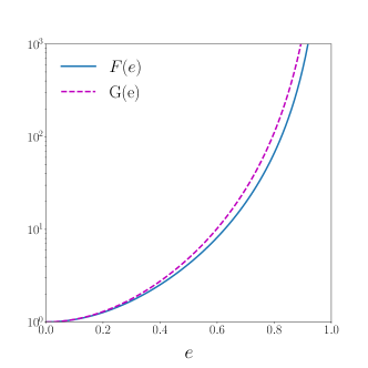
Figure 1: Eccentricity functions $F(e)$ and $G(e)$, defined in Eq. (11) and Eq. (15), respectively.

Quite a few factors affect the observed $\dot{P}_{b}$ (denoted as $\dot{P}_{b}^{\rm obs}$), including the relative acceleration between the binary pulsar and the Solar System barycenter, the kinematic effects, and so on (see Ref. Lorimer and Kramer (2005) for a detailed account). In our study the theoretical $\dot{P}_{b}$ (including the quadrupole radation in GR and the contribution from the massive graviton) should be compared to the intrinsic orbital decay rate of binary pulsar systems. We should subtract other effects from the observed orbital period decay Shklovskii (1970); Damour and Taylor (1991), to obtain the intrinsic orbital decay,

$$\dot{P}_{b}^{\rm intr}=\dot{P}_{b}^{\rm obs}-\dot{P}_{b}^{\rm Acc}-\dot{P}_{b}^{\rm Shk},$$ (17)

where $\dot{P}_{b}^{\rm Acc}$ is caused by the difference of accelerations of binary pulsars and the Solar System projected along the line of sight to the pulsar; $\dot{P}_{b}^{\rm Shk}$ is the “Shklovskii” effect Shklovskii (1970) caused by the relative kinematic motions of the binary pulsar with respect to the Solar System barycenter.

III.2 Individual bounds on the graviton mass

From above descriptions, we can use the fractional discrepancy $\Delta$ of binary pulsars to get an individual limit on the graviton mass per pulsar. We assume the measured discrepancy $\Delta$ to be normally distributed about its unknown actual value Finn and Sutton (2002). The 1-$\sigma$ uncertainty in $\Delta$ (see Table 1) is of the same order as the central value, so it must be properly accounted for in the analysis. The squared mass of graviton must be non-negative, but the standard confidence belts can not guarantee to always give $\Delta$ a physical interval Feldman and Cousins (1998). As discussed above we choose an ordering principle to specify uniquely the acceptance intervals which can avoid unphysical results. Using Table X in Ref. Feldman and Cousins (1998), we choose the $90\%$ C.L. confidence intervals which are obtained by an ordering principle to replace the standard confidence intervals.

We carefully choose 9 binary pulsars, and use the parameters in Table 1 and Eq. (16) to calculate the $90\%$ C.L. upper limit on the graviton mass bound individually. The relevant parameters of 9 binary pulsars are listed in Table 1, and our results are listed in Table 2. The bounds in Table 2 are sorted by the strength in constraining $m_{g}$. We notice that the updated parameters of PSRs B1913+16 and B1534+12 give tighter mass bounds than the widely used mass bound in Ref. Finn and Sutton (2002). This is because of longer observational span and higher quality of timing data. The best single limit on the graviton mass comes from the Hulse-Taylor pulsar PSR B1913+16, which gives,

$$m_{g}<3.5\times 10^{-20}\,{\rm eV}/c^{2}\quad\mbox{(90\% C.L.)}\,.$$ (18)

It improves the previous limit from this pulsar (see Table I in Ref. Finn and Sutton (2002)) by a factor of three.

Table 2: The mass bounds from individual binary pulsar systems at $90\%$ C.L., sorted by their constraints on $m_{g}$.

PSR	Graviton mass upper bound
B1913+16	$3.5\times 10^{-20}\,{\rm eV}/c^{2}$
J0737$-$3039	$4.3\times 10^{-20}\,{\rm eV}/c^{2}$
B1534+12	$5.2\times 10^{-20}\,{\rm eV}/c^{2}$
J1738+0333	$1.1\times 10^{-19}\,{\rm eV}/c^{2}$
J2222$-$0137	$1.8\times 10^{-19}\,{\rm eV}/c^{2}$
J1909$-$3744	$2.2\times 10^{-19}\,{\rm eV}/c^{2}$
J1012+5307	$2.9\times 10^{-19}\,{\rm eV}/c^{2}$
J1713+0747	$3.0\times 10^{-19}\,{\rm eV}/c^{2}$
J0348+0432	$6.0\times 10^{-19}\,{\rm eV}/c^{2}$

III.3 A combined bound on the graviton mass

We use Bayesian statistics to combine the information from observations of several pulsar systems, and utilize the relevant parameters of 9 binary pulsars in Table 1 to give a combined bound on the graviton mass. There are no unknown parameters $\bm{\Xi}$ in this study, so we can rewrite Eq. (12) to,

$$P\left(\left.m_{g}\right|{\cal D},{\cal H},{\cal I}\right) =\frac{P\left(\left.{\cal D}\right|m_{g},{\cal H},{\cal I}\right)P\left(\left.m_{g}\right|{\cal H},{\cal I}\right)}{P\left(\left.{\cal D}\right|{\cal H},{\cal I}\right)}\,.$$ (19)

We assume that the observations of different binary pulsars are statistically independent, so the combined likelihood can be split into the product of multiple individual likelihoods,

$$P\left(\left.{\cal D}\right|m_{g},{\cal H},{\cal I}\right)=\prod^{n}_{i=1}P\left(\left.{\cal D}_{i}\right|m_{g},{\cal H},{\cal I}\right)\,,$$ (20)

where $n$ is the number of binary pulsars. To be more explicit, we choose the individual likelihood,

$$P\left(\left.{\cal D}_{i}\right|m_{g},{\cal H},{\cal I}\right)\propto{\rm exp}\left[-\frac{1}{2}\frac{\left(\dot{P}^{m_{g}}_{b}+\dot{P}^{\rm GR}_{b}-\dot{P}_{b}^{\rm intr}\right)^{2}}{\sigma^{2}}\right]\,,$$ (21)

where $\sigma$ is total uncertainty including the observational uncertainty and the modeling uncertainty from $\dot{P}_{b}^{\rm Acc}$, $\dot{P}_{b}^{\rm Shk}$, and so on; see Eq. (17); $\dot{P}^{m_{g}}_{b}$ is the possible contribution from a nonzero graviton mass,

$$\dot{P}^{m_{g}}_{b}\equiv\dot{P}_{b}-\dot{P}^{\rm GR}_{b}=\frac{5}{24}m_{g}^{2}\left(\frac{c^{2}P_{b}}{2\pi\hbar}\right)^{2}\frac{1}{F(e)}\dot{P}^{\rm GR}_{b}\,.$$ (22)

For the prior probability of the graviton mass, we use two un-informative choices in this paper. One is to choose a uniform prior probability in $m_{g}$, and the other is to choose a uniform prior probability in $\ln m_{g}$. For both prior probabilities, we take the graviton mass in the range $m_{g}\in\left[10^{-26},10^{-16}\right]\,{\rm eV}/c^{2}$. For ease in comparison, the range of prior is the same as that chosen by the LIGO/Virgo Collaboration Abbott et al. (2016).

In Eq. (19), we use the relevant parameters of binary pulsars in Table 1 and our two different prior distributions to give two different posterior distributions. The posteriors are shown in Fig. 2. Because the prior uniform in $\ln m_{g}$ gives more support to a smaller mass, overall it gives a better constraint in $m_{g}$. The apparent drop in the posterior distribution, when the prior uniform in $m_{g}$ is used, is artificial in Fig. 2 due to the usage of a logarithmic scale in the abscissa axis.

We calculate the upper limit on the graviton mass from two posterior distributions. When the prior is uniform in $m_{g}$, we have,

$$m_{g}<3.1\times 10^{-20}\,{\rm eV}/c^{2}\quad\mbox{(90\% C.L.)}\,.$$ (23)

As one can see, this result is very close to the limit from the Hulse-Taylor pulsar PSR B1913+16 in the frequentist approach (see Table 2).

When the prior is uniform in $\ln m_{g}$, we have,

$$m_{g}<5.2\times 10^{-21}\,{\rm eV}/c^{2}\quad\mbox{(90\% C.L.)}\,.$$ (24)

This limit, though not as tight as some other limits de Rham et al. (2017), improves the Finn-Sutton limit in 2002 Finn and Sutton (2002) by a factor of more than 10.

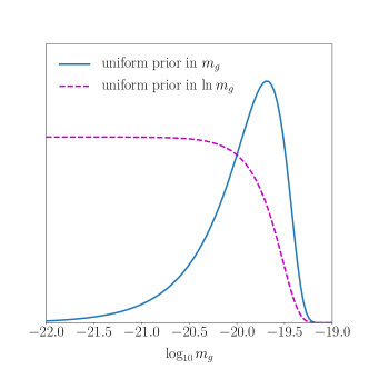
Figure 2: The posterior distributions with two different priors for $m_{g}$.

IV Discussions

During recent decades, because of the tremendous advance in constructing theories for massive gravity Dvali et al. (2000); de Rham and Gabadadze (2010); de Rham et al. (2011); Hassan and Rosen (2012); de Rham (2014); de Rham et al. (2017), there are various means to give graviton mass bounds, which generally can be classified into three categories de Rham et al. (2017). We briefly list them below, and compare them with our results in the following.

1. If the graviton is a massive boson, the gravitational force typically acquires an exponential Yukawa suppression, and the static gravitational potential is modified to $\Phi\propto e^{-m_{g}r}/r$. It is different from the case of massless gauge bosons where the potential has a $1/r$ falloff Will (2018).

2. If gravity is propagated by a massive field, the massive graviton propagator will lead to a modified dispersion relation $E^{2}=p^{2}c^{2}+m_{g}^{2}c^{4}$. The direct result is that GWs no longer travel at the velocity of light but depend on their frequencies Will (1998).

3. For a spin-2 massive boson, there may be five degrees of freedom in the propagation, including two tensor modes, two vector modes, and one scalar mode. The extra modes could lead to a fifth force de Rham et al. (2017).

The above three arguments are not always true in specific massive gravity theories, e.g. in the DGP model Dvali et al. (2000) and the dRGT theory de Rham et al. (2011) where screening mechanisms take effect Vainshtein (1972). Nevertheless, they are effective in communicating information in the community as simple phenomenological treatments.

Our limit obtained in this paper is also a phenomenological one based on the phenomenological action (7) Visser (1998); Finn and Sutton (2002). Below, we compare our result with those existing in the literature.

For Yukawa potential, the falloff is obvious when the distance from the source is greater than the Compton wavelength of graviton, $\lambda_{g}\equiv h/m_{g}c$. The most recent mass bound from ephemeris observations of the Solar System is $m_{g}<(6-10)\times 10^{-24}\,{\rm eV}/c^{2}$ Will (2018). This result is three orders of magnitude better than our result in Eq. (24). However, our mass bound comes from a dynamical process and can reflect the dynamics of binaries. The Yukawa potential describes a static field, and though the result from Yukawa potential is more competitive, it can not reflect two-body dynamics.

Modified dispersion relation is based on the linearized theory of gravity, which is similar to the Yukawa potential. The frequency of GWs is increasing during the binary inspiral. If graviton is massive, according to its modified dispersion relation the velocity of graviton should depend on the GW frequency Will (1998). It means that the lower-frequency GWs, which are emitted earlier, propagate slower than the higher-frequency GWs which are emitted later. The different propagating velocities would distort the shape of the observed GW waveforms Will (1998). So one can get the mass bounds from the GW detection, as were done by the LIGO/Virgo Collaboration Abbott et al. (2016, 2017, 2019) (see Sec. I). Compared with our result, the limit from GWs is more competitive. However, the mass bound coming from the direct detection of GWs is an effect of accumulation in GW phases. It is of different nature to the limit from binary pulsars which reflects a dynamical process of a binary motion. These two kinds of limits are of a kinematic origin for GWs and of a dynamic origin for binary pulsars.

For the fifth force, the bounds on the graviton mass come from the additional modes. In general, studies focus on the scalar mode and neglect the vector modes. Although the vector modes can induce a fifth force in principle, they usually do not couple to matter in the decoupling limit de Rham et al. (2017). The Finn-Sutton method focuses on the two transverse tensor modes only, which is different from the fifth force. The mass bounds from the fifth force are tightest, such as the ones from the lunar laser ranging experiments in the DGP model Dvali et al. (2000) which is $m_{g}<10^{-32}\,{\rm eV}/c^{2}$ Dvali et al. (2003). But these bounds are model dependent, such as for the DGP model and the dRGT theory de Rham and Gabadadze (2010); de Rham et al. (2011). In comparison, we consider our limit much more model-independent.

Our limit in Eq. (24) from binary pulsars is not as tight as the other results, but it is the only dynamical bound which comes from binary pulsars (see however, Refs. de Rham et al. (2013a, b)). We consider it complementary to bounds from other means (also complementary to the limits from binary pulsars in a model-specific treatment). In the future, we can improve the binary pulsar measurements and achieve smaller uncertainties on the timing parameters with the Five-hundred-meter Aperture Spherical Telescope (FAST) and the Square Kilometre Array Kramer et al. (2004); Shao et al. (2015); Bull et al. (2018). Especially, the observed timing precision on the $\dot{P}_{b}$ is proportional to $T^{-5/2}$ where $T$ is the observational span. Therefore, if we can model the Milky Way accurately to account for the extra contributions in $\dot{P}_{b}^{\rm obs}$ [see Eq. (17)], the limit from the Finn-Sutton method improves quickly. Then we will get a tighter mass bound on graviton in a dynamic regime with binary pulsars.

Finally, as was pointed out in Sec. II.1, we would like to stress that, same as the well-recognized limit from Finn and Sutton (2002), our limits are based on the phenomenological action (7). It is a phenomenological treatment of a linearized version of a massive rank-2 tensor field $g_{\mu\nu}$; it should not be taken as a full and sophisticatedly designed theory. The behavior of the tensor modes is the same as that in a healthy theory of massive gravity and the bound which comes from the Finn-Sutton method is in principle applicable to binary pulsar systems de Rham et al. (2017). This viewpoint also applies to the limits obtained from the propagation of GWs and the Yukawa potential. These generic limits do not necessarily mean that they are applicable to all theories of massive gravity de Rham (2014); de Rham et al. (2017). Nevertheless, they are still useful as simple empirical results on the mass of graviton.