Wasserstein Style Transfer

Abstract

We propose Gaussian optimal transport for Image style transfer in an Encoder/Decoder framework . Optimal transport for Gaussian measures has closed forms Monge mappings from source to target distributions. Moreover interpolates between a content and a style image can be seen as geodesics in the Wasserstein Geometry. Using this insight, we show how to mix different target styles , using Wasserstein barycenter of Gaussian measures. Since Gaussians are closed under Wasserstein barycenter, this allows us a simple style transfer and style mixing and interpolation. Moreover we show how mixing different styles can be achieved using other geodesic metrics between gaussians such as the Fisher Rao metric, while the transport of the content to the new interpolate style is still performed with Gaussian OT maps. Our simple methodology allows to generate new stylized content interpolating between many artistic styles. The metric used in the interpolation results in different stylizations.

1 Introduction

Image style transfer consists in the task of modifying an image in a way that preserves its content and matches the artistic style of a target image or a collection of images. Defining a loss function that captures this content/style constraint is challenging. A big progress in this field was made since the introduction of the neural style transfer in the seminal work of Gatys et al [1, 2]. Gatys et al showed that by matching statistics of the spatial distribution of images in the feature space of deep convolutional neural networks (spatial Grammian), one could define a style loss function. In Gatys et al method, the image is updated via an optimization process to minimize this “network loss". One shortcoming of this approach is that is slow and that it requires an optimization per content and per style images. Many workarounds have been introduced to speedup this process via feedforward networks optimization that produce stylizations in a single forward pass [3, 4, 5, 6]. Nevertheless this approach was still limited to a single style image. [7] introduced Instance Normalization (IN) to improve quality and diversity of stylization. Multiple styles neural transfer was then introduced in [8] thanks to Conditional Instance Normalization (CIN). CIN adapts the normalized statistics of the transposed convolutional layers in the feedforward network with learned scaling and biases for each style image for a fixed number of style images. The concept of layer swap in [9] resulted in one of the first arbitrary style transfer. Adaptive instance Normalization was introduced in [10] by making CIN scaling and biases learned functions from the style image, which enabled also arbitrary style transfer . The Whitening Coloring Transform (WCT) [11] which we discuss in details in Section 2 developed a simple framework for arbitrary style transfer using an Encoder/Decoder framework and operate a simple normalization transform (WCT) in the encoder feature space to perform the style transfer.

Our work is the closest to the WCT transform, where we start by noticing that instance normalization layers (IN,CIN, adaIN and WCT) are performing a transport map from the spatial distribution of a content image to the one of a style image, and the implicit assumption in deriving those maps is the Gaussianity of the spatial distribution of images in a deep CNN feature space. The Wasserstein geometry of Gaussian measures is very well studied in optimal transport [12] and Gaussian Optimal Transport (OT) maps have closed forms. We show in Section 3 that those normalization transforms are approximations of the OT maps. Linear interpolations of different content or styles at the level of those normalization feature transforms have been successfully applied in [10, 8] we show in Section 4 that this can be interpreted and improved as Gaussian geodesics in the Wasserstein geometry . Furthermore using this insight, we show in Section 5 that we can define novel styles using Wasserstein barycenyter of Gaussians [13]. We also extend this to other Fréchet means in order to study the impact of the ground metric used on the covariances in the novel style obtained via this non linear interpolation. Experiments are presented in Section 7.

2 Universal Style Transfer

We review in this Section the approach of universal style transfer of WCT [11].

Encoding Map. Given a content image $I_{c}$ and a style image $I_{s}$ and a Feature extractor $F_{j}:\mathbb{R}^{d}\to\mathbb{R}^{m},j=1\dots n,$ where $n$ is the spatial output of $F$, $m$ is its feature dimension . Define the following Encoding map: $\bm{E}:\leavevmode\nobreak\ \mathbb{R}^{d}\to\mathscr{P}(\mathbb{R}^{m}):\leavevmode\nobreak\ \leavevmode\nobreak\ I\to\nu_{I}=\frac{1}{n}\sum_{j=1}^{n}\delta_{F_{j}(I)},$ where $\mathscr{P}(\mathbb{R}^{m})$ is the space of empirical measures on $\mathbb{R}^{m}$. For example $F$ is a VGG [14] CNN that maps an image to $\mathbb{R}^{C\times(H\times W)}$($C$ is the number of channels, $H$ the height and $W$ the width). In other words the CNN defines a distribution in the space of dimension $m=C$, and we are given $n=C\times H$ samples of this distribution. We note $\nu=\bf{E}(I)$ this empirical distribution, i.e the spatial distribution of image $I_{c}$ in the feature space of a deep convolutional network $F$.

Decoding Map. We assume that the encoding $\bf{E}$ is invertible , i.e exists: $\bm{D}:\leavevmode\nobreak\ \mathscr{P}(\mathbb{R}^{m})\to\mathbb{R}^{d}:\leavevmode\nobreak\ \leavevmode\nobreak\ \nu\to\bf{D}(\nu),$ such that $\bm{D}(\bm{E}(I))=I$. $\bm{(E,D)}$ is a VGG image Encoder/ Decoder for instance trained from the pixel domain to a spatial convolutional layer output in VGG and vice-versa.

Universal Style Transfer in Feature Space. Universal style transfer approach [11] works in the following way: WCT (Whitening Coloring Transform) defines a transform $\bm{T}_{c\to s}$ (we will elaborate later on this transform) in the feature space $\mathbb{R}^{m}$: $\bm{T}_{c\to s}:\leavevmode\nobreak\ \mathbb{R}^{m}\to\mathbb{R}^{m}:\leavevmode\nobreak\ \leavevmode\nobreak\ x\to\bm{T}_{c\to s}(x),$ the style transfer Transform $\bm{T}_{c\to s}$ operates in the feature space and defines naturally a push forward map on the spatial distribution of the features of content image $I_{c}$:

$$\bm{T}_{c\to s,\#}(\nu(I_{c})):=\frac{1}{n}\sum_{j=1}^{n}\delta_{\bm{T}_{c\to s}(F_{j}(I_{c}))}.$$

$\bm{T}_{c\to s}$ is defined so that the style transfer happens in the feature space i.e $\bm{T}_{c\to s,\#}(\nu(I_{c}))=\nu(I_{s})$. We obtain the stylized image $\tilde{I}_{c\to s}$ by decoding back to the image domain :

$$\tilde{I}_{c\to s}=\bm{D}({\color[rgb]{0,0,1}\bm{T}}_{c\to s,\#}(\bm{E}(I_{c}))).$$

From this formalism we see that the universal style transfer problem amounts to finding a transport map $\bm{T}_{c\to s}$ from the spatial distribution of a content image in a feature space $\nu(I_{c})$ to the the spatial distribution of a target image in the same feature space $\nu(I_{s})$. We show in the next section how to leverage optimal transport theory to define such maps. Moreover we show that the WCT transform and Adaptive instance normalization are approximations to the optimal transport maps.

3 Wasserstein Universal Style Transfer

Given $\nu_{c}=\bm{E}(I_{c})$ and $\nu_{s}=\bm{E}(I_{s})$, we formulate the style transfer problem as finding an optimal Monge map:

$$\inf_{T}\int\left\lVert{x-T(x)}\right\rVert^{2}_{2}d\nu_{c}(x),\text{such that }T_{\#}(\nu_{c})=\nu_{s}$$ (1)

the optimal value of this problem is $W^{2}_{2}(\nu_{c},\nu_{s})$, the Wasserstein two distance between $\nu_{c}$ and $\nu_{s}$. Under some regularity conditions on the distributions, the optimal transport exists and is unique and $T_{c\to s}$ is the gradient of a convex potential [15]

Wasserstein Geometry of Gaussian Measures. Computationally Problem (1) can be solved using for example entropic regularization of the equivalent Kantorovich form of $W^{2}_{2}$ [16, 17] or in an end to end approach using automatic differentiation of a Sinkhorn loss [18, 19] . We take here another route, using the following known fact that Gaussian measures OT provides a lower bound on the Wasserstein distance [20] . For any two measures $\mu$ and $\nu$:

$$W^{2}_{2}(\mu,\nu) \geq W^{2}_{2}(\pazocal{N}(m_{\mu},\Sigma_{\mu}),\pazocal{N}(m_{\nu},\Sigma_{\nu}))$$

where $m_{\mu},\Sigma_{\mu}$ are means and covariance of $\mu$, and $m_{\nu},\Sigma_{\nu}$ of $\nu$. The Wasserstein geometry of Gaussian measures is well studied and have many convenient computational properties [12], we summarize them in the following:

1) Closed Form $W^{2}_{2}$. Given two Gaussians distributions $\nu=\pazocal{N}(m_{\mu},\Sigma_{\mu})$, and $\mu=\pazocal{N}(m_{\nu},\Sigma_{\nu})$ we have:

$$W^{2}_{2}(\pazocal{N}(m_{\mu},\Sigma_{\mu}),\pazocal{N}(m_{\nu},\Sigma_{\nu}))=\left|\left|m_{\nu}-m_{\nu}\right|\right|^{2}+d^{2}_{\mathscr{B}}(\Sigma_{\mu},\Sigma_{\nu}),$$

where

$$d^{2}_{\mathscr{B}}(\Sigma_{\mu},\Sigma_{\nu})=\text{trace}\left(\Sigma_{\mu}+\Sigma_{\nu}-2\left(\Sigma^{\frac{1}{2}}_{\mu}\Sigma_{\nu}\Sigma^{\frac{1}{2}}_{\mu}\right)^{\frac{1}{2}}\right)$$

is the Bures metric between covariances. The Bures metric is a goedesic metric on the PSD cone. (In Section 5.2 we discuss properties of this metric).

2) Closed Form Monge Map. The optimal transport map between two Gaussians with non degenerate covariances (full rank ) has a closed form: $T_{\mu\to\nu}:x\to m_{\nu}+A(x-m_{\mu}),$ where $A=\Sigma^{-\frac{1}{2}}_{\mu}\left(\Sigma^{\frac{1}{2}}_{\mu}\Sigma_{\nu}\Sigma^{\frac{1}{2}}_{\mu}\right)^{\frac{1}{2}}\Sigma^{-\frac{1}{2}}_{\mu}=A^{\top},$ i.e $T_{\mu\to\nu,\#}(\mu)=\nu$ and $T_{\mu\to\nu}$ is optimal in the $W^{2}_{2}$ sense. If the Gaussian were degenerate we can replace the square root matrices inverses with pseudo-inverses [21].

Gaussian Wasserstein Style Transfer. The spatial distribution of images in CNN feature space is not exactly Gaussian, but instead of having the solve Problem (1) we can use the Gaussian lower bound and obtain a closed form optimal map from the content distribution to the style distribution as follows:

$$\boxed{\bm{T^{\pazocal{W}}}_{\nu_{c}\to\nu_{s}}(x)=\mu_{s}+A_{c\to s}(x-\mu_{c}),}$$ (2)

where $\mu_{c}=\frac{1}{n}\sum_{j=1}^{n}F_{j}(I_{c}),\mu_{s}=\frac{1}{n}\sum_{j=1}^{n}F_{j}(I_{s})$ , and $\Sigma_{c}=\frac{1}{n}\sum_{j=1}^{n}(F_{j}(I_{c})-\mu_{c})(F_{j}(I_{c})-\mu_{c})^{\top}$, and $\Sigma_{s}=\frac{1}{n}\sum_{j=1}^{n}(F_{j}(I_{s})-\mu_{s})(F_{j}(I_{s})-\mu_{s})^{\top}$ are means and covariances of $\nu_{c}$ and $\nu_{s}$ resp. and

$$A_{c\to s}=\Sigma^{-\frac{1}{2}}_{c}\left(\Sigma^{\frac{1}{2}}_{c}\Sigma_{s}\Sigma^{\frac{1}{2}}_{c}\right)^{\frac{1}{2}}\Sigma^{-\frac{1}{2}}_{c}.$$

Finally the Universal Wasserstein Style Transfer can be written in the following compact way, that is summarized in Figure 1:

$$\boxed{\tilde{I}_{c\to s}=\bm{D}({\color[rgb]{0,0,1}\bm{T}^{\pazocal{W}}}_{\nu_{c}\to\nu_{s},\#}(\bm{E}(I_{c}))).}$$ (3)

Figure 1: Wasserstein Style Transfer

Relation to WCT and to Adaptive Instance Normalization. We consider two particular cases:
1) Commuting covariances and WCT [11]. Assuming that the covariances $\Sigma_{c}$ and $\Sigma_{s}$ commute meaning that $\Sigma_{c}\Sigma_{s}=\Sigma_{s}\Sigma_{c}$ ($\Sigma_{s}$ and $\Sigma_{c}$ have a common orthonormal basis ) it is easy to see that the optimal transport map reduces to :

$$\bm{T^{\pazocal{W}}}_{\nu_{c}\to\nu_{s}}(x)=\mu_{s}+\Sigma_{s}^{\frac{1}{2}}\Sigma^{-\frac{1}{2}}_{c}(x-\mu_{c})=\bm{T}^{\text{WCT}}_{c\to s}(x)$$

which is exactly the Whitening and Coloring Transform (WCT). Hence we see that WCT [11] is only optimal when the covariances commute (a particular case is diagonal covariances).

2) Diagonal Covriances and AdaIN, Instance Normalization (IN) and Conditional Instance Normalization (CIN)[10, 7, 8]. Let $\sigma_{s}$ be the diagonal of $\Sigma_{s}$ and $\sigma_{c}$ be the diagonal of $\Sigma_{c}$. In case the covariances were diagonal it is easy to see that:

$$\bm{T^{\pazocal{W}}}_{\nu_{c}\to\nu_{s}}(x)=\mu_{s}+\sqrt{\sigma_{s}}\odot\frac{(x-\mu_{c})}{\sqrt{\sigma_{c}}}=\text{AdaIN}(x),$$

this is exactly the expression of adaptive instance normalization AdaIN. We conclude that AdaIN, IN and CIN implement a diagonal approximation of the optimal Gaussian transport map ($(\mu_{s},\sigma_{s})$, are learned constant scaling and biases in IN and CIN , and are adaptive in adaIN).

4 Wasserstein Style/Content Interpolation with McCann Interpolates

One shortcoming of the formulation in problem (1) is that it does not allow to balance the content/style preservation as it is the case in end to end style transfer. Let $t\in[0,1]$ we formulate the style transfer problem with content preservation as follows:

$$\min_{\nu}(1-t)W^{2}_{2}(\nu,\nu_{c})+tW^{2}_{2}(\nu,\nu_{s}),$$ (4)

The first term in Equation (4) measure the usual "content loss" in style transfer and the second term measures the "style loss". $t$ balances the interpolation between the style and the content. In optimal transport theory, Problem (4) is known as the McCann interpolate [22] between $\nu_{c}$ and $\nu_{s}$ and the solution of (4) is a Wasserstein geodesic from $\nu_{c}$ to $\nu_{s}$ and is given by:

$$\nu_{t}=[(1-t)\text{Id}+tT_{\nu_{c}\to\nu_{s}}]_{\#}(\nu_{c})$$

The spatial distribution of images in CNN is not exactly Gaussian, but instead of having the solve Problem (4) we can again use the following Gaussian lower bound:

$$\min_{\nu\sim\pazocal{N}(\mu,\Sigma)}(1-t)W^{2}_{2}(\pazocal{N}(\mu,\Sigma),\pazocal{N}(\mu_{c},\Sigma_{c}))+tW^{2}_{2}(\pazocal{N}(\mu,\Sigma),\pazocal{N}(\mu_{s},\Sigma_{s})).$$ (5)

Fortunately this problem has also a closed form [22]:

$$\nu_{t}=\pazocal{N}(\mu_{t},\Sigma_{t})=[(1-t)\text{Id}+t\bm{T}^{\pazocal{W}}_{\nu_{c}\to\nu_{s}}]]_{\#}(\nu_{c}),$$

where $\bm{T}^{\pazocal{W}}_{\nu_{c}\to\nu_{s}}$ is given in Equation (2). $\{\nu_{t}\}_{t\in[0,1]}$ is a geodesic between $\nu_{c}$ and $\nu_{s}$. Finally the Wasserstein Style/Content Interpolation can be written in the following compact way:

$$\boxed{\nu_{t}=(1-t)\bm{E}(I_{c})+t{\color[rgb]{0,0,1}\bm{T}^{\pazocal{W}}}_{\nu_{c}\to\nu_{s},\#}(\bm{E}(I_{c})),\leavevmode\nobreak\ \leavevmode\nobreak\ \tilde{I}^{t}_{c\to s}=\bm{D}(\nu_{t}).}$$ (6)

In practice both WCT and AdaIN propose similar interpolations in feature space, we give here a formal justification for this approach. This formalism allows us to generalize to multiple styles interpolation using the Gaussian Wasserstein geometry of the spatial distribution of CNN images features.

5 Wasserstein Style Interpolation

Given $\{(I^{j}_{s},\lambda_{j})\}_{j=1\dots S}$, $S$ target styles images, and a content image $(I_{c},\lambda_{S+1})$,where $\lambda_{j}$ are interpolation factors such that $\sum_{j=1}^{S+1}\lambda_{j}=1$. A naive approach to content/$S$ styles interpolation can be given by:

$$\nu_{\lambda}=\sum_{j=1}^{S}\lambda_{j}\bm{T}^{\pazocal{W}}_{c\to s_{j},\#}(\bm{E}(I_{c}))+\lambda_{S+1}\bm{E}(I_{c}),\leavevmode\nobreak\ \leavevmode\nobreak\ I^{\lambda}_{s}=\bm{D}(\nu_{\lambda}),$$

this approach was proposed in both WCT and AdaIn by replacing $\bm{T}^{\pazocal{W}}$ by $T^{\text{WCT}}$ and AdaIN respectively. We show here how to define a non linear interpolation that exploits the Wasserstein geometry of Gaussian measures.

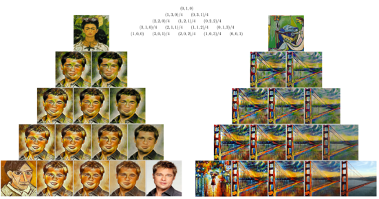
Figure 2: Wasserstein Barycenter Interpolation between a content image and two target styles images. The weights $\{\lambda_{j}\}$ used are given above the two examples.

5.1 Interpolation with Wasserstein Barycenters

Similarly to the content /style interpolation, we formulate the content / $S$ styles interpolation problem as a Wasserstein Barycenter problem [13] as follows. Let $\nu^{j}_{s}=\bm{E}(I^{j}_{s})$, and $\nu_{c}=\bm{E}(I_{c})$, we propose to solve the following Wasserstein Barycenter problem:

$$\nu^{s}_{\lambda}=\operatornamewithlimits{arg\,min}_{\nu}\sum_{j=1}^{S}\lambda_{j}W^{2}_{2}(\nu,\nu^{j}_{s})+\lambda_{S+1}W^{2}_{2}(\nu,\nu_{c})$$

and then find the optimal map from $\nu_{c}$ to the barycenter measure $\nu^{s}_{\lambda}$ $T_{\nu_{c}\to\nu^{s}_{\lambda}}.$ The final stylized image is obtained as follows: $\tilde{I}^{\lambda}_{s}=\bm{D}(\bm{T}_{\nu_{c}\to\nu^{s}_{\lambda}}(\bm{E}(I_{c}))).$

Again we resort to Gaussian optimal transport lower bound of the above problem:

$$\nu^{s}_{\lambda}=\operatornamewithlimits{arg\,min}_{\nu\sim\pazocal{N}(\mu,\Sigma)}\sum_{j=1}^{S}\lambda_{j}W^{2}_{2}(\pazocal{N}(\mu,\Sigma),\pazocal{N}(\mu^{j}_{s},\Sigma^{j}_{s}))+\lambda_{S+1}W^{2}_{2}(\pazocal{N}(\mu,\Sigma),\pazocal{N}(\mu_{c},\Sigma_{c})),$$ (7)

As shown by Agueh and Carlier [13] the Wasserstein Barycenter of Gaussians is itself a Gaussian $\nu^{s}_{\lambda}=\pazocal{N}(\bar{\mu}_{\lambda},\bar{\Sigma}_{\lambda}),$ where $\bar{\mu}_{\lambda}=\sum_{j=1}^{S}\mu^{s}_{j}+\lambda_{S+1}\mu_{c},$ and $\bar{\Sigma}_{\lambda}$ is a Bures Mean. Noting $\Sigma^{S+1}_{s}=\Sigma_{c}$ we have:

$$\bar{\Sigma}_{\lambda}=\operatornamewithlimits{arg\,min}_{\Sigma}\sum_{j=1}^{S+1}\lambda_{j}d^{2}_{\mathscr{B}}(\Sigma,\Sigma^{j}_{s})$$

Agueh and Carlier showed that $\bar{\Sigma}_{\lambda}$ is the unique positive definite matrix solution of the following fixed point problem: $\bar{\Sigma}_{\lambda}=\sum_{j=1}^{S+1}\lambda_{j}\left(\bar{\Sigma}^{\frac{1}{2}}\Sigma^{j}_{s}\bar{\Sigma}^{\frac{1}{2}}\right)^{\frac{1}{2}}.$ In order to solve this problem we use an alternative fixed point strategy proposed in [23], since it converges faster in practice:

$$\bar{\Sigma}_{\ell}=\sum_{j=1}^{S+1}\lambda_{j}\bar{\Sigma}_{\ell-1}^{-\frac{1}{2}}\left(\bar{\Sigma}^{\frac{1}{2}}_{\ell-1}\Sigma^{j}_{s}\bar{\Sigma}^{\frac{1}{2}}_{\ell-1}\right)^{\frac{1}{2}}\bar{\Sigma}_{\ell-1}^{-\frac{1}{2}},\ell=0\dots L-1,$$ (8)

and we initialized as in [21]: $\bar{\Sigma}_{0}=\Sigma^{j_{0}}_{s},j_{0}=\operatornamewithlimits{arg\,max}_{j=1\dots S+1}\lambda_{j},$ we found that $L=50$ was enough for convergence, i.e we set $\bar{\Sigma}_{\lambda}=\bar{\Sigma}_{L}$. Matrix square root and inverses were computed using SVD which gives an overall complexity of $O(Lm^{3})$ and we used truncated SVD to stabilize the inverses. Finally since the Barycenter is a Gaussian , the optimal transport map from the Gaussian spatial content distribution $\pazocal{N}(\mu_{c},\Sigma_{c})$ to the barycenter (mix of styles and content) $\pazocal{N}(\bar{\mu}_{\lambda},\bar{\Sigma}_{\lambda})$ is given in closed form as in Equation (2):

$$\boxed{\bm{T}^{\mathscr{W}}_{\nu_{c}\to\nu^{s}_{\lambda}}(x)=\bar{\mu}_{\lambda}+\Sigma^{-\frac{1}{2}}_{c}\left(\Sigma^{\frac{1}{2}}_{c}\bar{\Sigma}_{\lambda}\Sigma^{\frac{1}{2}}_{c}\right)^{\frac{1}{2}}\Sigma^{-\frac{1}{2}}_{c}.(x-\mu_{c})}.$$ (9)

Finally to obtain the stylized image as a result of targeting the mixed/style $\nu^{s}_{\lambda}$ we decode back:

$$\tilde{I}^{\lambda}_{cs}=\bm{D}(\bm{T}^{\mathscr{W}}_{\nu_{c}\to\nu^{s}_{\lambda}}(\nu_{c})).$$

Figure 2 gives an example of our approach for mixing content images with style images. We see that the Wasserstein barycenter captures not only the color distribution but also the details of the artistic style (for instance Frida Kahlo’s unibrow is well captured smoothly in the transition between Picasso self portrait and Frida Kahlo).

5.2 Style Interpolation with Fréchet Means

In the previous section we defined interpolations between the content and the styles images. In this section we define a "novel style" via an interpolation of style images only, we then map the content to the novel style using Gaussian optimal transport.

From Wasserstein Barycenter to Fréchet Means on the PSD manifold. As discussed earlier the Wasserstein Barycenter of the Gaussian approximations of the spatial distribution of style images in CNN feature spaces can be written as:

$$\min_{\mu,\Sigma}\sum_{j=1}^{S}\lambda_{j}\left(d^{2}_{\mu}(\mu,\mu^{j}_{s})+d^{2}_{\text{cov}}(\Sigma,\Sigma^{j}_{s})\right),$$ (10)

for $d^{2}_{\mu}(\mu,\mu^{\prime})=\left\lVert{\mu-\mu^{\prime}}\right\rVert^{2}_{2}$ the euclidean metric , $d^{2}_{cov}(\Sigma,\Sigma^{\prime})=d^{2}_{\mathscr{B}}(\Sigma,\Sigma^{\prime}),$ the Bures metric. The Bures Metric is a geodesic metric on the positive definite cone and and has another representation as a procrustes registration metric [24]:

$$d^{2}_{\mathscr{B}}(\Sigma,\Sigma^{\prime})=\min_{U\in\mathbb{R}^{m\times m},UU^{\top}=I}\left\lVert{\sqrt{\Sigma}-\sqrt{\Sigma^{\prime}}U}\right\rVert^{2}_{F}.$$

From this we see the advantage of Wasserstein barycenter on for example using $d^{2}_{\text{cov}}(\Sigma,\Sigma^{\prime})=\left\lVert{\Sigma-\Sigma^{\prime}}\right\rVert^{2}_{F}$ the Frobenius norm. Bures Metric aligns the the square root of covariances using a rotation. From this we see that by defining a new metric on covariances we can get different form of interpolates, we fix $d^{2}_{\mu}(\mu,\mu^{\prime})=\left\lVert{\mu-\mu^{\prime}}\right\rVert^{2}_{2}$, and hence on $\mu$ we use always the arithmetic mean $\mu_{arth}=\sum_{j=1}^{S}\lambda_{j}\mu^{j}_{s}$. We give here different metrics $d^{2}_{cov}$ that defines different Fréchet means on the PSD manifold (see [25] and references there in )

1) Arithmetic Mean: Solving Eq. (10) for $d^{2}_{\text{cov}}(\Sigma,\Sigma^{\prime})=\left\lVert{\Sigma-\Sigma^{\prime}}\right\rVert^{2}_{F}$, we define the target style $\nu^{\lambda,\text{arth}}_{s}=\pazocal{N}(\mu_{arth},\Sigma_{\text{arth}})$, where $\Sigma_{\text{arth}}=\sum_{j=1}^{S}\lambda_{j}\Sigma^{s}_{j}$.
2) Harmonic Mean: Solving Eq. (10) for $d^{2}_{\text{cov}}(\Sigma,\Sigma^{\prime})=\left\lVert{\Sigma^{-1}-\Sigma^{\prime-1}}\right\rVert^{2}_{F}$, we define the target style $\nu^{\lambda,\text{Harm}}_{s}=\pazocal{N}\left(\mu_{\text{arth}},\Sigma_{\text{Harm}}\right)$, where $\Sigma_{\text{Harm}}=\left(\sum_{j=1}^{S}\lambda_{j}(\Sigma^{s}_{j})^{-1}\right)^{-1}$.
3) Fisher Rao Mean (Karcher or Geometric Mean). For $d^{2}_{cov}(\Sigma,\Sigma^{\prime})=\left\lVert{\log(\Sigma^{-\frac{1}{2}}\Sigma^{\prime}\Sigma^{-\frac{1}{2}})}\right\rVert^{2}_{F}=2\mathscr{F}^{2}(\pazocal{N}(0,\Sigma),\pazocal{N}(0,\Sigma^{\prime})),$ that is the Riemannian natural metric or the Fisher Rao metric between Centered Gaussians. $\log$ here refers to matrix logarithm. The Fisher Rao metric is a geodesic distance and its metric tensor is the Fisher information matrix . Solving Eq. (10) with the Fisher Rao metric we obtain the so called Karcher Mean between PSD matrices $\Sigma_{\text{FisherRao}}$, and we define the target style $\nu^{\lambda,\text{FisherRao}}_{s}=\pazocal{N}\left(\mu_{\text{arth}},\Sigma_{\text{FisherRao}}\right)$.
In order to find the Karcher mean we use manifold optimization techniques of [26] as follows. The gradient manifold update is :

$$\Sigma_{\ell}=\Sigma^{\frac{1}{2}}_{\ell-1}\exp\left(-\eta\sum_{j=1}^{S}\log\left(\Sigma^{\frac{1}{2}}_{\ell-1}(\Sigma^{s}_{j})^{-1}\Sigma^{\frac{1}{2}}_{\ell-1}\right)\right)\Sigma^{\frac{1}{2}}_{\ell-1},$$ (11)

we initialize $\Sigma_{0}$ as in the Wasserstein case and iterate for $L=50$ iterations with $\eta$ the learning rate set to $0.01$.

Remark 1.

While we defined here the barycenter style of each metric as a Gaussian, Wasserstein Barycenter is the only one that guarantees a Gaussian barycenter [13].

Mapping a content image to a target novel style. Given now the new style $\nu^{\lambda,\text{mean}}_{s}$, where mean is in $\{\text{arth},\text{harm},\text{Fisher Rao},\text{Wasserstein}\}$, we stylize a content image $I_{c}$ using Gaussian Optimal transport as described in the paper:

$$\boxed{\tilde{I}_{c\to s}=\bm{D}({\color[rgb]{0,0,1}\bm{T}^{\pazocal{W}}}_{\nu_{c}\to\nu^{\lambda,\text{mean}}_{s},\#}(\bm{E}(I_{c}))).}$$

Our approach is summarized in Algorithms 1 and 2 given in Appendix.

6 Related works

OT for style Transfer and Image coloring. Color transfer between images using regularized optimal transport on the color distribution of images (RGB for example) was studied and applied in [27]. The color distribution is not gaussian and hence the OT problem has to be solved using regularization. Optimal transport for style transfer using the spatial distribution in the feature space of a deep CNN was also explored in [28, 29]. [28] uses $W^{2}_{2}$ for Gaussians as content and style loss and optimizes it in an end to end fashion similar to [1, 2]. [29] uses an approximation of the Wasserstein distance as a loss that is also optimized in an end to end fashion. Both approaches don’t allow universal style transfer and an optimization is needed for every style/content image pairs.

Wasserstein Barycenter for Texture Mixing. Similar to our approach for Wasserstein mixing in an encoder/decoder framework, [30] uses the wavelet transform to encode textures, applies Wasserstein barycenter on wavelets coefficients, and then decodes back using the inverse wavelet transform to synthesize a novel mixed texture. The wasserstein barycenter problem there has to be solved exactly and the Gaussian approximation can not be used since the wavelet coffecient distribution is not Gaussian. A special model for Gaussian texture mixing was developed in [21]. The advantage of using features of a CNN is that the Gaussian lower bound of the Wasserstein distance seems to be tight.

Other approaches to style Transfer. While our focus in this paper was on OT metrics for style transfer other approaches exist (see [31] for a review) and have used different type of losses such as MRF loss [32] , MMD loss [33], GAN loss [5] and cycle GAN loss [34].

7 Experiments

In order to test our approach of geometric mixing of styles we use the WCT framework [11], where we use a pyramid of $5$ encoders $(E_{r},D_{r}),r=1\dots 5$ at different spatial resolutions, where $(E_{5},D_{5})$ corresponds to the coarser resolution, and $(E_{1},D_{1})$ the finer resolution. Following WCT we use a coarse to fine approach to style transfer as follows. Given interpolation weights $\{\lambda_{j},j=1\dots S\}$, we start with $r=5$ and with $\nu_{c}=E_{5}(I_{c})$:

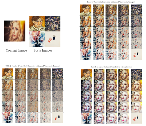
Figure 3: ( Table 1): Wasserstein Barycenter Interpolation between a content image given above and four target styles images given at the corner of the square. Each image in the square is for an interpolation weight $(\lambda_{1},\dots\lambda_{4})$, that are defined on a grid on the square. (Table 2): Fisher Rao Interpolation between the same content image given above and the same four target styles images given at the corner of the square. In both cases Gaussian Wasserstein transport plans are used to obtain the transformed image to the novel mixed style in the feature space, and the final image is obtained using the decoder. (Table 3): the AdaIn baseline that we showed that it does a diagonal approximation fails at capturing the subtle details of the style of the target images. Both Wasserstein and Fisher Rao approaches are successful, we notice that while Wasserstein barycenter is color dominant in defining the new style, the Fisher Rao barycenter capture more the strokes and captures better color variations in the novel artistic styles. We note that the Wasserstein is smoother as we change the interpolation weights then the Fisher Rao. (Figure is better seen in color and zooming in; See Appendix for a full resolution).

1. We encode all style images at resolution $r$, $E_{r}(I^{j}_{s}),j=1\dots s$. We define the mixed style $\nu^{\lambda,r}_{s}$ at resolution $r$ using one of the mixing strategies (Frechet Mean) in Section 4, using Algorithms 1 and 2.

2. We find the Wasserstein Transport map at resolution $r$ between the content $\nu_{c}$ and the novel style $\nu^{\lambda,r}_{s}$ and compute the transformed features: $\nu^{r}_{cs}=\bm{T}^{\pazocal{W}}_{\nu_{c}\to\nu^{\lambda,r}_{s},\#}(\nu_{c})$.

3. We decode the novel image at resolution $r$ : $I^{r}_{c}=D_{r}(\nu^{r}_{cs})$.

4. We set $\nu_{c}=E_{r-1}(I^{r}_{c})$, then set $r$ to $r-1$ and go to step $1$ until reaching $r=1$.

The stylized output of this procedure is $I^{1}_{c}$. We also experimented in the Appendix with applying the same approach but in fine to coarse way starting from the higher resolution $r=1$ to the lower resolution encoder $r=5$. We show in Figure 3 the output of our mixing strategy using two of the geodesic metrics namely Wasserstein and Fisher Rao barycenters. We give as baseline the AdaIn output for this (this same example was given in [10] we reproduce it using their available code). We show that using geodesic metrics to define the mixed style successfully capture the subtle details of different styles. More examples and comparison to literature and other types of mixing can be found in the Appendix.

8 Discussion and Conclusion

We conclude this paper by the following three observations on the spatial distribution of features in a deep convolutional neural network:

1. The success of Gaussian optimal transport between spatial distributions of deep CNN features that we demonstrated in this paper suggests that the network learned to "gaussianize" the space. Gaussinization [35] is a principle in unsupervised learning. It will be interesting to further study this Gaussianity hypothesis and to see if Gaussinization can be used as a regularizer for learning deep CNN or as an objective in self-supervised learning.

2. We showed that many of the spatial normalization layers used in deep learning such as Instance normalization [7] and related variants can be understood as approximations of Gaussian optimal transport. When used in an architecture between layers, the normalization layer acts like a transport map between the spatial distribution of consecutive layers. We hope this angle will help developing new normalization layers and a better understanding of the existing ones.

3. Geodesic metrics such as Wasserstein and the Fisher Rao metric allow better non linear interpolation in feature space.

Supplementary Material for Wasserstein Style Transfer

Appendix A Algorithms

Algorithm 1 Frechet Mean Style Interpolation and Content Stylization($d_{cov}$)

  Inputs: $\{I^{j}_{s}\}_{j=1\dots S}$ style images, content Image $I_{c}$ , interpolations weights $\{\lambda_{j}\}_{j=1\dots S+1}$, Encoder/Decoder $(\bm{E},\bm{D})$,.

  Encode: $\nu_{c}=\bm{E}(I_{c}),\nu^{j}_{s}=\bm{E}(I^{j}_{s}),j=1\dots S$

  Statistics: $(\mu_{c},\Sigma_{c}),(\mu^{j}_{s},\Sigma^{j}_{s}),j=1\dots S$

  Content/Style or Style only: if content/style $\mu^{s}_{S+1}=\mu_{c},\Sigma^{s}_{S+1}=\Sigma_{c},,S\leftarrow S+1$ , else pass.

  Target Bary Mean: $\bar{\mu}_{\lambda}=\sum_{j=1}^{S}\lambda_{j}\mu_{j}$.

  Target Bary Covariance: $\bar{\Sigma}_{\lambda}=$Frechet mean$(\{\lambda_{j},\Sigma^{j}_{s}\},d_{cov})$

  Novel Style: $\nu^{\lambda}_{s}=\pazocal{N}(\bar{\mu}_{\lambda},\bar{\Sigma}_{\lambda})$

  Gaussian OT Content to Target: Compute $\nu_{cs}=\bm{T}^{\mathscr{W}}_{\nu_{c}\to\nu^{s}_{\lambda},\#}(\nu_{c})$ given in Eq. (9)

  Decode: $\bm{D}(\nu_{cs})$

Algorithm 2 FRECHET MEAN($\{\lambda_{j},\Sigma^{j}_{s}\},d_{\text{cov}})$

  Initialize: $\bar{\Sigma}_{0}=\Sigma^{j_{0}}_{s},j_{0}=\operatornamewithlimits{arg\,max}_{j=1\dots S}\lambda_{j}$

  if $d_{cov}=d_{\text{Bures}}$ find $\bar{\Sigma}_{\lambda}$ solve using iterations in Eq (8)

  if $d_{cov}=d_{\text{Fisher Rao}}$ find $\bar{\Sigma}_{\lambda}$ solve using iterations in Eq (11)

  if $d_{cov}=d_{\text{Frobeinus}}$ $\bar{\Sigma}_{\lambda}=\sum_{j}\lambda_{j}\Sigma^{s}_{j}$

  if $d_{cov}=d_{\text{Harmonic}}$ $\bar{\Sigma}_{\lambda}=(\sum_{j}\lambda_{j}(\Sigma^{s}_{j})^{-1})^{-1}$

Appendix B Examples of Interpolating Content and Styles with Wasserstein Barycenter and Optimal Transport

In Figures 4, 5 ,6 we show examples of interpolations of content images with the style images. We used in this experiment a coarse to fine approach, i.e starting from matching upper layers of VGG to lower layers.

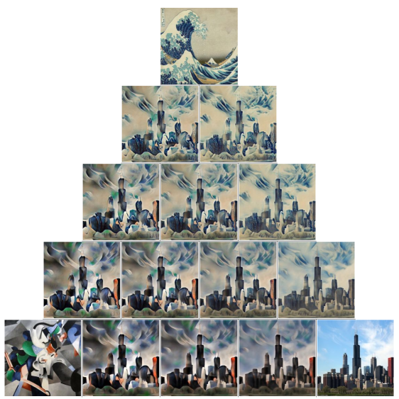
Figure 4: Wasserstein barycenters for Style Mixing and Transfer. The content image on the right corner of the triangle is mixed with the two styles images. Each image in the triangle correspond to a set of interpolation weights defined by proximity to the content or style images in the triangle.

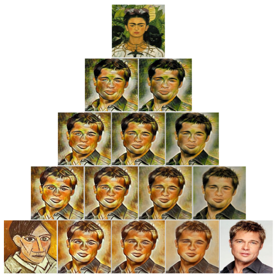
Figure 5: Wasserstein barycenters for Style Mixing and Transfer. The content image on the right corner of the triangle is mixed with the two styles images. Each image in the triangle correspond to a set of interpolation weights defined by proximity to the content or style images in the triangle.

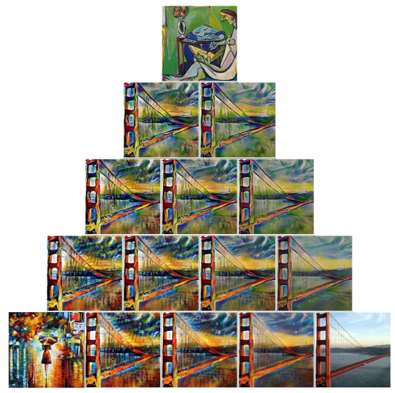
Figure 6: Wasserstein barycenters for Style Mixing and Transfer. The content image on the right corner of the triangle is mixed with the two styles images. Each image in the triangle correspond to a set of interpolation weights defined by proximity to the content or style images in the triangle.

Appendix C Mixing Styles with Frechet Means and Optimal Transport Style Transfer

Coarse to Fine.

-We give results of different Mixing strategies and a content stylization in a coarse to fine procedure as follows: Wasserstein Mixing in Table 8;Fisher Rao Mixing in Table 9 ;Arithmetic Mixing that would be close to WCT baseline [11] in Table 10; Harmonic Mixing in Table 11 ; AdaIN Mixing Table in 12. We also give another set of results on Wass Barycenter mixing in Table 15, Fisher Rao in Table 16 and AdaIn in 17

Fine to Coarse.

We experiment baselining WCT mixing [11] and Wasserstein Mixing in a Fine to coarse strategy (from lower layer to upper layers) results are given in Table 13 and Table 1.

Figure 7: Content Image. We give results of different Mixing strategies and a content stylization in a coarse to fine procedure as follows: Wasserstein Mixing in Table 8;Fisher Rao Mixing in Table 9 ;Arithmetic Mixing that would be close to WCT baseline [11] in Table 10; Harmonic Mixing in Table 11 ; AdaIN Mixing Table in 12; The style images are given on the four corners of each square.

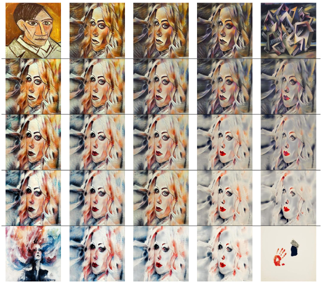
Figure 8: Coarse to Fine style Transfer: Content image is given in Figure 7. Wasserstein Barycenter Mixing of the styles (the four images in the corners of the square) and Wasserstein Transport of the content image to the novel style defined by the Wasserstein Barycenter for various interpolations weights. The stylized image is generated by following a coarse to fine scheme.

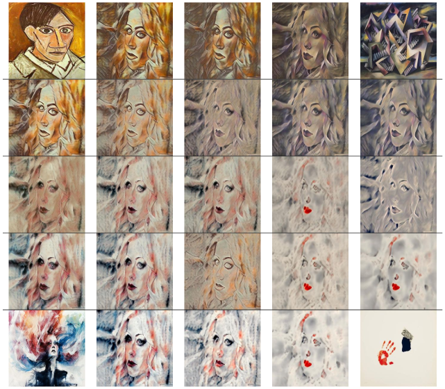
Figure 9: Coarse to Fine Generation: Karcher (Fisher Rao) Barycenter Mixing of the styles and Wasserstein Transport of the content image to the novel style defined by the Fisher Rao barycenter. The stylized is generated following a coarse to fine scheme.

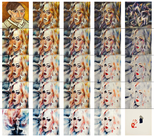
Figure 10: Coarse Fine Style Transfer: (Arithmetic )Euclidean Barycenter Mixing of Covariances and Wasserstein Transport. This is similar to a WCT type of mixing. The stylized image is similar to a Wasserstein Barycenter Mixing, nevertheless a closer look shows subtle differences. This hints to the fact the coarse layers are almost diagonal.

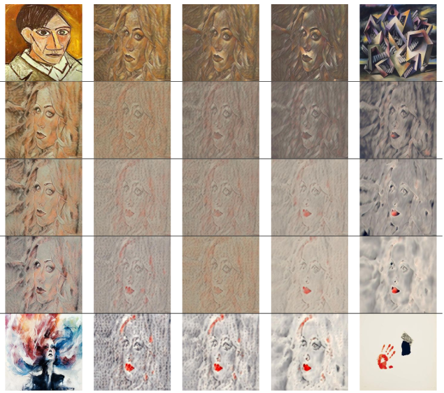
Figure 11: Coarse Fine Style Transfer: Harmonic Barycenter Mixing of Covariances and Wasserstein Transport. The Harmonic Mixing have saturation problems and does not produce good results.

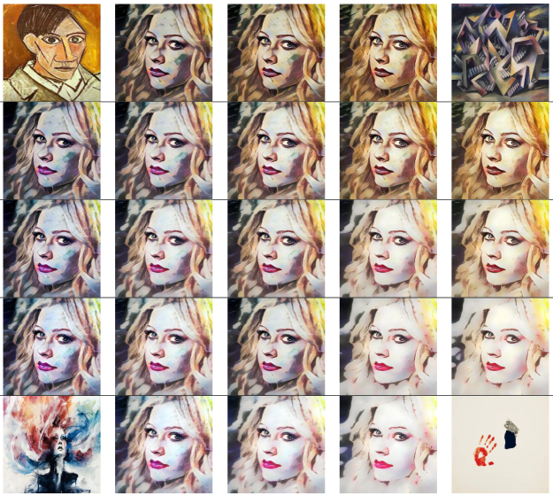
Figure 12: Adaptive Instance Normalization Mixing Baseline [10].

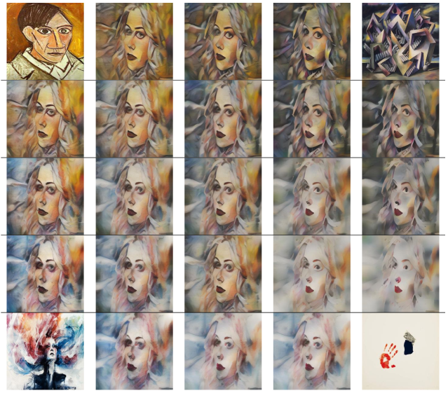
Figure 13: Fine to coarse style Transfer: Content image is given in Figure 7. Wasserstein Barycenter Mixing of the styles (the four images in the corners of the square) and Wasserstein Transport of the content image to the novel style defined by the Wasserstein Barycenter for various interpolations weights. The stylized image is generated by following a coarse to fine scheme.

Table 1: Fine to coarse style Transfer: Results of Arithmetic Mean Mixing (WCT Mixing [11]) , we see here that the coloring has a lot of black shadow over the face unlike the Wasserstein barycenter mixing approach, in the previous Table.

Figure 14: Content Image ( a Photo of Hotel Dieu painted by van gogh in the most right corner of the square). Stylization in mixture of four styles incluing van gogh painting are in Tables 15 for Wasserstein mixing and Table 16 for Fisher Rao Mixing. Table 17 is the AdaIN baseline.

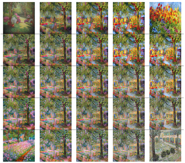
Figure 15: Coarse to Fine style transfer: Wasserstein Barycenter Mixing and Wasserstein Transport. The content image is given in Figure 14. The four styles are on the four corner of the square.

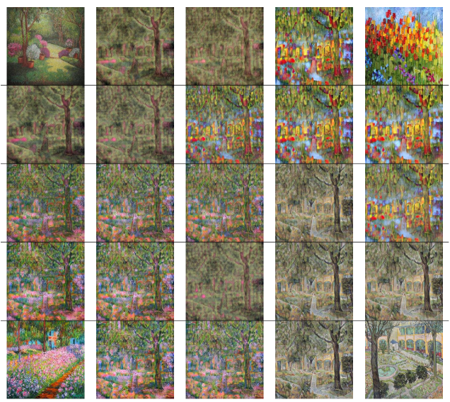
Figure 16: Coarse to fine style transfer: Fisher Rao Mixing and Wasserstein Transport.

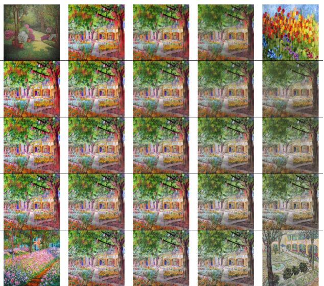
Figure 17: Adaptive Instance Normalization Mixing Baseline [10].

References

• [1] Leon A. Gatys, Alexander S. Ecker, and Matthias Bethge. Image style transfer using convolutional neural networks. In 2016 IEEE Conference on Computer Vision and Pattern Recognition, CVPR 2016, Las Vegas, NV, USA, June 27-30, 2016, 2016.
• [2] Leon A. Gatys, Alexander S. Ecker, Matthias Bethge, Aaron Hertzmann, and Eli Shechtman. Controlling perceptual factors in neural style transfer. In 2017 IEEE Conference on Computer Vision and Pattern Recognition, CVPR 2017, Honolulu, HI, USA, July 21-26, 2017, 2017.
• [3] Justin Johnson, Alexandre Alahi, and Li Fei-Fei. Perceptual losses for real-time style transfer and super-resolution. Lecture Notes in Computer Science, 2016.
• [4] Dmitry Ulyanov, Vadim Lebedev, Andrea Vedaldi, and Victor S. Lempitsky. Texture networks: Feed-forward synthesis of textures and stylized images. In ICML, 2016.
• [5] Chuan Li and Michael Wand. Precomputed real-time texture synthesis with markovian generative adversarial networks. In ECCV (3), 2016.
• [6] Xin Wang, Geoffrey Oxholm, Da Zhang, and Yuan-Fang Wang. Multimodal transfer: A hierarchical deep convolutional neural network for fast artistic style transfer. 2017 IEEE Conference on Computer Vision and Pattern Recognition (CVPR), 2017.
• [7] Dmitry Ulyanov, Andrea Vedaldi, and Victor Lempitsky. Improved texture networks: Maximizing quality and diversity in feed-forward stylization and texture synthesis. 2017 IEEE Conference on Computer Vision and Pattern Recognition (CVPR), 2017.
• [8] Vincent Dumoulin, Jonathon Shlens, and Manjunath Kudlur. A learned representation for artistic style. 2017.
• [9] Tian Qi Chen and Mark Schmidt. Fast patch-based style transfer of arbitrary style, 2016.
• [10] Xun Huang and Serge Belongie. Arbitrary style transfer in real-time with adaptive instance normalization. 2017 IEEE International Conference on Computer Vision (ICCV), 2017.
• [11] Yijun Li, Chen Fang, Jimei Yang, Zhaowen Wang, Xin Lu, and Ming-Hsuan Yang. Universal style transfer via feature transforms. In Advances in Neural Information Processing Systems 30. 2017.
• [12] Asuka Takatsu. Wasserstein geometry of gaussian measures. Osaka J. Math., 2011.
• [13] Martial Agueh and Guillaume Carlier. Barycenters in the wasserstein space. SIAM J. Math. Analysis, 43, 2011.
• [14] Karen Simonyan and Andrew Zisserman. Very deep convolutional networks for large-scale image recognition. CoRR arXiv:1409.1556, 2014.
• [15] Jean-David Benamou and Yann Brenier. A computational fluid mechanics solution to the Monge-Kantorovich mass transfer problem. Numerische Mathematik, 2000.
• [16] Marco Cuturi. Sinkhorn distances: Lightspeed computation of optimal transport. In Advances in neural information processing systems, pages 2292–2300, 2013.
• [17] Gabriel Peyré and Marco Cuturi. Computational optimal transport. Technical report, 2017.
• [18] Charlie Frogner, Chiyuan Zhang, Hossein Mobahi, Mauricio Araya, and Tomaso A Poggio. Learning with a wasserstein loss. In Advances in Neural Information Processing Systems, pages 2053–2061, 2015.
• [19] J. Feydy, T. Séjourné, F.-X. Vialard, S.-i. Amari, A. Trouvé, and G. Peyré. Interpolating between Optimal Transport and MMD using Sinkhorn Divergences. ArXiv e-prints, 2018.
• [20] J. A. Cuesta-Albertos, C. Matrán-Bea, and A. Tuero-Diaz. On lower bounds for thel2-wasserstein metric in a hilbert space. Journal of Theoretical Probability, 1996.
• [21] Gui-Song Xia, Sira Ferradans, Gabriel Peyré, and Jean-François Aujol. Synthesizing and mixing stationary gaussian texture models. SIAM J. Imaging Sciences, 2014.
• [22] Robert J. McCann. A convexity principle for interacting gases. Advances in Mathematics, 1997.
• [23] Pedro C. Álvarez Esteban, E. del Barrio, J.A. Cuesta-Albertos, and C. Matrán. A fixed-point approach to barycenters in wasserstein space. http://arxiv.org/pdf/1511.05355.
• [24] Valentina Masarotto, Victor M Panaretos, and Yoav Zemel. Procrustes metrics on covariance operators and optimal transportation of gaussian processes. Sankhya A, 2018.
• [25] Rajendra Bhatia. The Riemannian Mean of Positive Matrices. Springer Berlin Heidelberg, 2013.
• [26] Hongyi Zhang and Suvrit Sra. First-order methods for geodesically convex optimization. In COLT, 2016.
• [27] Sira Ferradans, Nicolas Papadakis, Julien Rabin, Gabriel Peyré, and Jean-Francois Aujol. Regularized discrete optimal transport. Scale Space and Variational Methods in Computer Vision, 2013.
• [28] Style transfer as optimal transport. https://github.com/VinceMarron/style_transfer.
• [29] Nicholas Kolkin, Jason Salavon, and Greg Shakhnarovich. Style transfer by relaxed optimal transport and self-similarity, 2019.
• [30] Julien Rabin, Gabriel Peyré, Julie Delon, and Marc Bernot. Wasserstein barycenter and its application to texture mixing. In Proceedings of the Third International Conference on Scale Space and Variational Methods in Computer Vision, SSVM’11, 2012.
• [31] Yongcheng Jing, Yezhou Yang, Zunlei Feng, Jingwen Ye, and Mingli Song. Neural style transfer: A review. CoRR.
• [32] Chuan Li and Michael Wand. Combining markov random fields and convolutional neural networks for image synthesis. 2016 IEEE Conference on Computer Vision and Pattern Recognition (CVPR), Jun 2016.
• [33] Yanghao Li, Naiyan Wang, Jiaying Liu, and Xiaodi Hou. Demystifying neural style transfer. Proceedings of the Twenty-Sixth International Joint Conference on Artificial Intelligence, 2017.
• [34] Jun-Yan Zhu, Taesung Park, Phillip Isola, and Alexei A Efros. Unpaired image-to-image translation using cycle-consistent adversarial networks. In Computer Vision (ICCV), 2017 IEEE International Conference on, 2017.
• [35] Scott Saobing Chen and Ramesh A. Gopinath. Gaussianization. In T. K. Leen, T. G. Dietterich, and V. Tresp, editors, Advances in Neural Information Processing Systems 13, pages 423–429. MIT Press, 2001.