Analytic crystals of solitons in the four dimensional
gauged non-linear sigma model

Abstract

The first analytic topologically non-trivial solutions in the (3+1)-dimensional gauged non-linear sigma model representing multi-solitons at finite volume with manifest ordered structures generating their own electromagnetic field are presented. The complete set of seven coupled non-linear field equations of the gauged non-linear sigma model together with the corresponding Maxwell equations are reduced in a self-consistent way to just one linear Schrodinger-like equation in two dimensions. The corresponding two dimensional periodic potential can be computed explicitly in terms of the solitons profile. The present construction keeps alive the topological charge of the gauged solitons. Both the energy density and the topological charge density are periodic and the positions of their peaks show a crystalline order. These solitons describe configurations in which (most of) the topological charge and total energy are concentrated within three-dimensional tube-shaped regions. The electric and magnetic fields vanish in the center of the tubes and take their maximum values on their surface while the electromagnetic current is contained within these tube-shaped regions. Electromagnetic perturbations of these families of gauged solitons are shortly discussed.

1 Introduction

One of the most relevant field theories (both due to its predictive power as well as its non-trivial topological features) is the non-linear sigma model. It is a very effective tool from high energy physics to statistical mechanics systems like quantum magnetism, the quantum hall effect, meson interactions, superfluid ³He and string theory (see [1] [2]). It was introduced in particle physics to describe the low-energy dynamics of pions (see for instance [3], [4] and references therein). On the other hand, as Skyrme noticed [5], such a theory does not possess solitonic solutions in flat, topologically trivial (3+1)-dimensional spacetimes. This can be shown using the Derrick’s scaling argument [6] (although Skyrme understood this before Derrick himself). That’s why Skyrme introduced his famous Skyrme term [5]. However, it is worth emphasizing that the beautiful currents-algebraic arguments by Witten [7] (see also [8], [9], [10] and references therein) to show that the solitons of this theory should be quantized at a semi-classical level as Fermions, and that such a theory describe the low-energy limit of QCD does not make explicit use of the Skyrme term itself but only of the fact that stable solitons with non-trivial third homotopy class exist (together with the well known Wess-Zumino-Witten term): a detailed review of these issues can be found in [2]. It is thus of great theoretical interest to search for a natural mechanism to avoid the Derrick scaling argument within the non-linear sigma model.

A topic which has a great theoretical as well as phenomenological importance is (a proper theoretical understanding of) crystals of solitons (which are very useful, for instance, in the description of cold and dense nuclear matter as a function of the topological charge [11], [12]). That’s why it is relevant to analyze configurations with many solitons coexisting within a fixed spatial volume. In this very interesting but extremely complicated phase the most common analytic methods are basically useless and so solitons living within a finite volume in (3+1)-dimensions with a finite topological charge are usually studied numerically. The importance of this issue comes from the fact that crystals of solitons are expected to appear when, within a fixed spatial volume, the topological charge is high enough. Until very recently, such solitonic crystals could only be found in two-dimensions (see [13], [14] and references therein). Powerful approximation schemes developed in [15], [16], [17], [18], [19], [20], [21], [22], shed light on many properties of these crystals but analytic examples are very rare.

It is well known that, as the density increases, quite complicated ordered structures denoted as nuclear pasta phases appear as well (see [23], [24], [25], [26] and references therein). The numerical works on these structures reveal the presence of “baryonic tubes” (nuclear spaghetti) in which most of the baryonic charge is concentrated within tube-shaped regions in three dimensions. These configurations with high topological charge living within finite volumes are also very difficult to describe analytically (the only available results in these phases have been obtained numerically).

Needless to say, even less is known when the electromagnetic interactions are taken into account. It would be very helpful to have some analytic control on crystals of gauged solitons in (3+1) dimensions, namely, exact solutions of theory with topological charge which are minimally coupled to $U(1)$ gauge theories and with ordered structure. In particular, it would be quite an achievement to construct analytic examples of gauged solitons with high topological charge and, at the same time, with crystalline order. This would shed new light on the electromagnetic properties of strongly interacting solitons in a self-consistent way. Very few exact results are known in the literature: these results are derived either in 2+1 dimensions or (in higher dimensions) when some extra symmetries (such as SUSY) are available (see [27], [28], [29], [30], [31], [32], [33], [34], [35], [36] and references therein). As one can see from the above references, unless suitable BPS bounds which can be saturated are available, gauged solitons can only be constructed numerically. Thus, in particular, there is no analytic example of a crystal of gauged solitons in 3+1 dimensions in the $SU(2)$ non-linear sigma model minimally coupled to a $U(1)$ gauge field (which will be denoted in the following as gauged non-linear sigma model). This topic is not just of academic interest since, in many applications (from plasma physics to nuclear physics and astrophysics), the analysis of the electromagnetic properties of strongly interacting solitons is extremely important and very challenging even from the numerical point of view so that analytic methods able to simplify such systems are welcome.

As we will show in the following sections, one can find analytically crystal of gauged solitons even when no “saturable” BPS bound is available if the Derrick argument is avoided in a suitable way. There are three physically meaningful approaches to avoid Derrick’s argument in the non-linear sigma model which will be combined together in the following sections.

The first one is to search for a time-periodic ansatz such that the energy density of the configuration is still static, as it happens for boson stars [37] (in the simpler case of $U(1)$-charged scalar field see [38] and references therein).

The second approach corresponds to consider the minimal coupling of the non-linear sigma model with a $U(1)$ gauge field describing the electromagnetic properties of the low energy limit of QCD.

The third one is to analyze the model at a finite fixed spatial volume. Indeed, non-trivial boundary conditions at finite volume can also break the Derrick scaling argument.

These three ways to avoid the Derrick no-go argument can be combined using the generalized hedgehog ansatz introduced in [39], [40], [41], [42], [43], [44], [45], [46], [47], [48], [49], [50], [51] [52]. This approach allowed the construction of analytical solutions that describe multi-solitons at finite density for both, in the non-linear sigma model as well as in the Skyrme model (coupled to the Maxwell theory in [50] and [51]). Even more, recently, configurations of analytic multi-Skyrmions with crystalline order were constructed in [53].

In this work, following the steps of [50], [51] and [53], we will construct, for the non-linear sigma model, analytic gauged multi-soliton solutions at finite density with crystalline structure. Using the generalized hedgehog ansatz in a sector with non-vanishing topological charge, the complete set of seven coupled field equations are reduced in a self-consistent way to one linear Schrodinger-like equation with an effective two dimensional periodic potential which can be computed explicitly in terms of the solitons profile. These gauged solitons describe configurations in which (most of) the topological charge and total energy are concentrated within tube-shaped regions whose positions are regular in space (very much like -a charged version of- the nuclear spaghetti in [23], [24], [25], [26]). On the other hand, the electric and magnetic fields vanish in the center of these tubes and take their maximum values on their surface while the electromagnetic current is contained within these tube-shaped regions. The present analytic construction of ordered arrays of gauged tubes allows, in particular, the analysis of electromagnetic perturbations of these crystals. It will be shown that the Maxwell field perceives these gauged solitons as an effective periodic medium whose properties can be studied explicitly.

This paper is organized as follows: In the next section the gauged non-linear sigma model is introduced. In the third section, using the generalized hedgehog ansatz, we reduce the equations system to an only one linear Schrodinger-like equation with an effective potential. Also we compute the energy and the topological density. In section IV, through some plots of particular configurations, we clarify the physical meaning of the solutions here constructed and we show how a crystalline structure of multi-solitons emerge. We also analyze the perturbative stability of these solutions. In the final section some conclusions will be drawn.

2 The gauged non-linear sigma model

A very important question is whether or not it is possible to construct consistently crystals of gauged solitons and, at the same time, the corresponding electromagnetic fields in the gauged non-linear sigma model. The importance in many phenomenologically relevant situations to analyze the interactions between solitons of the low-energy limit of QCD with $U(1)$ gauge fields makes mandatory the task to arrive at a deeper understanding of the gauged non-linear sigma model (classic references are [7], [54], [55], [56], [57] and [58]).

Until very recently mainly numerical tools were employed (see [59], [60] and references therein) to analyze these configurations. Here we will show that it is possible to construct crystals of gauged solitons in a finite volume using a time-dependent ansatz for the $U$ field that allows to have non-vanishing topological charge and, at the same time, leads to a static energy-momentum tensor as well as to static electric and magnetic fields.

The action of the $U(1)$ gauged non-linear sigma model in four dimensions is

$$S =\int d^{4}x\sqrt{-g}\left[\frac{K}{4}\mathrm{Tr}\left(L^{\mu}L_{\mu}\right)-m^{2}\mathrm{Tr}\left(U+U^{-1}\right)-\frac{1}{4}F_{\mu\nu}F^{\mu\nu}\right]\ ,$$ (1)

$$L_{\mu} =U^{-1}D_{\mu}U\ ,\ \ \ D_{\mu}=\nabla_{\mu}+A_{\mu}\left[t_{3},\ .\ \right]\ ,$$ (2)

$$U \in SU(2)\ ,\ \ L_{\mu}=L_{\mu}^{j}t_{j}\ ,\ \ t_{j}=i\sigma_{j}\ ,\ F_{\mu\nu}=\partial_{\mu}A_{\nu}-\partial_{\nu}A_{\mu}\ ,$$ (3)

where $g$ is the metric determinant, $m$ is the Pions mass, $A_{\mu}$ is the gauge potential, $\nabla_{\mu}$ is the partial derivative and $\sigma_{i}$ are the Pauli matrices.

The energy-momentum tensor is given by

$$T_{\mu\nu}=-\frac{K}{2}\mathrm{Tr}\left[L_{\mu}L_{\nu}-\frac{1}{2}g_{\mu\nu}L^{\alpha}L_{\alpha}\right]-m^{2}\mathrm{Tr}\biggl{[}g_{\mu\nu}(U+U^{-1})\biggl{]}+\bar{T}_{\mu\nu}\ ,$$

with

$$\bar{T}_{\mu\nu}=F_{\mu\alpha}F_{\nu}^{\;\alpha}-\frac{1}{4}F_{\alpha\beta}F^{\alpha\beta}g_{\mu\nu}\ ,$$ (4)

being the electromagnetic energy-momentum tensor.

The field equations read

$$D_{\mu}L^{\mu}+\frac{2m^{2}}{K}\left(U-U^{-1}\right)=0\ ,$$ (5)

$$\nabla_{\mu}F^{\mu\nu}=J^{\nu}\ ,$$ (6)

where the current $J^{\mu}$ is given by

$$J^{\mu}=\frac{K}{2}\text{Tr}\left[\widehat{O}L^{\mu}\right]\ ,\qquad\widehat{O}=U^{-1}t_{3}U-t_{3}\ .$$ (7)

It is worth to note that when the gauge potential reduces to a constant along the time-like direction, the field equations in Eqs. (5) and (6) describe the non-linear sigma model at a finite isospin chemical potential.

As usual in the literature, the term gauged solitons will refer to smooth regular solutions of the coupled system in Eqs. (5) and (6) possessing a non-vanishing baryon charge (defined below in Eq. (8)). We will see later that, for the class of solutions presented in this work, the number of peaks in the energy density is related with the topological charge itself. The gauged solitons are considered to be static if the energy density (and, more generically, the energy-momentum tensor) does not depend on time. In other words, a gauged soliton is considered to be static if it corresponds to a static distribution of energy-density.

The correct expression for the topological charge of the gauged non-linear sigma model has been constructed in [54] (see also the pedagogical analysis in [59]):

$$W=\frac{1}{24\pi^{2}}\int_{\Sigma}\rho_{B}\ ,$$ (8)

where

$$\rho_{B}=\epsilon^{ijk}\text{Tr}\biggl{[}\left(U^{-1}\partial_{i}U\right)\left(U^{-1}\partial_{j}U\right)\left(U^{-1}\partial_{k}U\right)-\partial_{i}\left[3A_{j}t_{3}\left(U^{-1}\partial_{k}U+\left(\partial_{k}U\right)U^{-1}\right)\right]\biggl{]}\ .$$ (9)

Note that the second term in Eq. (9) guarantees both the conservation and the gauge invariance of the topological charge. When $\Sigma$ is space-like, $W$ is the baryon charge of the configuration.

3 Gauged crystals

3.1 The ansatz

The main physical motivation of the present work is to study crystals of gauged solitons living within a finite volume. The easiest way to take into account finite volume effects is to use the flat metric defined below:

$$ds^{2}=-dt^{2}+L^{2}\left(dr^{2}+d\theta^{2}+d\phi^{2}\right)\ ,$$ (10)

where $4\pi^{3}L^{3}$ is the volume of the box in which the gauged solitons are living. The adimensional coordinates $r$, $\theta$ and $\phi$ have the ranges

$$0\leq r\leq 2\pi\ ,\quad 0\leq\theta\leq\pi\ ,\quad 0\leq\phi\leq 2\pi\ .$$ (11)

Following the strategy of [49], [50] and [51], the boundary conditions in the $\theta$ direction will be chosen to be Dirichlet while in the $r$ and $\phi$ directions they can be both periodic and anti-periodic.

Combining the strategy of [49], [50], [51] with [53], one arrives at the following ansatz for the gauged crystals:

$$U^{\pm 1}(x^{\mu}) =\cos\left(\alpha\right)\mathbf{1}_{2}\pm\sin\left(\alpha\right)n^{i}t_{i}\ ,\ \ n^{i}n_{i}=1\ ,$$ (12)

$$n^{1} =\sin\Theta\cos\Phi\ ,\ \ n^{2}=\sin\Theta\sin\Phi\ ,\ \ n^{3}=\cos\Theta\ ,$$ (13)

$$\alpha=\alpha\left(r\right)\ ,\ \Theta=q\theta\ ,\ \Phi=p\left(\frac{t}{L}-\phi\right)\ ,\ q=2v+1\ ,\quad p,v\in\mathbb{N}\ ,\ p\neq 0\ ,$$ (14)

$$A_{\mu}=(u(r,\theta),0,0,-Lu(r,\theta))\ .$$ (15)

The periodic time dependence in Eq. (14) deserves some comments. First of all, it is a key technical assumption which allows to solve the field equations analytically, as we will detail later. Secondly, the Derrick’s famous no-go theorem on the existence of solitons in non-linear scalar field theories is avoided using a time-periodic ansatz such that the energy density of the configuration is still static (see [37], [38] and references therein). The present ansatz defined in Eqs. (12), (13) and (14) has exactly this property (a direct computation shows that the energy density does not depend on time). Thirdly, unlike what happens for the usual bosons star ansatz for $U(1)$-charged scalar fields, the present ansatz for $SU(2)$-valued scalar field also possesses a non-trivial topological charge.

3.2 Field equations

Quite remarkably, with the above ansatz for the gauge potential $A_{\mu}$ and for the $SU(2)$-valued scalar field, it is possible to reduce the gauged non-linear sigma model field equation in Eq. (5) to a single integrable equation for the profile $\alpha$ as well as the Maxwell equations in Eq. (6) to only one linear Schrodinger-like equation in which the effective two-dimensional periodic potential can be computed explicitly in terms of the profile $\alpha$ itself. More concretely, this problem can be divided into two steps.

First step: with the ansatz for the $SU(2)$-valued scalar field in Eqs. (12), (13) and (14) and for the gauge potential in Eq. (15), the three gauged non-linear sigma model field equations in Eq. (5) reduce to a single equation for the profile $\alpha$, namely

$$\alpha^{\prime\prime}-\frac{q^{2}}{2}\sin(2\alpha)+\frac{4m^{2}}{K}\sin(\alpha)=0\ .$$ (16)

One may wonder why the $U(1)$ gauge potential does not enter explicitly in the field equations in Eq. (5). This happens for the judicious choice of the ansatz in Eqs. (14) and (15). In particular, very important relations which allow to decoupled Eq. (5) from Eq. (6) are

$$A_{\mu}A^{\mu} =0\ ,\qquad\left(\nabla_{\mu}\Phi\right)\left(\nabla^{\mu}\Phi\right)=0\ ,\qquad A_{\mu}\nabla^{\mu}\Phi=0\ ,$$

$$\left(\nabla_{\mu}\Theta\right)\left(\nabla^{\mu}\Phi\right) =0\ ,\qquad A_{\mu}\nabla^{\mu}\Theta=0\ ,\qquad A_{\mu}\nabla^{\mu}\alpha=0\ .$$

Thanks to the above relations, one can first solve the equation of the gauged non-linear sigma model explicitly. Then, once the $SU(2)$ valued scalar field is known, the Maxwell equations reduce to a linear equation in which the soliton plays the role of an effective potential. Note however, that here no approximation has been made: namely we are dealing with the complete set of seven coupled non-linear field equations in Eqs. (5) and (6) in which both the backreaction of the solitons on Maxwell field and vice versa are explicitly taken into account in a self-consistent way.

Eq. (16) can be integrated easily in terms of inverse elliptic functions observing that it is equivalent to the following first order equation

$$\alpha^{\prime} =\pm\left[2\left(E_{0}-\frac{q^{2}}{4}\cos\left(2\alpha\right)+\frac{4m^{2}}{K}\cos(\alpha)\right)\right]^{1/2}\ ,$$ (17)

$$E_{0} >\frac{q^{2}}{4}+\frac{4m^{2}}{K}\Rightarrow\ \alpha^{\prime}\neq 0\ \forall r\ .$$ (18)

The integration constant $E_{0}$ will be determined in the following subsection (see Eq. (25) below) requiring to have a non-vanishing topological charge within a finite volume.

Second step: it is perhaps even more surprising that the four Maxwell equations in Eq. (6) with the current in Eq. (7) corresponding to the $SU(2)$-valued field constructed in the previous step reduce consistently to only one equation for $u(r,\theta)$ (defined in Eq. (15)):

$$\left(\frac{\partial^{2}}{\partial r^{2}}+\frac{\partial^{2}}{\partial\theta^{2}}\right)u+Vu=\sigma\ ,$$ (19)

where

$$V=\frac{2L}{p}\sigma\ ,\qquad\sigma=2pLK\sin^{2}(\alpha)\sin^{2}\left(q\theta\right)\ .$$

It is useful to rewrite Eq. (19) as

$$\left(\frac{\partial^{2}}{\partial r^{2}}+\frac{\partial^{2}}{\partial\theta^{2}}\right)\Psi+V\Psi=0\ ,$$ (20)

where

$$\Psi=\frac{2L}{p}u-1\ .$$

The conclusion of this section is that the coupled system of seven field equations made by the three field equations of the gauged non-linear sigma model and the four Maxwell equations with the current corresponding to the non-linear sigma model itself (in a sector with non-trivial topological charge, see the next subsections) reduce exactly to just one linear equation which can be regarded as a Schrodinger equation with a two-dimensional periodic potential. The effective potential in Eq. (20) is known explicitly since the gauged non-linear sigma model equations are solved by Eq. (17). The physical interpretation of these result will be discussed in the next section.

3.3 Topological charge and energy density

Taking into account Eqs. (12), (13), (14), (15) and (17) the topological density defined in Eqs. (8) and (9), for the configurations here constructed, read

$$\rho_{B}=\rho_{B}^{\text{NLSM}}+\rho_{B}^{\text{Maxwell}}\ ,$$ (21)

where the contributions of the non-linear sigma model and the Maxwell theory are, respectively

$$\rho_{B}^{\text{NLSM}} =-12pq\sin(q\theta)\sin^{2}(\alpha)\partial_{r}\alpha\ ,$$

$$\rho_{B}^{\text{Maxwell}} =12L\biggl{[}\biggl{(}2q\sin(q\theta)\sin^{2}(\alpha)u-\cos(q\theta)\partial_{\theta}u\biggl{)}\partial_{r}\alpha-q\sin(\alpha)\cos(\alpha)\sin(q\theta)\partial_{r}u\biggl{]}\ ,$$

which can be also written as

$$\rho_{B}=3q\ \frac{\partial}{\partial r}\Big{(}p\sin(q\theta)\ \big{(}\sin(2\alpha)-2\alpha\big{)}-2L\sin(q\theta)u\sin(2\alpha)\Big{)}-\frac{\partial}{\partial\theta}\big{(}12L\alpha^{\prime}u\cos(q\theta)\big{)}\ .$$

Thus, we can read the boundary conditions for the fields:

$$\alpha\left(2\pi\right)-\alpha\left(0\right)=n\pi\ ,$$ (22)

and with this the topological charge becomes

$$W=-np\times\Big{(}\frac{1-(-1)^{q}}{2}\Big{)}-\frac{L}{\pi}\int_{0}^{2\pi}dr\ \alpha^{\prime}\Big{(}(-1)^{q}\ u(r,\pi)-u(r,0)\Big{)}\ .$$

If we assume a boundary condition for $u$ given by

$$u(r,\pi)=(-1)^{q}\ u(r,0)\ ,$$ (23)

we obtain

$$W=\begin{cases}-np&\text{if}\quad q\in 2\mathbb{Z}+1\ ,\\[6.45831pt] 0&\text{if}\quad q\in 2\mathbb{Z}\ .\end{cases}$$ (24)

Now we note that, according to Eqs. (17), (18) and (22), the integration constant $E_{0}$ is fixed in terms of $n$ through the relation

$$n\int_{0}^{\pi}\frac{1}{\eta(n\alpha,E_{0})}d\alpha=2\pi\ ,\quad\eta(\alpha,E_{0})=\pm\biggl{[}2\left(E_{0}-\frac{q^{2}}{4}\cos\left(2\alpha\right)+\frac{4m^{2}}{K}\cos(\alpha)\right)\biggl{]}^{1/2}\ .$$ (25)

On the other hand, the energy density $T_{00}$ reads

$$T_{00}=T_{00}^{\text{NLSM}}+T_{00}^{\text{Maxwell}}\ ,$$ (26)

where $T_{00}^{\text{NLSM}}$, $T_{00}^{\text{Maxwell}}$ are the energy density of the gauged non-linear sigma model and the energy density contribution of the Maxwell theory, respectively, which are given by

$$T_{00}^{\text{NLSM}}\ =\frac{K}{2L^{2}}\biggl{[}\alpha^{\prime 2}+2\sin^{2}(\alpha)\sin^{2}(q\theta)(p-2Lu)^{2}+q^{2}\sin^{2}(\alpha)\biggl{]}+4m^{2}\cos(\alpha)\ ,$$ (27)

$$T_{00}^{\text{Maxwell}}\ =\frac{1}{L^{2}}\Big{[}\left(\frac{\partial u}{\partial r}\right)^{2}+\left(\frac{\partial u}{\partial\theta}\right)^{2}\Big{]}\ .$$ (28)

In the next section, the plots of the energy density will clarify the physical interpretation of the present multi-solitonic configurations.

4 Gauged baryonic tubes

In this section the physical interpretation of the gauged solitons is analyzed.

4.1 Current, electric field and magnetic field

The explicit expression of the topological density $\rho_{B}$ (in Eq. (21)), the energy density $T_{00}$ (in Eqs. (26), (27) and (28)) and the current $J_{\mu}$ (defined in Eq. (7)) allows a clear physical interpretation of the above gauged solitons.

In our configurations the non-vanishing components of the current are

$$J_{t} =\frac{2K}{L}\sin^{2}(\alpha)\sin^{2}(q\theta)\left(p-2Lu\right)\ ,$$

$$J_{\phi} =-2K\sin^{2}(\alpha)\sin^{2}(q\theta)\left(p-2Lu\right)\ .$$

One can see both from the above expressions for energy density $T_{00}$, the topological density $\rho_{B}$ and the current ($J_{t}$ and $J_{\phi}$) that they are constant in the $\phi$ direction while they depend non-trivially on the two spatial coordinates $r$ and $\theta$. For instance, the baryon density $\rho_{B}$ is periodic in $r$ and $\theta$ while it is constant in the $\phi$-direction. The positions of the maxima of $\rho_{B}$ are a regular two-dimensional lattice (the same is true for $T_{00}$, $J_{t}$ and $J_{\phi}$). If we would include a three-dimensional contour plot of $\rho_{B}$ in the present work, it would reveal that the regions of maximal $\rho_{B}$ are three-dimensional tubes of length $2\pi L$ parallel to the $\phi$ direction (the same is true for $T_{00}$, $J_{t}$ and $J_{\phi}$). However, two-dimensional contour plots are quite enough to understand the distribution of energy, topological density and currents of the present (ordered arrays of) gauged tube-shaped solitons. The similarity with the plots obtained numerically in the analysis of nuclear spaghetti phase is quite amusing [23], [24], [25], [26]. To the best of authors knowledge, this is the first time that gauged solitonic tubes are constructed analytically in (3+1) dimensions.

The components of the electric and magnetic fields are given by

$$E_{r} =-\partial_{r}u\ ,\qquad E_{\theta}=-\partial_{\theta}u\ ,\qquad E_{\phi}=0\ ,$$ (29)

$$B_{r} =\frac{1}{L^{3}}\partial_{\theta}u\ ,\qquad B_{\theta}=-\frac{1}{L^{3}}\partial_{r}u\ ,\qquad B_{\phi}=0\ .$$ (30)

Figures 1 and 2 show the energy density, the topological density, the current and the electric and magnetic fields for a simple configuration of two massless gauged solitons at finite density. The following boundary conditions have been used

$$u(r,0)=u(r,\pi)=0\ ,$$ (31)

while the size of the box has been fixed as $L=1$ and the pions coupling $K=2$ for simplicity. From Figures 1 and 2 one can see that the present configurations have the shape of three-dimensional tubes (with the axis along the $\phi$ direction) with a crystalline order: the topological charge density takes its highest value where the energy density is maximum. One can also see that the topological charge density vanishes outside the tubes. The electric and the magnetic fields vanish at the center of the tubes, and their intensities have maxima on the surfaces of these tubes and they vanish outside them. On the other hand, the current vanishes outside the tubes.

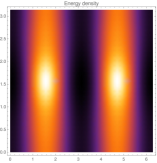
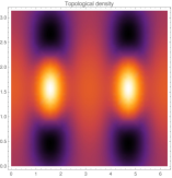
Figure 1: Energy density and topological charge density of two gauged solitons, with $n=2$, $m=0$, and $p=q=1$. Here we can see the periodic ordering of the tube-shaped configurations.

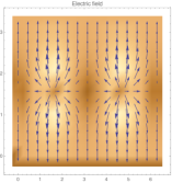
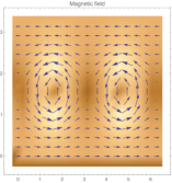
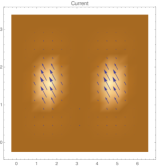
Figure 2: Electric field, magnetic field and the current of two gauged solitons, with $n=2$, $m=0$, and $p=q=1$. The electric and magnetic fields vanish in the center of the tubes while the current is completely contained inside these.

Figure 3 shows the energy density of different configurations for a given value of the topological charge ($B=5$ in this case) when the parameters $q$ and $m$ changes. For this we have imposed again the boundary conditions in Eq. (31). One can see that, as the value of $q$ increases, the peaks become more localized and their intensity also increases. On the other hand, when the value of the mass becomes larger, it is observed that the spacing between the tubes in the $r$ direction becomes irregular, in such a way that the tubes are grouped in pairs in this direction.

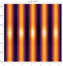
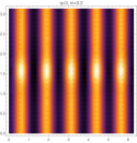
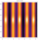
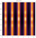
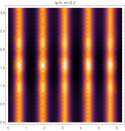
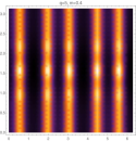
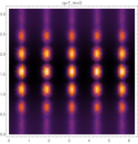
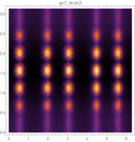
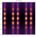
Figure 3: Comparison of the energy density for different configurations with topological charge $B=5$, as function of $q$ and $m$. Here we have considered $n=5$, $K=2$, $L=1.05$ and $p=1$.

4.2 A remark on the stability

The full stability analysis for the present gauged multi-solitonic configurations is a quite complicated task even numerically. There are two main reasons behind this fact: first of all, the field equations linearized around the gauged solitons constructed here do not reduce to a single master equation. Secondly, the problem is essentially two dimensional: namely, the linearized field equations look like a system of two-dimensional coupled Schrodinger equations which do not allow separation of variables to get effective one-dimensional problems. However, in the following subsections we will discuss the stability of these gauged solitons under two particular types of perturbations.

4.2.1 Perturbations on the profile

When the complete set of coupled field equations in a sector with non-vanishing topological charge reduce to a single equation for the profile $\alpha$ very sound arguments (see [61], [62] and references therein) suggest that a very typical unstable mode corresponds to perturbations of the profile itself which do not destroy the hedgehog property:

$$\alpha\rightarrow\alpha+\varepsilon\Psi\left(r\right)\ ,\ \ \ \varepsilon\ll 1\ .$$ (32)

One can easily see that if one linearizes Eq. (16) around a background solution $\alpha_{0}\left(r\right)$ of charge $B=np$ possesses the following zero-mode: $\Psi\left(r\right)=\partial_{r}\alpha_{0}\left(r\right)$. If one takes into account Eqs. (17) and (18), it turns out that $\Psi(r)$ has no node: therefore $\Psi(r)$ is the perturbation with the lowest energy. Obviously, this result does not imply that full stability, nevertheless it is a strong hint as often the stability of solitons with high topological charge fails precisely due to this type of perturbations.

4.2.2 Electromagnetic perturbations

Here we will shortly discuss the behavior of the above class of analytic gauged solitons under electromagnetic perturbations. As it is well known (see chapter 4 -in particular, section 4.2- of the classic reference [63]) at leading order in the ’t Hooft large N expansion, the soliton is basically unaffected in meson-soliton scattering processes (as it is quite heavy). Obviously, the same argument applies in the photon-soliton semiclassical interactions. Consequently, electromagnetic perturbations perceive the gauged solitons as an effective medium while the perturbations of the solitons are suppressed by powers of 1/N. In other words, it makes sense to only consider the reaction of the Maxwell equations to perturbations around the gauged solitons. So, let’s consider the following electromagnetic perturbation

$$A_{\mu}^{(0)}\rightarrow A_{\mu}^{(0)}+\varepsilon\bar{A}_{\mu}\ ,\ \ \ 0<\varepsilon\ll 1\ ,$$

When one considers general electromagnetic perturbations the contribution at first order in $\varepsilon$ to the current has the following form

$$J_{\mu}^{\text{pert}} =\delta_{\varepsilon}\left\{\frac{K}{2}\text{Tr}\left[\widehat{O}L_{\mu}\right]\right\}=\bar{C}_{\mu}^{\nu}\bar{A}_{\nu}\ ,$$

$$\bar{C}_{\mu}^{\nu} =-4K\sin^{2}(\alpha)\sin^{2}(q\theta)\delta_{\mu}^{\nu}\ ,$$

where $\bar{C}_{\mu}^{\nu}$ can be seen as an effective mass-like tensor. Therefore, the Maxwell equations linearized around the gauged solitons constructed in the previous sections read

$$\nabla^{\mu}f_{\mu\nu}=\bar{C}_{\mu}^{\nu}\bar{A}_{\nu}\ ,\ \ f_{\mu\nu}=\partial_{\mu}\bar{A}_{\nu}-\partial_{\nu}\bar{A}_{\mu}\ .\$$ (33)

In conclusion, the electromagnetic perturbations of the above family of gauged solitons perceive the background solutions as an effective medium whose properties are encoded in the mass-like tensor $\bar{C}_{\mu}^{\nu}$ which explicitly depends on the soliton profile $\alpha$ defined in Eqs. (16), (17) and (18).

We hope to come back on the analysis of electromagnetic response functions of this “effective medium” in a future publication.

5 Conclusions and perspectives

The first analytic examples of gauged solitons with non-vanishing topological charge and with manifest ordered structures in the gauged non-linear sigma model in (3+1)-dimensions have been constructed. The complete set of seven coupled non-linear field equations can be reduced (using a judiciously chosen ansatz) in a self-consistent way to one linear Schrodinger-like equation with an effective two dimensional periodic potential keeping alive, at the same time, the baryonic charge. The energy density, the topological charge density and the current density are periodic and the positions of their peaks manifest a crystalline order. These configurations describe gauged tubes in which (most of) the topological charge and total energy are concentrated within three-dimensional tube-shaped regions whose positions are regular in space. The electric and magnetic fields vanish at the center of the tubes and take their maximum values on their surfaces while the electromagnetic current is contained within these tube-shaped regions. Electromagnetic perturbations of these gauged tubes perceive them as an effective periodic medium whose properties can be studied explicitly in term of the solitons profile. The plots presented here are similar to the ones obtained numerically (see [23], [24], [25], [26] and references therein) in the description of nuclear spaghetti. On the other hand, in the present case the gauged solitons (besides to be analytic) also include the effects of their own electromagnetic field in a self-consistent way. These results open many interesting possibilities. One can, for instance, analyze the electromagnetic response functions of these gauged solitons in the approximation in which they are perceived as an effective medium by electromagnetic perturbations. It is also very interesting to analyze the semi-classical quantization of these gauged tubes following the classic references [7], [8], [9], [10] (however some of the techniques in the above references cannot be applied directly here since the present gauged solitons are not static, although the corresponding energy-momentum tensor is). We hope to come back on these very nice topics in future publications.

Acknowledgements

This work has been funded by Fondecyt grant 1160137. A.V. appreciates the support of CONICYT Fellowship 21151067. This work is partially supported by the National Research Foundation of Korea funded by the Ministry of Education (Grant 2018-R1D1A1B0-7048945). The Centro de Estudios Científicos (CECs) is funded by the Chilean Government through the Centers of Excellence Base Financing Program of Conicyt.

Appendix: Obtaining the field equations

Explicitly, the $SU(2)$ scalar field, according to our ansatz defined in Eqs. (12), (13), (14) and (15), is given by

$$U=\begin{pmatrix}\cos(\alpha)+i\cos(q\theta)\sin(\alpha)&ie^{-\frac{ip}{L}(t-L\phi)}\sin(q\theta)\sin(\alpha)\\ ie^{\frac{ip}{L}(t-L\phi)}\sin(q\theta)\sin(\alpha)&\cos(\alpha)-i\cos(q\theta)\sin(\alpha)\end{pmatrix}.$$

It follows that the components of $L_{\mu}=U^{-1}D_{\mu}U$ read

$$L_{t} =\frac{P}{L}\begin{pmatrix}i\sin^{2}(q\theta)\sin^{2}(\alpha)&E^{(+)}F^{(-)}\\ -E^{(-)}F^{(+)}&-i\sin^{2}(q\theta)\sin^{2}(\alpha)\end{pmatrix}\ ,\quad L_{r}=i\alpha^{\prime}\begin{pmatrix}\cos(q\theta)&E^{(+)}\sin(q\theta)\\ E^{(-)}\sin(q\theta)&-\cos(q\theta)\end{pmatrix}\ ,$$

$$L_{\theta} =q\sin(\alpha)\begin{pmatrix}-i\sin(q\theta)\cos(\alpha)&E^{(+)}G^{(+)}\\ E^{(-)}G^{(-)}&i\sin(q\theta)\cos(\alpha)\end{pmatrix}\ ,\quad L_{\phi}=P\begin{pmatrix}-i\sin^{2}(q\theta)\sin^{2}(\alpha)&-E^{(+)}F^{(-)}\\ E^{(-)}F^{(+)}&i\sin^{2}(q\theta)\sin^{2}(\alpha)\end{pmatrix}\ ,$$

where we have defined

$$P =p-2Lu\ ,\qquad F^{(\pm)}=\biggl{(}\cot(\alpha)\pm i\cos(q\theta)\biggl{)}\sin(q\theta)\sin^{2}(\alpha)\ ,$$

$$E^{(\pm)} =e^{\pm i\frac{p}{L}(L\phi-t)}\ ,\qquad G^{(\pm)}=i\cos(q\theta)\cos(\alpha)\pm\sin(\alpha)\ .$$

On the other hand, varying the Lagrangian w.r.t the $U$ field we obtain

$$\delta\mathcal{L} =\text{Tr}\biggl{[}\frac{K}{4}\delta(L^{\mu}L_{\mu})-m^{2}\delta(U+U^{-1})\biggl{]}$$

$$=\text{Tr}\biggl{[}\frac{K}{2}L^{\mu}\delta L_{\mu}-m^{2}(\delta U+\delta U^{-1})\biggl{]}\ .$$

For the non-linear sigma model term, we use

$$\delta(UU^{-1}) =0\quad\rightarrow\quad\delta U^{-1}=-U^{-1}\delta UU^{-1}\ ,$$

$$D_{\mu}(UU^{-1}) =0\quad\rightarrow\quad D_{\mu}U^{-1}=-U^{-1}D_{\mu}UU^{-1}=-L_{\mu}U^{-1}\ ,$$

so that

$$\delta L_{\mu} =\delta(U^{-1}D_{\mu}U)$$

$$=-U^{-1}\delta UU^{-1}D_{\mu}U+U^{-1}\delta D_{\mu}U$$

$$=-U^{-1}\delta UL_{\mu}+L_{\mu}U^{-1}\delta U+D_{\mu}(U^{-1}\delta U)\ .$$ (34)

From the above, the variation of the non-linear sigma model term (using the cyclicity of the trace for the first two terms) becomes

$$\text{Tr}(L^{\mu}\delta L_{\mu}) =\text{Tr}(L^{\mu}D_{\mu}(U^{-1}\delta U))$$

$$=-\text{Tr}(D_{\mu}L^{\mu}U^{-1}\delta U)+\text{Tr}(D_{\mu}(U^{-1}\delta UL^{\mu}))\ ,$$ (35)

where we have integrated by parts. Now, introducing this in the variation of the Lagrangian, we obtain

$$\delta\mathcal{L} =\text{Tr}\biggl{[}-\frac{K}{2}D_{\mu}L^{\mu}U^{-1}\delta U-m^{2}(\delta U-U^{-1}\delta UU^{-1})\biggl{]}\quad+\quad\text{Boundary term}$$

$$=-\text{Tr}\biggl{[}\frac{K}{2}D_{\mu}L^{\mu}U^{-1}\delta U+m^{2}(UU^{-1}\delta U-U^{-1}U^{-1}\delta U)\biggl{]}\quad+\quad\text{Boundary term}$$

$$=-\text{Tr}\biggl{[}\left(\frac{K}{2}D_{\mu}L^{\mu}+m^{2}(U-U^{-1})\right)U^{-1}\delta U\biggl{]}\quad+\quad\text{Boundary term}\ ,$$

and because $U\neq 0$ and the first factor in the trace is in the algebra, it is necessarily that

$$D_{\mu}L^{\mu}+\frac{2m^{2}}{K}\left(U-U^{-1}\right)=0\ .$$

Replacing the $L_{\mu}$ in the previous equation we lead to the equation in Eq. (16).

References

- [1] N. Manton and P. Sutcliffe, Topological Solitons, (Cambridge University Press, Cambridge, 2007).
- [2] A. Balachandran, G. Marmo, B. Skagerstam, A. Stern, Classical Topology and Quantum States, World Scientific (1991).
- [3] J. Gasser and H. Leutwyler, Nucl. Phys. B250, 465 (1985).
- [4] V. P. Nair, Quantum Field Theory: A Modern Perspective (Springer, New York, 2005).
- [5] T. Skyrme, Proc. R. Soc. London A 260, 127 (1961); Proc. R. Soc. London A 262, 237 (1961); Nucl. Phys. 31, 556 (1962).
- [6] G. H. Derrick, J. Math. Phys. 5, 1252 (1964).
- [7] E. Witten, Nucl. Phys. B 223 (1983), 422 Nucl. Phys. B 223, 433 (1983).
- [8] A. P. Balachandran, V. P. Nair, N. Panchapakesan, S. G. Rajeev, Phys. Rev. D 28 (1983), 2830.
- [9] A. P. Balachandran, A. Barducci, F. Lizzi, V.G.J. Rodgers, A. Stern, Phys. Rev. Lett. 52 (1984), 887; A.P. Balachandran, F. Lizzi, V.G.J. Rodgers, A. Stern, Nucl. Phys. B 256, 525-556 (1985).
- [10] G. S. Adkins, C. R. Nappi, E. Witten, Nucl. Phys. B 228 (1983), 552-566.
- [11] P. de Forcrand, Simulating QCD at finite density, PoS(LAT2009)010 [arXiv:1005.0539] [INSPIRE].
- [12] N. Brambilla et al., QCD and Strongly Coupled Gauge Theories: Challenges and Perspectives, Eur. Phys. J. C 74 (2014) 2981 [arXiv:1404.3723] [INSPIRE].
- [13] K. Takayama, M. Oka, Nucl. Phys. A 551 (1993), 637-656.
- [14] V. Schön, M. Thies, Phys. Rev. D 62 (2000) 096002.
- [15] L. Brey, H. A. Fertig, R. Cote, A. H. MacDonald, Phys. Rev. Lett. 75, 2562 (1995).
- [16] I. Klebanov, Nucl. Phys. B 262 (1985) 133.
- [17] E. Wrist, G.E. Brown, A.D. Jackson, Nucl. Phys. A 468 (1987) 450.
- [18] N. Manton, Phys Lett. B 192 (1987) 177.
- [19] A. Goldhaber, N. Manton, Phys Lett. B 198 (1987), 231.
- [20] N. Manton, P. Sutcliffe, Phys. Lett. B 342 (1995) 196.
- [21] D. Harland, N. Manton, Nucl. Phys. B 935 (2018) 210.
- [22] W. K. Baskerville, Phys. Lett. B 380 (1996) 106.
- [23] D.G. Ravenhall, C.J. Pethick, J.R.Wilson, Phys. Rev. Lett. 50, 2066 (1983).
- [24] M. Hashimoto, H. Seki, M. Yamada, Prog. Theor. Phys. 71, 320 (1984).
- [25] C.J. Horowitz, D.K. Berry, C.M. Briggs, M.E. Caplan, A. Cumming, A.S. Schneider, Phys. Rev. Lett. 114, 031102 (2015).
- [26] D.K. Berry,M.E. Caplan, C.J. Horowitz, G.Huber, A.S. Schneider, Phys. Rev. C 94, 055801 (2016).
- [27] B.J. Schroers, Phys. Lett. B 356 (1995) 291–296.
- [28] K. Arthur, D.H. Tchrakian, Phys. Lett. B 378 (1996) 187–193.
- [29] J. Gladikowski, B. M. A. G. Piette, B. J. Schroers, Phys. Rev. D 53 (1996), 844.
- [30] Y. M. Cho, K. Kimm, Phys. Rev. D 52 (1995), 7325.
- [31] Y. Brihaye, D. H. Tchrakian, Nonlinearity 11 (1998) 891.
- [32] A.Yu. Loginov, V.V. Gauzshtein, Phys. Lett. B 784 (2018) 112–117.
- [33] C. Adam, C. Naya, T. Romanczukiewicz, J. Sanchez-Guillena, A. Wereszczynski, JHEP 05 (2015) 155.
- [34] C. Adam, T. Romanczukiewicz, J. Sanchez-Guillen, A. Wereszczynski, JHEP 11 (2014) 095.
- [35] A. Alonso-Izquierdo, W. Garcıa Fuertes, J. Mateos Guilarte, JHEP 02 (2015) 139.
- [36] S. Chimento, T. Ortin, A. Ruiperez, JHEP 05 (2018) 107.
- [37] D. J. Kaup, Phys. Rev. 172, 1331 (1968).
- [38] S. L. Liebling and C. Palenzuela, Living Rev. Relativ. 15, 6 (2012).
- [39] F. Canfora, H. Maeda, Phys. Rev. D 87, 084049 (2013).
- [40] F. Canfora, Phys. Rev. D 88, (2013), 065028.
- [41] S. Chen, Y. Li, Y. Yang, Phys. Rev. D 89 (2014), 025007.
- [42] F. Canfora, F. Correa, J. Zanelli, Phys. Rev. D 90, 085002 (2014).
- [43] F. Canfora, M. Di Mauro, M. A. Kurkov, A. Naddeo, Eur. Phys. J. C75 (2015) 9, 443.
- [44] E. Ayon-Beato, F. Canfora, J. Zanelli, Phys. Lett. B 752, (2016) 201-205.
- [45] F. Canfora, G. Tallarita, Nucl. Phys. B 921 (2017) 394–410.
- [46] F. Canfora, A. Paliathanasis, T. Taves and J. Zanelli, Phys. Rev. D 95, no. 6, 065032 (2017).
- [47] A. Giacomini, M. Lagos, J. Oliva and A. Vera, Phys. Lett. B 783, 193 (2018).
- [48] M. Astorino, F. Canfora, M. Lagos and A. Vera, Phys. Rev. D 97, no. 12, 124032 (2018).
- [49] P. D. Alvarez, F. Canfora, N. Dimakis and A. Paliathanasis, Phys. Lett. B 773, (2017) 401-407.
- [50] L. Aviles, F. Canfora, N. Dimakis, D. Hidalgo, Phys. Rev. D 96 (2017), 125005.
- [51] F. Canfora, M. Lagos, S. H. Oh, J. Oliva and A. Vera, Phys. Rev. D 98, no. 8, 085003 (2018).
- [52] F. Canfora, N. Dimakis, A. Paliathanasis, Eur.Phys.J. C79 (2019) no.2, 139.
- [53] F. Canfora, Eur. Phys. J. C78, no. 11, 929 (2018).
- [54] C. G. Callan Jr. and E. Witten, Nucl. Phys. B 239 (1984) 161-176.
- [55] J.M. Gipson and H.Ch. Tze, Nucl. Phys. B 183 (1981) 524.
- [56] J. Goldstone and F. Wilczek, Phys. Rev. Lett. 47 (1981) 986.
- [57] E. D’Hoker and E. Farhi, Nucl. Phys. B241 (1984) 109.
- [58] V.A. Rubakov, Nucl. Phys. B256 (1985) 509.
- [59] B.M.A.G. Piette, D. H. Tchrakian, Phys.Rev. D 62 (2000) 025020.
- [60] E. Radu, D. H. Tchrakian, Phys. Lett. B 632 (2006) 109–113.
- [61] M. Shifman, “Advanced Topics in Quantum Field Theory: A Lecture Course” Cambridge University Press, (2012).
- [62] M. Shifman, A. Yung, “Supersymmetric Solitons” Cambridge University Press, (2009).
- [63] H. Weigel, Chiral Soliton Models for Baryons, Lecture Notes in Physics (Springer, 2008).