Data-Dependent Differentially Private Parameter Learning for Directed Graphical Models

Data-Dependent Differentially Private Parameter Learning for Directed Graphical Models – Supplementary Material

Abstract

Directed graphical models (DGMs) are a class of probabilistic models that are widely used for predictive analysis in sensitive domains such as medical diagnostics. In this paper, we present an algorithm for differentially private learning of the parameters of a DGM. Our solution optimizes for the utility of inference queries over the DGM and adds noise that is customized to the properties of the private input dataset and the graph structure of the DGM. To the best of our knowledge, this is the first explicit data-dependent privacy budget allocation algorithm in the context of DGMs. We compare our algorithm with a standard data-independent approach over a diverse suite of benchmarks and demonstrate that our solution requires a privacy budget that is roughly $3\times$ smaller to obtain the same or higher utility.

1 Introduction

Directed graphical models (DGMs) are a class of probabilistic models that are widely used in causal reasoning and predictive analytics  (PGMbook). A typical use case for these models is answering “what-if” queries over domains that often work with sensitive information. For example, DGMs are used in medical diagnosis for answering questions, such as what is the most probable disease given a set of symptoms (DGM1). In learning such models, it is common that the underlying graph structure of the model is publicly known. For instance, in the case of medical data, the dependencies between several physiological symptoms and diseases are well established, standardized, and publicly available. However, the parameters of the model have to be learned from observations. These observations may contain sensitive information as in the case of medical applications. Hence, learning and publicly releasing the parameters of the probabilistic model may lead to privacy violations (attack1; attack2), and thus, the need for privacy-preserving learning mechanisms for DGMs.

In this paper, we focus on the problem of privacy-preserving learning of the parameters of a DGM. For our privacy definition, we use differential privacy (DP) (dwork) – currently the de-facto standard for privacy. We consider the setting when the structure of the target DGM is publicly known and the parameters of the model are learned from fully observed data. In this case, all parameters can be estimated via counting queries over the input observations (also referred to as data set in the remainder of the paper). The direct way to ensure differential privacy is to add suitable noise to the observations using the standard Laplace mechanism (dwork). Unfortunately, this method is data-independent, i.e., the noise added to the base observations is oblivious of the properties of the input data set and the structure of the DGM, resulting in sub-optimal utility. To address this issue, we turn to data-dependent methods which add noise that is customized to the properties of the input data sets (DAWA; AHP; data1; hist; hist2; DPcube; Kotsogiannis:2017:PDD:3035918.3035945).

We propose a data-dependent, $\epsilon$-DP algorithm for learning the parameters of a DGM over fully observed data. Our goal is to minimize errors in arbitrary inference queries that are subsequently answered over the learned DGM. The main contributions are:

(1) Explicit data-dependent privacy-budget allocation: Our algorithm computes the parameters of the conditional probability distribution of each random variable in the DGM via separate measurements from the input data set. This lets us optimize the privacy budget allocation across the different variables with the objective of reducing the error in inference queries. We formulate this optimization objective in a data-dependent manner – our optimization objective is informed by both the private input data set and the public graph structure of the DGM. To the best of our knowledge, this is the first work to propose explicit data-dependent privacy-budget allocation in the context of DGMs. We evaluate our algorithm on four DGM benchmarks and demonstrate that our scheme only requires a privacy budget of $\epsilon=1.0$ to yield the same utility that a data-independent baseline achieves with a much higher $\epsilon=3.0$. Specifically, our baseline is based on (Bayes4) which is the most recent work that explicitly deals with differentially private parameter estimation for DGMs.

(2) New theoretical results: To preserve privacy, we add noise to the parameters of the DGM. To understand how this noise propagates to inference queries, we provide two new theoretical results on the upper and lower bound of the error of inference queries. The upper bound has an exponential dependency on the treewidth of the DGM while the lower bound depends on its maximum degree. We also provide a formulation to compute the sensitivity (sensitivity1) of the parameters associated with a node of a DGM targeting the probability distribution of its child nodes only. To the best of our knowledge, these theoretical results are novel.

2 Background

In this section, we review basic background material relevant to this paper.

Directed Graphical Models: A directed graphical model (DGM) or a Bayesian network is a probabilistic model that is represented as a directed acyclic graph, $\mathcal{G}$ .

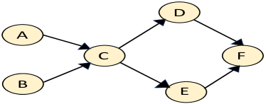
Figure 1: An example directed graphical model

The nodes of the graph represent random variables and the edges encode conditional dependencies between the variables. The graphical structure of the DGM represents a factorization of the joint probability distribution of these random variables. Specifically, given a DGM with graph $\mathcal{G}$ , let $X_{1},\ldots,X_{n}$ be the random variables corresponding to the nodes of $\mathcal{G}$ and $X_{pa_{i}}$ denote the set of parents in $\mathcal{G}$ for the node corresponding to variable $X_{i}$ . The joint probability distribution factorizes as

where each factor $P[X_{i}|X_{pa_{i}}]$ corresponds to a conditional probability distribution (CPD). For example, for the DGM depicted by Fig. 1, we have $P[A,B,C,D,E,F]=P[A]\cdot P[B]\cdot P[C|A,B]\cdot P[D|C]\cdot P[E|C]\cdot$ $P[F|D,E]$. For DGMs with discrete random variables, each CPD can be represented as a table of parameters $\Theta_{x_{i}|x_{pa_{i}}}$ where each parameter corresponds to a conditional probability and $x_{i}$ and $x_{pa_{i}}$ denote variable assignments $X_{i}=x_{i}$ and $X_{pa_{i}}=x_{pa_{i}}$ .

A key task in DGMs is parameter learning. Given a DGM with a graph structure $\mathcal{G}$ , the goal of parameter learning is to estimate each $\Theta_{x_{i}|x_{pa_{i}}},$ a task solved via maximum likelihood estimation (MLE). In the presence of fully observed data $\mathcal{D}$ (i.e., data corresponding to all the nodes of $\mathcal{G}$ is available), the maximum likelihood estimates of the CPD parameters take the closed-form (PGMbook)

$$\small\Theta_{x_{i}|x_{pa_{i}}}=C[x_{i},x_{pa_{i}}]/C[x_{pa_{i}}]$$ (2)

where $C[x_{i}]$ is the number of records in $\mathcal{D}$ with $X_{i}=x_{i}$ .

After learning, the DGM is used to answer inference queries, i.e., queries that compute the probabilities of certain events (variables) of interest. Inference queries can also include evidence (a subset of the nodes has a fixed assignment). There are three types inference queries in general:

(1) Marginal inference: This is used to answer queries of the type "what is the probability of a given variable if all others are marginalized". An example marginal inference query for the DGM in Fig. 1 is $P[F=0]=\sum_{A}\sum_{B}\sum_{C}\sum_{D}\sum_{F}P[A,B,C,D,E,F=0]$ .

(2) Conditional Inference: This type of query answers the probability distribution of some variable conditioned on some evidence $e$. An example conditional inference query for the DGM in Fig. 1 is $P[A|F=0]=$ $\frac{P[A,F=0]}{P[F=0]}$.

(3) Maximum a posteriori (MAP) inference: This type of query asks for the most likely assignment of variables. An example MAP query for the DGM in Fig. 1 is $\max_{A,B,C,D,E}\{P[A,B,C,D,E,F=0]\}$ .

For DGMs, inference queries can be answered exactly by the variable elimination (VE) algorithm (PGMbook) which is described in detail in Appx. LABEL:app:DGM. The basic idea is that we "eliminate" one variable at a time following a predefined order $\prec$ over the graph nodes. Let $\Phi$ denote a set of probability factors $\phi$ (initialized with all the CPDs of the DGM) and $Z$ denote the variable to be eliminated. First, all probability factors involving $Z$ are removed from $\Phi$ and multiplied together to generate a new product factor. Next, $Z$ is summed out from this combined factor, generating a new factor $\boldsymbol{\phi}$ that is entered into $\Phi$ . Thus, VE corresponds to repeated sum-product computations: $\boldsymbol{\phi}=\sum_{Z}\prod_{\phi\in\Phi}\phi$ .

Additionally, we define a term Markov blanket which is used in Sec. LABEL:sec:Alg:desc.

Definition 2.1 (Markov Blanket).

The Markov blanket, denoted by $\mathpzc{P}(X)$ , for a node $X$ in a graphical model is the set of all nodes such that given $\mathpzc{P}(X)$ , $X$ is conditionally independent of all the other nodes. (markovblanket).

In a DGM, the Markov blanket of a node consists of its child nodes, parent nodes, and the parents of its child nodes. For example, in Fig. 1, $\mathcal{P}(D)=\{C,E,F\}$.

Differential Privacy: We formally define differential privacy (DP) as follows:

Definition 2.2 (Differential Privacy).

A randomized algorithm $\mathcal{A}$ satisfies $\epsilon$-differential privacy ($\epsilon$-DP), where $\epsilon>0$ is a privacy parameter, iff for any two data sets $\mathcal{D}$ and $\mathcal{D}^{\prime}$ that differ in a single record, we have

$$\small\forall t\in Range(\mathcal{A}),P\big{[}\mathcal{A}(\mathcal{D})=t\big{]}\leq e^{\epsilon}P\big{[}\mathcal{A}(\mathcal{D}^{\prime})=t\big{]}$$ (3)

In our setting, $\mathcal{A}$ (in Eq. (3)) corresponds to an algorithm for learning the parameters of a DGM with a publicly known graph structure from a fully observed data set $\mathcal{D}$.

When applied multiple times, the DP guarantee degrades gracefully as follows.

Theorem 2.1 (Sequential Composition).

If $\mathcal{A}_{1}$ and $\mathcal{A}_{2}$ are $\epsilon_{1}$-DP and $\epsilon_{2}$-DP algorithms that use independent randomness, then releasing the outputs $(\mathcal{A}_{1}(\mathcal{D}),\mathcal{A}_{2}(\mathcal{D}))$ on database $\mathcal{D}$ satisfies $(\epsilon_{1}+\epsilon_{2})$-DP.

Any post-processing computation performed on the noisy output of a DP algorithm does not degrade privacy.

Theorem 2.2 (Post-processing).

Let $\mathcal{A}:\mathcal{D}\mapsto R$ be a $\epsilon$-DP algorithm. Let $f:R\mapsto R^{\prime}$ be an arbitrary randomized mapping. Then $f\circ\mathcal{A}:\mathcal{D}\mapsto R^{\prime}$ is $\epsilon$-DP.

The privacy guarantee of a DP algorithm can be amplified by a preceding sampling step (PAClearning; Amplification). Let $\mathcal{A}$ be an $\epsilon$-DP algorithm and $\mathcal{D}$ be a data set. Let $\mathcal{A}^{\prime}$ be an algorithm that runs $\mathcal{A}$ on a random subset of $\mathcal{D}$ obtained by sampling it with probability $\beta$ .

Lemma 2.3 (Privacy Amplification).

Algorithm $\mathcal{A}^{\prime}$ will satisfy $\epsilon^{\prime}$-DP where $\epsilon^{\prime}=ln(1+\beta(e^{\epsilon}-1))$

The Laplace mechanism is a standard algorithm to achieve differential privacy (dwork). In this mechanism, in order to output $f(\mathcal{D})$ where $f:\mathcal{D}\mapsto R$ , an $\epsilon$-DP algorithm $\mathcal{A}$ publishes $f(\mathcal{D})+Lap\Big{(}\frac{\Delta f}{\epsilon}\Big{)}$ where $\Delta f=\max_{\mathcal{D},\mathcal{D}^{\prime}}||f(\mathcal{D})-f(\mathcal{D}^{\prime})||_{1}$ is known as the sensitivity of the function. The probability density function of $Lap(b)$ is given by $\mathbf{f}(x)={\frac{1}{2b}}e^{\left(-{\frac{|x-\mu|}{b}}\right)}$ . The sensitivity of the function $f$ is the maximum magnitude by which an individual’s data can change $f$ . The sensitivity of counting queries is 1.

Next, we define two terms, namely marginal table and mutually consistent marginal tables, that are used in Sec. LABEL:sec:Alg:desc.

Let $\mathcal{D}$ be a data set defined over attributes $\mathcal{X}$ and $\mathbf{X}$ be an attribute set such that $\mathbf{X}=\{X_{1},\cdots,X_{k}\},\mathbf{X}\subseteq\mathcal{X}$ . Let $s=\prod_{i=1}^{k}|dom(X_{i})|$ and $dom(\mathbf{X)}=\{v_{1},\cdots,v_{s}\}$ represent the domain of $\mathbf{X}$ . The marginal table for the attribute set $\mathbf{X}$ denoted by $M_{\mathbf{X}}$ , is computed as follows:

(1) Populate the entries of table $T_{\mathbf{X}}$ of size $s$ from $\mathcal{D}$ such that each entry $j\in[s],T_{\mathbf{X}}[j]=\#$ records in $\mathcal{D}$ with $\mathbf{X}=v_{j}$ . This step is also called materialization.

(2) Compute $M_{\mathbf{X}}$ from $T_{\mathbf{X}}$ such that $M_{\mathbf{X}}[j]=T_{\mathbf{X}}[j]/\sum_{i=1}^{s}T_{\mathbf{X}}[i],j\in[s]$ .

Thus the entries of $M_{\mathbf{X}}$ corresponds to the values of the joint probability distribution over the attributes in $\mathbf{X}$ .

Let $Attr(M)$ denote the set of attributes on which a marginal table $M$ is defined and $M_{1}\equiv M_{2}$ denote that the two marginal tables have the same values for every entry.

Definition 2.3 (Mutually Consistent Marginal Tables).

Two noisy marginal tables $\tilde{M}_{i}$ and $\tilde{M}_{j}$ are defined to be mutually consistent iff the marginal table over the attributes in $Attr(\tilde{M}_{i})\cap Attr(\tilde{M}_{j})$ reconstructed from $\tilde{M}_{i}$ is exactly the same as the one reconstructed from $\tilde{M}_{j}$ , i.e.,

$$\tilde{M}_{i}[Attr(\tilde{M}_{i})\cap Attr(\tilde{M}_{j})]\equiv\tilde{M}_{j}[Attr(\tilde{M}_{i})\cap Attr(\tilde{M}_{j})]$$ (4)

3 Data-Dependent Differentially Private Parameter Learning for DGMs

In this section, we describe our proposed solution for differentially private learning of the parameters of a fully observed DGM by adding data and structure dependent noise.

3.1 Problem Setting

Let $\mathcal{D}$ be a sensitive data set of size $m$ with attributes $\mathcal{X}=\langle X_{1},\cdots,X_{n}\rangle$ and let $\mathcal{N}=\langle\mathcal{G},\Theta\rangle$ be the DGM of interest. The graph structure $\mathcal{G}$ of $\mathcal{N}$ defined over the attribute set $\mathcal{X}$ is publicly known. Our goal is to learn the parameters $\Theta$ , i.e., the CPDs of $\mathcal{N}$ , in a data-dependent differentially private manner from $\mathcal{D}$ such that the error in inference queries over the $\epsilon$-DP DGM is minimized.

3.2 Key Ideas

Our solution is based on the following two key observations:

(1) The parameters $\Theta[X_{i}|X_{{pa}_{i}}]$ of the DGM $\mathcal{N}$ can be estimated separately via counting queries over the empirical marginal table of the attribute set $X_{i}\cup X_{pa_{i}}$ .

(2) The factorization over $\mathcal{N}$ decomposes the overall $\epsilon$-DP learning problem into a set of separate $\epsilon$-DP learning sub-problems (one for each CPD). For example, for the DGM in Fig. 1, the following six CPDs have to be learned separately $\{P[A],P[B],P[C|A,B],P[D|C],P[E|C],$ $P[F|D,E]\}$ . Thus the total privacy budget has to be divided among these sub-problems. However, due to the structure of the graph and the data set, some nodes will have more impact on inference queries than others. Hence, allocating more budget (and thus, getting better accuracy) to these nodes will result in reduced overall error for the inference queries.

Our method is outlined in Alg. 1 and proceeds in two stages. In the first stage, we obtain preliminary noisy measurements of the parameters of $\mathcal{N}$ which are used along with some graph specific properties (the height and out-degree of each node) to formulate a data-dependent optimization objective for privacy budget allocation. The solution of this objective is then used in the second stage to compute the final parameters. For instance, for the DGM in Fig. 1, node $A$ (root node) would typically have a higher privacy budget than node $F$ (leaf node). In summary, if $\epsilon^{B}$ is the total privacy budget available, we spend $\epsilon^{I}$ to obtain preliminary parameter measurements in Stage I and the remaining $\epsilon^{B}-\epsilon^{I}$ is used for the final parameter computation in Stage II, after optimal allocation across the marginal tables. As a result, our scheme only requires a privacy budget of $\epsilon=1.0$ to yield the same utility that a standard data-independent method achieves with $\epsilon=3.0$ (Sec. LABEL:sec:evaluation).

Next, we describe our algorithm in detail and highlight how we address the two core technical challenges in our solution:

(1) how to reduce the privacy budget cost for the first stage $\epsilon^{I}$ (equivalently increase $\epsilon^{B}$-$\epsilon^{I}$) (Alg. 1, Lines 1-3), and

(2) what properties of the data set and the graph should the optimization objective be based on (Alg. 1, Lines 5-11).

Algorithm 1 Differentially private learning of the parameters of a directed graphical model

Input:$\mathcal{D}$- Input data set of size $m$with attributes                

$\mathcal{X}=\langle X_{1},\cdots,X_{n}\rangle$

;           $\mathcal{G}$- Graph Structure of DGM $\mathcal{N}$;           $\epsilon^{B}$- Total privacy budget;           $\beta$- Sampling rate for Stage I;          $\epsilon^{I}$- Privacy budget for Stage I Output:$\widetilde{\Theta}$- Noisy parameters of $\mathcal{N}$Stage I:Optimization objective formulation for privacy            budget allocation $\epsilon=\ln\big(\frac{e^{\epsilon^{I}}-1}{\beta}+1\big{missing})$$\rhd$Computing privacy parameter Construct a new dataset $\mathcal{D}^{\prime}$by sampling $\mathcal{D}$with probability $\beta$$\mathpzc{E}=[\frac{\epsilon}{n},\cdots,\frac{\epsilon}{n}]$

$\widehat{\Theta},\widehat{T},\widehat{T}_{pa}=$

$ComputeParameters$

$(\mathcal{D}^{\prime},\mathpzc{E})$

for$i=1$to $n$$\widetilde{{\delta}_{i}}$=

$ComputeError$

$(i,\widehat{T}_{i},\widehat{T}_{pa_{i}})$

$\rhd$Estimating error of parameters for $X_{i}$using Eq. ()      $h_{i}$= Height of node $X_{i}$$o_{i}$= Out-degree of node $X_{i}$

$\widetilde{\Delta}^{\mathcal{N}}_{i}$

=

$ComputeSensitivity$

$(i,\widehat{\Theta})$

$\rhd$Computing sensitivity of the parameters using Eq. ()      

$W[i]=(h_{i}+1)\cdot(o_{i}+1)\cdot(\widetilde{\Delta}^{\mathcal{N}}_{i}+1)$

end for

$\mathcal{F}_{\mathcal{G},\mathcal{D}}=\sum_{i=1}^{n-1}W[i]\cdot\widetilde{\delta_{i}}/{\epsilon_{i}}+W[n]\cdot\widetilde{\delta_{n}}/(\epsilon^{B}-\epsilon^{I}-\sum_{i=1}^{n-1}\epsilon_{i})$

$\rhd$Optimization Objective