The Label Complexity of Active Learning from Observational Data

Abstract

Counterfactual learning from observational data involves learning a classifier on an entire population based on data that is observed conditioned on a selection policy. This work considers this problem in an active setting, where the learner additionally has access to unlabeled examples and can choose to get a subset of these labeled by an oracle.

Prior work on this problem uses disagreement-based active learning, along with an importance weighted loss estimator to account for counterfactuals, which leads to a high label complexity. We show how to instead incorporate a more efficient counterfactual risk minimizer into the active learning algorithm. This requires us to modify both the counterfactual risk to make it amenable to active learning, as well as the active learning process to make it amenable to the risk. We provably demonstrate that the result of this is an algorithm which is statistically consistent as well as more label-efficient than prior work.

1 Introduction

Counterfactual learning from observational data is an emerging problem that arises naturally in many applications. In this problem, the learner is given observational data – a set of examples selected according to some policy along with their labels – as well as access to the policy that selects the examples, and the goal is to construct a classifier with high performance on an entire population, not just the observational data distribution. An example is learning to predict if a treatment will be effective based on features of a patient. Here, we have some observational data on how the treatment works for patients that were assigned to it, but if the treatment is given only to a certain category of patients, then the data is not reflective of the population. Thus the main challenge in counterfactual learning is how to counteract the effect of the observation policy and build a classifier that applies more widely.

This work considers counterfactual learning in the active setting, which has received very recent attention in a few different contexts [25, 21, 3]. In addition to observational data, the learner has an online stream of unlabeled examples drawn from the underlying population distribution, and the ability to selectively label a subset of these in an interactive manner. The learner’s goal is to again build a classifier while using as few label queries as possible. The advantage of the active over the passive is its potential for more label-efficient solutions; the question however is how to do this algorithmically.

Prior work in this problem has looked at both probabilistic inference [21, 3] as well as a standard classification [25], which is the setting of our work. [25] uses a modified version of disagreement-based active learning [7, 9, 4, 11], along with an importance weighted empirical risk to account for the population. However, a problem with this approach is that the importance weighted risk estimator can have extremely high variance when the importance weights – that reflect the inverse of how frequently an instance in the population is selected by the policy – are high; this may happen if, for example, certain patients are rarely given the treatment. This high variance in turn results in high label requirement for the learner.

The problem of high variance in the loss estimator is addressed in the passive case by minimizing a form of counterfactual risk [22] – an importance weighted loss that combines a variance regularizer and importance weight clipping or truncation to achieve low generalization error. A plausible solution is to use this risk for active learning as well. However, this cannot be readily achieved for two reasons. The first is that the variance regularizer itself is a function of the entire dataset, and is therefore challenging to use in interactive learning where data arrives sequentially. The second reason is that the minimizer of the (expected) counterfactual risk depends on $n$, the data size, which again is inconvenient for learning in an interactive manner.

In this work, we address both challenges. To address the first, we use, instead of a variance regularizer, a novel regularizer based on the second moment; the advantage is that it decomposes across multiple segments of the data set as which makes it amenable for active learning. We provide generalization bounds for this modified counterfactual risk minimizer, and show that it has almost the same performance as counterfactual risk minimization with a variance regularizer [22]. The second challenge arises because disagreement-based active learning ensures statistical consistency by maintaining a set of plausible minimizers of the expected risk. This is problematic when the minimizer of the expected risk itself changes between iterations as in the case with our modified regularizer. We address this challenge by introducing a novel variant of disagreement-based active learning which is always guaranteed to maintain the population error minimizer in its plausible set.

Additionally, to improve sample efficiency, we then propose a third novel component – a new sampling algorithm for correcting sample selection bias that selectively queries labels of those examples which are underrepresented in the observational data. Combining these three components gives us a new algorithm. We prove this newly proposed algorithm is statistically consistent – in the sense that it converges to the true minimizer of the population risk given enough data. We also analyze its label complexity, show it is better than prior work [25], and demonstrate the contribution of each component of the algorithm to the label complexity bound.

2 Related Work

We consider learning with logged observational data where the logging policy that selects the samples to be observed is known to the learner. The standard approach is importance sampling to derive an unbiased loss estimator [19], but this is known to suffer from high variance. One common approach for reducing variance is to clip or truncate the importance weights [6, 22], and we provide a new principled method for choosing the clipping threshold with theoretical guarantees. Another approach is to add a regularizer based on empirical variance to the loss function to favor models with low loss variance [17, 22, 18]. Our second moment regularizer achieves a similar effect, but has the advantage of being applicable to active learning with theoretical guarantees.

In this work, in addition to logged observational data, we allow the learner to actively acquire additional labeled examples. The closest to our work is [25], the only known work in the same setting. [25] and our work both use disagreement-based active learning (DBAL) framework [7, 9, 4, 11] and multiple importance sampling [24] for combining actively acquired examples with logged observational data. [25] uses an importance weighted loss estimator which leads to high variance and hence high sample complexity. In our work, we incorporate a more efficient variance-controlled importance sampling into active learning and show that it leads to a better label complexity.

[3] and [21] consider active learning for predicting individual treatment effect which is similar to our task. They take a Bayesian approach which does not need to know the logging policy, but assumes the true model is from a known distribution family. Additionally, they do not provide label complexity bounds. A related line of research considers active learning for domain adaptation, and their methods are mostly based on heuristics [20, 27], utilizing a clustering structure [14], or non-parametric methods [15]. In other related settings, [26] considers warm-starting contextual bandits targeting at minimizing the cumulative regret instead of the final prediction error; [16] studies active learning with bandit feedback without any logged observational data.

3 Problem Setup

We are given an instance space $\mathcal{X}$, a label space $\mathcal{Y}=\{-1,+1\}$, and a hypothesis class $\mathcal{H}\subset\mathcal{Y}^{\mathcal{X}}$. Let $D$ be an underlying data distribution over $\mathcal{X}\times\mathcal{Y}$. For simplicity, we assume $\mathcal{H}$ is a finite set, but our results can be generalized to VC-classes by standard arguments [23, 18].

In the passive setting for learning with observational data, the learner has access to a logged observational dataset generated from the following process. First, $m$ examples $\{(X_{t},Y_{t})\}_{t=1}^{m}$ are drawn i.i.d. from $D$. Then a logging policy $Q_{0}:\mathcal{X}\rightarrow[0,1]$ that describes the probability of observing the label is applied. In particular, for each example $(X_{t},Y_{t})$ ($1\leq t\leq m$), an independent Bernoulli random variable $Z_{t}$ with expectation $Q_{0}(X_{t})$ is drawn, and then the label $Y_{t}$ is revealed to the learner if $Z_{t}=1$. We call $T_{0}=\{(X_{t},Y_{t},Z_{t})\}_{t=1}^{m}$ the logged dataset. We assume the learner knows the logging policy $Q_{0}$, and only observes instances $\{X_{t}\}_{t=1}^{m}$, indicators $\{Z_{t}\}_{t=1}^{m}$, and revealed labels $\{Y_{t}\mid Z_{t}=1\}_{t=1}^{m}$.

In the active learning setting, in addition to the logged dataset, the learner has access to a stream of online data. In particular, there is a stream of additional $n$ examples $\{(X_{t},Y_{t})\}_{t=m+1}^{m+n}$ drawn i.i.d. from distribution $D$. At time $t$ ($m<t\leq m+n$), the learner applies a query policy to compute an indicator $Z_{t}\in\{0,1\}$, and then the label $Y_{t}$ is revealed if $Z_{t}=1$. The computation of $Z_{t}$ may in general be randomized, and is based on the observed logged data $T_{0}$, previously observed instances $\{X_{i}\}_{i=m+1}^{t}$, decisions$\{Z_{i}\}_{i=m+1}^{t-1}$, and observed labels $\{Y_{i}\mid Z_{i}=1\}_{i=m+1}^{t-1}$.

We focus on the active learning setting, and the goal of the learner is to learn a classifier $h\in\mathcal{H}$ from observed logged data and online data. Fixing $D$, $Q_{0}$, $m$, $n$, the performance is measured by: (1) the error rate $l(h):=\Pr_{D}(h(X)\neq Y)$ of the output classifier, and (2) the number of label queries on the online data. Note that the error rate is over the entire population $D$ instead of conditioned on the logging policy, and that we assume the labels of the logged data $T_{0}$ come at no cost. In this work, we are interested in the situation where $n$, the size of the online stream, is smaller than $m$.

Notation

Unless otherwise specified, all probabilities and expectations are over the draw of all random variables $\{(X_{t},Y_{t},Z_{t})\}_{t=1}^{m+n}$. Define $q_{0}=\inf_{x}Q_{0}(x)$. Define the optimal classifier $h^{\star}=\arg\min_{h\in\mathcal{H}}l(h)$, $\nu=l(h^{\star})$. For any $r>0,h\in\mathcal{H}$, define the $r-$ball around $h$ as $B(h,r)=\left\{h^{\prime}\in\mathcal{H}:\Pr(h(X)\neq h^{\prime}(X))\leq r\right\}$. For any $C\subseteq\mathcal{H}$, define the disagreement region $\text{DIS}(C)=\{x\in\mathcal{X}:\exists h_{1}\neq h_{2}\in C,h_{1}(X)\neq h_{2}(X)\}$.

Due to space limit, all proofs are postponed to Appendix.

4 Variance-Controlled Importance Sampling for Passive Learning with Observational Data

In the passive setting, the standard method to overcome sample selection bias is to optimize the importance weighted (IW) loss $l(h,T_{0})=\frac{1}{m}\sum_{t}\frac{\mathds{1}\{h(X_{t})\neq Y_{t}\}Z_{t}}{Q_{0}(X_{t})}$. This loss is an unbiased estimator of the population error $\Pr(h(X)\neq Y)$, but its variance $\frac{1}{m}\mathbb{E}(\frac{\mathds{1}\{h(X)\neq Y\}Z}{Q_{0}(X)}-l(h))^{2}$ can be high, leading to poor solutions. Previous work addresses this issue by adding a variance regularizer [17, 22, 18] and clipping/truncating the importance weight [6, 22]. However, the variance regularizer is challenging to use in interactive learning when data arrives sequentially, and it is unclear how the clipping/truncating threshold should be chosen to yield good theoretical guarantees.

In this paper, as an alternative to the variance regularizer, we propose a novel second moment regularizer which achieves a similar error bound to the variance regularizer [18]; and this motivates a principled choice of the clipping threshold.

4.1 Second-Moment-Regularized Empirical Risk Minimization

Intuitively, between two classifiers with similarly small training loss $l(h,T_{0})$, the one with lower variance should be preferred, since its population error $l(h)$ would be small with a higher probability than the one with higher variance. Existing work encourages low variance by regularizing the loss with the estimated variance $\hat{\text{Var}}(h,T_{0})=\frac{1}{m}\sum_{i}(\frac{\mathds{1}\{h(X_{i})\neq Y_{i}\}Z_{i}}{Q_{0}(X_{i})})^{2}-l(h,T_{0})^{2}$. Here, we propose to regularize with the estimated second moment $\hat{\text{V}}(h,T_{0})=\frac{1}{m}\sum_{i}(\frac{\mathds{1}\{h(X_{i})\neq Y_{i}\}Z_{i}}{Q_{0}(X_{i})})^{2}$, an upper bound of $\hat{\text{Var}}(h,T_{0})$. We have the following generalization error bound for regularized ERM.

Theorem 1.

Let $\hat{h}=\arg\min_{h\in\mathcal{H}}l(h,T_{0})+\sqrt{\frac{4\log\frac{|\mathcal{H}|}{\delta}}{m}\hat{\text{V}}(h,T_{0})}$. For any $\delta>0$, then with probability at least $1-\delta$, $l(\hat{h})-l(h^{\star})\leq\frac{28\log\frac{|\mathcal{H}|}{\delta}}{3mq_{0}}+\sqrt{\frac{4\log\frac{|\mathcal{H}|}{\delta}}{m}\mathbb{E}\frac{\mathds{1}\{h^{\star}(X)\neq Y\}}{Q_{0}(X)}}+\frac{\sqrt{4\log\frac{|\mathcal{H}|}{\delta}}}{m^{\frac{3}{2}}q_{0}^{2}}.$

Theorem 1 shows an error rate similar to the one for the variance regularizer [18]. However, the advantage of using the second moment is the decomposability: $\hat{\text{V}}(h,S_{1}\cup S_{2})=\frac{|S_{1}|}{|S_{1}|+|S_{2}|}\hat{\text{V}}(h,S_{1})+\frac{|S_{2}|}{|S_{1}|+|S_{2}|}\hat{\text{V}}(h,S_{2})$. This makes it easier to analyze for active learning that we will discuss later.

Recall for the unregularized importance sampling loss minimizer $\hat{h}_{\text{IW}}=\arg\min_{h\in\mathcal{H}}l(h,T_{0})$, the error bound is $\tilde{O}(\frac{\log|\mathcal{H}|}{mq_{0}}+\sqrt{\frac{\log|\mathcal{H}|}{m}\min(\frac{l(h^{\star})}{q_{0}},\mathbb{E}\frac{1}{Q_{0}(X)})})$ [8, 25]. In Theorem 1, the extra $\frac{1}{m^{\frac{3}{2}}q_{0}^{2}}$ term is due to the deviation of $\sqrt{\hat{\text{V}}(h,T_{0})}$ around $\sqrt{\mathbb{E}\frac{\mathds{1}\{h(X)\neq Y\}}{Q_{0}(X)}}$, and is negligible when $m$ is large. In this case, learning with a second moment regularizer gives a better generalization bound.

This improvement in generalization error is due to the regularizer instead of tighter analysis. Similar to [17, 18], we show in Theorem 2 that for some distributions, the error bound in Theorem 1 cannot be achieved by any algorithm that simply optimizes the unregularized empirical loss.

Theorem 2.

For any $0<\nu<\frac{1}{3}$, $m\geq\frac{49}{\nu^{2}}$, there is a sample space $\mathcal{X}\times\mathcal{Y}$, a hypothesis class $\mathcal{H}$, a distribution $D$, and a logging policy $Q_{0}$ such that $\frac{\nu}{q_{0}}>\mathbb{E}\frac{\mathds{1}\{h^{\star}(X)\neq Y\}}{Q_{0}(X)}$, and that with probability at least $\frac{1}{100}$ over the draw of $S=\{(X_{t},Y_{t},Z_{t})\}_{t=1}^{m}$, if $\hat{h}=\arg\min_{h\in\mathcal{H}}l(h,S)$, then $l(\hat{h})\geq l(h^{\star})+\frac{1}{mq_{0}}+\sqrt{\frac{\nu}{mq_{0}}}$.

4.2 Clipped Importance Sampling

The variance and hence the error bound for second-moment regularized ERM can still be high if $\frac{1}{Q_{0}(x)}$ is large. This $\frac{1}{Q_{0}(X)}$ factor arises inevitably to guarantee the importance weighted estimator is unbiased. Existing work alleviates the variance issue at the cost of some bias by clipping or truncating the importance weight. In this paper, we focus on clipping, where the loss estimator becomes $l(h;T_{0},M):=\frac{1}{m}\sum_{i=1}^{m}\frac{\mathds{1}\{h(X_{i})\neq Y_{i}\}Z_{i}}{Q_{0}(X_{i})}\mathds{1}[\frac{1}{Q_{0}(X_{i})}\leq M]$. This estimator is no longer unbiased, but as the weight is clipped at $M$, so is the variance. Although studied previously [6, 22], to the best of our knowledge, it remains unclear how the clipping threshold $M$ can be chosen in a principled way.

We propose to choose $M_{0}=\inf\{M^{\prime}\geq 1\mid\frac{2M^{\prime}\log\frac{|\mathcal{H}|}{\delta}}{m}\geq\Pr_{X}(\frac{1}{Q_{0}(X)}>M^{\prime})\}$. This choice minimizes an error bound for the clipped second-moment regularized ERM and we formally show this in Appendix E. Example 30 in Appendix E shows this clipping threshold avoids outputting suboptimal classifiers. The choice of $M_{0}$ implies that the clipping threshold should be larger as the sample size $m$ increases, which confirms the intuition that with a larger sample size the variance becomes less of an issue than the bias. We have the following generalization error bound.

Theorem 3.

Let $\hat{h}=\arg\min_{h\in\mathcal{H}}l(h;T_{0},M_{0})+\sqrt{\frac{4\log\frac{|\mathcal{H}|}{\delta}}{m}\hat{\text{V}}(h;T_{0},M_{0})}$. For any $\delta>0$, with probability at least $1-\delta$,

$$l(\hat{h})-l(h^{\star})\leq\frac{34\log\frac{|\mathcal{H}|}{\delta}}{3m}M_{0}+\frac{\sqrt{4\log\frac{|\mathcal{H}|}{\delta}}}{m^{\frac{3}{2}}}M_{0}^{2}+\sqrt{\frac{4\log\frac{|\mathcal{H}|}{\delta}}{m}\mathbb{E}\frac{\mathds{1}\{h^{\star}(X)\neq Y\}}{Q_{0}(X)}\mathds{1}[\frac{1}{Q_{0}(X)}\leq M_{0}]}.$$

We always have $M_{0}\leq\frac{1}{q_{0}}$ as $\Pr_{X}(\frac{1}{Q_{0}(X)}>\frac{1}{q_{0}})=0$. Thus, this error bound is always no worse than that without clipping asymptotically.

5 Active Learning with Observational Data

Next, we consider active learning where in addition to a logged observational dataset the learner has access to a stream of unlabeled samples from which it can actively query for labels. The main challenges are how to control the variance due to the observational data with active learning, and how to leverage the logged observational data to reduce the number of label queries beyond simply using them for warm-start.

To address these challenges, we first propose a nontrivial change to the Disagreement-Based Active Learning (DBAL) so that the variance-controlled importance sampling objective can be incorporated. This modified algorithm also works in a general cost-sensitive active learning setting which we believe is of independent interest. Second, we show how to combine logged observational data with active learning through multiple importance sampling (MIS). Finally, we propose a novel sample selection bias correction technique to query regions under-explored in the observational data more frequently. We provide theoretical analysis demonstrating that the proposed method gives better label complexity guarantees than previous work [25] and alternative methods.

Key Technique 1: Disagreement-Based Active Learning with Variance-Controlled Importance Sampling

The DBAL framework is a widely-used general framework for active learning [7, 9, 4, 11]. This framework iteratively maintains a candidate set $C_{t}$ to be a confidence set for the optimal classifier. A disagreement region $D_{t}$ is then defined accordingly to be the set of instances on which there are two classifiers in $C_{t}$ that predict labels differently. At each iteration, it draws a set of unlabeled instances. The labels for instances falling inside the disagreement region are queried; otherwise, the labels are inferred according to the unanimous prediction of the candidate set. These instances with inferred or queried labels are then used to shrink the candidate set.

The classical DBAL framework only considers the unregularized 0-1 loss. As discussed in the previous section, with observational data, unregularized loss leads to suboptimal label complexity. However, directly adding a regularizer breaks the statistical consistency of DBAL, since the proof of its consistency is contingent on two properties: (1) the minimizer of the population loss $l(h)$ stays in all candidate sets with high probability; (2) the loss difference $l(h_{1},S)-l(h_{2},S)$ for any $h_{1},h_{2}\in C_{t}$ does not change no matter how examples outside the disagreement region $D_{t}$ are labeled.

Unfortunately, if we add a variance based regularizer (either estimated variance or second moment), the objective function $l(h,S)+\sqrt{\frac{\lambda}{n}\hat{\text{V}}(h,S)}$ has to change as the sample size $n$ increases, and so does the optimal classifier w.r.t. regularized population loss $\tilde{h}_{n}=\arg\min l(h)+\sqrt{\frac{\lambda}{n}V(h)}$. Consequently, $\tilde{h}_{n}$ may not stay in all candidate sets. Besides, the difference of the regularized loss $l(h_{1},S)+\sqrt{\frac{\lambda}{n}\hat{\text{V}}(h_{1},S)}-(l(h_{2},S)+\sqrt{\frac{\lambda}{n}\hat{\text{V}}(h_{2},S)})$ changes if labels of examples outside the disagreement region $D_{t}$ are modified, breaking the second property.

To resolve the consistency issues, we first carefully choose the definition of the candidate set and guarantee the optimal classifier w.r.t. the prediction error $h^{\star}=\arg\min l(h)$, instead of the regularized loss $\tilde{h}_{n}$, stays in candidate sets with high probability. Moreover, instead of the plain variance regularizer, we apply the second moment regularizer and exploit its decomposability property to bound the difference of the regularized loss for ensuring consistency.

Key Technique 2: Multiple Importance Sampling

MIS addresses how to combine logged observational data with actively collected data for training classifiers [2, 25]. To illustrate this, for simplicity, we assume a fixed query policy $Q_{1}$ is used for active learning. To make use of both $T_{0}=\{(X_{i},Y_{i},Z_{i})\}_{i=1}^{m}$ collected by $Q_{0}$ and $T_{1}=\{(X_{i},Y_{i},Z_{i})\}_{i=m+1}^{m+n}$ collected by $Q_{1}$, one could optimize the unbiased importance weighted error estimator $l_{\text{IS}}(h,T_{0}\cup T_{1})=\sum_{i=1}^{m}\frac{\mathds{1}\{h(X_{i})\neq Y_{i}\}Z_{i}}{(m+n)Q_{0}(X_{i})}+\sum_{i=m+1}^{m+n}\frac{\mathds{1}\{h(X_{i})\neq Y_{i}\}Z_{i}}{(m+n)Q_{1}(X_{i})}$ which can have high variance and lead to poor generalization error. Here, we apply the MIS estimator $l_{\text{MIS}}(h,T_{0}\cup T_{1}):=\sum_{i=1}^{m+n}\frac{\mathds{1}\{h(X_{i})\neq Y_{i}\}Z_{i}}{mQ_{0}(X_{i})+nQ_{1}(X_{i})}$ which effectively treats the data $T_{0}\cup T_{1}$ as drawn from a mixture policy $\frac{mQ_{0}+nQ_{1}}{m+n}$. $l_{\text{MIS}}$ is also unbiased, but has lower variance than $l_{\text{IS}}$ and thus gives better error bounds.

Key Technique 3: Active Sample Selection Bias Correction

Another advantage to consider active learning is that the learner can apply a strategy to correct the sample selection bias, which improves label efficiency further. This strategy is inspired from the following intuition: due to sample selection bias caused by the logging policy, labels for some regions of the sample space may be less likely to be observed in the logged data, thus increasing the uncertainty in these regions. To counter this effect, during active learning, the learner should query more labels from such regions.

We formalize this intuition as follows. Suppose we would like to design a single query strategy $Q_{1}:\mathcal{X}\rightarrow[0,1]$ that determines the probability of querying the label for an instance during the active learning phase. For any $Q_{1}$, we have the following generalization error bound for learning with $n$ logged examples and $m$ unlabeled examples from which the learner can select and query for labels (for simplicity of illustration, we use the unclipped estimator here)

$$l(h_{1})-l(h_{2}) \leq l(h_{1},S)-l(h_{2},S)+\frac{4\log\frac{2|\mathcal{H}|}{\delta}}{3(mq_{0}+n)}+\sqrt{4\mathbb{E}\frac{\mathds{1}\{h_{1}(X)\neq h_{2}(X)\}}{mQ_{0}(X)+nQ_{1}(X)}\log\frac{2|\mathcal{H}|}{\delta}}.$$

We propose to set $Q_{1}(x)=\mathds{1}\{mQ_{0}(x)<\frac{m}{2}Q_{0}(x)+n\}$ which only queries instances if $Q_{0}(x)$ is small. This leads to fewer queries while guarantees an error bound close to the one achieved by setting $Q_{1}(x)\equiv 1$ that queries every instance. In Appendix E we give an example, Example 31, showing the reduction of queries due to this strategy.

The sample selection bias correction strategy is complementary to the DBAL technique. We note that a similar query strategy is proposed in [25], but the strategy here stems from a tighter analysis and can be applied with variance control techniques discussed in Section 4, and thus gives better label complexity guarantees as to be discussed in the analysis section.

5.1 Algorithm

Putting things together, our proposed algorithm is shown as Algorithm 1. It takes the logged data and an epoch schedule as input. It assumes the logging policy $Q_{0}$ and its distribution $f(x)=\Pr(Q_{0}(X)\leq x)$ are known (otherwise, these quantities can be estimated with unlabeled data).

Algorithm 1 uses the DBAL framework that recursively shrinks a candidate set $C$ and its corresponding disagreement region $D$ to save label queries by not querying examples outside $D$. In particular, at iteration $k$, it computes a clipping threshold $M_{k}$ (step 5) and MIS weights $w_{k}(x):=\frac{m+n_{k}}{mQ_{0}(X_{i})+\sum_{j=1}^{k}\tau_{i}Q_{i}(X_{i})}$ which are used to define the clipped MIS error estimator and two second moment estimators

$$l(h;\tilde{S}_{k},M_{k}) :=\frac{1}{m+n_{k}}\sum_{i=1}^{m+n_{k}}w_{k}(X_{i})Z_{i}\mathds{1}\{h(X_{i})\neq\tilde{Y}_{i}\}\mathds{1}\{w_{k}(X_{i})\leq M_{k}\},$$

$$\hat{\text{V}}(h_{1},h_{2};\tilde{S}_{k},M_{k}) :=\frac{1}{m+n_{k}}\sum_{i=1}^{m+n_{k}}w_{k}^{2}(X_{i})Z_{i}\mathds{1}\{h_{1}(X_{i})\neq h_{2}(X_{i})\}\mathds{1}\{w_{k}(X_{i})\leq M_{k}\},$$

$$\hat{\text{V}}(h;\tilde{S}_{k},M_{k}) :=\frac{1}{m+n_{k}}\sum_{i=1}^{m+n_{k}}w_{k}^{2}(X_{i})Z_{i}\mathds{1}\{h(X_{i})\neq\tilde{Y}_{i}\}\mathds{1}\{w_{k}(X_{i})\leq M_{k}\}.$$

The algorithm shrinks the candidate set $C_{k+1}$ by eliminating classifiers whose estimated error is larger than a threshold that takes the minimum empirical error and the second moment into account (step 7), and defines a corresponding disagreement region $D_{k+1}=\text{DIS}(C_{k+1})$ as the set of all instances on which there are two classifiers in the candidate set $C_{k+1}$ that predict labels differently. It derives a query policy $Q_{k+1}$ with the sample selection bias correction strategy (step 9). At the end of iteration $k$, it draws $\tau_{k+1}$ unlabeled examples. For each example $X$ with $Q_{k+1}(X)>0$, if $X\in D_{k+1}$, the algorithm queries for the actual label $Y$ and sets $\tilde{Y}=Y$, otherwise it infers the label and sets $\tilde{Y}=\hat{h}_{k}(X)$. These examples $\{X\}$ and their inferred or queried labels $\{\tilde{Y}\}$ are then used in subsequent iterations. In the last step of the algorithm, a classifier that minimizes the clipped MIS error with the second moment regularizer over all received data is returned.

1:Input: confidence $\delta$, logged data $T_{0}$, epoch schedule $\tau_{1},\dots,\tau_{K}$, $n=\sum_{i=1}^{K}\tau_{i}$.

2:$\tilde{S}_{0}\leftarrow T_{0}$; $C_{0}\leftarrow\mathcal{H}$; $D_{0}\leftarrow\mathcal{X}$; $n_{0}=0$

3:for $k=0,\dots,K-1$ do

4:     $\sigma_{1}(k,\delta,M)\leftarrow(\frac{M}{m+n_{k}}+\frac{M^{2}}{(m+n_{k})^{\frac{3}{2}}})\log\frac{|\mathcal{H}|}{\delta};\sigma_{2}(k,\delta)=\frac{1}{m+n_{k}}\log\frac{|\mathcal{H}|}{\delta};\delta_{k}\leftarrow\frac{\delta}{2(k+1)(k+2)}$

5:     Choose $M_{k}=\inf\{M\geq 1\mid\frac{2M}{m+n_{k}}\log\frac{|\mathcal{H}|}{\delta_{k}}\geq\Pr(\frac{m+n_{k}}{mQ_{0}(X)+n_{k}}>M/2)\}$

6:     $\hat{h}_{k}\leftarrow\arg\min_{h\in C_{k}}l(h;\tilde{S}_{k},M_{k})$

7:     Define the candidate set $C_{k+1}\leftarrow\{h\in C_{k}\mid l(h;\tilde{S}_{k},M_{k})\leq l(\hat{h}_{k};\tilde{S}_{k},M_{k})+\gamma_{1}\sigma_{1}(k,\delta_{k},M_{k})+\gamma_{1}\sqrt{\sigma_{2}(k,\delta_{k})\hat{\text{V}}(h,\hat{h}_{k};\tilde{S}_{k},M_{k})}\}$

8:     Define the Disagreement Region $D_{k+1}\leftarrow\{x\in\mathcal{X}\mid\exists h_{1},h_{2}\in C_{k+1}\text{ s.t. }h_{1}(x)\neq h_{2}(x)\}$

9:     $Q_{k+1}(x)\leftarrow\mathds{1}\{mQ_{0}(x)+\sum_{i=1}^{k}\tau_{i}Q_{i}(x)<\frac{m}{2}Q_{0}(x)+n_{k+1}\}$;

10:     $n_{k+1}\leftarrow n_{k}+\tau_{k+1}$

11:     Draw $\tau_{k+1}$ samples $\{(X_{t},Y_{t})\}_{t=m+n_{k}+1}^{m+n_{k+1}}$, and present $\{X_{t}\}_{t=m+n_{k}+1}^{m+n_{k+1}}$ to the learner.

12:     for $t=m+n_{k}+1\text{ to }m+n_{k+1}$ do

13:         $Z_{t}\leftarrow Q_{k+1}(X_{t})$

14:         if $Z_{t}=1$ then

15:              If $X_{t}\in D_{k+1}$, query for label: $\tilde{Y}_{t}\leftarrow Y_{t}$; otherwise infer $\tilde{Y}_{t}\leftarrow\hat{h}_{k}(X_{t})$.

16:         end if

17:     end for

18:     $\tilde{T}_{k+1}\leftarrow\{X_{t},\tilde{Y}_{t},Z_{t}\}_{t=m+n_{k}+1}^{m+n_{k+1}}$, $\tilde{S}_{k+1}\leftarrow\tilde{S}_{k}\cup\tilde{T}_{k+1}$;

19:end for

20:Output $\hat{h}=\arg\min_{h\in C_{K}}l(h;\tilde{S}_{K},M_{k})+\gamma_{1}\sqrt{\frac{1}{m+n}\log\frac{|\mathcal{H}|}{\delta_{K}}\hat{\text{V}}(h;\tilde{S}_{K},M_{k})}$.

Algorithm 1 Disagreement-Based Active Learning with Logged Observational Data

5.2 Analysis

We have the following generalization error bound for Algorithm 1. Despite not querying for all labels, our algorithm achieves the same asymptotic bound as the one that queries labels for all online data.

Theorem 4.

Let $M=\inf\{M^{\prime}\geq 1\mid\frac{2M^{\prime}}{m+n}\log\frac{|\mathcal{H}|}{\delta_{K}}\geq\Pr(\frac{m+n}{mQ_{0}(X)+n}\geq M^{\prime}/2)\}$ be the final clipping threshold used in step 20. There is an absolute constant $c_{0}>1$ such that for any $\delta>0$, with probability at least $1-\delta$,

$$l(\hat{h})\leq l(h^{\star})+c_{0}(\sqrt{\mathbb{E}\frac{\mathds{1}\{h^{\star}(X)\neq Y\}}{mQ_{0}(X)+n}\mathds{1}\{\frac{m+n}{mQ_{0}(X)+n}\leq M\}\log\frac{|\mathcal{H}|}{\delta}}+\frac{M\log\frac{|\mathcal{H}|}{\delta}}{m+n}+\frac{M^{2}\sqrt{\log\frac{|\mathcal{H}|}{\delta}}}{(m+n)^{\frac{3}{2}}}).$$

Next, we analyze the number of labels queried by Algorithm 1 with the help of following definitions.

Definition 5.

For any $t\geq 1,r>0$, define the modified disagreement coefficient $\tilde{\theta}(r,t):=\frac{1}{r}\Pr\left(\text{DIS}(B(h^{\star},r))\cap\left\{x:Q_{0}(x)\leq\frac{1}{t}\right\}\right)$. Define $\tilde{\theta}:=\sup_{r>2\nu}\tilde{\theta}(r,\frac{2m}{n})$.

The modified disagreement coefficient $\tilde{\theta}(r,t)$ measures the probability of the intersection of two sets: the disagreement region for the $r$-ball around $h^{\star}$ and where the propensity score $Q_{0}(x)$ is smaller than $\frac{1}{t}$. It characterizes the size of the querying region of Algorithm 1. Note that the standard disagreement coefficient [10], which is widely used for analyzing DBAL in the classical active learning setting, can be written as $\theta(r):=\tilde{\theta}(r,1)$. Here, the modified disagreement coefficient modifies the standard definition to account for the reduction of the number of label queries due to the sample selection bias correction strategy: Algorithm 1 only queries examples on which $Q_{0}(x)$ is lower than some threshold, hence $\tilde{\theta}(r,t)\leq\theta(r)$. Moreover, our modified disagreement coefficient $\tilde{\theta}$ is always smaller than the modified disagreement coefficient of [25] (denoted by $\theta^{\prime}$) which is used to analyze their algorithm.

Additionally, define $\alpha=\frac{m}{n}$ to be the size ratio of logged and online data, let $\tau_{k}=2^{k}$, define $\xi=\min_{1\leq k\leq K}\{M_{k}/\frac{m+n_{k}}{mq_{0}+n_{k}}\}$ to be the minimum ratio between the clipping threshold $M_{k}$ and maximum MIS weight $\frac{m+n_{k}}{mq_{0}+n_{k}}$ ($\xi\leq 1$ since $M_{k}\leq\frac{m+n_{k}}{mq_{0}+n_{k}}$ by the choice of $M_{k}$), and define $\bar{M}=\max_{1\leq k\leq K}M_{k}$ to be the maximum clipping threshold. Recall $q_{0}=\inf_{X}Q_{0}(X)$.

The following theorem upper-bounds the number of label queries by Algorithm 1.

Theorem 6.

There is an absolute constant $c_{1}>1$ such that for any $\delta>0$, with probability at least $1-\delta$, the number of labels queried by Algorithm 1 is at most:

$$c_{1}\tilde{\theta}\cdot(n\nu+\sqrt{\frac{n\nu\xi}{\alpha q_{0}+1}\log\frac{|\mathcal{H}|\log n}{\delta}}+\frac{\bar{M}\xi\log n}{\sqrt{n\alpha}}\sqrt{\log\frac{|\mathcal{H}|\log n}{\delta}}+\frac{\xi\log n}{\alpha q_{0}+1}\log\frac{|\mathcal{H}|\log n}{\delta}).$$

5.3 Discussion

In this subsection, we compare the theoretical performance of the proposed algorithm and some alternatives to understand the effect of proposed techniques. We present some empirical results in Section F in Appendix.

The theoretical performance of learning algorithms is captured by label complexity, which is defined as the number of label queries required during the active learning phase to guarantee the test error of the output classifier to be at most $\nu+\epsilon$ (here $\nu=l(h^{\star})$ is the optimal error , and $\epsilon$ is the target excess error). This can be derived by combining the upper bounds on the error (Theorem 4) and the number of queries (Theorem 6).

• The label complexity is $\tilde{O}\left(\nu\tilde{\theta}\log|\mathcal{H}|\cdot\left(\frac{M}{\epsilon(1+\alpha)}+\frac{1}{\epsilon^{2}}\mathbb{E}\frac{\mathds{1}\{h^{\star}(X)\neq Y\}}{1+\alpha Q_{0}(X)}\mathds{1}\{\frac{1+\alpha}{1+\alpha Q_{0}(X)}\leq M\}\right)\right)$ for Algorithm 1. This is derived from Theorem 4, 6.

• The label complexity is $\tilde{O}\left(\nu\tilde{\theta}\log|\mathcal{H}|\cdot\left(\frac{1}{\epsilon(1+\alpha q_{0})}+\frac{1}{\epsilon^{2}}\mathbb{E}\frac{\mathds{1}\{h^{\star}(X)\neq Y\}}{1+\alpha Q_{0}(X)}\right)\right)$ without clipping. This is derived by setting the final clipping threshold $M_{K}=\frac{1+\alpha}{1+\alpha q_{0}}$. It is worse since $\frac{1+\alpha}{1+\alpha q_{0}}\geq M$.

• The label complexity is $\tilde{O}\left(\nu\tilde{\theta}\log|\mathcal{H}|\cdot(\frac{1}{\epsilon}+\frac{\nu}{\epsilon^{2}})\frac{1}{1+\alpha q_{0}}\right)$ if regularizers are removed further. This is worse since $\frac{\nu}{1+\alpha q_{0}}\geq\mathbb{E}\frac{\mathds{1}\{h^{\star}(X)\neq Y\}}{1+\alpha Q_{0}(X)}$.

• The label complexity is $\tilde{O}\left(\nu\theta\log|\mathcal{H}|\cdot(\frac{1}{\epsilon}+\frac{\nu}{\epsilon^{2}})\frac{1}{1+\alpha q_{0}}\right)$ if we further remove the sample selection bias correction strategy. Here the standard disagreement coefficient $\theta$ is used ($\theta\geq\tilde{\theta}$).

• The label complexity is $\tilde{O}\left(\nu\theta\log|\mathcal{H}|\cdot\left(\frac{1}{\epsilon(1+\alpha q_{0})}+\frac{\nu(q_{0}+\alpha)}{\epsilon^{2}(1+\alpha)^{2}q_{0}}\right)\right)$ if we further remove the MIS technique. It can be shown $\frac{q_{0}+\alpha}{(1+\alpha)^{2}q_{0}}\geq\frac{1}{1+\alpha q_{0}}$, so MIS gives a better label complexity bound.

• The label complexity is $\tilde{O}\left(\log|\mathcal{H}|\cdot\left(\frac{1}{\epsilon(1+\alpha q_{0})}+\frac{\nu(q_{0}+\alpha)}{\epsilon^{2}(1+\alpha)^{2}q_{0}}\right)\right)$ if DBAL is further removed. Here, all $n$ online examples are queried. This demonstrates that DBAL decreases the label complexity bound by a factor of $\nu\theta$ which is at most 1 by definition.

• Finally, the label complexity is $\tilde{O}\left(\nu\theta^{\prime}\log|\mathcal{H}|\cdot\frac{\nu+\epsilon}{\epsilon^{2}}\frac{1}{1+\alpha q_{0}}\right)$ for [25], the only known algorithm in our setting. Here, $\theta^{\prime}\geq\tilde{\theta}$, $\frac{\nu}{1+\alpha q_{0}}\geq\mathbb{E}\frac{\mathds{1}\{h^{\star}(X)\neq Y\}}{1+\alpha Q_{0}(X)}$, and $\frac{1}{1+\alpha q_{0}}\geq\frac{M}{1+\alpha}$. Thus, the label complexity of the proposed algorithm is better than [25]. This improvement is made possible by the second moment regularizer, the principled clipping technique, and thereby the improved sample selection bias correction strategy.

6 Conclusion

We consider active learning with logged observational data where the learner is given an observational data set selected according to some logging policy, and can actively query for additional labels from an online data stream. Previous work applies disagreement-based active learning with an importance weighted loss estimator to account for counterfactuals, which has high variance and leads to a high label complexity. In this work, we utilize variance control techniques for importance weighted estimators, and propose a novel variant of DBAL to make it amenable to variance-controlled importance sampling. Based on these improvements, a new sample selection bias correction strategy is proposed to further boost label efficiency. Our theoretical analysis shows that the proposed algorithm is statistically consistent and more label-efficient than prior work and alternative methods.

Acknowledgement

We thank NSF under CCF 1513883 and 1719133 for support.

Appendix A Preliminaries

A.1 Summary of Key Notations

Data

$T_{0}=\{(X_{t},Y_{t},Z_{t})\}_{t=1}^{m}$ is the logged data. $\tilde{T}_{k}=\{(X_{t},\tilde{Y}_{t},Z_{t})\}_{t=m+n_{k-1}+1}^{m+n_{k}}$ ($1\leq k\leq K$) is the online data collected in the $k$-th iteration of size $\tau_{k}=n_{k}-n_{k-1}$, and $\tilde{Y}_{t}$ equals either the actual label $Y_{t}$ drawn from the data distribution $D$ or the inferred label $\hat{h}_{k-1}(X_{t})$ according to the candidate set $C_{k-1}$at iteration $k-1$. $\tilde{S}_{k}=T_{0}\cup\tilde{T}_{1}\cup\cdots\cup\tilde{T}_{k}$.

For convenience, we additionally define $T_{k}=\{(X_{t},Y_{t},Z_{t})\}_{t=m+n_{k-1}+1}^{m+n_{k}}$ to be the data set with the actual labels $Y_{t}$ drawn from the data distribution, and $S_{k}=T_{0}\cup T_{1}\cup\cdots\cup T_{k}$. The algorithm only observes $\tilde{S}_{k}$ and $\tilde{T}_{k}$, and $S_{k},T_{k}$ are used for analysis only.

For $1\leq k\leq K$,$n_{k}=\tau_{1}+\cdots+\tau_{k}$, and we define $n_{0}=0$, $n=n_{K}$, $\tau_{0}=m$. We assume $\tau_{k}\leq\tau_{k+1}$ for $1\leq k<K$.

Recall that $\{(X_{t},Y_{t},Z_{t})\}_{t=1}^{m+n}$ is an independent sequence, and furthermore $\{(X_{t},Y_{t})\}_{t=1}^{m+n}$ is an i.i.d. sequence drawn from $D$. For $(X,Z)\in T_{k}$ ($0\leq k\leq K)$, $Q_{k}(X)=\Pr(Z=1\mid X)$. Unless otherwise specified, all probabilities and expectations are over the random draw of all random variables $\{(X_{t},Y_{t},Z_{t})\}_{t=1}^{m+n}$.

Loss and Second Moment

The test error $l(h)=\Pr(h(X)\neq Y)$, the optimal classifier $h^{\star}=\arg\min_{h\in\mathcal{H}}l(h)$, and the optimal error $\nu=l(h^{\star})$. At the $k$-th iteration, the Multiple Importance Sampling (MIS) weight $w_{k}(x)=\frac{m+n_{k}}{mQ_{0}(X_{t})+\sum_{i=1}^{k}\tau_{i}Q_{i}(X_{t})}$. The clipped MIS loss estimator $l(h;S_{k},M)=\frac{1}{m+n_{k}}\sum_{i=1}^{m+n_{k}}w_{k}(X_{i})Z_{i}\mathds{1}\{h(X_{i})\neq Y_{i}\}\mathds{1}\{w_{k}(X_{i})\leq M\}$. The (unclipped) MIS loss estimator $l(h;S_{k})=l(h;S_{k},\infty)$.

The clipped second moment $\text{V}(h;k,M)=\mathbb{E}\left[w_{k}(X)\mathds{1}\{h(X)\neq Y\}\mathds{1}\{w_{k}(X)\leq M\}\right]$, $\text{V}(h_{1},h_{2};k,M)=\mathbb{E}\left[w_{k}(X)\mathds{1}\{h_{1}(X)\neq h_{2}(X)\}\mathds{1}\{w_{k}(X)\leq M\}\right]$. The clipped second-moment estimators $\hat{\text{V}}(h;S_{k},M)=\frac{1}{m+n_{k}}\sum_{i=1}^{m+n_{k}}w_{k}^{2}(X_{i})Z_{i}\mathds{1}\{h(X_{i})\neq Y_{i}\}\mathds{1}\{w_{k}(X_{i})\leq M\}$, $\hat{\text{V}}(h_{1},h_{2};S_{k},M)=\frac{1}{m+n_{k}}\sum_{i=1}^{m+n_{k}}w_{k}^{2}(X_{i})Z_{i}\mathds{1}\{h_{1}(X)\neq h_{2}(X)\}\mathds{1}\{w_{k}(X_{i})\leq M\}$. The unclipped second moments ($\text{V}(h;k)$,$\text{V}(h_{1},h_{2};k)$) and second moment estimators ($\hat{\text{V}}(h;S_{k})$,$\hat{\text{V}}(h_{1},h_{2};S_{k})$) are defined similarly.

Disagreement Regions

The $r$-ball around $h$ is defined as $B(h,r):=\{h^{\prime}\in\mathcal{H}\mid\Pr(h(X)\neq h^{\prime}(X))\leq r\}$, and the disagreement region of $C\subseteq\mathcal{H}$ is $\text{DIS}(C):=\{x\in\mathcal{X}\mid\exists h_{1}\neq h_{2}\in C\text{ s.t. }h_{1}(x)\neq h_{2}(x)\}$.

The candidate set $C_{k}$ and its disagreement region $D_{k}$ are defined in Algorithm 1. The empirical risk minimizer (ERM) at $k$-th iteration $\hat{h}_{k}=\arg\min_{h\in C_{k}}l(h,\tilde{S}_{k})$.

The modified disagreement coefficient $\tilde{\theta}(r,\alpha):=\frac{1}{r}\Pr\left(\text{DIS}(B(h^{\star},r))\cap\left\{x:Q_{0}(x)\leq\frac{1}{\alpha}\right\}\right)$. $\tilde{\theta}=\sup_{r>2\nu}\tilde{\theta}(r,\frac{2m}{n})$.

Other Notations

$q_{0}=\inf_{x}Q_{0}(x)$. $Q_{k+1}(x)=\mathds{1}\{mQ_{0}(x)+\sum_{i=1}^{k}\tau_{i}Q_{i}(x)<\frac{m}{2}Q_{0}(x)+n_{k+1}\}$. $M_{k}=\inf\{M\geq 1\mid\frac{2M}{m+n_{k}}\log\frac{|\mathcal{H}|}{\delta_{k}}\geq\Pr(\frac{m+n_{k}}{mQ_{0}(X)+n_{k}}>M/2)\}$. $\xi=\min_{1\leq k\leq K}\{M_{k}/\frac{m+n_{k}}{mq_{0}+n_{k}}\}$. $\bar{M}=\max_{1\leq k\leq K}M_{k}$.

A.2 Elementary Facts

Proposition 7.

Suppose $a,c\geq 0$, $b\in\mathbb{R}$. If $a\leq b+\sqrt{ca}$, then $a\leq 2b+c$.

Proof.

Since $a\leq b+\sqrt{ca}$, $\sqrt{a}\leq\frac{\sqrt{c}+\sqrt{c+4b}}{2}\leq\sqrt{\frac{c+c+4b}{2}}=\sqrt{c+2b}$ where the second inequality follows from the Root-Mean Square-Arithmetic Mean inequality. Thus, $a\leq 2b+c$. ∎

A.3 Facts on Disagreement Regions and Candidate Sets

Lemma 8.

For any $k=0,\dots,K$, $M\geq 0$, if $h_{1},h_{2}\in C_{k}$, then $l(h_{1};S_{k},M)-l(h_{2};S_{k},M)=l(h_{1};\tilde{S}_{k},M)-l(h_{2};\tilde{S}_{k},M)$ and $\hat{\text{V}}(h_{1},h_{2};S_{k},M)=\hat{\text{V}}(h_{1},h_{2};\tilde{S}_{k},M)$.

Proof.

For any $(X_{t},Y_{t},Z_{t})\in S_{k}$ that $Z_{t}=1$, if $X_{t}\in\text{DIS}(C_{k})$, then $Y_{t}=\tilde{Y}_{t}$, so $\mathds{1}\{h_{1}(X_{t})\neq Y_{t}\}-\mathds{1}\{h_{2}(X_{t})\neq Y_{t}\}=\mathds{1}\{h_{1}(X_{t})\neq\tilde{Y}_{t}\}-\mathds{1}\{h_{2}(X_{t})\neq\tilde{Y}_{t}\}$. If $X_{t}\notin\text{DIS}(C_{k})$, then $h_{1}(X_{t})=h_{2}(X_{t})$, so $\mathds{1}\{h_{1}(X_{t})\neq Y_{t}\}-\mathds{1}\{h_{2}(X_{t})\neq Y_{t}\}=\mathds{1}\{h_{1}(X_{t})\neq\tilde{Y}_{t}\}-\mathds{1}\{h_{2}(X_{t})\neq\tilde{Y}_{t}\}=0$. Thus, $l(h_{1};S_{k},M)-l(h_{2};S_{k},M)=l(h_{1};\tilde{S}_{k},M)-l(h_{2};\tilde{S}_{k},M).$

$\hat{\text{V}}(h_{1},h_{2};S_{k},M)=\hat{\text{V}}(h_{1},h_{2};\tilde{S}_{k},M)$ holds since $\hat{\text{V}}(h_{1},h_{2};S_{k},M)$ and $\hat{\text{V}}(h_{1},h_{2};\tilde{S}_{k},M)$ do not involve labels $Y$ or $\tilde{Y}$. ∎

The following lemmas are immediate from the definition.

Lemma 9.

For any $1\leq k\leq K$, if $h\in C_{k}$, then $l(h;\tilde{S}_{k},M)\leq l(h;S_{k},M)\leq l(h;S_{k})$, and $\hat{\text{V}}(h;\tilde{S}_{k},M)\leq\hat{\text{V}}(h;S_{k},M)\leq\hat{\text{V}}(h;S_{k})$.

Remark 10.

The inequality on the second moment regularizer $\hat{\text{V}}$, which will be used to prove the error bound (Theorem 4) of Algorithm 1, is due to the decomposition property $\hat{\text{V}}(h;S_{k},M)=\frac{|S_{k}\cap\text{DIS}(C_{k})|}{m+n_{k}}\hat{\text{V}}(h;S_{k}\cap\text{DIS}(C_{k}),M)+\frac{|S_{k}\cap\text{DIS}(C_{k})^{c}|}{m+n_{k}}\hat{\text{V}}(h;S_{k}\cap\text{DIS}(C_{k})^{c},M)$. It does not hold for estimated variance $\hat{\text{Var}}(h;S_{k},M):=\hat{\text{V}}(h;S_{k},M)-l(h;S_{k},M)^{2}$. This explains the necessity of introducing the second moment regularizer.

Lemma 11.

For any $r\geq 2\nu$, any $\alpha\geq 1$, $\Pr(\text{DIS}(B(h^{\star},r)\cap\{x:Q_{0}(x)\leq\frac{1}{\alpha}\})\leq r\tilde{\theta}(r,\alpha)$.

A.4 Facts on Multiple Importance Sampling Estimators

Proposition 12.

Let $f:\mathcal{X}\times\mathcal{Y}\rightarrow\mathbb{R}$. For any $k$, the following equations hold:

$$\mathbb{E}[\frac{1}{m+n_{k}}\sum_{(X,Y,Z)\in S_{k}}w_{k}(X)Zf(X,Y)] =\mathbb{E}[f(X,Y)],$$

$$\mathbb{E}[\frac{1}{m+n_{k}}\sum_{(X,Y,Z)\in S_{k}}w_{k}^{2}(X)Zf(X,Y)] =\mathbb{E}[w_{k}(X)f(X,Y)].$$

Proof.

$$\mathbb{E}[\sum_{(X,Y,Z)\in S_{k}}w_{k}(X)Zf(X,Y)] =\sum_{i=0}^{k}\mathbb{E}[\sum_{(X,Y,Z)\in T_{i}}\mathbb{E}[w_{k}(X)f(X,Y)Z\mid X,Y]]$$

$$=\sum_{i=0}^{k}\mathbb{E}[\sum_{(X,Y,Z)\in T_{i}}w_{k}(X)f(X,Y)\mathbb{E}[Z\mid X,Y]]$$

$$\overset{(a)}{=}\sum_{i=0}^{k}\mathbb{E}[\sum_{(X,Y,Z)\in T_{i}}w_{k}(X)f(X,Y)\mathbb{E}[Z\mid X]]$$

$$=\sum_{i=0}^{k}\mathbb{E}[\sum_{(X,Y,Z)\in T_{i}}w_{k}(X)f(X,Y)Q_{i}(X)]$$

$$\overset{(b)}{=}\sum_{i=0}^{k}\tau_{i}\mathbb{E}[w_{k}(X)f(X,Y)Q_{i}(X)]$$

$$=\mathbb{E}[w_{k}(X)f(X,Y)\sum_{i=0}^{k}\tau_{i}Q_{i}(X)]$$

$$\overset{(c)}{=}(m+n_{k})\mathbb{E}[f(X,Y)]$$

where (a) follows from $\mathbb{E}[Z\mid X]=\mathbb{E}[Z\mid X,Y]$ as $Z,Y$ are conditionally independent given $X$, (b) follows since $T_{i}$ is a sequence of i.i.d. random variables, and (c) follows from the definition $w_{k}(X)=\frac{m+n_{k}}{\sum_{i=0}^{k}\tau_{i}Q_{i}(X)}$.

The proof for the second equality is similar and skipped. ∎

A.5 Facts on the Sample Selection Bias Correction Query Strategy

The query strategy $Q_{k}$ can be simplified as follows.

Proposition 13.

For any $1\leq k\leq K$, $x\in\mathcal{X}$, $Q_{k}(x)=\mathds{1}\{2n_{k}-mQ_{0}(x)>0\}$.

Proof.

The $k=1$ case can be easily verified. Suppose it holds for $Q_{k}$, and we next show it holds for $Q_{k+1}$. Recall by definition $Q_{k+1}(x)=\mathds{1}\{mQ_{0}(x)+\sum_{i=1}^{k}\tau_{i}Q_{i}(x)<\frac{m}{2}Q_{0}(x)+n_{k+1}\}$.

If $Q_{k}(x)=1$, then $mQ_{0}(x)+\sum_{i=1}^{k-1}\tau_{i}Q_{i}(x)<\frac{m}{2}Q_{0}(x)+n_{k}$, so

$$mQ_{0}(x)+\sum_{i=1}^{k}\tau_{i}Q_{i}(x) <\frac{m}{2}Q_{0}(x)+n_{k}+\tau_{k}$$

$$\leq\frac{m}{2}Q_{0}(x)+n_{k+1}$$

where the last inequality follows by the assumption on the epoch schedule $\tau_{k}\leq\tau_{k+1}=n_{k+1}-n_{k}$. This implies $Q_{k+1}(x)=1$. In this case, $\mathds{1}\{2n_{k+1}-mQ_{0}(x)>0\}=1$ as well, since $n_{k+1}\geq n_{k}$ implies $2n_{k+1}-mQ_{0}(x)\geq 2n_{k}-mQ_{0}(x)>0$.

The above argument also implies if $Q_{k}(x)=0$, then $Q_{1}(x)=Q_{2}(x)=\cdots=Q_{k-1}(x)=0$. Thus, if $Q_{k}(x)=0$, then $Q_{k+1}(x)=\mathds{1}\{mQ_{0}(x)<\frac{m}{2}Q_{0}(x)+n_{k+1}\}=\mathds{1}\{2n_{k+1}-mQ_{0}(x)>0\}$. ∎

The following proposition gives an upper bound of the multiple importance sampling weight, which will be used to bound the second moment of the loss estimators with the sample selection bias correction strategy.

Proposition 14.

For any $1\leq k\leq K$, $w_{k}(x)=\frac{m+n_{k}}{mQ_{0}(x)+\sum_{i=1}^{k}\tau_{i}Q_{i}(x)}\leq\frac{m+n_{k}}{\frac{1}{2}mQ_{0}(x)+n_{k}}$.

Proof.

The $k=1$ case can be easily verified. Suppose it holds for $w_{k}$, and we next show it holds for $w_{k+1}$.

Now, if $Q_{k+1}(x)=0$, then by Proposition 13, $2n_{k+1}-mQ_{0}(x)\leq 0$, so $mQ_{0}(x)+\sum_{i=1}^{k+1}\tau_{i}Q_{i}(x)\geq mQ_{0}(x)\geq\frac{1}{2}mQ_{0}(x)+n_{k+1}$.

If $Q_{k+1}(x)=1$, then by the induction hypothesis, $mQ_{0}(x)+\sum_{i=1}^{k+1}\tau_{i}Q_{i}(x)\geq\frac{1}{2}mQ_{0}(x)+n_{k}+\tau_{k+1}=\frac{1}{2}mQ_{0}(x)+n_{k+1}$.

Thus, in both cases, $mQ_{0}(x)+\sum_{i=1}^{k+1}\tau_{i}Q_{i}(x)\geq\frac{1}{2}mQ_{0}(x)+n_{k+1}$, so $w_{k+1}(x)\leq\frac{m+n_{k+1}}{\frac{1}{2}mQ_{0}(x)+n_{k+1}}$. ∎

A.6 Lower Bound Techniques

We present a lower bound for binomial distribution tails, which will be used to prove generalization error lower bounds.

Lemma 15.

Let $0<t<p<1/2$, $B\sim\text{Bin}(n,p)$ be a binomial random variable, and $\delta=\sqrt{4n\frac{(t-p)^{2}}{p}}$. Then, $\Pr(B<nt)\geq\frac{1}{\sqrt{2\pi}}\frac{\delta}{\delta^{2}+1}\exp(-\frac{1}{2}\delta^{2})$.

This Lemma is a consequence of following lemmas.

Lemma 16.

Suppose $0<p,q<1$, $\text{KL}(p,q)=p\log\frac{p}{q}+(1-p)\log\frac{1-p}{1-q}$. Then $\text{KL}(p,q)\leq\frac{(p-q)^{2}}{q(1-q)}$.

Proof.

Since $\log x\leq x-1$, $p\log\frac{p}{q}+(1-p)\log\frac{1-p}{1-q}\leq p(\frac{p}{q}-1)+(1-p)(\frac{1-p}{1-q}-1)=\frac{(p-q)^{2}}{q(1-q)}$. ∎

Lemma 17.

([5]) Suppose $X\sim N(0,1)$, and define $\Phi(t)=\Pr(X\leq t)$. If $t>0$, then $\Phi(-t)\geq\frac{1}{\sqrt{2\pi}}\frac{t}{t^{2}+1}\exp(-\frac{1}{2}t^{2})$.

Lemma 18.

([28]) Let $B\sim\text{Bin}(n,p)$ be a binomial random variable and $0<k<np$. Then, $\Pr(B<k)\geq\Phi(-\sqrt{2n\text{KL}(\frac{k}{n},p)})$.

Appendix B Deviation Bounds

In this section, we demonstrate deviation bounds for our error estimators on $S_{k}$.

We use following Bernstein-style concentration bound:

Fact 19.

Suppose $X_{1},\dots,X_{n}$ are independent random variables such that $|X_{i}|\leq M$. Then with probability at least $1-\delta$,

$$\left|\frac{1}{n}\sum_{i=1}^{n}X_{i}-\frac{1}{n}\sum_{i=1}^{n}\mathbb{E}X_{i}\right|\leq\frac{2M}{3n}\log\frac{2}{\delta}+\sqrt{\frac{2}{n^{2}}\sum_{i=1}^{n}\mathbb{E}X_{i}^{2}\log\frac{2}{\delta}}.$$

Theorem 20.

For any $k=0,\dots,K$, any $\delta>0$, if $\frac{2M\log\frac{|\mathcal{H}|}{\delta}}{m+n_{k}}\geq\Pr(\frac{m+n_{k}}{mQ_{0}(X)+n_{k}}\geq\frac{M}{2})$, then with probability at least $1-\delta$, for all $h_{1},h_{2}\in\mathcal{H},$ the following statements hold simultaneously:

$$\left|\left(l(h_{1};S_{k},M)-l(h_{2};S_{k},M)\right)-\left(l(h_{1})-l(h_{2})\right)\right| \leq\frac{10\log\frac{2|\mathcal{H}|}{\delta}}{3(m+n_{k})}M+\sqrt{\frac{4\log\frac{2|\mathcal{H}|}{\delta}}{m+n_{k}}\text{V}(h_{1},h_{2};k,M)};$$ (1)

$$\left|l(h_{1};S_{k},M)-l(h_{1})\right| \leq\frac{10\log\frac{2|\mathcal{H}|}{\delta}}{3(m+n_{k})}M+\sqrt{\frac{4\log\frac{2|\mathcal{H}|}{\delta}}{m+n_{k}}\text{V}(h_{1};k,M)}.$$ (2)

Proof.

We show proof for $k>0$. The $k=0$ case can be proved similarly.

First, define the clipped expected loss $l(h;k,M)=\mathbb{E}[\mathds{1}\{h(X)\neq Y\}\mathds{1}\{w_{k}(X)\leq M\}]$. We have

$$\left|\left(l(h_{1})-l(h_{2})\right)-\left(l(h_{1};k,M)-l(h_{2};k,M)\right)\right|$$

$$= \left|\mathbb{E}\left[(\mathds{1}\{h_{1}(X)\neq Y\}-\mathds{1}\{h_{2}(X)\neq Y\})\mathds{1}\{w_{k}(X)>M\}\right]\right|$$

$$\leq \mathbb{E}\left[\mathds{1}[w_{k}(X)>M]\right]$$

$$\leq \mathbb{E}[\mathds{1}\{\frac{m+n_{k}}{mQ_{0}(X)+n_{k}}>\frac{M}{2}\}]$$

$$\leq \frac{2M}{m+n_{k}}\log\frac{|\mathcal{H}|}{\delta}$$ (3)

where the second inequality follows from Proposition 14, and the last inequality follows from the assumption on $M$.

Next, we bound $\left(l(h_{1};S_{k},M)-l(h_{2};S_{k},M)\right)-\left(l(h_{1};k,M)-l(h_{2};k,M)\right)$.

For any fixed $h_{1},h_{2}\in\mathcal{H}$, define $N:=|S_{k}|$, $U_{t}:=w_{k}(X_{t})Z_{t}\mathds{1}\{w_{k}(X_{t})\leq M\}(\mathds{1}\{h_{1}(X_{t})\neq Y_{t}\}-\mathds{1}\{h_{2}(X_{t})\neq Y_{t}\})$.

Now, $\{U_{t}\}_{t=1}^{N}$ is an independent sequence. $\frac{1}{N}\sum_{t=1}^{N}U_{t}=l(h_{1};S_{k},M)-l(h_{2};S_{k},M)$, and $\mathbb{E}\frac{1}{N}\sum_{t=1}^{N}U_{t}=l(h_{1};k,M)-l(h_{2};k,M)$ by Proposition 12. Moreover, since $(\mathds{1}\{h_{1}(X_{t})\neq Y_{t}\}-\mathds{1}\{h_{2}(X_{t})\neq Y_{t}\})^{2}=\mathds{1}\{h_{1}(X_{t})\neq h_{2}(X_{t})\}$, we have $\frac{1}{N}\sum_{t=1}^{N}U_{t}^{2}=\hat{\text{V}}(h_{1},h_{2};S_{k},M)$ and $\mathbb{E}\frac{1}{N}\sum_{t=1}^{N}U_{t}^{2}=\text{V}(h_{1},h_{2};k,M)$ by Proposition 12. Applying Bernstein’s inequality (Fact 19) to $\{U_{t}\}$, we have with probability at least $1-\frac{\delta}{2}$,

$$\left|\frac{1}{N}\sum_{t=1}^{N}U_{t}-\mathbb{E}\frac{1}{N}\sum_{t=1}^{N}U_{t}\right|\leq\frac{2M}{3N}\log\frac{4}{\delta}+\sqrt{\frac{2}{N}\text{V}(h_{1},h_{2};k,M)\log\frac{4}{\delta}},$$

so $\left|\left(l(h_{1};S_{k},M)-l(h_{2};S_{k},M)\right)-\left(l(h_{1};k,M)-l(h_{2};k,M)\right)\right|\leq\frac{2M}{3(m+n_{k})}\log\frac{4}{\delta}+\sqrt{\frac{2}{m+n_{k}}\text{V}(h_{1},h_{2};k,M)\log\frac{4}{\delta}}$. By a union bound over $\mathcal{H}$, with probability at least $1-\frac{\delta}{2}$ for all $h_{1},h_{2}\in\mathcal{H}$,

$$\left|\left(l(h_{1};S_{k},M)-l(h_{2};S_{k},M)\right)-\left(l(h_{1};k,M)-l(h_{2};k,M)\right)\right|$$

$$\leq\frac{4M}{3(m+n_{k})}\log\frac{2|\mathcal{H}|}{\delta}+\sqrt{\frac{4}{m+n_{k}}\text{V}(h_{1},h_{2};k,M)\log\frac{2|\mathcal{H}|}{\delta}}.$$ (4)

(1) follows by combining (3) and (4).

The proof for (2) is similar and skipped. ∎

We use following bound for the second moment which is an immediate corollary of Lemmas B.1 and B.2 in [18]:

Fact 21.

Suppose $X_{1},\dots,X_{n}$ are independent random variables such that $|X_{i}|\leq M$. Then with probability at least $1-\delta$,

$$-\sqrt{\frac{2M^{2}}{n}\log\frac{1}{\delta}}-\frac{M^{2}}{n}\leq\sqrt{\frac{1}{n}\sum_{i=1}^{n}X_{i}^{2}}-\sqrt{\mathbb{E}\frac{1}{n}\sum_{i=1}^{n}X_{i}^{2}}\leq\sqrt{\frac{2M^{2}}{n}\log\frac{1}{\delta}}.$$

Recall by Lemma 12, $\mathbb{E}[\hat{\text{V}}(h_{1},h_{2};S_{k},M)]=\text{V}(h_{1},h_{2};k,M)$ and $\mathbb{E}[\hat{\text{V}}(h_{1};S_{k},M)]=\text{V}(h_{1};k,M)$. The following Corollary follows from the bound on the second moment.

Corollary 22.

For any $k=0,\dots,K$, any $\delta,M>0$, with probability at least $1-\delta$, for all $h_{1},h_{2}\in\mathcal{H},$ the following statements hold:

$$\left|\sqrt{\hat{\text{V}}(h_{1},h_{2};S_{k},M)}-\sqrt{\text{V}(h_{1},h_{2};k,M)}\right|\leq\sqrt{\frac{4M^{2}}{m+n_{k}}\log\frac{2|\mathcal{H}|}{\delta}}+\frac{M^{2}}{m+n_{k}},$$ (5)

$$\left|\sqrt{\hat{\text{V}}(h_{1};S_{k},M)}-\sqrt{\text{V}(h_{1};k,M)}\right|\leq\sqrt{\frac{4M^{2}}{m+n_{k}}\log\frac{2|\mathcal{H}|}{\delta}}+\frac{M^{2}}{m+n_{k}}.$$ (6)

Corollary 23.

There is an absolute constant $\gamma_{1}$, for any $k=0,\dots,K$, any $\delta>0$, if $\frac{2M\log\frac{|\mathcal{H}|}{\delta}}{m+n_{k}}\geq\Pr(\frac{m+n_{k}}{mQ_{0}(X)+n_{k}}\geq\frac{M}{2})$, then with probability at least $1-\delta$, for all $h_{1},h_{2}\in\mathcal{H},$ the following statements hold:

$$\left|\left(l(h_{1};S_{k},M)-l(h_{2};S_{k},M)\right)-\left(l(h_{1})-l(h_{2})\right)\right|\leq \gamma_{1}\frac{M}{m+n_{k}}\log\frac{|\mathcal{H}|}{\delta}+\gamma_{1}\frac{M^{2}}{(m+n_{k})^{\frac{3}{2}}}\sqrt{\log\frac{|\mathcal{H}|}{\delta}}$$ (7)

$$+\gamma_{1}\sqrt{\frac{\log\frac{|\mathcal{H}|}{\delta}}{m+n_{k}}\hat{\text{V}}(h_{1},h_{2};S_{k},M)};$$

$$l(h_{1};S_{k},M)\leq 2l(h_{1})+\gamma_{1}\frac{M}{m+n_{k}}\log\frac{|\mathcal{H}|}{\delta}.$$ (8)

Proof.

Let event $E$ be the event that (1), (2), and (5) hold for all $h_{1},h_{2}\in\mathcal{H}$ with confidence $1-\frac{\delta}{3}$ respectively. Assume $E$ happens (whose probability is at least $1-\delta$).

(7) is immediate from (1) and (5).

For the proof of (8), apply (2) to $h_{1}$, we get

$$l(h_{1};S_{k},M)\leq l(h_{1})+\frac{10\log\frac{6|\mathcal{H}|}{\delta}}{3(m+n_{k})}M+\sqrt{\frac{4\log\frac{6|\mathcal{H}|}{\delta}}{m+n_{k}}\text{V}(h_{1};k,M)}.$$

Now, $\text{V}(h_{1};k,M)=\mathbb{E}\left[w_{k}(X)\mathds{1}\{h_{1}(X)\neq Y\}\mathds{1}\{w_{k}(X)\leq M\}\right]\leq M\mathbb{E}[\mathds{1}\{h_{1}(X)\neq Y\}]$, so $\sqrt{\frac{4\log\frac{6|\mathcal{H}|}{\delta}}{m+n_{k}}\text{V}(h_{1};k,M)}\leq\sqrt{\frac{4M\log\frac{6|\mathcal{H}|}{\delta}}{m+n_{k}}l(h_{1})}\leq l(h_{1})+\frac{M\log\frac{6|\mathcal{H}|}{\delta}}{(m+n_{k})}$ where the last inequality follows from $\sqrt{ab}\leq\frac{a+b}{2}$ for $a,b\geq 0$, and (8) thus follows. ∎

Appendix C Technical Lemmas for Disagreement-Based Active Learning

For any $0\leq k<K$ and $\delta>0$, define event $\mathcal{E}_{k,\delta}$ to be the event that the conclusions of Theorem 20 and Corollary 22 hold for $k$ with confidence $1-\delta/2$ respectively. We have $\Pr(\mathcal{E}_{k,\delta})\geq 1-\delta$, and that $\mathcal{E}_{k,\delta}$ implies inequalities (7) and (8).

Recall that $\sigma_{1}(k,\delta,M)=\frac{M}{m+n_{k}}\log\frac{|\mathcal{H}|}{\delta}+\frac{M^{2}}{(m+n_{k})^{\frac{3}{2}}}\sqrt{\log\frac{|\mathcal{H}|}{\delta}};\sigma_{2}(k,\delta)=\frac{1}{m+n_{k}}\log\frac{|\mathcal{H}|}{\delta};\delta_{k}=\frac{\delta}{2(k+1)(k+2)}$.

We first present a lemma which can be used to guarantee that $h^{\star}$ stays in candidate sets with high probability by induction.

Lemma 24.

For any $k=0,\dots K$, any $\delta>0$, any $M\geq 1$ such that $\frac{2M\log\frac{|\mathcal{H}|}{\delta}}{m+n_{k}}\geq\Pr(\frac{m+n_{k}}{mQ_{0}(X)+n_{k}}\geq\frac{M}{2})$, on event $\mathcal{E}_{k,\delta}$, if $h^{\star}\in C_{k}$, then,

$$l(h^{\star};\tilde{S}_{k},M)\leq l(\hat{h}_{k};\tilde{S}_{k},M)+\gamma_{1}\sigma_{1}(k,\delta,M)+\gamma_{1}\sqrt{\sigma_{2}(k,\delta)\hat{\text{V}}(h^{\star},\hat{h}_{k};\tilde{S}_{k},M)}.$$

Proof.

$$l(h^{\star};\tilde{S}_{k},M)-l(\hat{h}_{k};\tilde{S}_{k},M)$$

$$= l(h^{\star};S_{k},M)-l(\hat{h}_{k};S_{k},M)$$

$$\leq \gamma_{1}\sigma_{1}(k,\delta,M)+\gamma_{1}\sqrt{\sigma_{2}(k,\delta)\hat{\text{V}}(h^{\star},\hat{h}_{k};S_{k},M)}$$

$$= \gamma_{1}\sigma_{1}(k,\delta,M)+\gamma_{1}\sqrt{\sigma_{2}(k,\delta)\hat{\text{V}}(h^{\star},\hat{h}_{k};\tilde{S}_{k},M)}$$

The first and the second equalities follow by Lemma 8. The inequality follows by Corollary 23. ∎

Next, we present a lemma to bound the probability mass of the disagreement region of candidate sets.

Lemma 25.

Let $\hat{h}_{k,M}=\arg\min_{h\in C_{k}}l(h;\tilde{S}_{k},M)$, and $C_{k+1}(\delta,M):=\{h\in C_{k}\mid l(h;\tilde{S}_{k},M)\leq l(\hat{h}_{k,M};\tilde{S}_{k},M)+\gamma_{1}\sigma_{1}(k,\delta,M)+\gamma_{1}\sqrt{\sigma_{2}(k,\delta)\hat{\text{V}}(h,\hat{h}_{k,M};\tilde{S}_{k},M)}\}$. There is an absolute constant $\gamma_{2}>1$ such that for any $k=0,\dots,K$, any $\delta>0$, any $M\geq 1$ such that $\frac{2M\log\frac{|\mathcal{H}|}{\delta}}{m+n_{k}}\geq\Pr(\frac{m+n_{k}}{mQ_{0}(X)+n_{k}}\geq\frac{M}{2})$, on event $\mathcal{E}_{k,\delta}$, if $h^{\star}\in C_{k}$, then for all $h\in C_{k+1}(\delta,M)$,

$$l(h)-l(h^{\star})\leq\gamma_{2}\sigma_{1}(k,\delta,M)+\gamma_{2}\sqrt{\sigma_{2}(k,\delta)Ml(h^{\star})}.$$

Proof.

For any $h\in C_{k+1}(\delta,M)$, we have

$$l(h)-l(h^{\star})$$

$$\leq l(h;S_{k},M)-l(h^{\star};S_{k},M)+\frac{10M\log\frac{4|\mathcal{H}|}{\delta}}{3(m+n_{k})}+\sqrt{4\frac{\text{V}(h^{\star},h;k,M)}{m+n_{k}}\log\frac{4|\mathcal{H}|}{\delta}}$$

$$= l(h;\tilde{S}_{k},M)-l(h^{\star};\tilde{S}_{k},M)+\frac{10M\log\frac{4|\mathcal{H}|}{\delta}}{3(m+n_{k})}+\sqrt{4\frac{\text{V}(h^{\star},h;k,M)}{m+n_{k}}\log\frac{4|\mathcal{H}|}{\delta}}$$

$$= l(h;\tilde{S}_{k},M)-l(\hat{h}_{k,M};\tilde{S}_{k},M)+l(\hat{h}_{k,M};\tilde{S}_{k},M)-l(h^{\star};\tilde{S}_{k},M)+\frac{10M\log\frac{4\mathcal{H}|}{\delta}}{3(m+n_{k})}+\sqrt{4\frac{\text{V}(h^{\star},h;k,M)}{m+n_{k}}\log\frac{4|\mathcal{H}|}{\delta}}$$

$$\leq \gamma_{1}\sigma_{1}(k,\delta,M)+\gamma_{1}\sqrt{\sigma_{2}(k,\delta)\hat{\text{V}}(h,\hat{h}_{k,M};\tilde{S}_{k},M)}+\frac{10M\log\frac{4|\mathcal{H}|}{\delta}}{3(m+n_{k})}+\sqrt{4\frac{\text{V}(h^{\star},h;k,M)}{m+n_{k}}\log\frac{4|\mathcal{H}|}{\delta}}$$ (9)

where the first equality follows from Lemma 8, the first inequality follows from Theorem 20, and the second inequality follows from the definition of $C_{k}(\delta,M)$ and that $l(\hat{h}_{k,M};\tilde{S}_{k},M)\leq l(h^{\star};\tilde{S}_{k},M)$.

Next, we upper bound $\sqrt{\hat{\text{V}}(h,\hat{h}_{k,M};\tilde{S}_{k},M)}$. We have

$$\sqrt{\hat{\text{V}}(h,\hat{h}_{k,M};\tilde{S}_{k},M)} \leq\sqrt{\hat{\text{V}}(h,h^{\star};\tilde{S}_{k},M)+\hat{\text{V}}(h^{\star},\hat{h}_{k,M};\tilde{S}_{k},M)}$$

$$\leq\sqrt{\hat{\text{V}}(h,h^{\star};\tilde{S}_{k},M)}+\sqrt{\hat{\text{V}}(h^{\star},\hat{h}_{k,M};\tilde{S}_{k},M)}$$

where the first inequality follows from the triangle inequality that $\hat{\text{V}}(h,\hat{h}_{k,M};\tilde{S}_{k},M)\leq\hat{\text{V}}(h,h^{\star};\tilde{S}_{k},M)+\hat{\text{V}}(h^{\star},\hat{h}_{k,M};\tilde{S}_{k},M)$ and the second follows from the fact that $\sqrt{a+b}\leq\sqrt{a}+\sqrt{b}$ for $a,b\geq 0$.

For the first term, we have $\sqrt{\hat{\text{V}}(h,h^{\star};\tilde{S}_{k},M)}=\sqrt{\hat{\text{V}}(h,h^{\star};S_{k},M)}\leq\sqrt{\text{V}(h,h^{\star};k,M)}+\sqrt{\frac{4M^{2}}{m+n_{k}}\log\frac{4|\mathcal{H}|}{\delta}}+\frac{M^{2}}{m+n_{k}}$ by Corollary 22.

For the second term, we have

$$\sqrt{\hat{\text{V}}(h^{\star},\hat{h}_{k,M};\tilde{S},M)} \leq\sqrt{M(l(h^{\star};\tilde{S}_{k},M)+l(\hat{h}_{k,M};\tilde{S}_{k},M))}$$

$$\leq\sqrt{2Ml(h^{\star};\tilde{S}_{k},M)}$$

$$\leq\sqrt{2Ml(h^{\star};S_{k},M)}$$

$$\leq\sqrt{2M(2l(h^{\star})+\gamma_{1}\frac{M}{m+n_{k}}\log\frac{|{\cal H}|}{\delta})}$$

$$\leq\sqrt{\frac{2\gamma_{1}M^{2}}{m+n_{k}}\log\frac{|\mathcal{H}|}{\delta}}+2\sqrt{Ml(h^{\star})}$$

where the first inequality follows since $w_{k}^{2}(X)Z\mathds{1}\{h^{\star}(X)\neq\hat{h}_{k,M}(X)\}\mathds{1}[w_{k}(X)\leq M]\leq M(w_{k}(X)Z\mathds{1}\{h^{\star}(X)\neq Y\}+w_{k}(X)Z\mathds{1}\{\hat{h}_{k,M}(X)\neq Y\})$, the second inequality follows since $l(\hat{h}_{k,M};\tilde{S}_{k},M)\leq l(h^{\star};\tilde{S}_{k},M)$, the third follows by Lemma 9 since we assume $h^{\star}\in C_{k}$, the fourth follows by Corollary 23, and the last follows by $\sqrt{a+b}\leq\sqrt{a}+\sqrt{b}$.

Therefore, $\sqrt{\hat{\text{V}}(h,\hat{h}_{k,M};\tilde{S}_{k},M)}\leq\sqrt{\text{V}(h,h^{\star};k,M)}+(2+\sqrt{2\gamma_{1}})\sqrt{\frac{M^{2}}{m+n_{k}}\log\frac{4|\mathcal{H}|}{\delta}}+\frac{M^{2}}{m+n_{k}}+2\sqrt{Ml(h^{\star})}$. Continuing (9), we have

$$l(h)-l(h^{\star}) \leq(\frac{10}{3}+3\gamma_{1}+2\sqrt{2}\gamma_{1}^{\frac{3}{2}})\frac{M}{m+n_{k}}\log\frac{4|\mathcal{H}|}{\delta}+\gamma_{1}\frac{M^{2}}{(m+n_{k})^{\frac{3}{2}}}\sqrt{\log\frac{4|\mathcal{H}|}{\delta}}$$

$$+(\gamma_{1}+2)\sqrt{\frac{\text{V}(h^{\star},h;k,M)}{m+n_{k}}\log\frac{4|\mathcal{H}|}{\delta}}+2\gamma_{1}\sqrt{\frac{Ml(h^{\star})}{m+n_{k}}\log\frac{4|\mathcal{H}|}{\delta}}.$$

Now, since $w_{k}^{2}(X)Z\mathds{1}\{h^{\star}(X)\neq\hat{h}_{k}(X)\}\mathds{1}[w_{k}(X)\leq M]\leq M(w_{k}(X)Z\mathds{1}\{h^{\star}(X)\neq Y\}+w_{k}(X)Z\mathds{1}\{\hat{h}_{k}(X)\neq Y\})$, we have $\sqrt{\frac{\text{V}(h^{\star},h;k,M)}{m+n_{k}}\log\frac{4|\mathcal{H}|}{\delta}}\leq\sqrt{\frac{M(l(h)-l(h^{\star})+2l(h^{\star}))}{m+n_{k}}\log\frac{4|\mathcal{H}|}{\delta}}\leq\sqrt{\frac{M(l(h)-l(h^{\star}))}{m+n_{k}}\log\frac{4|\mathcal{H}|}{\delta}}+\sqrt{\frac{2Ml(h^{\star})}{m+n_{k}}\log\frac{4|\mathcal{H}|}{\delta}}$ where the second follows by $\sqrt{a+b}\leq\sqrt{a}+\sqrt{b}$ for $a,b\geq 0$.

Thus, $l(h)-l(h^{\star})\leq(\frac{10}{3}+3\gamma_{1}+2\sqrt{2}\gamma_{1}^{\frac{3}{2}})\frac{M}{m+n_{k}}\log\frac{4|\mathcal{H}|}{\delta}+\gamma_{1}\frac{M^{2}}{(m+n_{k})^{\frac{3}{2}}}\sqrt{\log\frac{4|\mathcal{H}|}{\delta}}+(2\gamma_{1}+\sqrt{2}\gamma_{1}+2\sqrt{2})\sqrt{\frac{Ml(h^{\star})}{m+n_{k}}\log\frac{4|\mathcal{H}|}{\delta}}+(\gamma_{1}+2)\sqrt{\frac{M(l(h)-l(h^{\star}))}{m+n_{k}}\log\frac{4|\mathcal{H}|}{\delta}}$.

The result follows by applying Lemma 7 to $l(h)-l(h^{\star})$. ∎

Appendix D Proofs for Section 5.2

Proof.

(of Theorem 4) Define event $\mathcal{E}^{(0)}:=\bigcap_{k=0}^{K}\mathcal{E}_{k,\delta_{k}}$. By a union bound, $\Pr(\mathcal{E}^{(0)})\geq 1-\delta/2$. On event $\mathcal{E}^{(0)}$, by induction and Lemma 24, for all $k=0,\dots,K$, $h^{\star}\in C_{k}$.

$$l(\hat{h})-l(h^{\star})\leq l(\hat{h};S_{K},M_{K})-l(h^{\star};S_{K},M_{K})+\gamma_{1}\sigma_{1}(K,\delta_{K},M_{K})+\gamma_{1}\sqrt{\sigma_{2}(K,\delta_{K})\hat{\text{V}}(\hat{h},h^{\star};S_{K},M_{K})}$$

$$= l(\hat{h};\tilde{S}_{K},M_{K})-l(h^{\star};\tilde{S}_{K},M_{K})+\gamma_{1}\sigma_{1}(K,\delta_{K},M_{K})+\gamma_{1}\sqrt{\sigma_{2}(K,\delta_{K})\hat{\text{V}}(\hat{h},h^{\star};\tilde{S}_{K},M_{K})}$$

$$\leq l(\hat{h};\tilde{S}_{K},M_{K})+\gamma_{1}\sqrt{\sigma_{2}(K,\delta_{K})\hat{\text{V}}(\hat{h};\tilde{S}_{K},M_{K})}-l(h^{\star};\tilde{S}_{K},M_{K})-\gamma_{1}\sqrt{\sigma_{2}(K,\delta_{K})\hat{\text{V}}(h^{\star};\tilde{S}_{K},M_{K})}$$

$$+\gamma_{1}\sigma_{1}(K,\delta_{K},M_{K})+2\gamma_{1}\sqrt{\sigma_{2}(K,\delta_{K})\hat{\text{V}}(h^{\star};\tilde{S}_{K},M_{K})}$$

$$\leq \gamma_{1}\sigma_{1}(K,\delta_{K},M_{K})+2\gamma_{1}\sqrt{\sigma_{2}(K,\delta_{K})\hat{\text{V}}(h^{\star};\tilde{S}_{K},M_{K})}$$

$$\leq \gamma_{1}\sigma_{1}(K,\delta_{K},M_{K})+2\gamma_{1}\sqrt{\sigma_{2}(K,\delta_{K})\hat{\text{V}}(h^{\star};S_{K},M_{K})}$$

$$\leq 3\gamma_{1}\sigma_{1}(K,\delta_{K},M_{K})+2\gamma_{1}\sqrt{\sigma_{2}(K,\delta_{K})\text{V}(h^{\star};K,M_{K})}$$

where the equality follows from Lemma 8, the first inequality follows from Corollary 23, the second follows as $\sqrt{\hat{\text{V}}(\hat{h},h^{\star};\tilde{S}_{K},M_{K})}\leq\sqrt{\hat{\text{V}}(\hat{h};\tilde{S}_{K},M_{K})+\hat{\text{V}}(h^{\star};\tilde{S}_{K},M_{K})}\leq\text{$\sqrt{\hat{\text{V}}(\hat{h};\tilde{S}_{K},M_{K})}$+$\sqrt{\hat{\text{V}}(h^{\star};\tilde{S}_{K},M_{K})}$}$, the third follows from the definition of $\hat{h}$, the forth follows from Lemma 9, and the last follows from Corollary 22. ∎

Proof.

(of Theorem 6) Define event $\mathcal{E}^{(0)}:=\bigcap_{k=0}^{K}\mathcal{E}_{k,\delta_{k}}$. On this event, by induction and Lemma 24, for all $k=0,\dots,K-1$, $h^{\star}\in C_{k}$, and consequently by Lemma 25, $D_{k+1}\subseteq\text{DIS}(B(h^{\star},2\nu+\epsilon_{k}))$ where $\epsilon_{k}=\gamma_{2}\sigma_{1}(k,\delta_{k},M_{k})+\gamma_{2}\sqrt{\sigma_{2}(k,\delta_{k})M_{k}\nu}$.

For any $k=0,\dots K-1$, the number of label queries at iteration $k$ is $U_{k}:=\sum_{t=m+n_{k}+1}^{m+n_{k+1}}Z_{t}\mathds{1}\{X_{t}\in D_{k+1}\}$ where the RHS is a sum of i.i.d. Bernoulli random variables with expectation $\mathbb{E}[Z_{t}\mathds{1}\{X_{t}\in D_{k+1}\}]=\Pr(D_{k+1}\cap\{x:Q_{0}(x)<\frac{2n_{k+1}}{m}\})$ since $Z_{t}=Q_{k+1}(x)=\mathds{1}\{2n_{k+1}-mQ_{0}(x)>0\}$ by Proposition 13. A Bernstein inequality implies that on an event $\mathcal{E}^{(1,k)}$ of probability at least $1-\delta_{k}/2$, $U_{k}\leq 2\tau_{k+1}\Pr(D_{k+1}\cap\{x:Q_{0}(x)<\frac{2n_{k+1}}{m}\})+2\log\frac{4}{\delta_{k}}$.

Define $\mathcal{E}^{(1)}:=\bigcap_{k=0}^{K-1}\mathcal{E}^{(1,k)}$, and $\mathcal{E}^{(2)}:=\mathcal{E}^{(0)}\cap\mathcal{E}^{(1)}$. By a union bound, we have $\Pr(\mathcal{E}^{(2)})\geq 1-\delta$. Now, on event $\mathcal{E}^{(2)}$, for any $k<K$, $D_{k+1}\subseteq\text{DIS}(B(h^{\star},2\nu+\epsilon_{k}))$, so by Lemma 11 $\Pr(D_{k+1}\cap\{x:Q_{0}(x)<\frac{2n_{k+1}}{m}\})\leq(2\nu+\epsilon_{k})\tilde{\theta}(2\nu+\epsilon_{k},\frac{2n_{k+1}}{m})$. Therefore, the total number of label queries

$$\sum_{k=0}^{K-1}U_{k}\leq \tau_{1}+\sum_{k=1}^{K-1}2\tau_{k+1}\Pr(D_{k+1}\cap\{x:Q_{0}(x)<\frac{2n_{k+1}}{m}\})+2K\log\frac{4}{\delta_{K}}$$

$$\leq 1+2\sum_{k=1}^{K-1}\tau_{k+1}(2\nu+\epsilon_{k})\tilde{\theta}(2\nu+\epsilon_{k},\frac{2n_{k+1}}{m})+2K\log\frac{4}{\delta_{K}}$$

$$\leq 1+2K\log\frac{4}{\delta_{K}}+2\tilde{\theta}(2\nu+\epsilon_{K-1},\frac{2n}{m})\cdot\Biggl{(}2n\nu$$

$$\left.+\gamma_{2}\sum_{k=1}^{K-1}(\frac{\tau_{k+1}M_{k}}{m+n_{k}}\log\frac{|\mathcal{H}|}{\delta_{k}}+\frac{\tau_{k+1}M_{k}^{2}}{(m+n_{k})^{\frac{3}{2}}}\sqrt{\log\frac{|\mathcal{H}|}{\delta_{k}}}+\tau_{k+1}\sqrt{\frac{M_{k}}{m+n_{k}}\nu\log\frac{|\mathcal{H}|}{\delta_{k}}})\right).$$

Recall that $\alpha=\frac{m}{n}$,$\tau_{k}=2^{k}$, $\xi=\min_{1\leq k\leq K}\{M_{k}/\frac{m+n_{k}}{mq_{0}+n_{k}}\}$, $\bar{M}=\max_{1\leq k\leq K}M_{k}$. We have $\sum_{k=1}^{K-1}\frac{\tau_{k+1}M_{k}}{m+n_{k}}\leq\sum_{k=1}^{K-1}\frac{\xi\tau_{k}}{mq_{0}+n_{k}}\leq\sum_{k=1}^{K}\frac{\xi n_{k}}{\alpha n_{k}q_{0}+n_{k}}\leq\frac{K\xi}{\alpha q_{0}+1}$ where the first inequality follows as $\frac{M_{k}}{m+n_{k}}\leq\frac{\xi}{mq_{0}+n_{k}}$, and the second follows by $m=n\alpha\geq n_{k}\alpha$. Besides, $\sum_{k=1}^{K-1}\frac{\tau_{k}M_{k}^{2}}{(m+n_{k})^{\frac{3}{2}}}\leq\sum_{k=1}^{K-1}\frac{\tau_{k}M_{k}\xi}{\sqrt{m+n_{k}}(mq_{0}+n_{k})}\leq\sum_{k=1}^{K-1}\frac{\bar{M}\xi}{\sqrt{m+n_{k}}}\leq\frac{K\bar{M}\xi}{\sqrt{n\alpha}}$ where the first inequality follows as $\frac{M_{k}}{m+n_{k}}\leq\frac{\xi}{mq_{0}+n_{k}}$, and the second follows as $M_{k}\leq\bar{M}$ and $\tau_{k}\leq mq_{0}+n_{k}$. Finally, $\sum_{k=1}^{K}\tau_{k}\sqrt{\frac{M_{k}}{m+n_{k}}}\leq\sum_{k=1}^{K}\sqrt{\frac{\tau_{k}\xi}{\alpha q_{0}+1}}\leq\sqrt{\frac{n\xi}{\alpha q_{0}+1}}$ where the first inequality follows as $\frac{M_{k}}{m+n_{k}}\leq\frac{\xi}{mq_{0}+n_{k}}$ and $mq_{0}+n_{k}\geq\tau_{k}(\alpha q_{0}+1)$.

Therefore,

$$\sum_{k=0}^{K-1}U_{k}\leq 1+2K\log\frac{4}{\delta_{K}}+2\tilde{\theta}(2\nu+\epsilon_{K-1},\frac{2n}{m})\Biggl{(}2n\nu$$

$$\left.+\gamma_{2}(\frac{K\xi}{\alpha q_{0}+1}\log\frac{K^{2}|\mathcal{H}|}{\delta}+\frac{K\bar{M}\xi}{\sqrt{n\alpha}}\sqrt{\log\frac{K^{2}|\mathcal{H}|}{\delta}}+\sqrt{\frac{n\xi\nu}{\alpha q_{0}+1}\log\frac{K^{2}|\mathcal{H}|}{\delta}})\right).$$

∎

Appendix E Proofs and Examples for Sections 4 and 5

Generalization Error Bound

Theorem 1 and Corollary 3 are immediate from the following theorem.

Theorem 26.

Let $\hat{h}_{M}=\arg\min_{h\in\mathcal{H}}l(h;S,M)+\sqrt{\frac{\lambda}{m}\hat{\text{V}}(h;S,M)}$. For any $\delta>0$, $M\geq 1$, $\lambda\geq 4\log\frac{|\mathcal{H}|}{\delta}$, with probability at least $1-\delta$ over the choice of $S$,

$$l(\hat{h}_{M})-l(h^{\star})\leq \frac{2\lambda M}{m}+\frac{16M}{3m}\log\frac{|\mathcal{H}|}{\delta}+\frac{M^{2}}{m^{\frac{3}{2}}}\sqrt{4\log\frac{|\mathcal{H}|}{\delta}}$$ (10)

$$+\sqrt{\frac{\lambda}{m}\mathbb{E}\frac{\mathds{1}\{h^{\star}(X)\neq Y\}}{Q_{0}(X)}\mathds{1}[\frac{1}{Q_{0}(X)}\leq M]}+\Pr_{X}(\frac{1}{Q_{0}(X)}>M).$$

Proof.

The proof is similar to the proofs for Theorem 4 and 20, and is omitted. ∎

Second Moment Regularizer

Proof.

(of Theorem 2) For any $0<\nu<\frac{1}{3}$, $m>\frac{49}{\nu^{2}}$, set $q_{0}=\frac{1}{40}\nu$, $c=\frac{1}{3}$, $\epsilon=\frac{c^{2}+\sqrt{c^{4}+4c^{2}q_{0}\nu m}}{2q_{0}m}$. It can be checked that $\epsilon<\nu$ and $m=c^{2}\frac{\nu+\epsilon}{q_{0}\epsilon^{2}}$. Let $\mathcal{X}=\{x_{1},x_{2},x_{3}\}$, and define $\Pr(X=x_{1})=\nu$, $\Pr(X=x_{2})=\nu+\epsilon$, $\Pr(X=x_{3})=1-2\nu-\epsilon$, and $\Pr(Y=1)=1$. Let $\mathcal{H}=\{h_{1},h_{2}\}$ where $h_{1}(x_{1})=-1$, $h_{1}(x_{2})=h_{1}(x_{3})=1$, and $h_{2}(x_{2})=-1$, $h_{2}(x_{1})=h_{2}(x_{3})=1$. Define the logging policy $Q_{0}(x_{1})=Q_{0}(x_{3})=1$, $Q_{0}(x_{2})=q_{0}$. Let $S=\{(X_{t},Y_{t},Z_{t})\}_{t=1}^{m}$ be a dataset of size $m$ generated from the aforementioned distribution. Clearly, we have $l(h_{1})=\nu$ and $l(h_{2})=\nu+\epsilon$. We next prove that $\Pr(l(h_{1},S)>l(h_{2},S))\geq\frac{1}{100}$. This implies that with probability at least $\frac{1}{100},$$h_{2}$ is the minimizer of the importance weighted loss $l(h,S)$, and its population error $\Pr(h_{2}(X)\neq Y)=\nu+\epsilon=\nu+\frac{1}{q_{0}m}+\sqrt{\frac{\nu}{q_{0}m}}$.

We have

$$\Pr(l(h_{1},S)>l(h_{2},S)) \geq\Pr(l(h_{1},S)>\nu-\frac{\epsilon}{2}\text{ and }l(h_{2},S)<\nu-\frac{\epsilon}{2})$$

$$=1-\Pr(l(h_{1},S)\leq\nu-\frac{\epsilon}{2}\text{ or }l(h_{2},S)\geq\nu-\frac{\epsilon}{2})$$

$$\geq 1-\Pr(l(h_{1},S)\leq\nu-\frac{\epsilon}{2})-\Pr(l(h_{2},S)\geq\nu-\frac{\epsilon}{2})$$

$$=\Pr(l(h_{2},S)<\nu-\frac{\epsilon}{2})-\Pr(l(h_{1},S)\leq\nu-\frac{\epsilon}{2})$$

Observe that by our construction, $ml(h_{1},S)=\sum_{i=1}^{m}\mathds{1}\{X_{i}=x_{1}\}$ follows the binomial distribution $\text{Bin}(m,\nu)$. By a Chernoff bound, $\Pr(l(h_{1},S)\leq\nu-\frac{\epsilon}{2})\leq e^{-\frac{1}{2}m\epsilon^{2}}$. Since $\epsilon\geq\sqrt{\frac{c^{2}\nu}{q_{0}m}}\geq\sqrt{\frac{40c^{2}}{m}}$, $e^{-\frac{1}{2}m\epsilon^{2}}\leq e^{-20c^{2}}=e^{-\frac{20}{9}}$.

By our construction, we also have that $q_{0}ml(h_{2},S)=\sum_{i=1}^{m}\mathds{1}\{X_{i}=x_{2},Z_{i}=1\}$ which follows the binomial distribution $\text{Bin}(m,q_{0}(\nu+\epsilon))$. Thus, $\Pr(l(h_{2},S)\leq\nu-\frac{\epsilon}{2})=\Pr(q_{0}ml(h_{2},S)\leq q_{0}m(\nu+\epsilon)-\frac{3}{2}q_{0}m\epsilon)\geq\frac{1}{\sqrt{2\pi}}\frac{3c}{9c^{2}+1}e^{-\frac{9}{2}c^{2}}=\frac{1}{2\sqrt{2\pi}}e^{-\frac{1}{2}}$ where the inequality follows by Lemma 15.

Therefore, $\Pr(l(h_{1},S)>l(h_{2},S))\geq\Pr(l(h_{2},S)<\nu-\frac{\epsilon}{2})-\Pr(l(h_{1},S)\leq\nu-\frac{\epsilon}{2})\geq\frac{1}{2\sqrt{2\pi}}e^{-\frac{1}{2}}-e^{-\frac{20}{9}}\geq\frac{1}{100}$. ∎

Remark 27.

A similar result for general cost-sensitive empirical risk minimization is proved in [17, 18]. In [17, 18], they construct examples where $\text{Var}(h^{\star})=0$ and learning $h^{\star}$ with unregularized ERM gives $\tilde{\Omega}(\sqrt{\frac{1}{m}})$ error, while regularized ERM gives $\tilde{O}(\frac{1}{m})$ error. However, their construction does not work in our setting because the bound for unregularized ERM [25] also gives $\tilde{O}(\frac{1}{m})$ error when $\text{Var}(h^{\star})=0$ (since $\text{Var}(h^{\star})=0$ implies $l(h^{\star})=0$), so more careful construction and analysis are needed.

Clipping

The clipping threshold $M_{0}$ is chosen to minimize an error bound for the clipped second-moment regularized ERM. According to Theorem 26, we would like to choose $M$ that minimizes the RHS of (10). We set $\lambda=4\log\frac{|\mathcal{H}|}{\delta}$ in Theorem 26, focus on the low order terms with respect to $m$, and minimize $e(M):=\sqrt{\frac{4\log\frac{|\mathcal{H}|}{\delta}}{m}\mathbb{E}\frac{1}{Q_{0}(X)}\mathds{1}[\frac{1}{Q_{0}(X)}\leq M]}+\Pr_{X}(\frac{1}{Q_{0}(X)}>M)$ instead since $\mathds{1}\{h^{\star}(X)\neq Y\}$ could not be determined with unlabeled samples. In this sense, the following proposition shows that our choice of $M$ is nearly optimal.

Proposition 28.

Suppose random variable $\frac{1}{Q_{0}(X)}$ has a probability density function, and there exists $M_{0}\geq 1$ such that $\frac{2\log\frac{|\mathcal{H}|}{\delta}}{m}M_{0}=\Pr_{X}(\frac{1}{Q_{0}(X)}>M_{0})$. Then $e(M_{0})\leq\sqrt{2}\inf_{M\geq 1}e(M).$

Proof.

Define $f_{1}(M)=\frac{4\log\frac{|\mathcal{H}|}{\delta}}{m}\mathbb{E}\frac{1}{Q_{0}(X)}\mathds{1}[\frac{1}{Q_{0}(X)}\leq M]$, and $f_{2}(M)=\Pr_{X}(\frac{1}{Q_{0}(X)}>c)$. We first show that $f_{1}(M_{0})+f_{2}(M_{0})^{2}\leq\inf_{M>1}f_{1}(M)+f_{2}(M)^{2}$.

Let $g(x)$ be the probability density function of random variable $1/Q_{0}(X)$. We have $f_{1}(M)=\frac{4\log\frac{|\mathcal{H}|}{\delta}}{m}\int_{0}^{M}xg(x)\mathop{}\!\mathrm{d}x$ and $f_{2}(M)=\int_{M}^{\infty}g(x)\mathop{}\!\mathrm{d}x$, so $f_{1}^{\prime}(M)=\frac{4\log\frac{|\mathcal{H}|}{\delta}}{m}Mg(M)$, and $f_{2}^{\prime}(M)=-g(M)$. Define $f(M)=f_{1}(M)+f_{2}(M)^{2}$. We have

$$f^{\prime}(M) =f_{1}^{\prime}(M)+2f_{2}^{\prime}(M)f_{2}(M)$$

$$=2g(M)(\frac{2\log\frac{|\mathcal{H}|}{\delta}}{m}M-f_{2}(M)).$$

Recall we assume there exists $M_{0}\geq 1$ such that $\frac{2\log\frac{|\mathcal{H}|}{\delta}}{m}M_{0}=f_{2}(M_{0})$. Since $\frac{2\log\frac{|\mathcal{H}|}{\delta}}{m}M$ is strictly increasing w.r.t. $M$ and $f_{2}(M)$ is non-increasing w.r.t. $M$, it follows that $f(M)$ achieves its minimum at $M_{0}$, that is, for any $c\geq 1$, $f_{1}(M_{0})+f_{2}^{2}(M_{0})\leq f_{1}(M)+f_{2}^{2}(M)$.

Now, $\sqrt{f_{1}(M_{0})+f_{2}^{2}(M_{0})}\geq\frac{1}{\sqrt{2}}(\sqrt{f_{1}(M_{0})}+f_{2}(M_{0}))$ since $\sqrt{a+b}\geq\frac{1}{\sqrt{2}}(\sqrt{a}+\sqrt{b})$ for any $a,b\geq 0$, and $\sqrt{f_{1}(M)+f_{2}^{2}(M)}\leq\sqrt{f_{1}(M)}+f_{2}(M)$ since $\sqrt{a+b}\leq\sqrt{a}+\sqrt{b}$ for any $a,b\geq 0$. Thus $\frac{1}{\sqrt{2}}(\sqrt{f_{1}(M_{0})}+f_{2}(M_{0}))\leq\sqrt{f_{1}(M)}+f_{2}(M)$ for all $M>0$, which concludes the proof. ∎

Remark 29.

Since $\frac{1}{M}\Pr_{X}(\frac{1}{Q_{0}(X)}>M)$ is monotonically decreasing with respect to $M$ and its range is $(0,1)$, the existence and uniqueness of $M_{0}$ are guaranteed if $\frac{2}{m}\log\frac{|\mathcal{H}|}{\delta}<1$.

The following example shows that our choice of $M$ indeed avoids outputting suboptimal classifiers.

Example 30.

Let $\mathcal{X}=\{x_{0},x_{1},x_{2},x_{3},x_{4}\}$, $\mathcal{H}=\{h_{1},h_{2},h_{3},h_{4}\}$. Suppose $\Pr(Y=1)=-1$, $\nu<\frac{1}{10}$, $\alpha<0.01$, and $\epsilon=\frac{\nu}{1+1/100\alpha}$. The marginal distribution on $X$, the prediction of each classifier, and the logging policy $Q_{0}$ is defined in Table 1.

Table 1: An example for clipping

	$x_{0}$	$x_{1}$	$x_{2}$	$x_{3}$	$x_{4}$
$h_{1}(\cdot)$	1	1	-1	-1	-1
$h_{2}(\cdot)$	1	-1	1	-1	-1
$h_{3}(\cdot)$	1	-1	-1	1	-1
$h_{4}(\cdot)$	-1	-1	-1	-1	1
$\Pr_{X}(\cdot)$	$\nu-\epsilon$	$\epsilon$	$4\epsilon$	$16\epsilon$	$1-\nu-20\epsilon$
$Q_{0}(\cdot)$	1	$\alpha$	$\alpha$	$4\alpha$	$4\alpha$

We have $l(h_{1})=\nu$, $l(h_{2})=\nu+3\epsilon$, $l(h_{3})=\nu+15\epsilon$, $l(h_{4})=1-\nu-20\epsilon$. Next, we consider when examples with $Q_{0}$ equals $\alpha$, i.e. examples on $x_{1}$ and $x_{2}$, should be clipped. We set the failure probability $\delta=0.01$.

If $m\geq\frac{28}{\alpha\epsilon},$ without clipping our error bound guarantees that (by minimizing a regularized training error) learner can achieve an error of less than $\nu+3\epsilon$, so it would output the optimal classifier $h_{1}$ with high probability. On the other hand, if $M<\frac{1}{\alpha}$, then all examples on $x_{1}$ and $x_{2}$ are ignored due to clipping, so the learner would not be able to distinguish between $h_{1}$and $h_{2}$, and thus with constant probability the error of the output classifier is at least $l(h_{2})=\nu+3\epsilon$. This means if $m\geq\frac{28}{\alpha\epsilon}$, examples on $x_{1}$ and $x_{2}$ should not be clipped.

If $m\geq\frac{2}{\alpha\epsilon}$ and examples on $x_{1}$ and $x_{2}$ are clipped, our error bound guarantees learner can achieve an error of less than $\nu+16\epsilon$, which means the learner would output either $h_{1}$ or $h_{2}$ and achieve an actual error of at most $\nu+3\epsilon$. However, without clipping, the learner would require $m\geq\frac{4}{\alpha\epsilon}$ to achieve an error of less than $\nu+16\epsilon$. Thus, if $m\leq\frac{4}{\alpha\epsilon}$, examples on $x_{1}$ and $x_{2}$ should be clipped.

To sum up, examples with $Q_{0}$ equals $\alpha$ (i.e. $x_{1}$ and $x_{2}$) should be clipped if $m\leq\frac{4}{\alpha\epsilon}$ and not be clipped if $m\geq\frac{28}{\alpha\epsilon}$. Our choice of the clipping threshold clips $x_{1}$ and $x_{2}$ whenever $m\leq\frac{24}{5\alpha\epsilon}$, which falls inside the desired interval.

Sample Selection Bias Correction Strategy

The following example shows the sample selection bias correction strategy indeed improves label complexity.

Example 31.

Let $\lambda>1$ be any constant. Suppose $\mathcal{X}=\{x_{1},x_{2}\}$, $Q_{0}(x_{1})=1$, $Q_{0}(x_{2})=\alpha$, $\Pr(x_{1})=1-\mu$, $\Pr(x_{2})=\mu$ and assume $\mu\leq\frac{1}{4\lambda}$ and $\alpha\leq\frac{\mu^{2}}{2\lambda}$. Assume the logged data size $m$ is greater than twice as the online stream size $n$. Without the sample selection bias correction strategy, after seeing $n$ examples, the learner queries all $n$ examples and achieves an error bound of $\frac{4\log\frac{2|{\cal H}|}{\delta}}{3(m\alpha+n)}+\sqrt{4(\frac{c\mu}{m+n}+\frac{\mu}{m\alpha+n})\log\frac{2|{\cal H}|}{\delta}}$ by minimizing the regularized MIS loss. With the sample selection bias correction strategy, the learner only queries $x_{2}$, so after seeing $n$ examples, it queries only $\mu n$ examples in expectation and achieves an error bound of $\frac{4\log\frac{2|{\cal H}|}{\delta}}{3(m\alpha+n)}+\sqrt{4(\frac{c\mu}{m}+\frac{\mu}{m\alpha+n})\log\frac{2|{\cal H}|}{\delta}}$. With some algebra, it can be shown that to achieve the same error bound, if $\frac{\lambda\alpha}{\mu}m\leq n\leq\frac{\mu}{2}m$, then the number of queries requested by the learner without the sample selection bias correction correction strategy is at least $\lambda$ times more than the number of queries for the learner with the bias correction strategy. Since this holds for any $\lambda\geq 1$, the decrease of the number of label queries due to our sample selection bias correction strategy can be significant.

Appendix F Experiments

We conduct experiments to compare the performance of the proposed active learning algorithm against some baseline methods. Our experiment results confirm our theoretical analysis that the test error of the proposed algorithm drops faster than alternative methods as the number of label queries increases.

F.1 Methodology

Algorithms and Implementations

We consider the following algorithms:

• Passive: A passive learning algorithm that queries labels for all examples. It directly optimizes an importance weighted estimator;

• Active18: The active learning algorithm proposed in [25]. It applies the disagreement-based active learning framework, multiple importance sampling, and a sample selection bias correction strategy.

• ActiveVC: Algorithm 1 proposed in this paper. It applies the variance controlled disagreement-based active learning framework, multiple importance sampling, and an improved sample selection bias correction strategy.

Similar to [25], our implementation of disagreement-based active learning framework follows the Vowpal Wabbit ([1]) package. In particular,

• We set the hypothesis space to be the set of linear classifiers, and replace the 0-1 loss with a squared loss.

• We do not explicitly maintain the candidate set $C_{k}$ or the disagreement region $D_{k}$. To compute $\hat{h}_{k}$ in line 6 of Algorithm 1, we ignore the constraint $h\in C_{k}$ and conduct online gradient descent with step size $\sqrt{\frac{\eta}{\eta+t}}$. To approximately check whether $x\in D_{k+1}$ in line 15, let $w_{k}$ be the normal vector for $\hat{h}_{k}$, and $a$ be current step size. We claim $x\in D_{k+1}$ if $\frac{|2w_{k}^{\top}x|}{ax^{\top}x}\leq\sqrt{\frac{C\cdot\hat{V}(\hat{h}_{k};\tilde{S}_{k},M_{k})}{m+n_{k}}}+\frac{C\cdot M_{k}}{m+n_{k}}$. Here $C$ is a parameter that captures the model capacity (this corresponds to the $\log\frac{|\mathcal{H}|}{\delta}$ term in the error bound; as noted in [12], this is often loose and needs to be tuned as a parameter in practice) and we tune this parameter in experiments.

Besides, we incorporate variance-controlled importance sampling into active learning through the following way:

• In order to find the clipping threshold $M_{k}$ (line 5 of Algorithm 1), we empirically estimate $\Pr(\frac{m+n_{k}}{mQ_{0}(X)+n_{k}}>M/2)$ on the logged observational data (note that this estimation does not involve labels).

• We follow [22] to approximately calculate the online gradient for optimization with a variance regularizer.

Data

We generate a synthetic dataset where 6000 examples are drawn uniformly at random from $[0,1]^{30}$, and labels are assigned by a linear separator and get flipped with probability 0.05. We randomly split the dataset into 80% training data and 20% test data. Among the training dataset, we randomly choose around 50% as logged observational data, and apply a synthetic logging policy to choose which labels in the observational data set are revealed to the algorithm. Our experiments use the following two policies:

• Certainty: We first find a linear hyperplane that approximately separates the data. Then, we reveal the label with a higher probability (i.e., larger $Q_{0}$ value) if the example is further away from this hyperplane.

• Uncertainty: We first find a linear hyperplane that approximately separates the data. Then, we reveal the label with a higher probability (i.e., larger $Q_{0}$ value) if the example is closer to this hyperplane.

Parameter Tuning

We follow [13] and [25] to tune the model capacity $C$ and learning rate $\eta$, and report the best result for each algorithm under each logging policy.

In particular, let $e(i,A,p,l)$ be the test error of algorithm $A$ with parameter set $p=(C,\eta)$ after making $l$ label queries during the $i$-th trial ($i=1,2,\dots,N$). We evaluate the performance of the algorithm $A$ with parameter set $p$ by following Area Under the error-label Curve metric: $\text{AUC}(A,p)=\frac{1}{2N}\sum_{i=1}^{N}\sum_{l}(e(i,A,p,l+1)+e(i,A,p,l))$. At the end, for each algorithm, we report the error-label curve achieved with the parameter set $p$ that minimizes $\text{AUC}(A,p)$.

In our experiments, we try $C$ in $\{0.01\times 2^{i}\mid i=0,2,4,\cdots,10\}$, and $\eta$ in $\{0.0001\times 2^{i}\mid i=0,2,4,\cdots,12\}$. For each algorithm, policy, and parameter set, the experiments are repeated for $N=16$ times.

F.2 Results

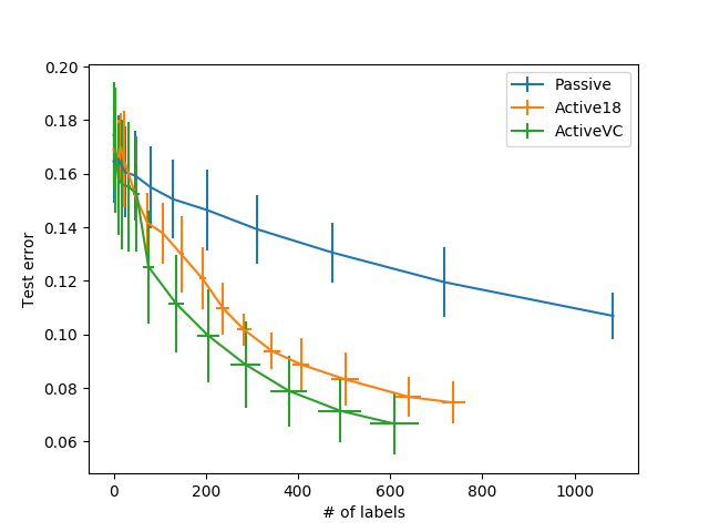
(a) Certainty

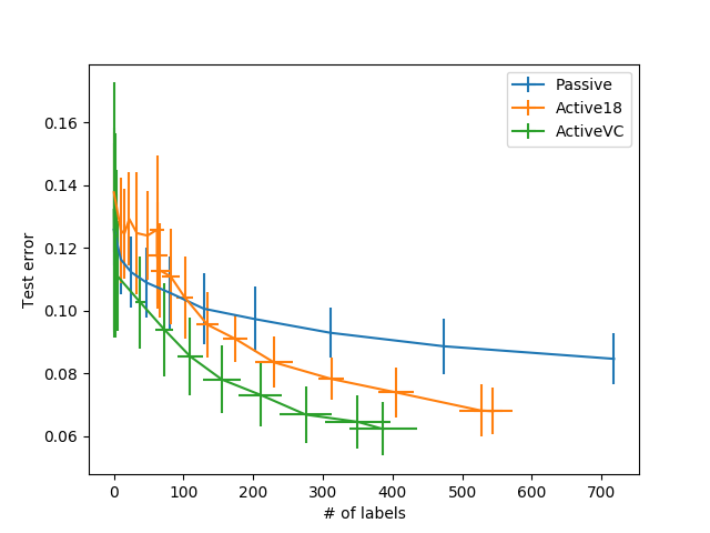
(b) Uncertainty

Figure 1: Test error vs the number of labels under different logging policies with the best parameters.

We plot test error as a function of the number of labels in Figure 1. It shows that test errors achieved by the proposed method drop faster than both the passive learning baseline, and the prior work [25] which does not apply variance control techniques. Additionally, as the number of labels grows, the gap widens.

References

- [1] Vowpal Wabbit. https://github.com/JohnLangford/vowpal_wabbit/.
- [2] Aman Agarwal, Soumya Basu, Tobias Schnabel, and Thorsten Joachims. Effective evaluation using logged bandit feedback from multiple loggers. arXiv preprint arXiv:1703.06180, 2017.
- [3] Onur Atan, William R. Zame, and Mihaela van der Schaar. Sequential patient recruitment and allocation for adaptive clinical trials. In Kamalika Chaudhuri and Masashi Sugiyama, editors, Proceedings of Machine Learning Research, volume 89 of Proceedings of Machine Learning Research, pages 1891–1900. PMLR, 16–18 Apr 2019.
- [4] M.-F. Balcan, A. Beygelzimer, and J. Langford. Agnostic active learning. J. Comput. Syst. Sci., 75(1):78–89, 2009.
- [5] P Borjesson and C-E Sundberg. Simple approximations of the error function q (x) for communications applications. IEEE Transactions on Communications, 27(3):639–643, 1979.
- [6] Léon Bottou, Jonas Peters, Joaquin Quiñonero-Candela, Denis X Charles, D Max Chickering, Elon Portugaly, Dipankar Ray, Patrice Simard, and Ed Snelson. Counterfactual reasoning and learning systems: The example of computational advertising. The Journal of Machine Learning Research, 14(1):3207–3260, 2013.
- [7] D. A. Cohn, L. E. Atlas, and R. E. Ladner. Improving generalization with active learning. Machine Learning, 15(2), 1994.
- [8] Corinna Cortes, Yishay Mansour, and Mehryar Mohri. Learning bounds for importance weighting. In Advances in neural information processing systems, pages 442–450, 2010.
- [9] S. Dasgupta, D. Hsu, and C. Monteleoni. A general agnostic active learning algorithm. In NIPS, 2007.
- [10] S. Hanneke. A bound on the label complexity of agnostic active learning. In ICML, 2007.
- [11] Steve Hanneke et al. Theory of disagreement-based active learning. Foundations and Trends® in Machine Learning, 7(2-3):131–309, 2014.
- [12] D. Hsu. Algorithms for Active Learning. PhD thesis, UC San Diego, 2010.
- [13] Tzu-Kuo Huang, Alekh Agarwal, Daniel J Hsu, John Langford, and Robert E Schapire. Efficient and parsimonious agnostic active learning. In Advances in Neural Information Processing Systems, pages 2755–2763, 2015.
- [14] David Kale, Marjan Ghazvininejad, Anil Ramakrishna, Jingrui He, and Yan Liu. Hierarchical active transfer learning. In Proceedings of the 2015 SIAM International Conference on Data Mining, pages 514–522. SIAM, 2015.
- [15] Samory Kpotufe and Guillaume Martinet. Marginal singularity, and the benefits of labels in covariate-shift. In Conference On Learning Theory, pages 1882–1886, 2018.
- [16] Akshay Krishnamurthy, Alekh Agarwal, Tzu-Kuo Huang, Hal Daumé, III, and John Langford. Active learning for cost-sensitive classification. In Doina Precup and Yee Whye Teh, editors, Proceedings of the 34th International Conference on Machine Learning, volume 70 of Proceedings of Machine Learning Research, pages 1915–1924, International Convention Centre, Sydney, Australia, 06–11 Aug 2017. PMLR.
- [17] A Maurer and M Pontil. Empirical bernstein bounds and sample variance penalization. In COLT 2009-The 22nd Conference on Learning Theory, 2009.
- [18] Hongseok Namkoong and John C Duchi. Variance-based regularization with convex objectives. In Advances in Neural Information Processing Systems, pages 2971–2980, 2017.
- [19] Paul R Rosenbaum and Donald B Rubin. The central role of the propensity score in observational studies for causal effects. Biometrika, 70(1):41–55, 1983.
- [20] Avishek Saha, Piyush Rai, Hal Daumé, Suresh Venkatasubramanian, and Scott L DuVall. Active supervised domain adaptation. In Joint European Conference on Machine Learning and Knowledge Discovery in Databases, pages 97–112. Springer, 2011.
- [21] Iiris Sundin, Peter Schulam, Eero Siivola, Aki Vehtari, Suchi Saria, and Samuel Kaski. Active learning for decision-making from imbalanced observational data. arXiv preprint arXiv:1904.05268, 2019.
- [22] Adith Swaminathan and Thorsten Joachims. Counterfactual risk minimization: Learning from logged bandit feedback. In International Conference on Machine Learning, pages 814–823, 2015.
- [23] VN Vapnik and A Ya Chervonenkis. On the uniform convergence of relative frequencies of events to their probabilities. Theory of Probability and its Applications, 16(2):264, 1971.
- [24] Eric Veach and Leonidas J Guibas. Optimally combining sampling techniques for monte carlo rendering. In Proceedings of the 22nd annual conference on Computer graphics and interactive techniques, pages 419–428. ACM, 1995.
- [25] Songbai Yan, Kamalika Chaudhuri, and Tara Javidi. Active learning with logged data. In International Conference on Machine Learning, pages 5517–5526, 2018.
- [26] Chicheng Zhang, Alekh Agarwal, Hal Daumé III, John Langford, and Sahand N Negahban. Warm-starting contextual bandits: Robustly combining supervised and bandit feedback. arXiv preprint arXiv:1901.00301, 2019.
- [27] Zihan Zhang, Xiaoming Jin, Lianghao Li, Guiguang Ding, and Qiang Yang. Multi-domain active learning for recommendation. In Thirtieth AAAI Conference on Artificial Intelligence, 2016.
- [28] Andre M Zubkov and Aleksandr A Serov. A complete proof of universal inequalities for the distribution function of the binomial law. Theory of Probability & Its Applications, 57(3):539–544, 2013.